Method to Remove Tilt-to-Length Coupling Caused by Interference of Flat-Top Beam and Gaussian Beam

Abstract

We discuss the tilt-to-length (TTL) coupling noise caused by interference between a flat-top beam and a Gaussian beam. Several physical models are presented to research the effects of non-diffracted and diffracted beams on TTL noise. A special case that can remove TTL coupling noise is discovered and is verified via both theoretical analysis and numerical simulations. The proposed case could provide desirable suggestions for the construction of high-precision interferometers such as the Laser Interferometer Space Antenna (LISA), Taiji program, or other interferometry systems.

1. Introduction

In the detection processes of space-borne and long-baseline laser interferometers such as the Laser Interferometer Space Antenna (LISA) [1] and Taiji program [2,3], the coupling between the beam jitter and the path length readout represents a significant noise source, this coupling is called tilt-to-length (TTL) coupling [4]. In their current designs, the interferometer arm length of the LISA is 2.5 million kilometers, and Taiji is 3 million kilometers, meaning that a fundamental-mode Gaussian beam would travel millions of kilometers in space and expand into a huge fundamental-mode Gaussian wavefront. (The above is a simplified assumption; interested readers can find more detailed discussion in [5,6], but these discussions are beyond the scope of this paper). The wavefront would then be clipped into a flat-top beam and imaged via the local telescope to the local optical bench to interfere with the local Gaussian beam. The wavefront will suffer diffraction and its propagation direction will jitter because of beam clipping and pointing accuracy limitations, and when the obvious beam type differences between the two interfering beams are considered, the above factors will produce more complex noise in the length readout.

In this paper, both non-diffracted and diffracted models are constructed to research the interference between a flat-top beam and a Gaussian beam. Then a special case, in which the TTL noise can be made negligible by placing the beam waist in an appropriate position and using a suitably large detector without clipping, is found and is verified via both analytical solutions and numerical simulations.

2. Optical Model

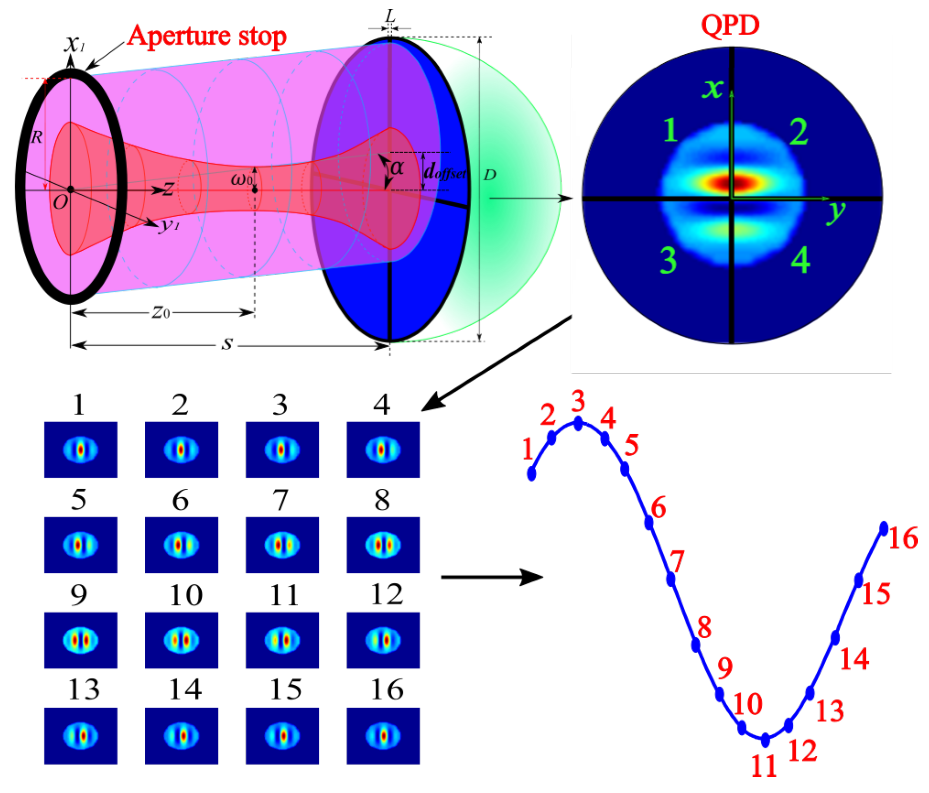
A simplified schematic of an interferometer is shown in the upper part of Figure 1; this interferometer includes a flat-top beam, a Gaussian beam, an aperture stop and a quadrant photo-diode (QPD). In the face of aperture, the flat-top beam can be regarded as a fraction of a plane wave. The electric field of an infinite plane wave can be given by:

$$E_{plane}=Aexp[-i(\overrightarrow{k}·\overrightarrow{r}-{\omega }_{1}t)]$$

(1)

Please note that A is the amplitude and is irrelevant to the pathlength signal, so it is set to unity here; ${\omega }_1$ is the angular frequency; $\overrightarrow{k}$ is the wave vector and its direction is ordinarily the direction in which the plane wave is traveling, so $|\overrightarrow{k}|=k=2\pi /\lambda$, where k is the wavenumber. $\overrightarrow{r}$ is the position vector that defines a point in three-dimensional space. Figure 1 shows that the direction cosine of $\overrightarrow{k}$ is $(sin\alpha ,0,cos\alpha )$. The non-diffractive form of the flat-top beam can be derived simply. In this situation, R can be regarded as the radial dimension of the flat-top beam, and a suitable expression for the flat-top beam is derived as shown in Equation (2). It is then very simple to calculate the complex amplitude of the flat-top beam on the detector by replacing “z” with “s” in Equation (2), s is the position of the detector.

$$E{(x,y,z)}_{flat}=\left\{\begin{array}{cc}exp[-ik(xsin\alpha +zcos\alpha )+i{\omega }_{1}t]\hfill & x^2+y^2\le R\hfill \\ 0\hfill & \mathrm{else}\hfill \end{array}\right.$$

(2)

The fundamental Gaussian beam serves as the most appropriate description for the output of most lasers. The amplitude of the electric field is also set to unity here and Gouy phase is assumed to be static phase and can thus be ignored in the situation shown in Figure 1, the electric field can then be written as:

$$E{(x,y,z)}_{gauss}=exp[-ik(\frac{x^2+y^2}{2q}+z-z_0)+i{\omega }_{2}t]$$

(3)

where the complex parameter $q=(z-z_0)+i{z}_r$, the Rayleigh range $z_r=\pi {\omega }_0^2/\lambda$, ${\omega }_0$ is the waist radius, $z_0$ is the z-axis value of the waist position, and ${\omega }_2$ is the frequency.

Next, we analyze the diffraction form. When a beam travels through free space, Kirchhoff’s diffraction formula can be used to calculate the beam model of diffracted propagation. As shown in Figure 1, the coordinates on the aperture are represented by $x_1$,$y_1$, while the coordinates on the detector are represented by x,y. Therefore, the field distribution $E{(x,y)}_{diff}$ of the diffracted beam on the detector can be calculated as:

$$E{(x,y)}_{diff}=\frac{1}{i\lambda }{\int }_{-\infty }^{\infty }{\int }_{-\infty }^{\infty }\frac{exp\left(ikr\right)}{r}\frac{1+cos\theta }{2}{E}_{aper}(x_1,y_1)d{x}_{1}d{y}_1$$

$$r=\sqrt{z^2+{(x-x_1)}^2+{(y-y_1)}^2},cos\theta =\frac{z}{r}$$

(4)

where r is the distance between point $(x,y)$ and point $(x_1,y_1)$, and $E_{aper}(x_1,y_1)$ is the pre-diffracted complex amplitude of beam on the aperture.

In current high-precision laser interferometers such as LISA or Taiji, heterodyne interference is used as the method of measurement, the QPD is usually used as the detector. And phasemeter is then used to analyze the photocurrents generated on the QPD to obtain the pathlength signal [7]. The optical simulation software ”ASAP”, known throughout the optics industry for its accuracy and efficiency on optical modelling, is used as the modelling tool to simulate heterodyne interference and obtain beat signal on detector. Then MATLAB is used as signal-processing tool to imitate the quadrature-phase(IQ) demodulation technique, which is used on the phasemeter of LISA pathfinder to compute interference signals [7]. An example is shown in the lower part of Figure 1, where the sampling number of the beat period is 16. The following simulations in Section 3.1 adopted the above way to perform the numerical analyses.

3. Theoretical Analysis

In the current theoretical analysis, the complex amplitude is normally used to calculate the phase information [8,9]:

$$C={\int }_S{E}_{meas}{E}_{ref}^{*}d{r}^2$$

(5)

Because the QPD has four segments as shown in Figure 1, it gives researchers some degrees of freedom to define signals with different pathlengths. The phase definition selected by LISA Pathfinder is LISA Pathfinder (LPF) signal, which first sums the complex amplitudes of each quadrant of QPD and then uses the following argument [10]:

$${\varphi }_{LPF}=arg\left(\sum _{n=1}^4{C}_n\right)$$

(6)

We focus here on the change in the optical path difference between the two beams. Because the path difference does not change over time, we can set t = 0 in the theoretical analysis. In addition, to simplify the calculations and obtain intuitive analytical solutions that clearly illustrate the parameter interdependency, we remove some of the terms that are unrelated to $\alpha$ from the calculation.

3.1. Non-Diffractive Form

The aperture stop in Figure 1 is moved to the front of the detector along the z-axis, but the rotation point of the flat-top beam is fixed and its size is assumed to be larger than the aperture stop in this analysis. So, beams can propagate freely without being diffracted. Then we derive the analytical expressions for the complex amplitude of each quadrant on the detector without diffraction. To research how the different factors are coupled into the measured path length, the final computation results will be visually decomposed into the sum of the different corresponding formulas in the simplification process. In Figure 1, the flat-top beam is rotated along the y-axis, so quadrants 1, and 2 have the same field distribution, and quadrants 3, and 4 have the same field distribution:

$$\begin{array}{cc}\hfill C_1=C_2& =\frac{1}{2}{\int }_{-R}^R\left({\int }_{L/2}^R{E}_{flat}{E}_{gauss}^{*}dx\right)dy\hfill \\ \hfill & \stackrel{}{\approx }\frac{1}{2}ϵexp\left(-\frac{1}{2}ikz{sin}^2\left(\alpha \right)+ikz(1-cos\left(\alpha \right))+\frac{1}{2}ik{z}_0{sin}^2\left(\alpha \right)\right)(F(L/2)+F\left(R\right))\hfill \end{array}$$

(7)

$$\begin{array}{cc}\hfill C_3=C_4& =\frac{1}{2}{\int }_{-R}^R\left({\int }_{-R}^{-L/2}{E}_{flat}{E}_{gauss}^{*}dx\right)dy\hfill \\ \hfill & \stackrel{}{\approx }\frac{1}{2}ϵexp\left(-\frac{1}{2}ikz{sin}^2\left(\alpha \right)+ikz(1-cos\left(\alpha \right))+\frac{1}{2}ik{z}_0{sin}^2\left(\alpha \right)\right)(F(-L/2)+F(-R))\hfill \end{array}$$

(8)

with:

$$F\left(r\right)=\mathrm{Erfi}\left[\frac{\left(\frac{1}{2}+\frac{i}{2}\right)\sqrt{k}(r-qsin\left(\alpha \right))}{\sqrt{q}}\right]$$

(9)

where $ϵ$ represents the collection of terms that are unrelated to $\alpha$, and will be ignored in the following calculation. The longitudinal pathlength signal (LPS) that results from LPF signal can then be derived as:

$$\begin{array}{ll}LP{S}_{LPF}& =\frac{arg\left({\sum }_{n=1}^4{C}_n\right)}{k}\\ & \stackrel{}{\approx }-\frac{1}{2}s{\alpha }^2+\frac{1}{2}(s-z_0){\alpha }^2\\ & +\frac{arg\left[2\left(F(L/2)+F\left(R\right)\right)+2\left(F(-L/2)+F\left(-R\right)\right)\right]}{k}\end{array}$$

(10)

We then set $L=0$ and $D/2=R=\infty$ to give the idealized detector shape and integral area. Formulas are presented using Taylor expansions based on the premise of preserving the precision of the calculations to obtain more intuitive analytical expressions. The $LP{S}_{LPF}$ is then changed to:

$$\begin{array}{c}\hfill LP{S}_{LPF}\stackrel{}{\approx }-\frac{1}{2}s{\alpha }^2+\frac{1}{2}(s-z_0){\alpha }^2+O\left({\alpha }^4\right)\end{array}$$

(11)

In the case shown in Figure 1, the geometrical optical path difference ($LP{S}_{OPD}$) between the two beams can be derived easily as:

$$LP{S}_{OPD}=\left(\frac{1}{cos\alpha }-1\right)·s\approx -\frac{1}{2}s{\alpha }^2+O\left({\alpha }^4\right)$$

(12)

The above obviously shows that when compared with $LP{S}_{OPD}$, $LP{S}_{LPF}$ contains extra terms, including the factor “$s-z_0$”. Figure 1 shows that “$s-z_0$” is the distance between the waist position and the detector, which determines the wavefront curvature of the Gaussian beam on the detector. When we set the beam waist on the detector, e.g., $z_0=s$, the wavefronts of the two beams on the detector are both planar. The pathlength signal is then caused by the geometric path only and not by the wavefront mismatch; therefore, $LP{S}_{LPF}$ is equal to $LP{S}_{OPD}$. Furthermore, Equation (11) illustrates an interesting phenomenon in that when the waist position of the Gaussian beam coincides with the pivot point of the flat-top beam, e.g., when $z_0=0$, the pathlength generated by the wavefront mismatch then has the same magnitude as $LP{S}_{OPD}$ but a different sign. The resulting $LP{S}_{LPF}$ then becomes negligible. However, Equation (10) indicates that the extra TTL coupling will be generated if the detector size is not large enough or its gap size is not equal to 0.

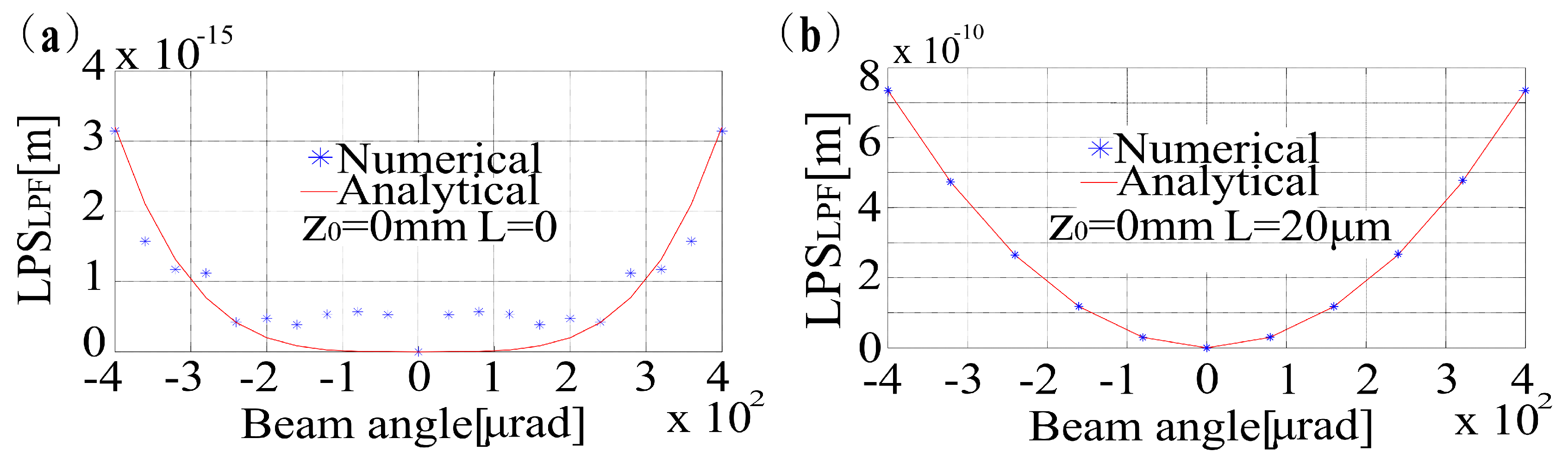
Next we use the numerical simulation tool to verify and increase confidence in the accuracy of the theoretical analysis above. In the simulation, we set the position of detector $s=500$ mm, the Gaussian waist ${\omega }_0=0.5$ mm and its waist position $z_0=0$. The radius dimension of flat-top beam $R=9$ mm, the diameter of detector $D=10$ mm, while the gap size of detector L is set to be 0 and 20 $\mathsf{\mu }$m respectively to enable observation of the change in $LP{S}_{LPF}$ with respect to the angle $\alpha$. The results are illustrated in Figure 2, which shows that the simulation results are in good agreement with the results derived from the analytical solution. Therefore, the TTL coupling in an interferometer with one Gaussian beam and one large flat-top beam and a large single-element photo-diode (SEPD) (i.e., a QPD with gap size equal to 0) can be made to vanish by setting appropriate optical parameters.

3.2. Diffraction

The basis of the situation shown in Figure 2a is that no diffraction occurs during the beam propagation process. However, the amplitude and the phase of flat-top beam wave on the detector could not be flat if diffraction occurred during propagation, but diffraction is very common in practical situations. Therefore, it is necessary to research whether the TTL coupling can also be eliminated as shown in Figure 2a when diffraction occurs.

The aperture stop is located on the coordinate origin O as shown in Figure 1 in this case. For consistency with Figure 2a, we also set s = 500 mm, ${\omega }_0$ = 0.5 mm, L = 0, and $z_0$ = 0 in the analysis. The diffraction effects regime could be determined by using the Fresnel number as follows:

$$N_F=\frac{R^2}{s\lambda }$$

(13)

Fresnel numbers of around 1 or higher characterize a case of Fresnel diffraction (near-field diffraction). From Equation (13) we know that when $N_F$ is approximately 1, then R is approximately 0.7 mm. We thus set R = 0.7 mm to study the effect of the Fresnel diffraction and set D = 30 mm to ensure that almost all the energy is detected. Equation (4) is used to calculate the field distribution of the diffracted beam. The field distribution of the diffracted flat-top beam on detector in polar coordinates(i.e., $x_1={\rho }_{1}cos{\psi }_1,y_1={\rho }_{1}sin{\psi }_1,x=\rho cos\psi ,y=\rho sin\psi$) can then be written as:

$$E{(\rho ,\psi )}_{flat-diff}=\frac{1}{i\lambda }{\int }_0^{2\pi }{\int }_0^R\frac{exp\left(ikr\right)}{r}\frac{1+cos\theta }{2}exp[-ik({\rho }_{1}cos{\psi }_{1}sin\alpha )]{\rho }_{1}d{\rho }_{1}d{\psi }_1$$

(14)

The field distribution of the diffracted Gaussian beam on detector can then be written as

$$E{(\rho ,\psi )}_{Gauss-diff}=\frac{1}{i\lambda }{\int }_0^{2\pi }{\int }_0^R\frac{exp\left(ikr\right)}{r}\frac{1+cos\theta }{2}exp[-ik(\frac{{\rho }_1^2}{2(i{z}_r-z_0)}-z_0)]{\rho }_{1}d{\rho }_{1}d{\psi }_1$$

(15)

where $r=\sqrt{s^2+{(\rho cos\psi -{\rho }_{1}cos{\psi }_1)}^2+{(\rho sin\psi -{\rho }_{1}sin{\psi }_1)}^2}$, $cos\theta =\frac{s}{r}$. There we analyze two situations. The first is the case where the aperture stop only works for the flat-top beam and not for the Gaussian beam (sometimes no stop is present in the transmission path of the Gaussian beam). This leads to the path length change:

$$LP{S}_{LPF}=\frac{arg\left({\int }_0^{2\pi }{\int }_0^{D/2}{E}_{flat-diff}{E}_{gauss}^{*}\rho d\rho d\psi \right)}{k}$$

(16)

The second case is where both interfering beams are affected by the aperture diffraction. This leads to the path length change:

$$LP{S}_{LPF}=\frac{arg\left({\int }_0^{2\pi }{\int }_0^{D/2}{E}_{flat-diff}{E}_{gauss-diff}^{*}\rho d\rho d\psi \right)}{k}$$

(17)

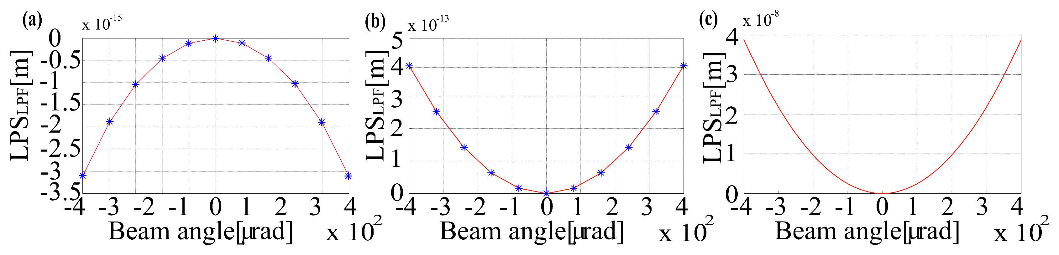
It is difficult to obtain analytic solutions for Equations (16) and (17), so numerical integrals are used to perform the analysis by using MATLAB (ASAP software was not selected due to data accuracy). The results for the two cases are shown in Figure 3a,b, respectively. Simultaneously, the analytical solution Equation (10) from the previous section is used to calculate the result for the case without diffraction for the comparison(the aperture stop is located on the detector). The result is shown in Figure 3c

Comparison of Figure 3a–c shows that in the case of interference between the non-diffracted flat-top beam and the Gaussian beam, the value of $LP{S}_{LPF}$ is close to that of $LP{S}_{OPD}$. The reason for this is that the small size of the flat-top beam reduces the degree of wavefront mismatch between the two beams and the geometric noise then becomes the main component of the TTL noise. However, when the two beams in the model or only flat-top beam used in the model are diffracted, the value of $LP{S}_{LPF}$ can be below the picometer order. This is similar to the situation shown in Figure 2a.

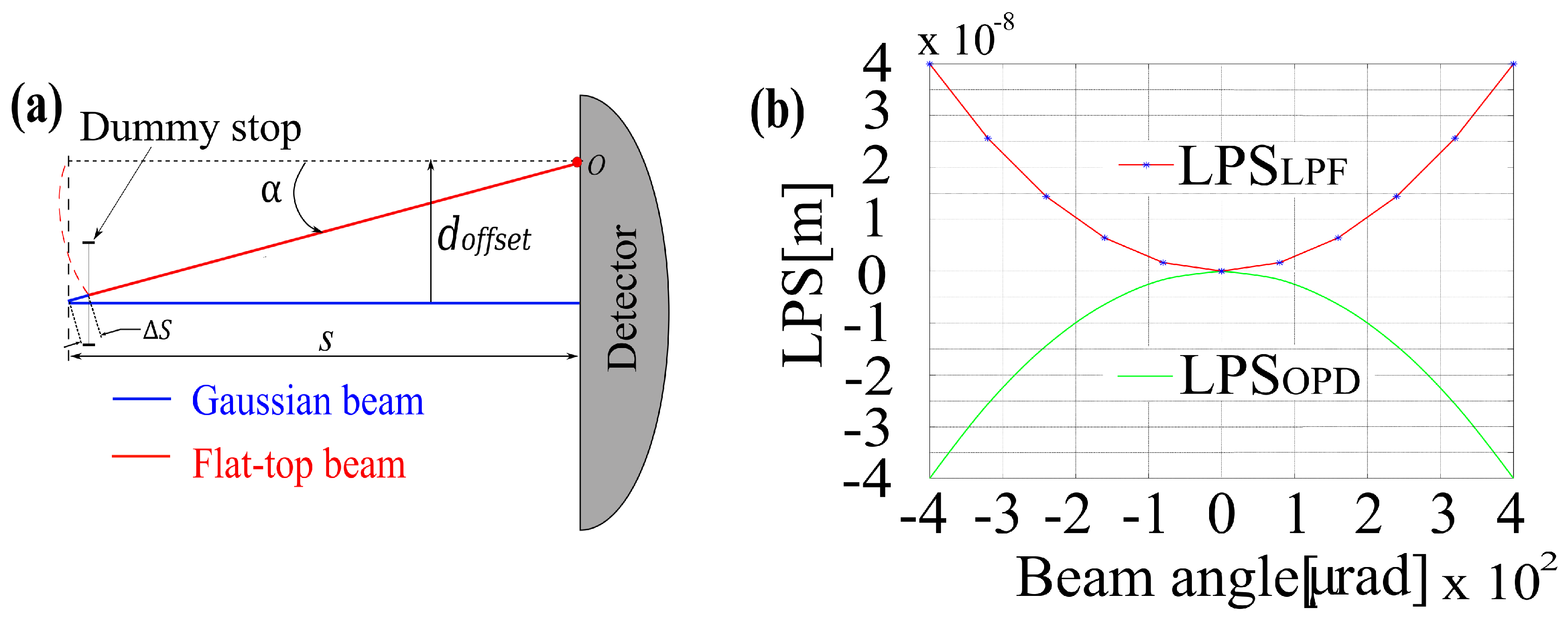
To explain why the TTL noise is eliminated in Figure 3a,b, the propagation path of flat-top beams is reset as shown and described in Figure 4a. The dynamic relationship between $\alpha$ and $d_{offset}$ is given by:

$$d_{offset}=stan\alpha$$

(18)

Then the propagation paths of the flat-top beams in Figure 4a and Figure 1 are the same and there is only a difference $\Delta S$ between them. We denote the coordinate system by ${\overrightarrow{r}}_{ref}$, the location of the pivot by ${\overrightarrow{p}}_{pivot}$, the translation vector by ${\overrightarrow{M}}_{trans}$, the rotation matrix for a rotation around the y-axis is $M_{rot}$

$$\begin{array}{c}\hfill {\overrightarrow{r}}_{ref}={(x_1,y_1,z)}^T,{\overrightarrow{p}}_{pivot}=(d_{offset},0,s)\\ \hfill {\overrightarrow{M}}_{trans}={(d_{offset},0,0)}^T,M_{rot}=\left(\begin{array}{ccc}cos\alpha & 0& -sin\alpha \\ 0& 1& 0\\ sin\alpha & 0& cos\alpha \end{array}\right)\end{array}$$

(19)

Then the transformed coordinate system ${\overrightarrow{r}}_{meas}$ is given by:

$${\overrightarrow{r}}_{meas}=M_{rot}^{-}({\overrightarrow{r}}_{ref}+M_{trans}-{\overrightarrow{p}}_{pivot})+{\overrightarrow{p}}_{pivot}=\left(\begin{array}{c}{x}_{1}cos\alpha +(z-s)sin\alpha +d_{offset}\\ y_1\\ (z-s)cos\alpha -xsin\alpha +s\end{array}\right)$$

(20)

Combining Equations (14), (18) and (20), The field distribution of the diffracted flat-top beam on detector in Figure 4 can be given by:

$$E{(\rho ,\psi )}_{flat-diff}=\frac{1}{i\lambda }{\int }_0^{2\pi }{\int }_0^R\frac{exp\left(ikr\right)}{r}\frac{1+cos\theta }{2}exp[-ik(s-{\rho }_{1}cos{\psi }_{1}sin\alpha -scos\alpha )]{\rho }_{1}d{\rho }_{1}d{\psi }_1$$

(21)

where $r=\sqrt{s^2+{[\rho cos\psi -({\rho }_{1}cos{\psi }_{1}cos\alpha -ssin\alpha +stan\alpha )]}^2+{(\rho sin\psi -{\rho }_{1}sin{\psi }_1)}^2}$, $cos\theta =\frac{s}{r}$. Then Equations (16) and (17) are used for numerical integration. The range of $\alpha$ is set also to −400 $\mathsf{\mu }$rad–400 $\mathsf{\mu }$rad in the calculations.

The two calculations present the same result, so just one $LP{S}_{LPF}$ is shown in Figure 4b. Simultaneously Equation (12) is used for calculating the geometric optical path difference. The results shows that while there is no geometric optical path difference between the two interference beams, the pathlength signal, which caused by the initial offset and the relative angle, has same magnitude as $LP{S}_{OPD}$ and a different sign. Therefore the reasons of the negligible TTL noise shown in Figure 3a,b can be regarded as the offset of the geometric optical path difference and the pathlength signal caused by lateral offset with the tilt between the two beams.

3.3. Discussion

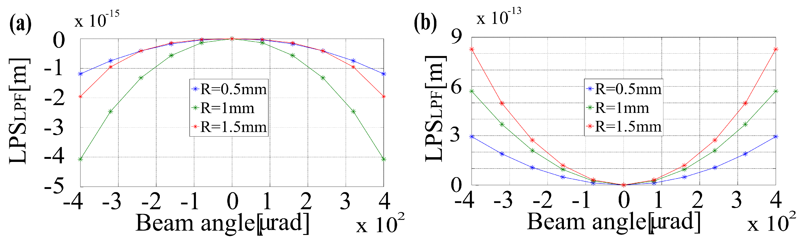
To increase the credibility of the conclusion, we respectively set the aperture stop size R = 0.5 mm, 1 mm, 1.5 mm to recalculate path length signals for the same situations in Figure 4a,b. The results are shown in Figure 5a,b. Therefore we can conclude that in the case of the diffraction model shown in Figure 1, the TTL coupling noise can be eliminated if the detector used is a large single-element photo-diode (SEPD) (i.e., a QPD with gap size equal to 0) and $z_0=0$ (even if the Gaussian beam is non-diffracted). This provides a different approach to use of an imaging system [11] which is based on Fermat’s principle of imaging the point of rotation onto the detector to eliminate the TTL noise.

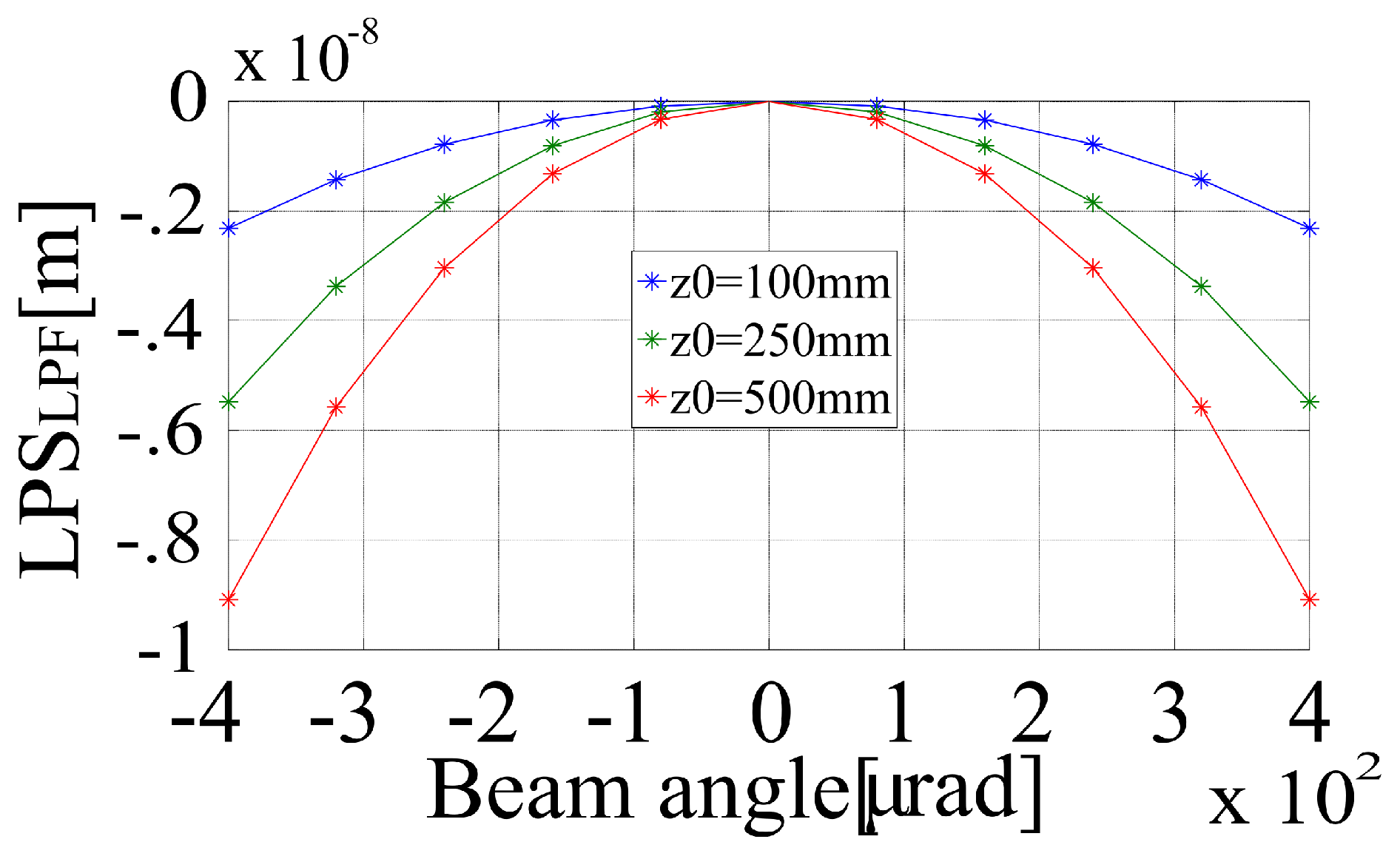
In reality, the balance that eliminates the TTL noise can be broken by other non-ideal factors, such as different beam parameters, beam misalignment, incomplete detection or wavefront aberrations. As an example, Figure 6 shows the numerical simulations of the coupling for the same situation in Figure 3a but with slightly different waist positions for the Gaussian beam.

4. Conclusions

Based on a non-diffracted model, we first derived the analytical form of the $LP{S}_{LPF}$ signal for interference between a flat-top beam and a Gaussian beam. We found that when the Gaussian beam waist position coincides with the rotation point of the flat-top beam, the TTL noise could be removed by using a large flat-top beam and an SEPD because of the offset between the geometric optical path and the pathlength caused by the wavefront mismatch. Similarly, for more general and practical diffraction models, the results show that the TTL noise can also be removed by the offset between the geometric optical path and the pathlength caused by a lateral offset with tilt. When the beam energy and the interference efficiency are considered, the above method may not be suitable for direct use in space optical systems for gravitational wave detection. However, the method can be adopted in ground interferometers or used in simulations to stabilize proposed systems or to study the effects of other factors on the optical path noise.

References

- Amaro-Seoane, P.; Audley, H.; Babak, S.; Baker, J.; Barausse, E.; Bender, P.; Berti, E.; Binetruy, P.; Born, M.; Bortoluzzi, D.; et al. Laser interferometer space antenna. arXiv 2017, arXiv:1702.00786. [Google Scholar]
- Zhi, W.; Wei, S.; Zhe, C. Preliminary design and analysis of telescope for space gravitational wave detection. Chin. Opt. 2018, 11, 131–151. [Google Scholar]
- Li, Y.; Liu, H.; Zhao, Y.; Sha, W.; Wang, Z.; Luo, Z.; Jin, G. Demonstration of an Ultraprecise Optical Bench for the Taiji Space Gravitational Wave Detection Pathfinder Mission. Appl. Sci. 2019, 9, 2087. [Google Scholar] [CrossRef]
- Schuster, S.; Wanner, G.; Tröbs, M.; Heinzel, G. Vanishing tilt-to-length coupling for a singular case in two-beam laser interferometers with Gaussian beams. Appl. Opt. 2015, 54, 1010–1014. [Google Scholar] [CrossRef] [PubMed] [Green Version]
- Bender, P.L. Wavefront distortion and beam pointing for LISA. Class. Quantum Gravity 2005, 22, S339–S346. [Google Scholar] [CrossRef]
- Waluschka, E. LISA Far-Field Phase Patterns. In Proceedings of the SPIE—The International Society for Optical Engineering, Denver, CO, USA, 23–27 June 1999; Volume 523. [Google Scholar]
- Gerberding, O.; Diekmann, C.; Kullmann, J.; Tröbs, M.; Bykov, I.; Barke, S.; Brause, N.C.; Esteban Delgado, J.J.; Schwarze, T.S.; Reiche, J. Readout for intersatellite laser interferometry: Measuring low frequency phase fluctuations of high-frequency signals with microradian precision. Rev. Sci. Instrum. 2015, 86, 074501. [Google Scholar] [CrossRef] [PubMed] [Green Version]
- Hechenblaikner, G. Measurement of the absolute wavefront curvature radius in a heterodyne interferometer. JOSA A 2010, 27, 2078–2083. [Google Scholar] [CrossRef] [PubMed]
- Girshovitz, P.; Shaked, N.T. Doubling the field of view in off-axis low-coherence interferometric imaging. Light Sci. Appl. 2014, 3, e151. [Google Scholar] [CrossRef]
- Wanner, G.; Schuster, S.; Tröbs, M.; Heinzel, G. A brief comparison of optical pathlength difference and various definitions for the interferometric phase. J. Phys. Conf. Ser. 2015, 610, 012043. [Google Scholar] [CrossRef]
- Schuster, S.; Tröbs, M.; Wanner, G.; Heinzel, G. Experimental demonstration of reduced tilt-to-length coupling by a two-lens imaging system. Opt. Express 2016, 24, 10466–10475. [Google Scholar] [CrossRef] [PubMed] [Green Version]
Figure 1.
The upper part of the figure is a simplified schematic of an interferometer. Here, we set a Gaussian beam as the reference beam that propagates along the z axis and strikes the center of the detector; We also set a flat-top beam as the measurement beam that is tilted by an angle around the y axis, and to simplify the calculations, we set its pivot as the coordinate origin O. The aperture stop is placed at the coordinate origin and is perpendicular to the z-axis and R is its radial dimension. s is the position of the QPD. is the distance between the centers of the two beams. is the waist position. D and L are the diameter size and the gap size of the QPD, respectively. The interference pattern per sampling on the detector shown as the left side of the lower part of the figure, is respectively summed over the area of detector to acquire a beat signal shown as the right side. The signal-processing tool based on MATLAB then can process the beat signal to obtain the phase information.
Figure 2.
(a) When the waist position of the Gaussian beam coincides with the rotation point of the flat-top beam and the detector is an large enough plane with no gap, is shown to be significantly below the picometer scale. (the differences are numerical errors related to the ray tracing algorithm). (b) When the gap size of detector is 20 m, the balance of (a) is disturbed and is shown to be increased to 10 pm order.
Figure 3.
Numerically computed results for interference of the diffracted flat-top beam with (a) a non-diffracted Gaussian beam and (b) a diffracted Gaussian beam. The analytically result obtained when both beams are non-diffracted is shown in (c).
Figure 4.
(a) The flat-top beam is placed with a transverse offset and a tilt angle around the pivot O on the detector. The dummy stop only works for flat-top beam and its center is always at the starting point of flat-top beam. There is no geometric path difference between the two beams in this case. (b) The upper part is the numerically computed results for interference between the flat-top beam and the Gaussian beam on the detector with an initial offset between the two beam centers. The lower part is analytically computed the geometric optical path difference .
Figure 5.
The TTL couplings shown in (a,b) are slightly different because of different optical parameters, but they are below the picometer order.
Figure 6.
When compared with Figure 3a, the result shows that the deviation of waist position of Gaussian beam can break the balance of the coupling, therefore is increased to nanometer scale.
© 2019 by the authors. Licensee MDPI, Basel, Switzerland. This article is an open access article distributed under the terms and conditions of the Creative Commons Attribution (CC BY) license (http://creativecommons.org/licenses/by/4.0/).
Share and Cite
MDPI and ACS Style
Zhao, Y.; Wang, Z.; Li, Y.; Fang, C.; Liu, H.; Gao, H. Method to Remove Tilt-to-Length Coupling Caused by Interference of Flat-Top Beam and Gaussian Beam. Appl. Sci. 2019, 9, 4112. https://0-doi-org.brum.beds.ac.uk/10.3390/app9194112
AMA Style
Zhao Y, Wang Z, Li Y, Fang C, Liu H, Gao H. Method to Remove Tilt-to-Length Coupling Caused by Interference of Flat-Top Beam and Gaussian Beam. Applied Sciences. 2019; 9(19):4112. https://0-doi-org.brum.beds.ac.uk/10.3390/app9194112
Chicago/Turabian StyleZhao, Ya, Zhi Wang, Yupeng Li, Chao Fang, Heshan Liu, and Huilong Gao. 2019. "Method to Remove Tilt-to-Length Coupling Caused by Interference of Flat-Top Beam and Gaussian Beam" Applied Sciences 9, no. 19: 4112. https://0-doi-org.brum.beds.ac.uk/10.3390/app9194112
Note that from the first issue of 2016, this journal uses article numbers instead of page numbers. See further details here.