Joint User Pairing, Channel Assignment and Power Allocation in NOMA based CR Systems

Abstract

The fifth generation (5G) wireless communication systems promise to provide massive connectivity over the limited available spectrum. Various new transmission paradigms such as non-orthogonal multiple access (NOMA) and cognitive radio (CR) have emerged as potential 5G enabling technologies. These techniques offer high spectral efficiency by allowing multiple users to communicate on the same frequency channel, simultaneously. A combination of both techniques may further enhance the performance of the system. This work aims to maximize the achievable rate of a multi-user multi-channel NOMA based CR system. We propose an efficient user pairing, channel assignment and power optimization technique for the secondary users while the performance of primary users is guaranteed through interference temperature limits. The results show that, at small values of the power budget or high interference threshold, optimizing channel allocation and user pairing proves to be more beneficial than optimal power allocation to the user pairs. The proposed joint optimization technique provides promising results for all values of the power budget, interference threshold and rate requirement of the communicating users.

1. Introduction

Orthogonal multiple access (OMA) techniques have proven their efficiency in the fourth generation (4G) of communication systems [1,2]. However, the high spectral efficiency requirements of the fifth generation (5G) of communication systems call for better technologies. Recently, non-orthogonal multiple access (NOMA) [3] has come forward and been shown to outperform OMA [4]. Some common techniques of NOMA include index modulation [5,6], code division [7], and power domain [8]. The power domain NOMA is considered to be the backbone of the 5G communication networks because of least computational complexity and excellent performance. Hence, this paper focuses on power domain type of NOMA. In NOMA, the signals of different users are transmitted simultaneously on the same channel with different power levels. Then, on reception successive interference cancellation (SIC) is employed to remove the interference where possible. In NOMA, each channel is shared by multiple users. Thus, the spectrum efficiency of NOMA systems is very high [9]. In multi user NOMA systems the complexity and delay because of SIC increases rapidly with the number of users sharing a channel. Hence, in a practical scenario, it becomes more beneficial to consider a combination of NOMA and OMA where the available spectrum is divided into multiple channels and each channel is shared by multiple users in a NOMA fashion. Similarly, the cognitive radio (CR) also offers high spectral efficiency. The CR employs the idea of spectrum reuse to offer high spectral efficiency. In CR, the licensed primary users (PUs) and unlicensed secondary users (SUs) communicate on the same channel, simultaneously. However, the SUs are required to keep the transmission power at a low level so that the PUs would not face harmful interference [10].

Optimization of resource allocation can significantly enhance the performance of a communication systems [11]. The problem of optimizing resource allocation in CR and NOMA systems have been considered multiple times in the literature. The authors of [12] optimized power allocation to minimize the energy consumption in a NOMA system. In [13], the authors allocated power in a NOMA system to guarantee the minimum quality of service (QoS) requirement of every user. The authors of [14] proposed a technique for energy efficiency maximization in NOMA systems. In [15], the authors studied power allocation in NOMA systems to maximize the secrecy rate of communicating users. The problem of maximizing sum rate in a NOMA system was considered by [16]. However, the work considered just two user NOMA case and did not guarantee the rate requirement of the users. Considering the problem of achieving fairness in NOMA systems, the authors of [17] proposed a sequential quadratic programming based solution. For CR systems, the authors of [18] optimized power loading for maximizing the energy efficiency of the communication system. In [19], the authors optimized power allocation to enhance the security of a CR system with a secondary receiver and one eves dropper. The authors of [12,13,14,15,16,17] considered single channel communication that cannot be directly mapped to multi channel systems. In NOMA, the delay of SIC increases with the number of users, hence, it is not feasible for all the users in the systems to communicate on a single channel. Thus, the solutions provided in [12,13,14,15,16,17] lack practical application. A CR system is expected to accommodate multiple SUs. However, in [18,19], the authors considered single SU. Some works in the literature [20,21] have also consider multi user CR systems however did not consider the optimization of power allocation.

Joint optimization of power and channel allocation can further enhance the performance of the systems. The authors of [22] optimized power and channel allocation in NOMA systems to minimize the power consumption of the network. [23] considered multi user NOMA system for energy efficiency maximization. The problem of sum rate maximization in in multi user NOMA systems was considered by [24]. On the other hand, considering CR systems, the authors of [25] optimized power loading and channel allocation for achieving fairness among the SUs. [26] considered optimization of resource allocation for energy efficiency maximization in CR systems. The problem of maximizing the sum rate in a CR system was solved in [27]. Integration of the NOMA into cognitive radio systems can result in further improvement in the network’s performance.

Some works in the literature have also considered resource allocation for NOMA based CR systems. The authors of [28] optimized power allocation to maximize the number of of admitted SUs in the system. [29] discussed sum rate maximization in a NOMA based CR system. The works reported in the literature have many deficiencies. The NOMA problems considered in [12,14,15,16,22,24,28] ignored the required minimum gap in received power for SIC. Similarly, the frameworks proposed in [16,18,19,24,27] did not consider the rate requirements of the communicating nodes. Some works [23,24,26,28] did not transform the problem to a convex form so the optimality of the solution cannot be guaranteed. Similar to the systems in [12,13,14,15,16,17,18,19], the NOMA based CR system considered in [29] consists of a single channel and the solution technique cannot be mapped to a multi channel scenario. In this work, we aim to maximize the sum rate in a multi user NOMA based underlay CR system. The main contribution of this work are listed below:

• A problem is formulated to maximize sum rate of a multi user NOMA based underlay CR system.
• Unlike previous works, the resource allocation is optimized while accounting for the rate requirement of each user and NOMA constraint of sufficient gap in received power for SIC. Further, the constraints of power budget and interference temperature are also taken into consideration.
• The original non convex optimization problem is transformed into a convex form and the closed form expressions for optimal power allocation are derived.
• An efficient technique for the user pairing and channel allocation is proposed.
• Simulation results thoroughly discuss the performance of the proposed technique.

The remainder of the paper is organized as follows. The system model and problem formulation is presented in Section 2. Section 3 provides the proposed solution technique. The simulation results are discussed in Section 4. Finally, the work is concluded in Section 5.

2. System Model and Problem Formulation

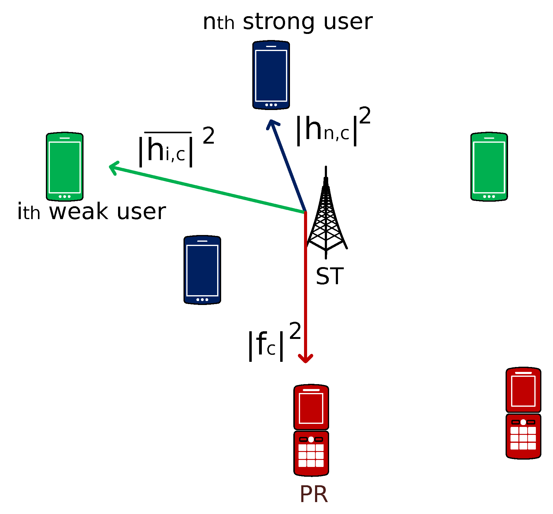
We consider a cooperative NOMA CR system where a secondary transmitter (ST) communicates with W number of secondary receivers (SRs) in the presence of primary receivers (PRs), as shown in Figure 1. The available spectrum is divided into $W/2$ channels and each channel is shared by two NOMA users. (The hardware complexity and delay due to SIC increase with the number of users per channel. Thus, the proposed system model considers two users per channel [30].) Without loss of generality, we consider the W users are sorted in descending order of their channel gains and divided into two sets of equal size. The set containing first ${\displaystyle \frac{W}{2}}$ users with larger values of channel gains is called the set of strong users and is represented as $\mathcal{A}$. Similarly, the users in the second set are called weak users because they have weak channel conditions compared to the nodes in the set of strong users; the set of weak user is denoted as $\mathcal{B}$. On each channel, a strong user is paired with a weak user. Then, on reception the strong user employs SIC to decode its signal without any interference from the weak user, whereas the weak user faces interference because of the strong users signal. The gains of the cth channel from ST to nth strong user and ith weak user are represented as $|h_{n,c}{|}^2$ and $|\overline{h_{i,c}}{|}^2$, respectively. The channel gain from ST to the PRs at the cth channel is denoted as $|f_c|$. To facilitate the mathematical formulation of the problem, a binary variable $x_{n,i,c}$ is introduced such that:

$$\begin{array}{c}\hfill x_{n,i,c}=\left\{\begin{array}{c}1,\mathrm{when}n\mathrm{th}\mathrm{strong}\mathrm{user}\mathrm{is}\mathrm{paired}\mathrm{with}i\mathrm{th}\mathrm{weak}\mathrm{user}\mathrm{and}\mathrm{are}\mathrm{allocated}c\mathrm{th}\mathrm{channel},\hfill \\ \forall n\in \mathcal{A},i\in \mathcal{B}\hfill \\ 0,\mathrm{otherwise},\hfill \end{array}\right.\end{array}$$

We aim to maximize the sum rate of the NOMA system subject to the interference temperature of the primary network, QoS guarantee of each user, limited battery power at the BS and sufficient gap in the received powers for SIC. The problem can be mathematically written as:

P1:

$$\begin{array}{cc}\hfill & \underset{x_{n,i,c},P_{n,i,c},S_{n,i,c}}{max}\sum _{n=1}^{W/2}\sum _{i=1}^{W/2}\sum _{c=1}^{W/2}{x}_{n,i,c}\left({log}_2\left(1+{\displaystyle \frac{P_{n,i,c}{|h_{n,c}|}^2}{{\sigma }^2}}\right)+{log}_2\left(1+{\displaystyle \frac{S_{n,i,c}{|\overline{h_{i,c}}|}^2}{P_{n,i,c}{|\overline{h_{i,c}}|}^2+{\sigma }^2}}\right)\right),\forall n\in \mathcal{A},i\in \mathcal{B},\hfill \\ \hfill & \mathrm{s}.\mathrm{t}.\hfill \end{array}$$

(1)

$$\begin{array}{cc}\hfill & \sum _{n=1}^{W/2}\sum _{i=1}^{W/2}{x}_{n,i,c}(S_{n,i,c}|h_{n,c}{|}^2-P_{n,i,c}|h_{n,c}{|}^2)\ge \psi ,\forall c,n\in \mathcal{A},i\in \mathcal{B},\hfill \end{array}$$

(2)

$$\begin{array}{cc}\hfill & \sum _{n=1}^{W/2}\sum _{i=1}^{W/2}{x}_{n,i,c}(P_{n,i,c}+S_{n,i,c}){|f_c|}^2\le I_{th},\forall c,n\in \mathcal{A},i\in \mathcal{B},\hfill \end{array}$$

(3)

$$\begin{array}{cc}\hfill & \sum _{n=1}^{W/2}\sum _{i=1}^{W/2}\sum _{c=1}^{W/2}{x}_{n,i,c}(P_{n,i,c}+S_{n,i,c})\le P_T,\forall n\in \mathcal{A},i\in \mathcal{B},\hfill \end{array}$$

(4)

$$\begin{array}{cc}\hfill & \sum _{i=1}^{W/2}\sum _{c=1}^{W/2}{x}_{n,i,c}{log}_2\left(1+{\displaystyle \frac{P_{n,i,c}{|h_{n,c}|}^2}{{\sigma }^2}}\right)\ge R_T,\forall n,n\in \mathcal{A},i\in \mathcal{B},\hfill \end{array}$$

(5)

$$\begin{array}{cc}\hfill & \sum _{n=1}^{W/2}\sum _{c=1}^{W/2}{x}_{n,i,c}{log}_2\left(1+{\displaystyle \frac{S_{n,i,c}{|\overline{h_{i,c}}|}^2}{P_{n,i,c}{|\overline{h_{i,c}}|}^2+{\sigma }^2}}\right)\ge R_T,\forall i,n\in \mathcal{A},i\in \mathcal{B},\hfill \end{array}$$

(6)

$$\begin{array}{cc}\hfill & \sum _{n=1}^{W/2}\sum _{c=1}^{W/2}{x}_{n,i,c}=1,\forall i,n\in \mathcal{A},i\in \mathcal{B},\hfill \end{array}$$

(7)

$$\begin{array}{cc}\hfill & \sum _{i=1}^{W/2}\sum _{c=1}^{W/2}{x}_{n,i,c}=1,\forall n,n\in \mathcal{A},i\in \mathcal{B},\hfill \end{array}$$

(8)

$$\begin{array}{cc}\hfill & \sum _{n=1}^{W/2}\sum _{i=1}^{W/2}{x}_{n,i,c}=1,\forall c,n\in \mathcal{A},i\in \mathcal{B}.\hfill \end{array}$$

(9)

The objective of the problem is given in Equation (1) where ${\sigma }^2$ denotes the variance of additive white Gaussian noise (AWGN), $P_{n,i,c}$ is the power allocated for the signal of nth strong user paired with ith weak user at cth channel and $S_{n,i,c}$ represents the power of the ith weak user paired with nth strong user at the cth channel. The first term in the objective represents the rate of the strong user and the second term is the rate of the weak user paired with the corresponding strong user. For SIC, a sufficient gap in the received powers of the signals of the strong user and weak user is required and is ensured by Equation (2). To protect the PRs from harmful interference, we have Equation (3) where $I_{th}$ represents the interference threshold. The constraint in Equation (4) guarantees that the power allocation at the ST follows the power budget where $P_T$ is the available power at the ST. The minimum rate requirement ($R_T$) of each user is ensured by Equations (5) and (6). The constraint in Equation (7) guarantees that each weak user pairs with one and only one strong user and is allocated one channel. It is also required that every strong user must pair with only one weak user and communication on a single channel, this demand is mathematically written as in Equation (8). Finally, Equation (9) makes sure that each channel accommodate only one user pair.

3. Proposed Solution

The problem in P1 is complex, non-convex and is very hard to solve for optimal solution because of high inter-dependency and inseparable $S_{n,i,c}$. To make the problem more tractable, we propose to allocated power in two steps. First, to distribute the available power in all user pairs and then distribute the power among the users in the pair. The power allocated to the user pair consisting of nth strong user and ith weak user at cth channel is denoted as $Q_{n,i,c}$. Then, the fractions of $Q_{n,i,c}$ allocated for the signal of strong user is denoted as ${\alpha }_{n,i,c}$, and $(1-{\alpha }_{n,i,c})$ represents the fraction allocated to the weak user. Thus, the transmit powers are given by $P_{n,i,c}={\alpha }_{n,i,c}{Q}_{n,i,c}$ and $S_{n,i,c}=(1-{\alpha }_{n,i,c})Q_{n,i,c}$. After this, the transformed problem is given as:

P2:

$$\begin{array}{cc}\hfill & \underset{x_{n,i,c},Q_{n,i,c},{\alpha }_{n,i,c}}{max}\sum _{n=1}^{W/2}\sum _{i=1}^{W/2}\sum _{c=1}^{W/2}{x}_{n,i,c}\left({log}_2\left(1+{\displaystyle \frac{{\alpha }_{n,i,c}{Q}_{n,i,c}{|h_{n,c}|}^2}{{\sigma }^2}}\right)+{log}_2\left(1+{\displaystyle \frac{(1-{\alpha }_{n,i,c})Q_{n,i,c}{|\overline{h_{i,c}}|}^2}{{\alpha }_{n,i,c}{Q}_{n,i,c}{|\overline{h_{i,c}}|}^2+{\sigma }^2}}\right)\right),\forall n\in \mathcal{A},i\in \mathcal{B},\hfill \\ \hfill & \mathrm{s}.\mathrm{t}.\hfill \end{array}$$

(10)

$$\begin{array}{cc}\hfill & \sum _{n=1}^{W/2}\sum _{i=1}^{W/2}{x}_{n,i,c}((1-{\alpha }_{n,i,c})Q_{n,i,c}|h_{n,c}{|}^2-{\alpha }_{n,i,c}{Q}_{n,i,c}|h_{n,c}{|}^2)\ge \psi ,\forall c,n\in \mathcal{A},i\in \mathcal{B},\hfill \end{array}$$

(11)

$$\begin{array}{cc}\hfill & \sum _{n=1}^{W/2}\sum _{i=1}^{W/2}{x}_{n,i,c}{Q}_{n,i,c}{|f_c|}^2\le I_{th}\forall c,n\in \mathcal{A},i\in \mathcal{B},\hfill \end{array}$$

(12)

$$\begin{array}{cc}\hfill & \sum _{n=1}^{W/2}\sum _{i=1}^{W/2}\sum _{c=1}^{W/2}{x}_{n,i,c}{Q}_{n,i,c}\le P_T,\forall n\in \mathcal{A},i\in \mathcal{B},\hfill \end{array}$$

(13)

$$\begin{array}{cc}\hfill & \sum _{i=1}^{W/2}\sum _{c=1}^{W/2}{x}_{n,i,c}{log}_2\left(1+{\displaystyle \frac{{\alpha }_{n,i,c}{Q}_{n,i,c}{|h_{n,c}|}^2}{{\sigma }^2}}\right)\ge R_T,\forall n,n\in \mathcal{A},i\in \mathcal{B},\hfill \end{array}$$

(14)

$$\begin{array}{cc}\hfill & \sum _{n=1}^{W/2}\sum _{c=1}^{W/2}{x}_{n,i,c}{log}_2\left(1+{\displaystyle \frac{(1-{\alpha }_{n,i,c})Q_{n,i,c}{|\overline{h_{i,c}}|}^2}{{\alpha }_{n,i,c}{Q}_{n,i,c}{|\overline{h_{i,c}}|}^2+{\sigma }^2}}\right)\ge R_T,\forall i,n\in \mathcal{A},i\in \mathcal{B},\hfill \end{array}$$

(15)

$$\begin{array}{cc}\hfill & 0\le {\alpha }_{n,i,c}\le 1,\forall c,n\in \mathcal{A},i\in \mathcal{B}.\hfill \end{array}$$

(16)

The problem in P2 is still non-convex because of Equations (10) and (15). To convert the problem in convex form, we substitute ${\beta }_{n,i,c}={\alpha }_{n,i,c}{Q}_{n,i,c}$, which makes the objective a convex function in ${\beta }_{n,i,c}$ and $Q_{n,i,c}$ (a discussion on the convexity of P2 and P3 is given in Appendix A). In addition, to transform the problem into a standard minimization problem, we multiply the objective by −1. The problem after transformation is:

P3:

$$\begin{array}{cc}\hfill & \underset{x_{n,i,c},Q_{n,i,c},{\beta }_{n,i,c}}{min}\sum _{n=1}^{W/2}\sum _{i=1}^{W/2}\sum _{c=1}^{W/2}-x_{n,i,c}\left({log}_2\left(1+{\displaystyle \frac{{\beta }_{n,i,c}{|h_{n,c}|}^2}{{\sigma }^2}}\right)+{log}_2\left(1+{\displaystyle \frac{(Q_{n,i,c}-{\beta }_{n,i,c}){|\overline{h_{i,c}}|}^2}{{\beta }_{n,i,c}{|\overline{h_{i,c}}|}^2+{\sigma }^2}}\right)\right),\forall n\in \mathcal{A},i\in \mathcal{B},\hfill \\ \hfill & \mathrm{s}.\mathrm{t}.\hfill \end{array}$$

(17)

$$\begin{array}{cc}\hfill & \sum _{n=1}^{W/2}\sum _{i=1}^{W/2}{x}_{n,i,c}((Q_{n,i,c}-{\beta }_{n,i,c})|h_{n,c}{|}^2-{\beta }_{n,i,c}|h_{n,c}{|}^2)\ge \psi ,\forall c,n\in \mathcal{A},i\in \mathcal{B},\hfill \end{array}$$

(18)

$$\begin{array}{cc}\hfill & \sum _{n=1}^{W/2}\sum _{i=1}^{W/2}{x}_{n,i,c}{Q}_{n,i,c}{|f_c|}^2\le I_{th}\forall c,n\in \mathcal{A},i\in \mathcal{B},\hfill \end{array}$$

(19)

$$\begin{array}{cc}\hfill & \sum _{n=1}^{W/2}\sum _{i=1}^{W/2}\sum _{c=1}^{W/2}{x}_{n,i,c}{Q}_{n,i,c}\le P_T,\forall n\in \mathcal{A},i\in \mathcal{B},\hfill \end{array}$$

(20)

$$\begin{array}{cc}\hfill & \sum _{i=1}^{W/2}\sum _{c=1}^{W/2}{x}_{n,i,c}{log}_2\left(1+{\displaystyle \frac{{\beta }_{n,i,c}{|h_{n,c}|}^2}{{\sigma }^2}}\right)\ge R_T,\forall n,n\in \mathcal{A},i\in \mathcal{B},\hfill \end{array}$$

(21)

$$\begin{array}{cc}\hfill & \sum _{n=1}^{W/2}\sum _{c=1}^{W/2}{x}_{n,i,c}{log}_2\left(1+{\displaystyle \frac{(Q_{n,i,c}-{\beta }_{n,i,c}){|\overline{h_{i,c}}|}^2}{{\beta }_{n,i,c}{|\overline{h_{i,c}}|}^2+{\sigma }^2}}\right)\ge R_T,\forall i,n\in \mathcal{A},i\in \mathcal{B},\hfill \end{array}$$

(22)

$$\begin{array}{cc}\hfill & {\beta }_{n,i,c}\ge 0,\forall n\in \mathcal{A},i\in \mathcal{B}.\hfill \end{array}$$

(23)

Although we have converted the objective of P3 to a convex form, the problem is still non-convex because of the constraint in Equation (22). We take advantage of the fact that Equation (22) is equivalent to:

$$\begin{array}{c}\hfill {log}_2\left(1+\sum _{n=1}^{W/2}\sum _{c=1}^{W/2}{x}_{n,i,c}\left({\displaystyle \frac{(Q_{n,i,c}-{\beta }_{n,i,c}){|\overline{h_{i,c}}|}^2}{{\beta }_{n,i,c}{|\overline{h_{i,c}}|}^2+{\sigma }^2}}\right)\right)\ge R_T,\forall i,n\in \mathcal{A},i\in \mathcal{B},\end{array}$$

(24)

then we can transform Equation (24) into a linear function as:

$$\begin{array}{cc}\hfill & \sum _{n=1}^{W/2}\sum _{c=1}^{W/2}{x}_{n,i,c}((Q_{n,i,c}-{\beta }_{n,i,c})|\overline{h_{i,c}}{|}^2-(2^{R_T}-1){\beta }_{n,i,c}|\overline{h_{i,c}}{|}^2)\ge (2^{R_T}-1){\sigma }^2,\forall i,n\in \mathcal{A},i\in \mathcal{B},\hfill \end{array}$$

(25)

Note that, if this technique were applied for transformation of Equation (15), it would result in a non-convex function because ${\alpha }_{n,i,c}{Q}_{n,i,c}$ makes the function non-convex. Similarly, we transform Equation (21) to a linear function to reduce the computational complexity. After the conversion, the constraint in Equation (21) is given by:

$$\begin{array}{cc}\hfill & \sum _{i=1}^{W/2}\sum _{c=1}^{W/2}{x}_{n,i,c}{\beta }_{n,i,c}{|h_{n,c}|}^2\ge (2^{R_T}-1){\sigma }^2,\forall n,n\in \mathcal{A},i\in \mathcal{B},\hfill \end{array}$$

(26)

For the given value of $x_{n,i,c}$, the problem is now convex. Hence, optimal solution can be obtained by employing duality theory [31]. The dual problem is given below:

$$\begin{array}{cc}\hfill & \underset{{\lambda }_i,{\mu }_c,\eta ,{\tau }_n,{\theta }_i}{max}D({\lambda }_i,{\mu }_c,\eta ,{\tau }_n,{\theta }_i),\hfill \\ \hfill & \mathrm{s}.\mathrm{t}.{\lambda }_i\ge 0,{\mu }_c\ge 0,\eta \ge 0,{\tau }_n\ge 0,{\theta }_i\ge 0,\forall n\in \mathcal{A},i\in \mathcal{B}.\hfill \end{array}$$

(27)

The $D({\lambda }_i,{\mu }_c,\eta ,{\tau }_n,{\theta }_i)$ in Equation (28) is called the dual function and ${\lambda }_i,{\mu }_c,\eta ,{\tau }_n,{\theta }_i$ are the dual variables. The dual function is given as:

$$\begin{array}{c}\hfill D({\lambda }_i,{\mu }_c,\eta ,{\tau }_n,{\theta }_i)=\underset{Q_{n,i,c},{\beta }_{n,i,c}}{min}L({\lambda }_i,{\mu }_c,\eta ,{\tau }_n,{\theta }_i,Q_{n,i,c},{\beta }_{n,i,c}),\forall n\in \mathcal{A},i\in \mathcal{B},\end{array}$$

(28)

where $L({\lambda }_i,{\mu }_c,\eta ,{\tau }_n,{\theta }_i,Q_{n,i,c},{\beta }_{n,i,c})$ is the Lagrangian of the problem and is written as:

$$\begin{array}{cc}\hfill L=& -\sum _{n=1}^{W/2}\sum _{i=1}^{W/2}\sum _{c=1}^{W/2}{x}_{n,i,c}{log}_2\left(1+{\displaystyle \frac{{\beta }_{n,i,c}{|h_{n,c}|}^2}{{\sigma }^2}}\right)+{log}_2\left(1+{\displaystyle \frac{(Q_{n,i,c}-{\beta }_{n,i,c}){|\overline{h_{i,c}}|}^2}{{\beta }_{n,i,c}{|\overline{h_{i,c}}|}^2+{\sigma }^2}}\right)+\sum _{c=1}^{W/2}{\lambda }_i\hfill \\ & (\psi -\sum _{n=1}^{W/2}\sum _{i=1}^{W/2}{x}_{n,i,c}(Q_{n,i,c}|h_{n,c}{|}^2-2{\beta }_{n,i,c}|h_{n,c}{|}^2\left)\right)+\sum _{c=1}^{W/2}{\mu }_c(\sum _{n=1}^{W/2}\sum _{i=1}^{W/2}{x}_{n,i,c}{Q}_{n,i,c}|f_c{|}^2-I_{th})+\hfill \\ & \eta (\sum _{n=1}^{W/2}\sum _{i=1}^{W/2}\sum _{c=1}^{W/2}{x}_{n,i,c}{Q}_{n,i,c}-P_T)+\sum _{n=1}^{W/2}{\tau }_n((2^{R_T}-1){\sigma }^2-(\sum _{i=1}^{W/2}\sum _{c=1}^{W/2}{x}_{n,i,c}{\beta }_{n,i,c}|h_{n,c}{|}^2\left)\right)+{\theta }_i\hfill \\ & \hfill ((2^{R_T}-1){\sigma }^2-(\sum _{n=1}^{W/2}\sum _{c=1}^{W/2}{x}_{n,i,c}((Q_{n,i,c}-{\beta }_{n,i,c})|\overline{h_{i,c}}{|}^2-(2^{R_T}-1){\beta }_{n,i,c}|\overline{h_{i,c}}{|}^2\left)\right)),\forall n\in \mathcal{A},i\in \mathcal{B}.\end{array}$$

(29)

Simplifying Equation (29), we get:

$$\begin{array}{cc}\hfill L=& \sum _{n=1}^{W/2}\sum _{i=1}^{W/2}\sum _{c=1}^{W/2}{x}_{n,i,c}(-{log}_2\left(1+{\displaystyle \frac{{\beta }_{n,i,c}{|h_{n,c}|}^2}{{\sigma }^2}}\right)-{log}_2\left(1+{\displaystyle \frac{(Q_{n,i,c}-{\beta }_{n,i,c}){|\overline{h_{i,c}}|}^2}{{\beta }_{n,i,c}{|\overline{h_{i,c}}|}^2+{\sigma }^2}}\right)-{\lambda }_i\hfill \\ & (Q_{n,i,c}|h_{n,c}{|}^2-2{\beta }_{n,i,c}|h_{n,c}{|}^2)+{\mu }_c(Q_{n,i,c}|f_c{|}^2)+\eta Q_{n,i,c}-{\tau }_n({\beta }_{n,i,c}|h_{n,c}{|}^2)-{\theta }_i\left(\right(Q_{n,i,c}-\hfill \\ & {\beta }_{n,i,c})|\overline{h_{i,c}}{|}^2-(2^{R_T}-1){\beta }_{n,i,c}|\overline{h_{i,c}}{|}^2))+\sum _{i=1}^{W/2}{\lambda }_i\psi -\sum _{c=1}^{W/2}{\mu }_c{I}_{th}-\eta P_T+\sum _{n=1}^{W/2}{\tau }_n(2^{R_T}-1){\sigma }^2\hfill \\ & +\sum _{i=1}^{W/2}{\theta }_i(2^{R_T}-1){\sigma }^2,\forall n\in \mathcal{A},i\in \mathcal{B}.\hfill \end{array}$$

(30)

Note that ${\sum }_{i=1}^{W/2}{\lambda }_i\psi -{\sum }_{c=1}^{W/2}{\mu }_c{I}_{th}-\eta P_T+{\sum }_{n=1}^{W/2}{\tau }_n(2^{R_T}-1){\sigma }^2+{\sum }_{i=1}^{W/2}{\theta }_i(2^{R_T}-1){\sigma }^2$ are constants, thus can be ignored. The problem can be decomposed into following ${\displaystyle \frac{W^3}{8}}$ sub-problems:

$$\begin{array}{c}\underset{{\beta }_{n,i,c},Q_{n,i,c}}{min}(-{log}_2\left(1+{\displaystyle \frac{{\beta }_{n,i,c}{|h_{n,c}|}^2}{{\sigma }^2}}\right)-{log}_2\left(1+{\displaystyle \frac{(Q_{n,i,c}-{\beta }_{n,i,c}){|\overline{h_{i,c}}|}^2}{{\beta }_{n,i,c}{|\overline{h_{i,c}}|}^2+{\sigma }^2}}\right)-{\lambda }_i\hfill \\ (Q_{n,i,c}|h_{n,c}{|}^2-2{\beta }_{n,i,c}|h_{n,c}{|}^2)+{\mu }_c(Q_{n,i,c}|f_c{|}^2)+\eta \left(Q_{n,i,c}\right)-{\tau }_n({\beta }_{n,i,c}|h_{n,c}{|}^2)-{\theta }_i\hfill \\ ((Q_{n,i,c}-{\beta }_{n,i,c})|\overline{h_{i,c}}{|}^2-(2^{R_T}-1){\beta }_{n,i,c}|\overline{h_{i,c}}{|}^2)),\forall n\in \mathcal{A},i\in \mathcal{B}.\hfill \end{array}$$

(31)

As the problem is convex, we can apply Karush–Kuhn–Tucker (KKT):

$$\begin{array}{l}-{\displaystyle \frac{|h_{n,c}{|}^2}{{\sigma }^2+{\beta }_{n,i,c}{|h_{n,c}|}^2}}-{\displaystyle \frac{{\displaystyle \frac{-({\sigma }^2+{\beta }_{n,i,c}|\overline{h_{i,c}}{|}^2)-(Q_{n,i,c}-{\beta }_{n,i,c}){|\overline{h_{i,c}}|}^4}{({\sigma }^2+{\beta }_{n,i,c}|\overline{h_{i,c}}{{|}^2)}^2}}}{{\displaystyle \frac{({\sigma }^2+{\beta }_{n,i,c}|\overline{h_{i,c}}{|}^2)+(Q_{n,i,c}-{\beta }_{n,i,c}){|\overline{h_{i,c}}|}^2}{{\sigma }^2+{\beta }_{n,i,c}{|h_{i,c}|}^2}}}}+2{\lambda }_i|h_{n,c}{|}^2-{\tau }_n|h_{n,c}{|}^2+{\theta }_i{|\overline{h_{i,c}}|}^2\hfill \\ +{\theta }_i(2^{R_T}-1){|\overline{h_{i,c}}|}^2=0.\hfill \end{array}$$

(32)

Simplifying Equation (32), we get:

$$\begin{array}{cc}\hfill & -{\displaystyle \frac{|h_{n,c}{|}^2}{{\sigma }^2+{\beta }_{n,i,c}{|h_{n,c}|}^2}}+{\displaystyle \frac{|\overline{h_{i,c}}{|}^2}{{\beta }_{n,i,c}{|\overline{h_{i,c}}|}^2+{\sigma }^2}}+2{\lambda }_i|h_{n,c}{|}^2-{\tau }_n|h_{n,c}{|}^2+{\theta }_i|\overline{h_{i,c}}{|}^2+{\theta }_i(2^{R_T}-1){|\overline{h_{i,c}}|}^2=0.\hfill \end{array}$$

(33)

Then, optimal value of ${\beta }_{n,i,c}$ is obtained as given below:

$$\begin{array}{c}\hfill {\beta }_{n,i,c}^{*}={\left({\displaystyle \frac{(-(|\overline{h_{i,c}}{|}^2+|h_{n,c}{|}^2){\sigma }^2(|h_{n,c}{|}^2(2{\lambda }_i-{\tau }_n)+2^{R_T}|\overline{h_{i,c}}{|}^2{\theta }_i)\pm \sqrt{{\mathsf{\Lambda }}_{n,i,c}}}{(2|\overline{h_{i,c}}{|}^2|h_{n,c}{|}^2(|h_{n,c}{|}^2(2{\lambda }_i-{\tau }_n)+2^{R_T}|\overline{h_{i,c}}{|}^2{\theta }_i\left)\right)}}\right)}^{+},\forall n\in \mathcal{A},i\in \mathcal{B},\end{array}$$

(34)

where ${\left(\varpi \right)}^{*}=max(\varpi ,0)$, and the value of ${\mathsf{\Lambda }}_{n,i,c}$ is given by:

$$\begin{array}{l}{\mathsf{\Lambda }}_{n,i,c}=\left(\right(-|\overline{h_{i,c}}{|}^2+|h_{n,c}{|}^2){\sigma }^2(|h_{n,c}{|}^2(2{\lambda }_i-{\tau }_n)+2^{R_T}|\overline{h_{i,c}}{|}^2{\theta }_i\left)\right(|h_{n,c}{|}^2(|h_{n,c}{|}^2{\sigma }^2(2{\lambda }_i-{\tau }_n)+\hfill \\ |\overline{h_{i,c}}{|}^2(4-2{\lambda }_i{\sigma }^2+{\sigma }^2{\tau }_n))+2^{R_T}|\overline{h_{i,c}}{|}^2(-|\overline{h_{i,c}}{|}^2+|h_{n,c}{|}^2){\sigma }^2{\theta }_i\left)\right)),\forall n\in \mathcal{A},i\in \mathcal{B},\hfill \end{array}$$

Similarly, the value of $Q_{n,i,c}$ is derived as:

$$\begin{array}{c}\hfill Q_{n,i,c}^{*}={\left(-{\displaystyle \frac{{\sigma }^2}{|\overline{h_{i,c}}{|}^2}}+{\displaystyle \frac{1}{-|h_{n,c}{|}^2{\lambda }_i+\eta -|\overline{h_{i,c}}{|}^2{\theta }_i+{|f_c|}^2{\mu }_c}}\right)}^{+},\forall n\in \mathcal{A},i\in \mathcal{B}.\end{array}$$

(35)

As now we have ${\beta }_{n,i,c}^{*}$ and $Q_{n,i,c}^{*}$, we can calculate ${\alpha }^{*}$ as:

$$\begin{array}{c}\hfill {\alpha }_{n,i,c}^{*}={\displaystyle \frac{{\beta }_{n,i,c}^{*}}{Q_{n,i,c}^{*}}},\forall n\in \mathcal{A},i\in \mathcal{B}.\end{array}$$

(36)

With this, the optimal values of $P_{n,i,c}$ and $S_{n,i,c}$ are given by:

$$\begin{array}{cc}\hfill & P_{n,i,c}^{*}={\alpha }_{n,i,c}^{*}{Q}_{n,i,c}^{*},\forall n\in \mathcal{A},i\in \mathcal{B}.\hfill \end{array}$$

(37)

$$\begin{array}{cc}\hfill & S_{n,i,c}^{*}=(1-{\alpha }_{n,i,c}^{*})Q_{n,i,c}^{*},\forall n\in \mathcal{A},i\in \mathcal{B}.\hfill \end{array}$$

(38)

Until this point, we have ignored $x_{n,i,c}$; now, the solution of following problem yields the solution of $x_{n,i,c}$:

$$\begin{array}{cc}\hfill & \underset{x_{n,i,c}}{min}\sum _{n=1}^{W/2}\sum _{i=1}^{W/2}\sum _{c=1}^{W/2}{\mathsf{\Psi }}_{n,i,c},\hfill \end{array}$$

(39)

where

$$\begin{array}{l}{\mathsf{\Psi }}_{n,i,c}=(-{log}_2\left(1+{\displaystyle \frac{{\beta }_{n,i,c}^{*}{|h_{n,c}|}^2}{{\sigma }^2}}\right)-{log}_2\left(1+{\displaystyle \frac{(Q_{n,i,c}^{*}-{\beta }_{n,i,c}^{*}){|\overline{h_{i,c}}|}^2}{{\beta }_{n,i,c}^{*}{|\overline{h_{i,c}}|}^2+{\sigma }^2}}\right)-{\lambda }_i(Q_{n,i,c}{|h_{n,c}|}^2\hfill \\ -2{\beta }_{n,i,c}^{*}|h_{n,c}{|}^2)+{\mu }_c(Q_{n,i,c}^{*}|f_c{|}^2)+\eta Q_{n,i,c}^{*}-{\tau }_n({\beta }_{n,i,c}^{*}|h_{n,c}{|}^2)-{\theta }_i((Q_{n,i,c}^{*}-{\beta }_{n,i,c}^{*}){|\overline{h_{i,c}}|}^2-\hfill \\ (2^{R_T}-1){\beta }_{n,i,c}^{*}|\overline{h_{i,c}}{|}^2)),\forall n\in \mathcal{A},i\in \mathcal{B}.\hfill \end{array}$$

To solve the problem, we propose the technique provided in Algorithm 1.

Algorithm 1 User pairing and channel allocation.

Initialize$x=zero\left({\displaystyle \frac{W}{2}},{\displaystyle \frac{W}{2}},{\displaystyle \frac{W}{2}}\right)$ Pair${\mathcal{A}}_n$ with ${\mathcal{B}}_{(W/2)+1-n},\forall n=1,2,3...{\displaystyle \frac{W}{2}}$, where ${\mathcal{A}}_n$ represents the nth user in the set of strong users sorted in descending order of channel gains and ${\mathcal{B}}_z$ denotes the zth user in the sorted set of all the weak users. Then, the nth user pair is given as ${\xi }_n$. Set$P_{{\mathcal{A}}_n}$ = $P_{{\mathcal{B}}_n}$ = ${\displaystyle \frac{P_T}{W}},\forall n=1,2,3,\dots {\displaystyle \frac{W}{2}}$. Calculate the rate of each user pair (${\xi }_n$) for every channel as ${\vartheta }_{{\xi }_n,c}={log}_2\left(1+{\displaystyle \frac{P_{{\mathcal{A}}_n}{|h_{{\mathcal{A}}_n,c}|}^2}{{\sigma }^2}}\right)+{log}_2\left(1+{\displaystyle \frac{P_{{\mathcal{B}}_{W+1-n}}{|h_{{\mathcal{B}}_{W+1-n},c}|}^2}{P_{{\mathcal{A}}_n}{|h_{{\mathcal{B}}_{W+1-n},c}|}^2+{\sigma }^2}}\right)$. Findl such that ${\vartheta }_{{\xi }_n,l}==max\left({\vartheta }_{{\xi }_n,c}\right)\forall c=1,2,3\dots {\displaystyle \frac{W}{2}}$. Set$x_{{\xi }_n,l}$ = 1. Remove user pair ${\xi }_n$ and channel l from the search. Repeat steps 2–7, ${\displaystyle \frac{W}{2}}-1$ times. Return$x_{n,i,c}^{*}$.

We know that a user with better channel conditions requires less power to achieve the required rate as compared to the user with bad channel conditions. Thus, if the very weak user is paired with a very strong user, the strong user would only require a little power to satisfy its rate, thus leaving large amount of available energy for the weak user. In this scheme, we pair the users such that the strongest user is paired with the weakest user. In Step 1, we initialize a three-dimensional matrix x having size ${\displaystyle \frac{W}{2}}$ in all dimensions. Then, in Step 2, we pair the users together such that the strongest user is paired with the weakest user, the second strongest user is paired with the second weakest and so on. In Step 3, to find the channel allocation, we first decide the available power equally among all the users. In Step 4, we calculate the rate of each user pair. Then, in Steps 5 and 6, we find the channels for which each respective pair provides maximum rate and assign that channel to the user pair, respectively. The user pair that has been allocated a channel is removed from the allocation process along with the allocated channel. As there are ${\displaystyle \frac{W}{2}}$ user pairs and channels, Steps 2–7 are repeated ${\displaystyle \frac{W}{2}}-1$ times because the last user pair is automatically assigned the last remaining channel.

Now, it remains to solve the dual problem. We employ sub-gradient method [32] to solve the problem for dual variables; the dual variable updates in the uth iteration are given by:

$$\begin{array}{cc}\hfill & {\lambda }_i^u={\lambda }_i^{u-1}+\delta \left(\psi -\sum _{n=1}^{W/2}\sum _{i=1}^{W/2}{x}_{n,i,c}(Q_{n,i,c}|h_{n,c}{|}^2-2{\beta }_{n,i,c}|h_{n,c}{|}^2)\right),\forall n\in \mathcal{A},i\in \mathcal{B},\hfill \\ \hfill & {\mu }_c^u={\mu }_c^{u-1}+\delta \left(\sum _{n=1}^{W/2}\sum _{i=1}^{W/2}{x}_{n,i,c}{Q}_{n,i,c}{|f_c|}^2-I_{th}\right),\forall n\in \mathcal{A},i\in \mathcal{B},\hfill \\ \hfill & {\eta }^u={\eta }^{u-1}+\delta \left(\sum _{n=1}^{W/2}\sum _{i=1}^{W/2}\sum _{c=1}^{W/2}{x}_{n,i,c}{Q}_{n,i,c}-P_T\right),\forall n\in \mathcal{A},i\in \mathcal{B},\hfill \\ \hfill & {\tau }_n^u={\tau }_n^{u-1}+\delta \left((2^{R_T}-1){\sigma }^2-\sum _{i=1}^{W/2}\sum _{c=1}^{W/2}{x}_{n,i,c}{\beta }_{n,i,c}{|h_{n,c}|}^2\right),\forall n\in \mathcal{A},i\in \mathcal{B},\hfill \\ \hfill & {\theta }_i^u={\theta }_i^{u-1}+\delta \left((2^{R_T}-1){\sigma }^2-\sum _{n=1}^{W/2}\sum _{c=1}^{W/2}{x}_{n,i,c}((Q_{n,i,c}-{\beta }_{n,i,c})|\overline{h_{i,c}}{|}^2-(2^{R_T}-1){\beta }_{n,i,c}|\overline{h_{i,c}}{|}^2)\right),\forall n\in \mathcal{A},i\in \mathcal{B},\hfill \end{array}$$

where $\delta$ is the step size.

4. Simulation Results

In this section, we demonstrate the performance of the proposed scheme. The comparison of the following techniques is presented:

• Opt: This refers to the joint power, user pairing and channel allocation technique presented in Section 3.
• Fix-${\mathbf{Q}}_{\mathbf{n},\mathbf{i},\mathbf{c}}$: In this case, we allocate equal amount of power to each user pair while keeping in account the interference constraint. Then, we optimize ${\alpha }_{n,i,c}$ and ${\mathbf{x}}_{\mathbf{n},\mathbf{i},\mathbf{c}}$ as proposed in Section 3. The power allocation to the pairs in this case is given by:

  $$\begin{array}{c}\hfill Q_{n,i,c}=min\left({\displaystyle \frac{P_T}{W/2}},{\displaystyle \frac{I_{th}}{|f_c{|}^2}}\right),\forall c,\forall n\in \mathcal{A},i\in \mathcal{B}.\end{array}$$
• Random-${\mathbf{x}}_{\mathbf{n},\mathbf{i},\mathbf{c}}$: In this technique, a user from the set of strong users is paired with a weak user at random, and then this pair is allocated a channel randomly. While the pairing and allocation is random, we keep in account that a strong user must only pair with one weak user and vice versa. Similarly, each channel is allocated to just one user pair and, further, a user pair cannot be assigned more than one channel.

For the simulations, we considered Rayleigh fading channels and the values of $W,{\sigma }^2,P_T,\psi ,R_T,\mathrm{and}{I}_{th}$ were taken to be 10, 0.01, 10 W, 0.1 W and 1 b/s/hz and 1 W, respectively, until specified otherwise.

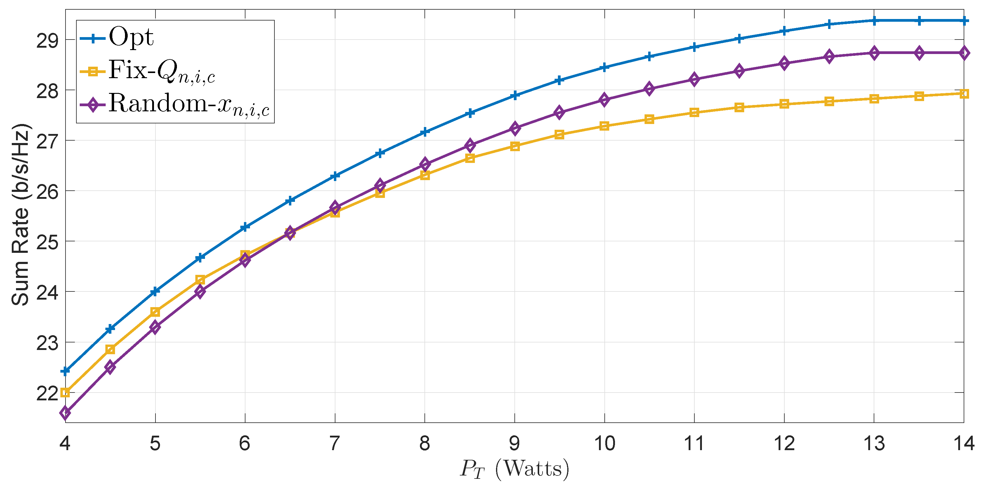
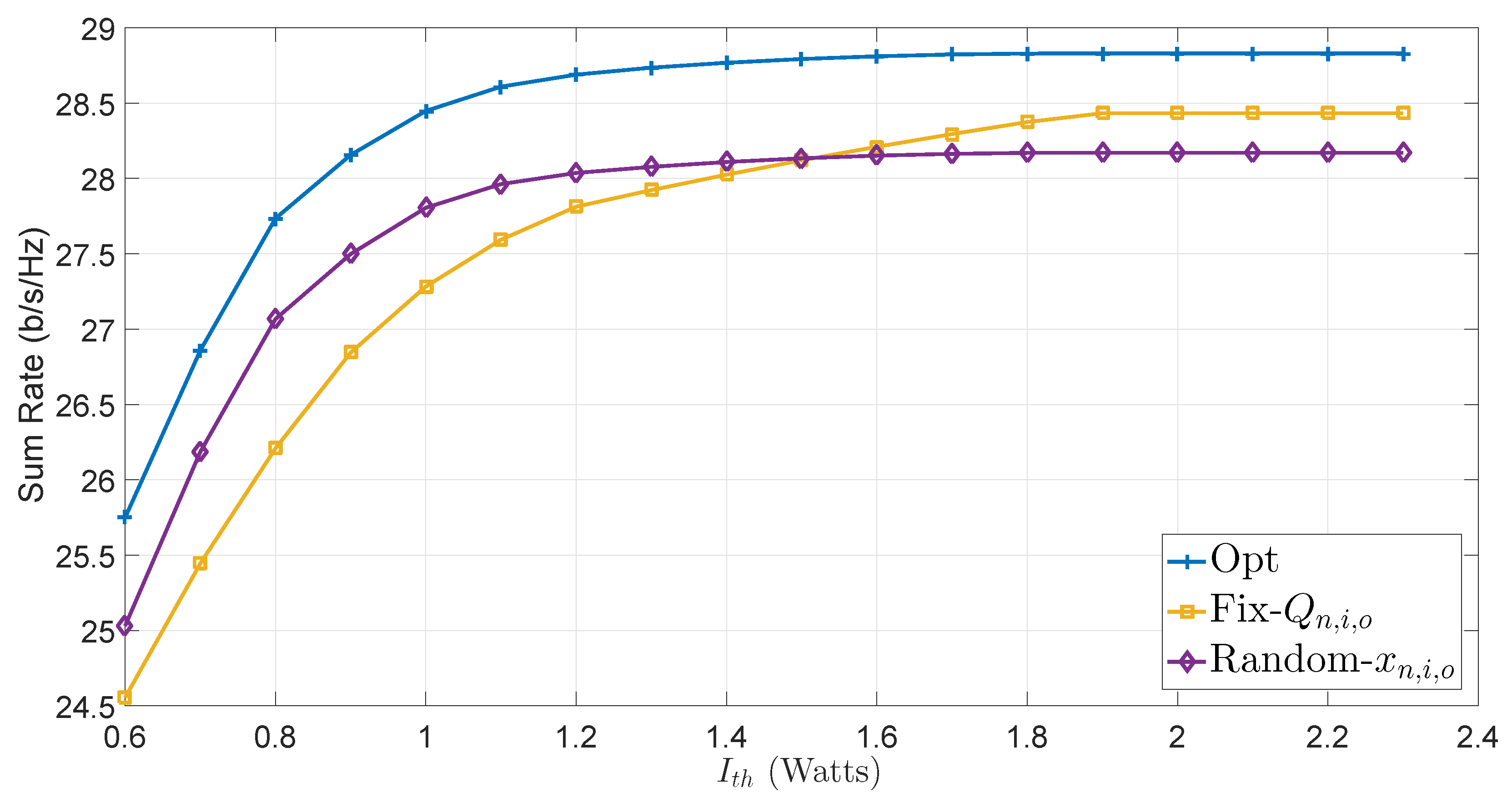
The effect of $P_T$ on the sum rate of all the schemes is shown in Figure 2. It can be seen that an increase in $P_T$ generally results in increasing the sum rate for all the schemes. However, after a certain point, the positive impact of increase in $P_T$ on the rate reduces. This is because at this point the interference generated by user pairs with better channels have reached $I_{th}$. Thus, no more power is allocated to these pairs and the extra power is assigned to comparatively bad users. It can be seen that in Opt when $P_T\ge 13$ the sum rate does not change at all. At this point, the interference of all user pairs has become equal to $I_{th}$. Hence, when $P_T$ increases, the power allocated to the users remains unchanged. A similar trend can be seen in the case of Random-$x_{n,i,c}$. The figure shows that Opt outperforms all the other schemes. When $P_T$ is increased the interference generated by a user pair may become equal to $I_{th}$. With further increases the interference of more and more user pairs become equal to the threshold. Hence, no more power can be allocated for the transmissions of these users. In the case of $Opt$ and $Random-x_{n,i,c}$, when the interference of pairs that offer higher rates become equal to the threshold the remaining power is allocated to the users with comparatively bad channel gains. However, Fix-$Q_{n,i,c}$ is incapable of distributing the remaining power to the other user pairs. Thus, an increase in $P_T$ is more beneficent for $Opt$ and Random-$x_{n,i,c}$ as compared to Fix-$Q_{n,i,c}$. Thus, for $P_T<6.5$, the sum rate provided by Fix-$Q_{n,i,c}$ is greater than Random-$x_{n,i,c}$. When $P_T>6.5$, the Fix-$Q_{n,i,c}$ provides worst performance.

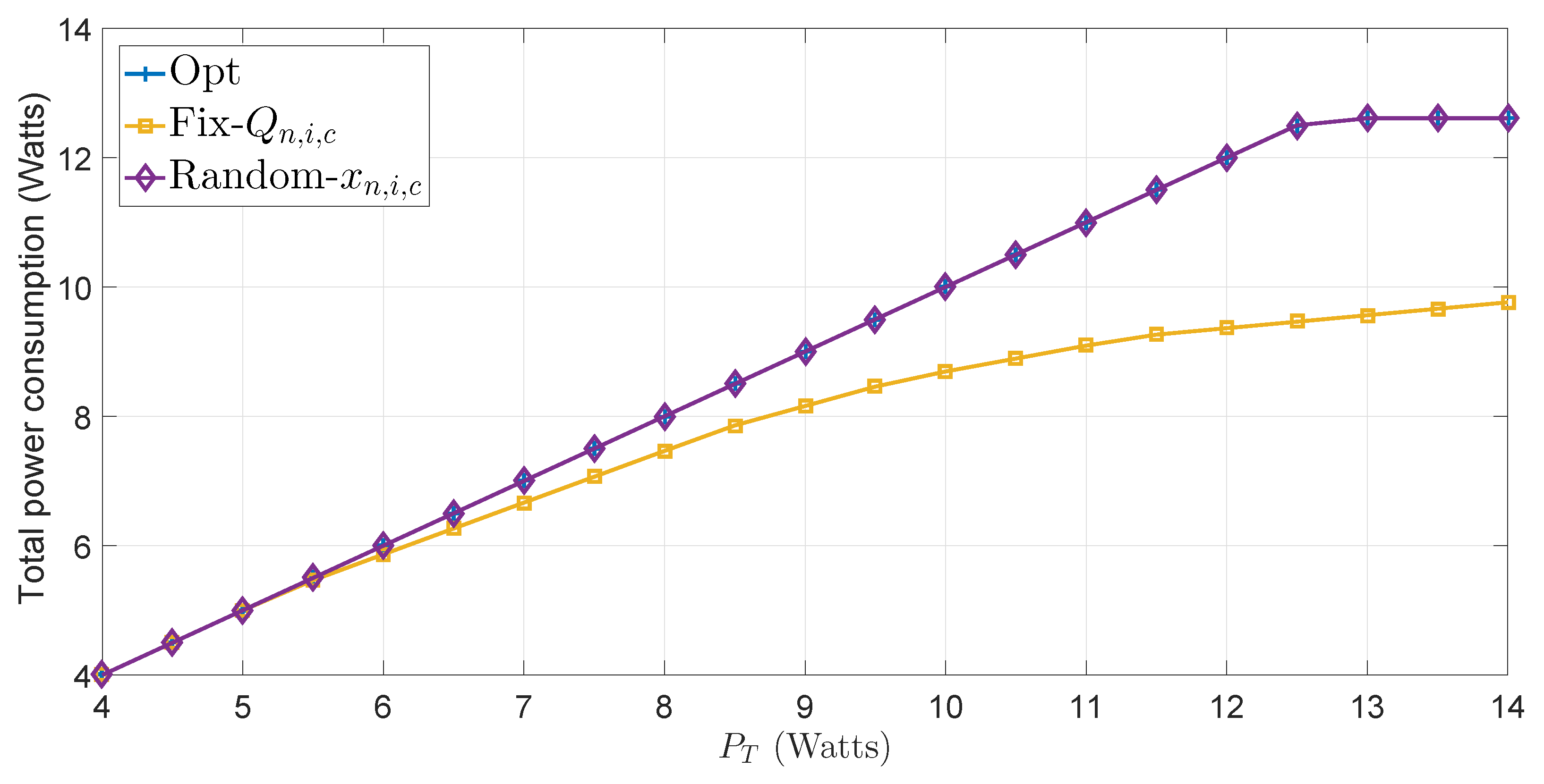
The impact on the power consumption of each scheme for changing $P_T$ is presented in Figure 3. The transmission power of each scheme increase with $P_T$ until the interference generated by each user pair becomes equal to $I_{th}$. After this point, an increase in $P_T$ has no effect. The power consumption of Opt at this point is equal to Random-$x_{n,i,c}$. However, Figure 2 shows that the sum rate provided by Opt is greater than these schemes. Thus, it could be concluded that Opt is more efficient than Random-$x_{n,i,c}$. In the case of Fix-$Q_{n,i,c}$, when $P_T\le 5.5$, the scheme takes advantage of full power available. For $P_T>5.5$, the interference of some pairs become equal to $I_{th}$. In this situation, all the other schemes allocate the extra power to other user pairs and so are capable of taking advantage of the increase in $P_T$. However, in the case of Fix-$x_{n,i,c}$, this extra power is not allocated to any other user pair, thus resulting in poor performance as compared to the other schemes.

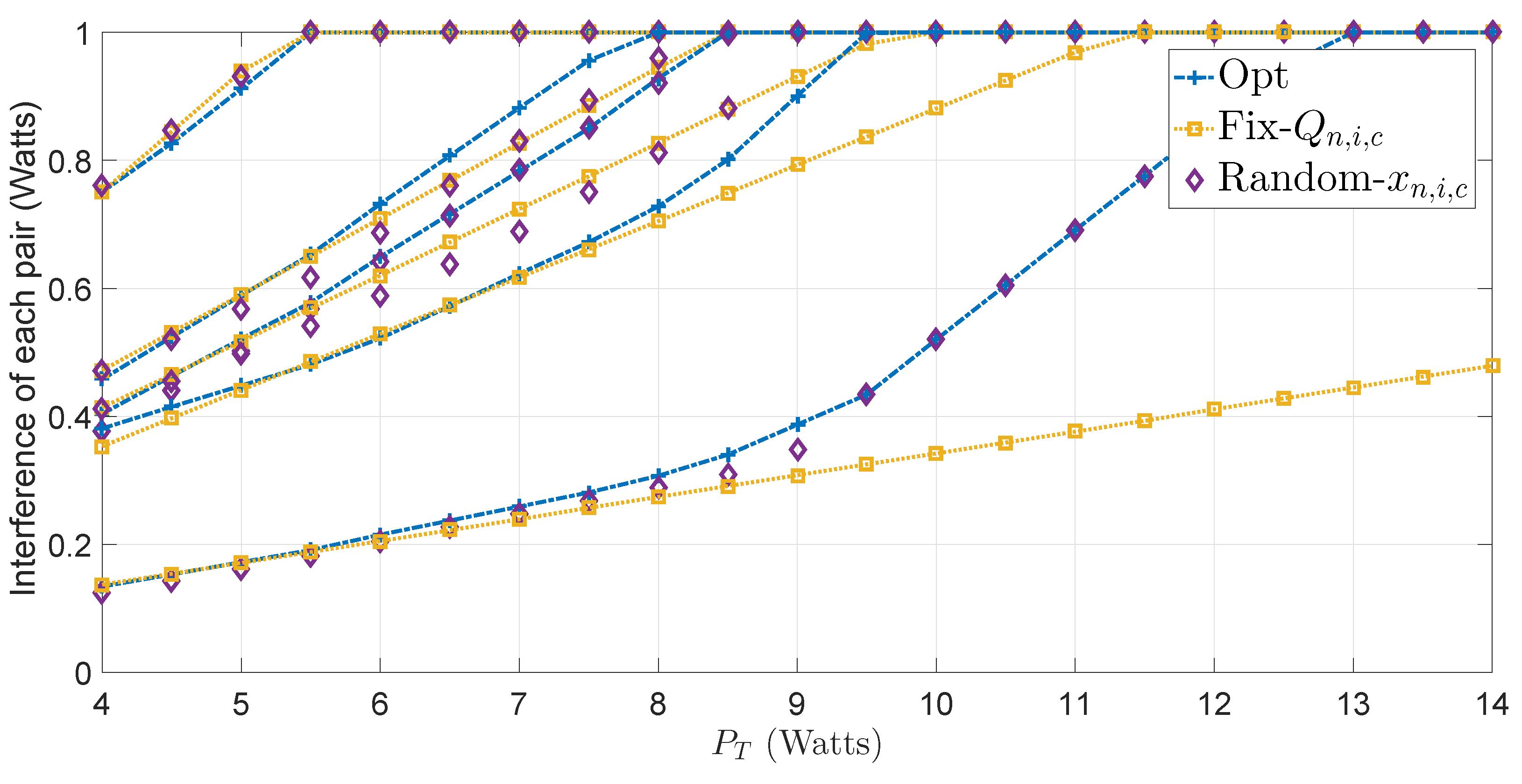
The interference of each user pair in each scheme is compared in Figure 4. In all the cases where $Q_{n,i,c}$ is optimized, when the interference of a user pair reaches threshold an increase in the slope of some other pair’s curve is observed. This shows that the power allocated to this user pair has increased because the extra power is now being allocated to this pair. However, in the case of Fix-$Q_{n,i,c}$, the interference of each pair increases at a constant rate with $P_T$. This is because in this scheme the extra power is wasted and each pair just gets its own equal share from the increased vale of power budget.

Figure 5 shows the impact of $I_{th}$ on the sum rate. Initially, an increase in $I_{th}$ results in increasing the sum rate of each scheme. At these points, the transmit power of the users are upper bounded by $I_{th}$. Thus, when $I_{th}$ increase, the transmit power of each pair also increases. This results in enhancing the sum rate. After a certain point, an increase in $I_{th}$ has no impact on the sum rate. At these points, each scheme is already transmitting with full available power. Hence, no more power is available for transmission. It can be seen that Opt out performs all the other schemes. For $I_{th}<1.5$, the worst performance is provided by Fix-$Q_{n,i,c}$ because the power allocation to user pairs is bounded by $I_{th}$ and the scheme cannot reallocated the extra power to the pairs that generate less interference. However, when $I_{th}>1.5$ the Fix-$Q_{n,i,c}$ performs better than Random-$x_{n,i,c}$. At larger values of $I_{th}$, the power allocation of less user pairs is bounded by $I_{th}$ so Fix-$Q_{n,i,c}$ can take advantage of the available power and so the sum rate of Fix-$Q_{n,i,c}$ at these points surpasses Random-$x_{n,i,c}$.

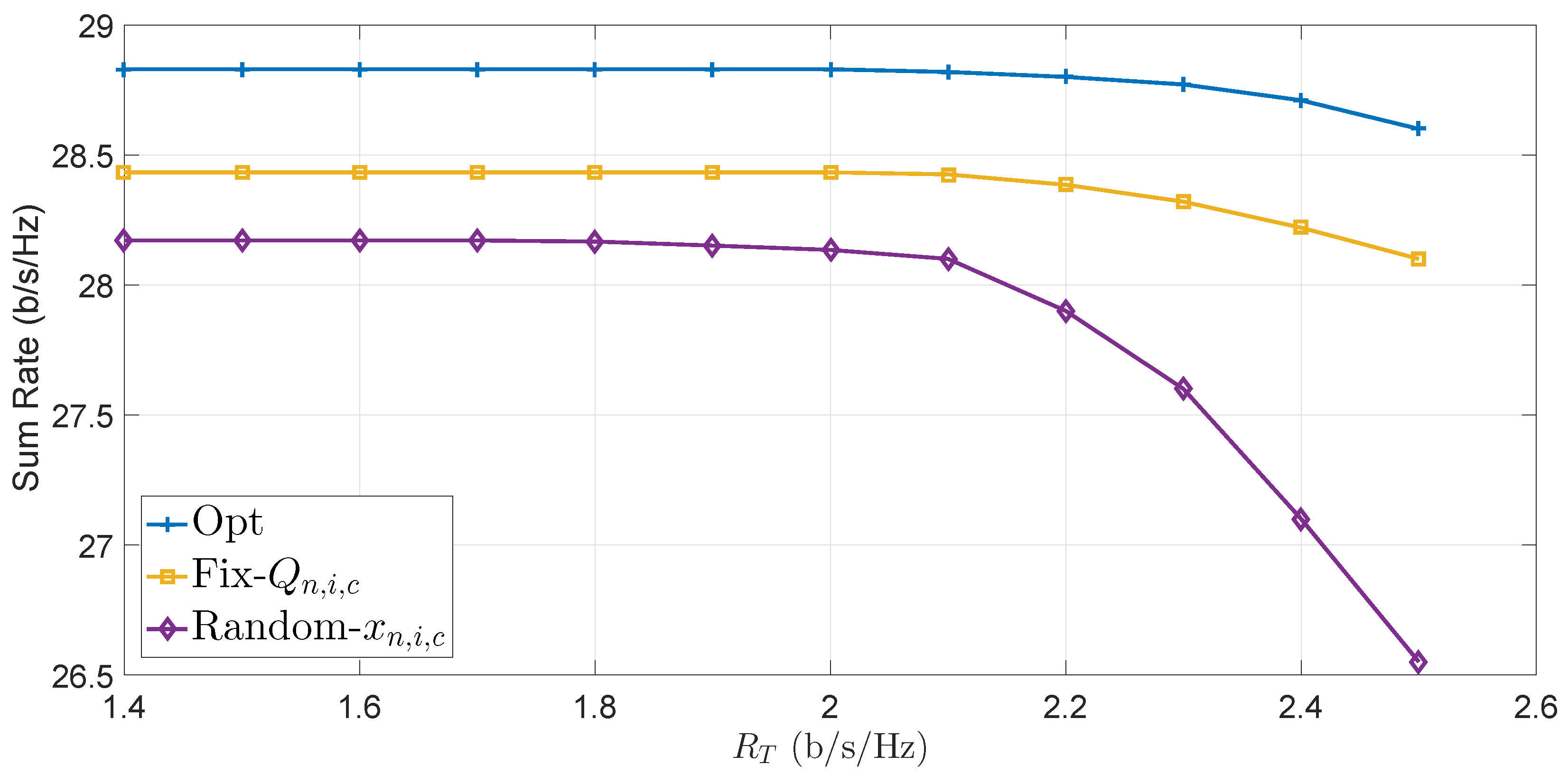
The sum rate of each scheme also depends on $R_T$, as shown in Figure 6. To make the impact of $R_T$ more prominent, we considered $I_{th}=2W$, so that the power allocation is not bounded by interference. For small values, increasing $R_T$ has no impact on the sum rate because the rate of each user is already greater than $R_T$. However, after a certain point when $R_T$ is further increased the sum rate decreases as a result. This is because at these points to satisfy the rate constraint the power allocation of the weak users is increased. The same amount of power results in larger value of rate for a user with good channel condition as compared to a user with low value of channel gain, thus, when power allocated to a user with better channel conditions is reduced and is allocated to the user with poor channel, the sum rate decreases. Further, the Opt offers larger values of sum rate compared to all other schemes for each $R_T$. The Random-$x_{n,i,c}$ has the worst performance because in random pairing if two users with poor channel conditions are paired together. This pair would require a large amount of power to meet $R_T$. Thus, less power would be available for the user pairs that can offer high rates. Hence, with an increase in $R_T$ the rate of Random-$x_{n,i,c}$ is affected more as compared to the other schemes.

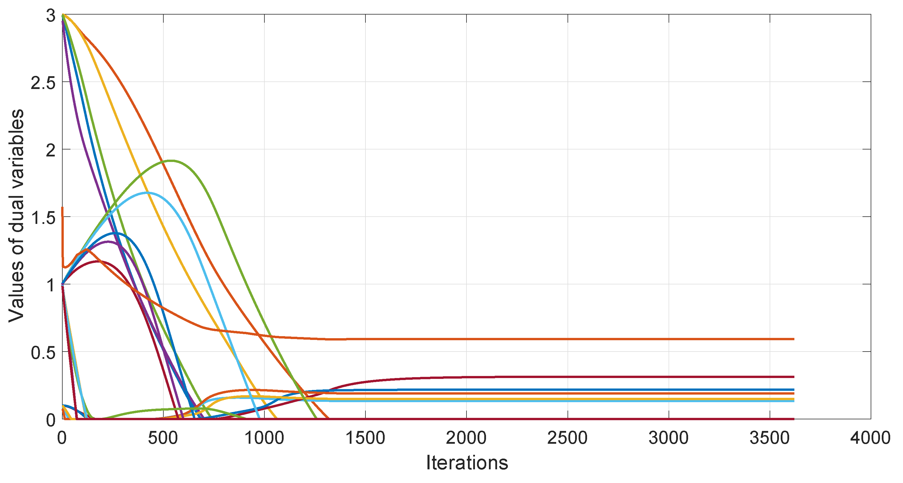
The convergence behavior of all the dual variables is presented in Figure 7. It can be seen that all the dual variables converge within a reasonable number of iterations.

5. Conclusions

In this study, we considered the problem of maximizing the sum rate of the secondary users in a NOMA based CR system. The constraints of power budget, interference temperature, QoS requirement of each user and NOMA power gap were taken into account. For the solution, we first transformed the non-convex optimization problem into a convex form. We proposed a dual decomposition based solution for power allocation. An efficient algorithm for user pairing and channel allocation was also designed. The simulations compared the performance of the proposed scheme with two scenarios. In the first case, the power allocated to each user pair was optimized for random user pairing and channel allocation (Random-$x_{n,i,c}$). In the second scenario, fix amount of power was allocated to each pair where the user pairing and channel allocation was carried out as in the proposed Opt scheme. In both cases, the allocated power to a pair was distributed among the user as in Opt. The results show that at small values of available power or high interference threshold the advantages of intelligent user pairing and channel allocation surpass optimal power allocation to the pairs. However, at low interference threshold or high power budget the optimal power allocation to each pair provides better performance. In addition, as the rate requirement of users in the system increases the gap in the rates offered by Fix-$Q_{n,i,c}$ and Random-$x_{n,i,c}$ also increases. At higher values of $R_T$, Fix-$Q_{n,i,c}$ provides much better performance as compared to Random-$x_{n,i,c}$. The results show that the proposed Opt scheme offers more rate as compared to the other cases. In future works, we will incorporate some intelligent algorithms [33,34] into the considered system, in order to enhance the system performance.

References

- Xie, H.; Gao, F.; Zhang, S.; Jin, S. A unified transmission strategy for TDD/FDD massive MIMO systems with spatial basis expansion model. IEEE Trans. Veh. Technol. 2016, 66, 3170–3184. [Google Scholar] [CrossRef]
- Xie, H.; Gao, F.; Jin, S.; Fang, J.; Liang, Y. Channel estimation for TDD/FDD massive MIMO systems with channel covariance computing. IEEE Trans. Wirel. Commun. 2018, 17, 4206–4218. [Google Scholar] [CrossRef]
- Wang, Z.Y.; Yu, H.Y.; Wang, D.M. Channel and Bit Adaptive Power Control Strategy for Uplink NOMA VLC Systems. Appl. Sci. 2019, 9, 220. [Google Scholar] [CrossRef]
- Marcano, A.S.; Christiansen, H.L. Performance of non-orthogonal multiple access (NOMA) in mm-wave wireless communications for 5G networks. In Proceedings of the International Conference on Computing, Networking and Communications (ICNC), Santa Clara, CA, USA, 26–29 January 2017; pp. 969–974. [Google Scholar]
- Althunibat, S.; Mesleh, R.; Qaraqe, K. Quadrature index modulation based multiple access scheme for 5G and beyond. IEEE Commun. Lett. 2019. [Google Scholar] [CrossRef]
- Althunibat, S.; Mesleh, R.; Rahman, T.F. A novel uplink multiple access technique based on index-modulation concept. IEEE Trans. Commun. 2019, 67, 4848–4855. [Google Scholar] [CrossRef]
- Wu, Y.; Attang, E.; Atkin, G.E. Low complexity NOMA system with combined constellations. IEEE Wirel. Commun. Lett. 2019. [Google Scholar] [CrossRef]
- Ali, A.; Baig, A.; Awan, G.M.; Khan, W.U.; Ali, Z.; Sidhu, G.S. Efficient resource management for sum capacity maximization in 5G NOMA systems. Appl. Syst. Innov. 2019, 2, 27. [Google Scholar] [CrossRef]
- Fang, F.; Cheng, J.; Ding, Z. Joint energy efficient subchannel and power optimization for a downlink NOMA heterogeneous network. IEEE Trans. Veh. Technol. 2019, 68, 1351–1364. [Google Scholar] [CrossRef]
- Liu, M.; Song, T.; Hu, J.; Yang, J.; Gui, G. Deep learning-inspired message passing algorithm for efficient resource allocation in cognitive radio networks. IEEE Trans. Veh. Technol. 2019, 68, 641–653. [Google Scholar] [CrossRef]
- Gao, Y.; Xiao, Y.; Wu, M.; Xiao, M. Energy efficient power allocation with demand side coordination for OFDMA downlink transmissions. IEEE Trans. Wirel. Commun. 2019, 18, 2141–2155. [Google Scholar] [CrossRef]
- Cui, J.; Ding, Z.; Fan, P. A novel power allocation scheme under outage constraints in NOMA systems. IEEE Signal Process. Lett. 2016, 23, 1226–1230. [Google Scholar] [CrossRef]
- Yang, Z.; Ding, Z.; Fan, P.; Dhahir, N.A. A general power allocation scheme to guarantee quality of service in down–link and uplink NOMA systems. IEEE Trans. Wirel. Commun. 2016, 15, 7244–7257. [Google Scholar] [CrossRef]
- Zhang, Y.; Wang, H.M.; Zheng, T.X.; Yang, Q. Energy-efficient transmission design in non-orthogonal multiple access. IEEE Trans. Veh. Technol. 2017, 66, 2852–2857. [Google Scholar] [CrossRef]
- Feng, Y.; Yan, S.; Yang, Z.; Yang, N.; Yuan, J. Beamforming design and power allocation for secure transmission with NOMA. IEEE Trans. Wirel. Commun. 2019, 18, 2639–2651. [Google Scholar] [CrossRef]
- Choi, J. Power allocation for max-sum rate and max-min rate proportional fairness in NOMA. IEEE Commun. Lett. 2016, 20, 2055–2058. [Google Scholar] [CrossRef]
- Ali, Z.; Sidhu, G.A.S.; Waqas, M.; Gao, F. On fair power optimization in nonorthogonal multiple access multiuser networks. Emerg. Telecommun. Technol. 2018, 29, 3540. [Google Scholar] [CrossRef]
- Zhou, F.; Beaulieu, N.C.; Li, Z.; Si, J.; Qi, P. Energy-efficient optimal power allocation for fading cognitive radio channels: Ergodic capacity, outage capacity, and minimum-rate capacity. IEEE Trans. Wirel. Commun. 2015, 15, 2741–2755. [Google Scholar] [CrossRef]
- Quach, T.X.; Tran, H.; Uhlemann, E.; Kaddoum, G.; Tran, Q.A. Power allocation policy and performance analysis of secure and reliable communication in cognitive radio networks. Wirel. Netw. 2019, 25, 1477–1489. [Google Scholar] [CrossRef]
- Yin, C.; Palacios, E.G.; Vo, N.S.; Duong, T.Q. Cognitive heterogeneous networks with multiple primary users and unreliable backhaul connections. IEEE Access 2018, 7, 3644–3655. [Google Scholar] [CrossRef]
- Zhang, J.; Nguyen, N.P.; Zhang, J.; Palacios, E.G.; Le, N.P. Impact of primary networks on the performance of energy harvesting cognitive radio networks. IET Commun. 2016, 10, 2559–2566. [Google Scholar] [CrossRef] [Green Version]
- Wei, Z.; Ng, D.W.K.; Yuan, J.; Wang, H.M.; Jin, S. Optimal resource allocation for power-efficient MC-NOMA with imperfect channel state information. IEEE Trans. Commun. 2017, 65, 3944–3961. [Google Scholar] [CrossRef]
- Wei, Z.; Ng, D.W.K.; Yuan, J. Power-efficient resource allocation for MC-NOMA with statistical channel state information. In Proceedings of the IEEE Global Communications Conference (GLOBECOM), Washington, DC, USA, 4–8 December 2016; pp. 1–6. [Google Scholar]
- Lei, L.; Yuan, D.; Ho, C.K.; Sun, S.J. Power and channel allocation for non-orthogonal multiple access in 5G systems: Tractability and computation. IEEE Trans. Wirel. Commun. 2016, 15, 8580–8594. [Google Scholar] [CrossRef]
- Ali, Z.; Sidhu, G.A.S.; Waqas, M.; Gao, F.; Jin, S. Achieving energy fairness in multiuser uplink CR transmission. In Proceedings of the IEEE Wireless Communications and Networking Conference, Doha, Qatar, 3–6 April 2016; pp. 1–6. [Google Scholar]
- Wang, S.; Shi, W.; Wang, C. Energy-efficient resource management in OFDM-based cognitive radio networks under channel uncertainty. IEEE Trans. Commun. 2015, 63, 3092–3102. [Google Scholar] [CrossRef]
- Pao, W.C.; Chen, Y.F.; Chuang, S.Y. Efficient power allocation schemes for OFDM-based cognitive radio systems. AEU Int. J. Electron. Commun. 2011, 65, 1054–1060. [Google Scholar] [CrossRef]
- Zeng, M.; Tsiropoulos, G.I.; Dobre, O.A.; Ahmed, M.H. Power allocation for cognitive radio networks employing non-orthogonal multiple access. In Proceedings of the IEEE Global Communications Conference (GLOBECOM), Washington, DC USA, 4–8 December 2016. [Google Scholar]
- Zabetian, N.; Baghani, M.; Mohammadi, A. Rate optimization in NOMA cognitive radio networks. In Proceedings of the International Symposium on Telecommunications (IST), Tehran, Iran, 27–28 September 2016; pp. 62–65. [Google Scholar]
- Saito, Y.; Kishiyama, Y.; Benjebbour, A.; Nakamura, T.; Li, A.; Higuchi, K. Non-orthogonal multiple access (NOMA) for cellular future radio access. In Proceedings of the Vehicular Technology Conference (VTC Spring), Dresden, Germany, 2–5 June 2013. [Google Scholar]
- Boyd, S.; Vandenberghe, L. Convex Optimization; Cambridge University Press: Cambridge, UK, 2004. [Google Scholar]
- Boyd, S.; Mutapcic, A. Subgradient Methods Notes for EE364; Winter 2006-07; Standford University: Stanford, CA, USA, 2006. [Google Scholar]
- Xia, J. Intelligent Secure Communication for Internet of Things with Statistical Channel State Information of Attacker. IEEE Access 2019, PP, 1–10. [Google Scholar] [CrossRef]
- Liu, G. Deep Learning Based Channel Prediction for Edge Computing Networks Towards Intelligent Connected Vehicles. IEEE Access 2019, 7, 114487–114495. [Google Scholar] [CrossRef]
Figure 1.
Considered system model.
Figure 2.
Impact of on sum rate for 3 different techniques.
Figure 3.
VS power consumption of all the considered techniques.
Figure 4.
Effect of increasing on the interference generated by each user pair in the system.
Figure 5.
A comparison of sum rate offered by each scheme for increasing .
Figure 6.
Impact of increasing on the sum rate of the techniques.
Figure 7.
Convergence of dual variables.
© 2019 by the authors. Licensee MDPI, Basel, Switzerland. This article is an open access article distributed under the terms and conditions of the Creative Commons Attribution (CC BY) license (http://creativecommons.org/licenses/by/4.0/).
Share and Cite
MDPI and ACS Style
Ali, Z.; Rao, Y.; Khan, W.U.; Sidhu, G.A.S. Joint User Pairing, Channel Assignment and Power Allocation in NOMA based CR Systems. Appl. Sci. 2019, 9, 4282. https://0-doi-org.brum.beds.ac.uk/10.3390/app9204282
AMA Style
Ali Z, Rao Y, Khan WU, Sidhu GAS. Joint User Pairing, Channel Assignment and Power Allocation in NOMA based CR Systems. Applied Sciences. 2019; 9(20):4282. https://0-doi-org.brum.beds.ac.uk/10.3390/app9204282
Chicago/Turabian StyleAli, Zain, Yanyi Rao, Wali Ullah Khan, and Guftaar Ahmad Sardar Sidhu. 2019. "Joint User Pairing, Channel Assignment and Power Allocation in NOMA based CR Systems" Applied Sciences 9, no. 20: 4282. https://0-doi-org.brum.beds.ac.uk/10.3390/app9204282
Note that from the first issue of 2016, this journal uses article numbers instead of page numbers. See further details here.