Deep Convolutional Neural Network-Based Approaches for Face Recognition


1
Computer Science Department, Faculty of Computing and Information Technology, King Abdulaziz University, Jeddah 21589, Saudi Arabia
2
Electrical Engineering Department, Faculty of Engineering at Shoubra, Benha University, Cairo 11629, Egypt
*
Author to whom correspondence should be addressed.
Appl. Sci. 2019, 9(20), 4397; https://0-doi-org.brum.beds.ac.uk/10.3390/app9204397
Submission received: 1 September 2019
/
Revised: 9 October 2019
/
Accepted: 14 October 2019
/
Published: 17 October 2019
(This article belongs to the Section Computing and Artificial Intelligence)
Abstract
:Face recognition (FR) is defined as the process through which people are identified using facial images. This technology is applied broadly in biometrics, security information, accessing controlled areas, keeping of the law by different enforcement bodies, smart cards, and surveillance technology. The facial recognition system is built using two steps. The first step is a process through which the facial features are picked up or extracted, and the second step is pattern classification. Deep learning, specifically the convolutional neural network (CNN), has recently made commendable progress in FR technology. This paper investigates the performance of the pre-trained CNN with multi-class support vector machine (SVM) classifier and the performance of transfer learning using the AlexNet model to perform classification. The study considers CNN architecture, which has so far recorded the best outcome in the ImageNet Large-Scale Visual Recognition Challenge (ILSVRC) in the past years, more specifically, AlexNet and ResNet-50. In order to determine performance optimization of the CNN algorithm, recognition accuracy was used as a determinant. Improved classification rates were seen in the comprehensive experiments that were completed on the various datasets of ORL, GTAV face, Georgia Tech face, labelled faces in the wild (LFW), frontalized labeled faces in the wild (F_LFW), YouTube face, and FEI faces. The result showed that our model achieved a higher accuracy compared to most of the state-of-the-art models. An accuracy range of 94% to 100% for models with all databases was obtained. Also, this was obtained with an improvement in recognition accuracy up to 39%.
1. Introduction
In the past few years, the field of machine learning has undergone some major developments. One important advancement is a technique known as “deep learning” that aims to model the high-level data abstractions by employing deep networked architectures composed of multiple linear/non-linear transformations. Deep learning systems are intelligent systems that mimic the workings of a human brain in representing complex data from real-world scenarios, and help in making intelligent decisions. Deep learning, also known as deep structured learning or hierarchical learning, belongs to the family of machine learning methods which are based on understanding data representation. It has made a remarkable impact in computer vision performance previously unattainable on many tasks such as image classification and object detection. Deep learning is applied in research concerning graphical modeling, pattern recognition, signal processing [1], computer vision [2], speech recognition [3], language recognition [4,5], audio recognition [6], and face recognition (FR) [7]. In biometrics, deep learning can be used to represent the unique biometric data and make improvements in the performance of many authentication and recognition systems.
Face recognition (FR) technology is identified as an active area of research in recent years because of the rise in security demands and the potential of the technology in law enforcement and commercial use [7]. FR contains two operational modes. First, verification mode is known as one-to-one matching in biometrics. The verification operational mode is used to pick out a face out of many faces in a face database to find out whether the face details belong to a particular person. Second, the identification mode is known as one-to-many matching. Identification involves taking the individual and comparing their biometrics to a database of possible identities. FR technology consists of four stages, which include face detection, alignment, representation (facial feature extraction), and classification [8]. In the FR system, the main challenge is the feature representation scheme used to extract features, using the better method for representation, for a given biometric trait. Feature extraction is one of the most important steps for image classification. Extracting features means retaining the most important information, which is required for classification. There are many feature extraction procedures that have been proposed for use in a biometric system, including principal component analysis (PCA) [9], independent component analysis (ICA) [10], local binary patterns (LBP) [11], and the histogram method [12]. Recently, the typical feature extraction approach used FR is deep learning, especially the convolution neural network (CNN), which shows remarkable advantages [13].
There are different approaches for using the CNN. First is learning the model from scratch. In this case, the architecture of the pre-trained model is used and trained according to the dataset. Second is using transfer learning with features from pre-trained CNN, in cases where the dataset is large. Finally, CNN can be used via transfer learning by keeping the convolutional base in its original form and then using its outputs to feed the classifier. The pre-trained model is used as a fixed feature extraction mechanism in cases where the dataset is small, or when the problem is similar to the one to be classified [14].
The goal of this paper was to apply pre-trained convolution neural network (CNN) approaches for FR and classification accuracy by analysis of FR performance using the pre-trained CNN (AlexNet and ResNet-50 models) for extracting features, followed by support vector machine (SVM) [15], and then using transfer learning with CNN (AlexNet model) for both feature extraction and classification. Different datasets were used in this study to evaluate the proposed FR systems, such as the ORL dataset [16], GTAV face dataset [17], Georgia Tech face [18], FEI dataset [19], labelled faces in the wild (LFW) [20], frontalized labeled faces in the wild (F_LFW) [21], and YouTube face dataset [22], in addition to a combined dataset called DB_Collection, collected from all datasets.
2. CNNs Preliminaries
Convolutional neural networks were initially proposed by LeCun in [23]. They have been successfully applied to computer vision problems, such as hand-written digit recognition [24]. CNNs have recently grown in popularity in the field of pattern classification. CNNs have outperformed traditional computer vision methods in image classification. A convolutional neural network is a sort of artificial neural network (ANN) inspired by the performance of visual recognition of objects by animals and human beings’ cortex, which is used for applications including systems recommender [25], video and image recognition [26], and natural processing of languages [27,28]. CNN architectures makes the explicit assumption that the inputs are images, which allows encoding of certain properties into the architecture. Neurons in CNN are 3D filters that activate depending on their inputs. They are connected only to a small region, called the receptive field [29], of a previous neuron’s activations. They compute a convolution operation between the connected inputs and their internal parameters, and they get activated depending on their output and a non-linearity function [30].
Convolutional neural network layers are divided into three types: the convolutional, pooling and, fully connected layers. Each layer plays a different role. The CNN architecture is shown in Figure 1.
Convolutional layer: Convolutional layer is known as the elemental development block for CNN. In CNN technology, it is crucial to understand that the layers’ parameters are made up of a set of learnable filters or neurons. These filters have a small receptive field, but they go all the way through the input volume. In the forward pass process, each individual filter goes across the width and height of the input volume, calculating the dot product from the filter entries and the input. The product of this computation is a two-dimensional activation map of that filter. Through this, the network learns filters created when it senses some particular type of feature at a spatial location within the feature-map input X, generating a feature map of weighted summations Y. Each of the neurons computes convolutions with small regions in X, shown in Equation (1) [23].
where yj ∈ Y, j = 1, 2, ..., D. D is the depth of the convolutional layer, and each filter wij is a 3D matrix of size [F × F × Cx]. Its size is determined by a chosen receptive field (F), and its feature-map input’s depth (Cx); for example, if the receptive field is five pixels and the feature-map input X is a [32 × 32 × 3] RGB image, then the filter’s size will be [5,5,3]. The filter’s size represents the number of weights that a neuron has connecting to a region in the input. The convolutional layer has the advantage of using the same neurons for each pixel in the layer to improve the system’s performance. In addition, this results in the reduction of the footprint’s memory making it efficient.
Pooling layers: Pooling layers are responsible for regulating the width by height dimensions by reducing the input volume spatial dimensions for the next convolutional layer without affecting the dimensional depth of the volume. The process performed by the pooling layer is also known as down-sampling or sub-sampling because the decrease of size results in simultaneous information loss that benefits the network. The reduction becomes less computational as the information progresses to the next pooling layers, and it also works against over-fitting. The most common strategies used in the pooling layer networks are max-pooling and average-pooling. In [31], a comprehensive theoretical analysis of the max pooling and average pooling is generated, whereas in [32] it has shown that max pooling can result in faster convergence of information, and the network picks the high-ranking features in the image thus enhancing generalization. Also, pooling layer possesses other variations such as stochastic pooling [33], spatial pyramid pooling [34], and def-pooling [35] that serves marked purposes.
Fully connected layers: Fully connected layers (FC) are where the levels of high reasoning are carried out. The filters and neurons in this layer are connected to all the activation in the previous layers, resulting in full connections as their name implies. The calculations in this level are done through the multiplication of matrix followed by the bias offset. FC layer goes through a process that converts the 2D feature map to the 1D feature vector. In addition, the vector formed in this process is either classified as classes for classification [36] or the feature vector undergoes further processing [37].
2.1. CNN Pre-Trained Models
In the convolution neural network, face representation extensively affects the performance of the FR system and has also become a focus of attention in the current FR research. In this study, we employed two pre-trained convolution neural networks. These networks were AlexNet and ResNet-50. These pre-trained CNN networks have been used to extract suitable image features and utilize them in the classification stage.
2.1.1. AlexNet
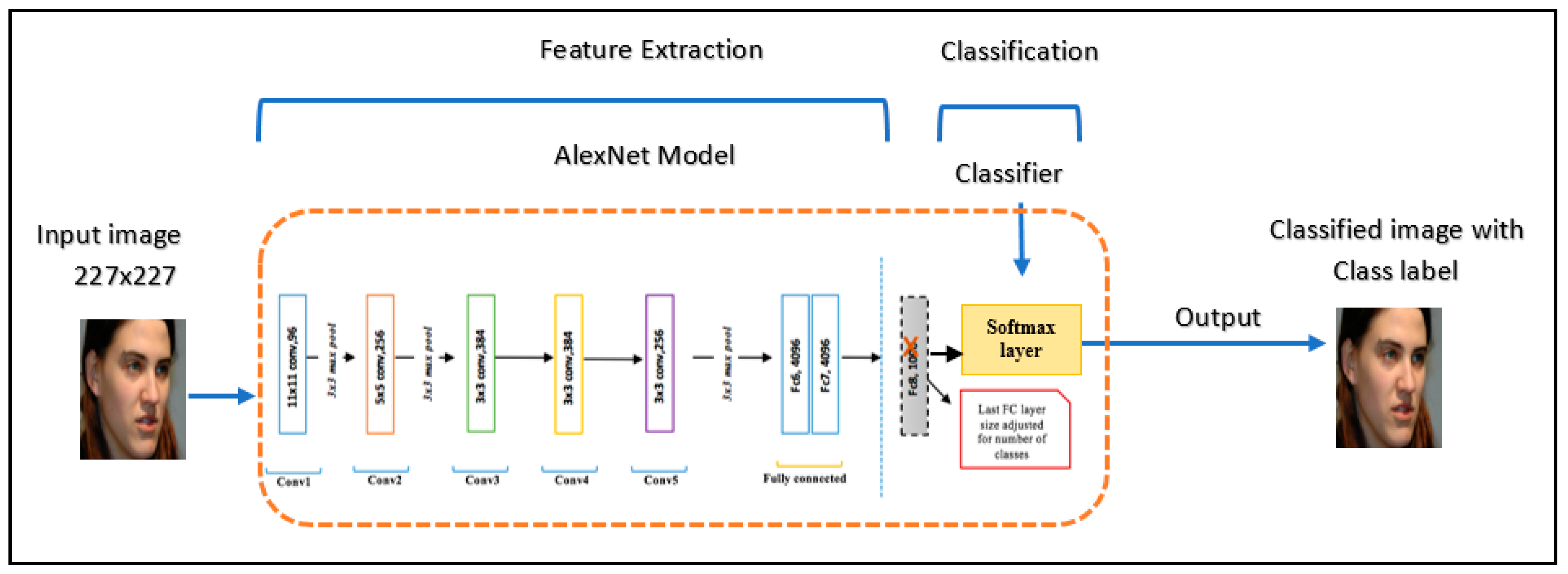
AlexNet, introduced by Krizhevsky et al. [36], was the first CNN to win the ImageNet challenge in 2012, with a top 5 error of 16.4%. The use of rectified linear units (ReLUs) was also introduced in AlexNet. As shown in Table 1, it includes five convolutional layers, three max pool layers, and three fully connected layers. This architecture uses a [227 × 227 × 3] image as an input. In AlexNet, a 4096-dimensional feature vector represents the 227 × 227 image.
2.1.2. ResNet-50
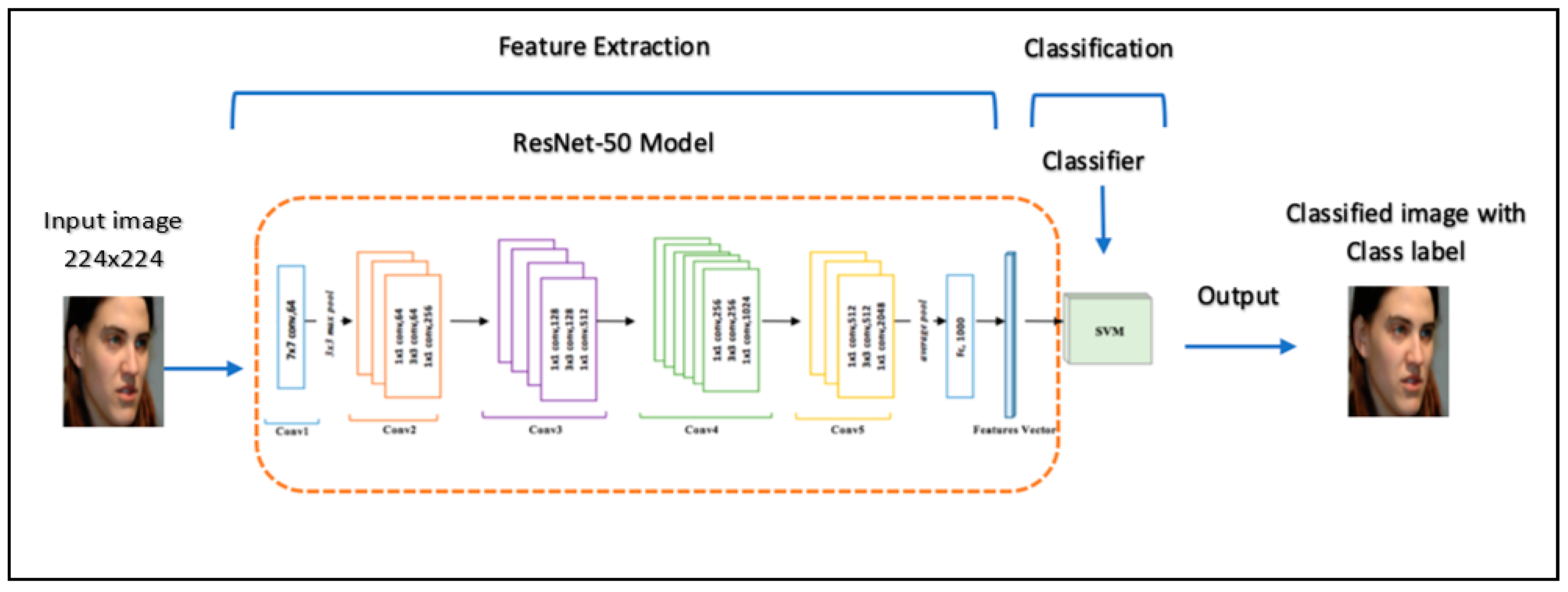
ResNet or deep residual networks [38], developed by Kaiming He et al., is one of the networks that are considered the latest and greatest in terms of using convolutional neural networks for image recognition. ResNet won the ImageNet Large-Scale Visual Recognition Challenge in 2015 (ILSVRC-15) with a top 5 error of 3.57%. In our study, we used ResNet-50 as shown in Table 2. It includes five convolutional layers. ResNet-50 architecture uses a [224 × 224 × 3] image as an input.
3. Related Work
Recently, convolutional neural networks have made great achievements in resolving different image processing problems for FR applications. Yu et al. [39] proposed a novel method called biometric quality assessment (BQA) for face images, investigating its applicability in FR applications. They used a light CNN with the max-feature-map units to make the BQA method more robust to noisy labels. Their studies have been explored further through experiments on the YouTube, FLW, and CASIA databases. The results of their experiments show a high degree of effectiveness of their proposed BQA method.
Sun et al. [40] conducted research on the potential use of hybrid deep learning for face verification. The researchers used, in particular, an experimental design involving a hybrid convolutional network (ConvNet) based on the restricted Boltzmann machine (RBM) model for purposes of face verification. The results showed that the hybrid deep learning achieved an excellent performance when it came to face verification as compared to the other commonly used methods. Singh and Om [41] used the deep convolutional neural network to identify the specific individuals from newborn infant datasets. The datasets used for their research contained 210 infants. Each infant consisted of 10 images with different facial expressions. They inferred that increasing the number of hidden layers does not increase the identification accuracy, and they also found that using a greater number of convolution layers tended to fit over the model, and that may also decrease the performance. Guo et al. [42] put forward a CNN-based model that meant to use both visible light image and near-infrared image to obtain facial recognition. Additionally, they created an adaptive score fusion strategy whose purpose was to significantly improve the performance. In comparison to the traditional deep learning procedure, this scheme can develop a robust face feature extraction model. When in use practically, it is robust to illumination variation. The researchers conducted a validity testing through various datasets. The results of the experiments indicated that the new model achieved enhanced performance. Hu et al. [43] investigated the performance of CNN on 2D and 3D FR systems. In their research, two CNN models were constructed—CNN-1 and CNN-2. The experiments of the study found a better accuracy on the CNN-2 model on both 2D and 3D face recognition. Also, the experimental results for CNN-2 showed an accuracy of 85.15% with the FRGCv2.0 dataset and 95% with the AT&T dataset. The results of their research showed that the CNN model is effective for facial images in 2D and 3D.
G. P. Nam et al. [44] proposed a CNN model named PSI-CNN for face recognition. The PSI-CNN model extracts untrained features from the image, then fuses these features with original feature maps. The results of the experiments are shown in terms of matching accuracy, with the model outperforming the model derived from the VGG-Face model. Also, PSI-CNN was able to maintain stable performance when tested on low-resolution images acquired from CCTV cameras. In case of change in image resolution and quality, PSI-CNN is robust. P. S. Prasad et al. [7] studied deep learning-based face representation for different face recognition challenges, such as misalignment, lower and upper face occlusions, illuminations, and different angles of head poses. They used two approaches—VGG-Face and lightened CNN. The AR face database used to evaluate the approaches’ results of the study showed that deep learning approaches provide a good result in terms of recognizing faces and pre-processing. Suleman Khan et al. [45] proposed a system for face recognition using portable smart glasses based on CNN. The detection process was performed using Haar-like features. The method archived detection rate at 98% using 3099 features. They used transfer learning from AlexNet for trained CNN model. The experiments of the study were conducted using 2500 images in a class. The results of the study showed that the accuracy of the system proposed was 98.5%. Chen Qin et al. [46] proposed a recognition algorithm based on deep CNNs. The algorithm contained face detection, face alignment, and feature extraction. The deep CNNs VGG16 was used to extract facial features. The experiments used the images of five angles (left, right, front, overlook, and look up). The experiment results showed that the algorithm achieved well on recognizing faces for cases of various poses in an indoor environment.
Menotti et al. [47] investigated two deep presentation processes composed of learning from CNN and weight adjustment, and iris spoof detection and fingerprints, the latter of which was the best approach for face detection and imaging. They admitted that indeed there was very limited experimental knowledge on the biometric spoofing at the sensors for deriving an outstandingly comprehensive spoofing detection framework for the face, iris, and fingerprint variations based on two major deep learning approaches. These approaches included a focus on learning of the weights of the networks through back propagation and learning of suitable convolutional network architectures for each of the CNN’s domains. Simón et al. [48] proposed a method on how to improve facial recognition. A multimodal facial recognition using the CNN’s systems is a good approach to facial recognition. They fused the modality-specific CNNs with histograms of Gabor ordinal measures (HOGOMs), local binary patterns (LBP), histograms of oriented gradients, and Haar-like features. The result of the approach significantly reduced the recognition error rate. Using more sophisticated computer systems will improve the process of deep learning. Similarly, there has been research-applied CNN, but this has been used on newborn FR [41].
Another study by Parkhi et al. [49] proposed VGG-Face system, which applied a 16-layer CNN trained on 2.6 million images and was shown to achieve even better results. Zhenyao et al. [50] used a deep network to “warp” faces into a canonical frontal view, after which the system learned CNN, which in turn classified the particular faces as those that matched a particular identity. For face verification, PCA on the network output in conjunction with an ensemble of SVMs was used. Also, Guo et al. [51] proposed an FR system based on CNN for feature extraction and SVM as a classifier. In order to enhance the performance of CNN, they used techniques for optimization to be training CNN. The model spends less time for training and gains a high recognition rate. The experiments in the study were conducted on the basis of the FERET and ORL dataset. The results of the experiments showed the system obtained and demonstrated a high recognition rate and less training time.
Even though CNNs have been used in FR technology dating back to 1997 [52], there are major improvements in that there are massive image datasets that are available and have revealed their power. A work used representatively for this approach is Deep-Face [13], whereby the researchers trained an eight-layer CNN architecture. These layers were distributed—the first three were conventional convolution-pooling-convolution layers, followed three layers that were locally connected and then two fully connected layers. It is crucial to note that the pooling layers had an effect of making learned features robust to local transformations but caused a miss in local texture details. The pooling layers were critical for object recognition because these objects were not properly aligned. It is, however, important to note that face images should be well-trained before CNN training. Deep-Face is trained on a large database of faces, which consists of 4 million facial images of 4000 subjects. The same study also proposed a 3D alignment approach that uses an affine camera model. This has realized an exemplary performance in both LFW and YouTube face benchmarks. Y. Sun et al. [53] proposed a CNN-based approach called DeepID. It is unlike DeepFace, which used one big CNN; instead, DeepID learns by training an ensemble of small CNNs and through building network fusion. In DeepID, each network includes four convolutional layers, three max-pooling layers, and two fully connected layers. DeepID achieved 97.45% accuracy on the LFW dataset. An extension work of DeepID is DeepID2 [54]. It trains CNN for verification and identification. DeepID2+ [55] has been proposed to improve the performance of DeepID and DeepID2. DeepID2+ net uses a larger training set than DeepID and DeepID2, and also improves the number of filters of all layers. DeepID2+ found that the face representations learned are sparse, selective, and robust. Recently, the success of deep convolutional neural networks has enhanced the performance of the FR model. Lu et al. [56] proposed a novel CNN-based approach called the Deep Coupled ResNet (DCR) model, which consists of one trunk network and two branch networks. The trunk network is used to extract discriminative features for face images of different resolutions. Then, the two branch networks are used to transform high-resolution (HR) images and corresponding images of the targeted low resolution (LR). The DCR model achieves better performance than the state-of-the-art models on the LFW and SCface datasets.
The reviewed related work shows that convolutional neural networks have been applied in different applications for feature extraction and classification, and many databases have been created to be used for this purpose. Table 3 summarizes the convolutional neural network application for face modality and face databases used in the related works presented in this section. Some research focuses on studying FR using convolutional neural networks, and they train the networks from scratch. In addition, some studies have conducted an experiment on one or two datasets. In our study, we used pre-trained convolutional neural networks and conducted all our experiment on seven datasets.
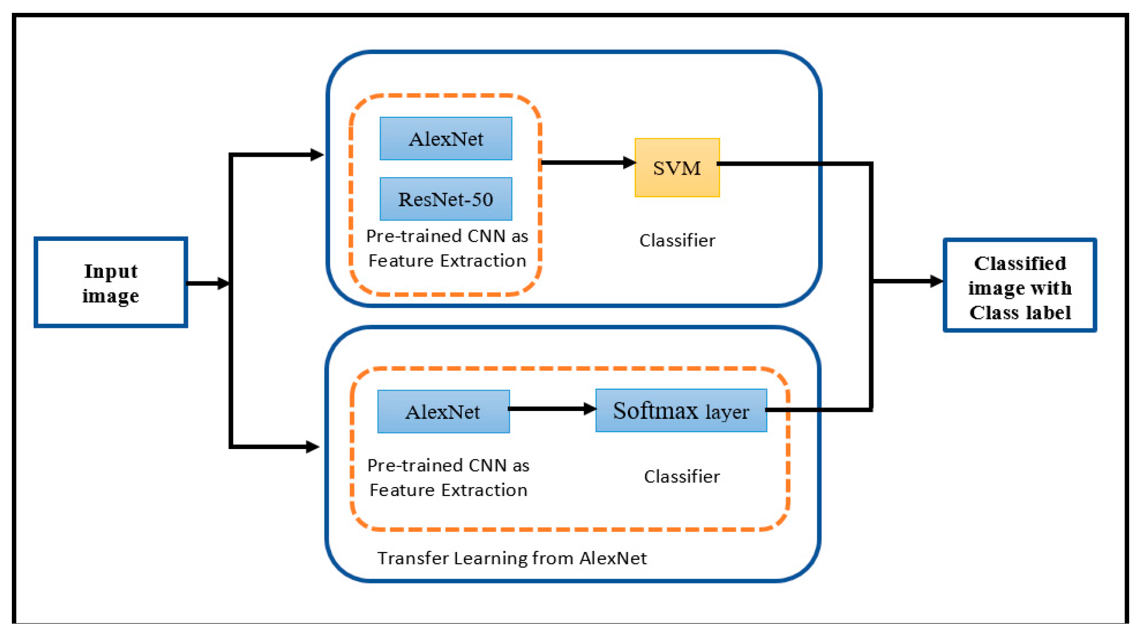
4. Methodology and Experiments
The main goal of this study was to investigate the FR performance through convolutional neural networks. For our system, we followed two approaches, as shown in Figure 2:
- First approach: Applying the pre-trained CNN for extracting features and support vector machine (SVM) for classification.
- Method 1: Pre-trained CNN AlexNet with SVM.
- Method 2: Pre-trained CNN ResNet-50 with SVM.
- Second approach: Applying transfer learning from AlexNet model for extracting features and classification.
In our study, we followed the following stages. First, the pre-processing stage, in which we resized each image to a suitable size for each CNN model and converted any grey images to RGB images. In the second stage, face representation, we employed two pre-trained convolution neural networks. These networks were AlexNet and ResNet-50. CNN networks have been used to extract suitable image features and utilize them in the following classification stage. Finally, the process of classifying faces occurred with different convolutional neural networks. First, we used two pre-trained convolution neural networks, AlexNet and ResNet-50, for extracting features, followed by an SVM as a classifier. Second, we applied transfer learning from the pre-trained AlexNet CNN for the classification task. Tests were conducted with different datasets. We then looked at the different results and analyzed the effectiveness of each approach and compared the results when using support vector machines (SVM) and transfer learning from pre-trained AlexNet. In our study, we used SVM as a classifier to recognize faces because of its observable classification result on nonlinear data. SVM has many advantages in solving pattern recognition problems and machine learning problems such as FR and function overfitting.
The SVM [15] classification is referred to as a process whereby the supervised binary classification method is used and when a training set is introduced, wherein the algorithm develops a hyperplane that maximizes the margin that exists between two input classes. For instance, considering linearly separate data with two distinct classes, the system can have numerous hyperplanes which separate two classes. SMVs identify the most ideal hyperplane that has a maximum margin between all available hyperplanes, whereby the margin is the distance difference between the hyperplane and the support vectors. In SVM, assuming that we represent the input/output sets as X and Y, the goal is to learn the function y = f (x, α), where α is the parameters of the function, and f can be defined as f (x, {w, b}) = sign (w × x + b). Thus, the goal is to find the best set of parameters w and b so that the margin is maximized. However, in the real world, the data are not always linear, and it is not possible to classify by a linear classifier, and thus the non-linear SVM classifier is proposed. The non-linear SVM comes with the kernel trick. The kernel trick is a very interesting and powerful tool. The selection of a suitable kernel for a given application or for a set of features is still an open problem. In this paper, the selected kernel function is a linear kernel function without any optimization, which means that linear kernel function does not have any parameters to optimize. In this study, we will not focus on investigating the strategies for SVM optimization.
4.1. Setting
All experiments were conducted using the platform of Windows with the configuration of Intel Core i7- CPU @ 2.7 GHz with 16 GB on NVIDIA GEFORCE GTX 1050TI. MATLAB 2018a tool was used to evaluate the method and perform the feature selection and classification task. As previously mentioned, before beginning the training process for the convolutional neural network architectures, a previous pre-processing is required. For all datasets, a rescale is applied to resize the images to a 227 × 227 as input for AlexNet and 224 × 224 as input for ResNet-50. The performance of the pre-trained convolutional neural network system is evaluated on the basis of the quality metric known as recognition accuracy. The accuracy is the fraction of the predicted labels that are correct.
Dataset Description
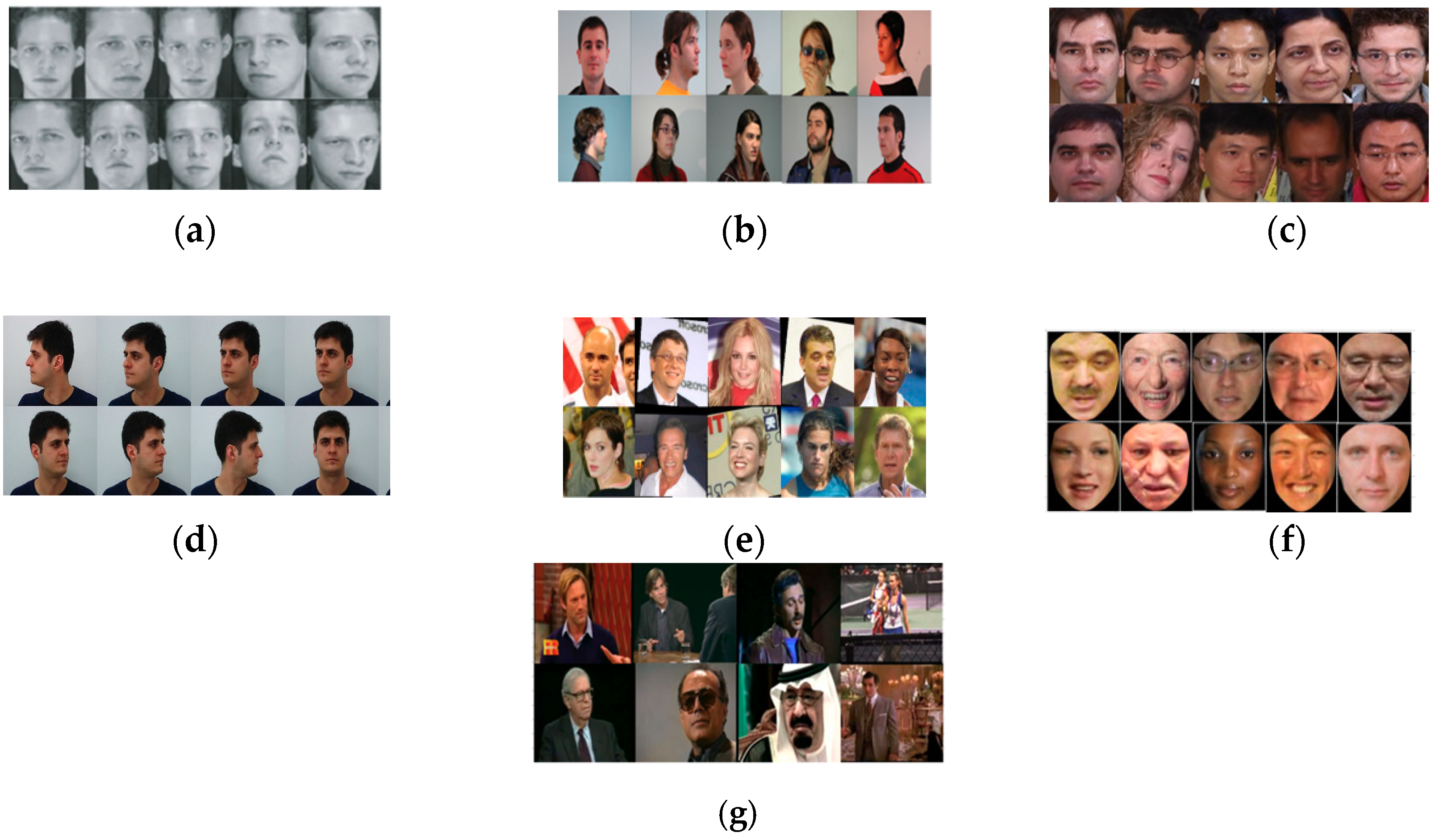
This section describes all datasets used in this study. Table 4 summarizes the data in each database used in the study. Some samples from all datasets are shown in Figure 3.
- ORL [16]: The database utilized in recognition experiments. It contains 10 unique images of 40 individuals, adding up to a total of 400 images that have different face angles, facial expressions, and facial details. The dataset has a collection at the Olivetti Research Laboratory at Cambridge University for some individuals.
- GTAV face database [17]: The database contains images for 44 individuals, which were taken on different pose views (0º, ±30º, ±45º, ±60º and 90º) for three illuminations (environment or natural light, strong light source from an angle of 45º, and an almost frontal mid-strong light source with environment or natural light). In our study, 34 images per each person in the dataset were chosen.
- Georgia Tech face database [18]: This database contains sets of images for 50 individuals, and there are 15 color pictures for each person. Most of the pictures were taken in two different sessions to consider the variations in illumination conditions, appearance, and facial expression. Also, the images in the datasets were taken at different orientations and scales.
- FEI face [19]: The database has 14 image sets for every individual among all the 200 people, totaling up to 2800 images. In our study, we chose frontal images for each individual. The total number of images that were chosen in the study was 400 images. In our experiment, we chose images for 50 individuals in a total of 700 images.
- Labeled faces in the wild (LFW) [20]: This dataset was designed for studying the problem of unconstrained face recognition. The dataset contains more than 13,000 images of faces collected from the web. Each face has been labeled with the name of the person pictured. A total of 1680 of the people pictured have two or more distinct photos in the dataset.
- YouTube face (YTF) [22]: The dataset contains 3425 videos collected from YouTube. The videos are a subset of the celebrities in the LFW. The videos contain 1595 individuals. In our study, we used images taken from video.
- DB_Collection: This dataset contains images combined from all datasets used in this study. We selected images for 30 people from each dataset, a total of 2880 images.
4.2. Experiments and Results
This section presents the experimental results that were obtained in face recognition using the three deep convolutional neural networks—AlexNet and ResNet-50 with SVM classifier, and transfer learning from AlexNet based on various standard datasets. The main three experiments in our study were conducted to compare the difference in performance between pre-trained CNN architectures. First, we evaluated the performance when extracting the learned image features from a pre-trained CNN AlexNet, followed by SVM as a classifier. Second, we extracted the learned image features from ResNet-50, followed by an SVM classifier. Third, we evaluated the performance when transfer learning from the AlexNet network was used for the classification task. The analysis and evaluation were carried out on the basis of the performance recognition accuracy.
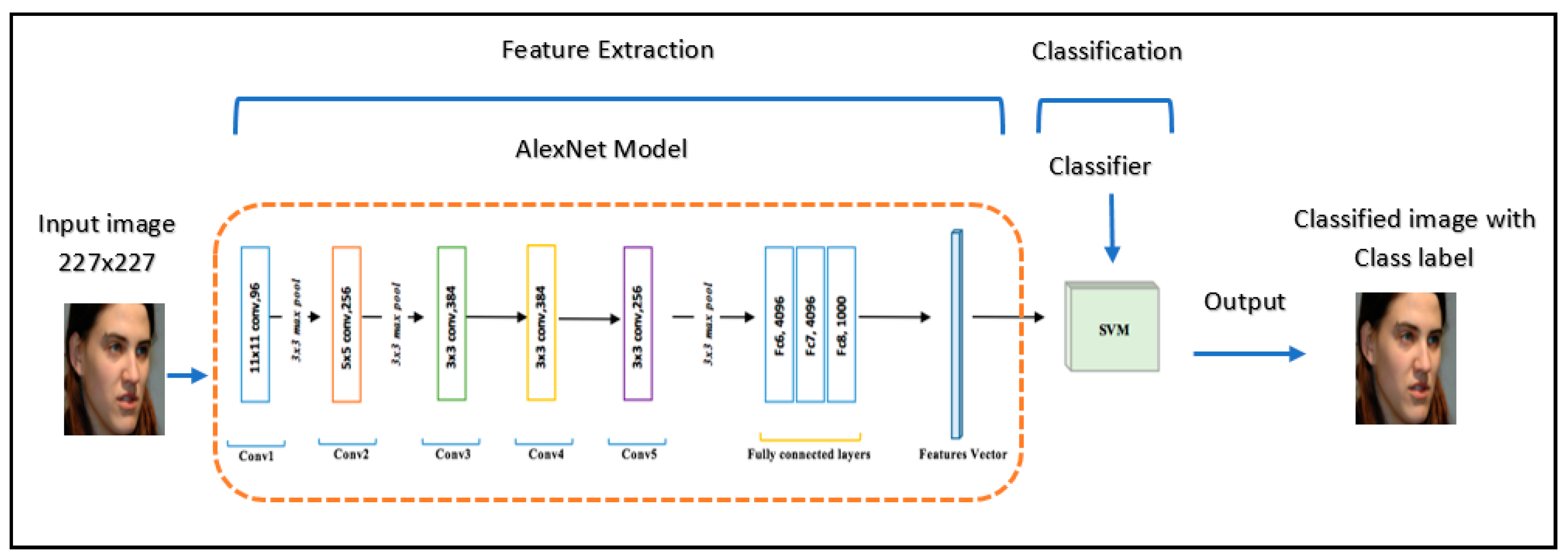
4.2.1. First Experiment: Pre-Trained CNN AlexNet with SVM
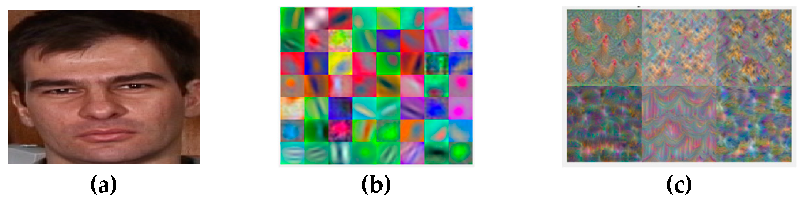
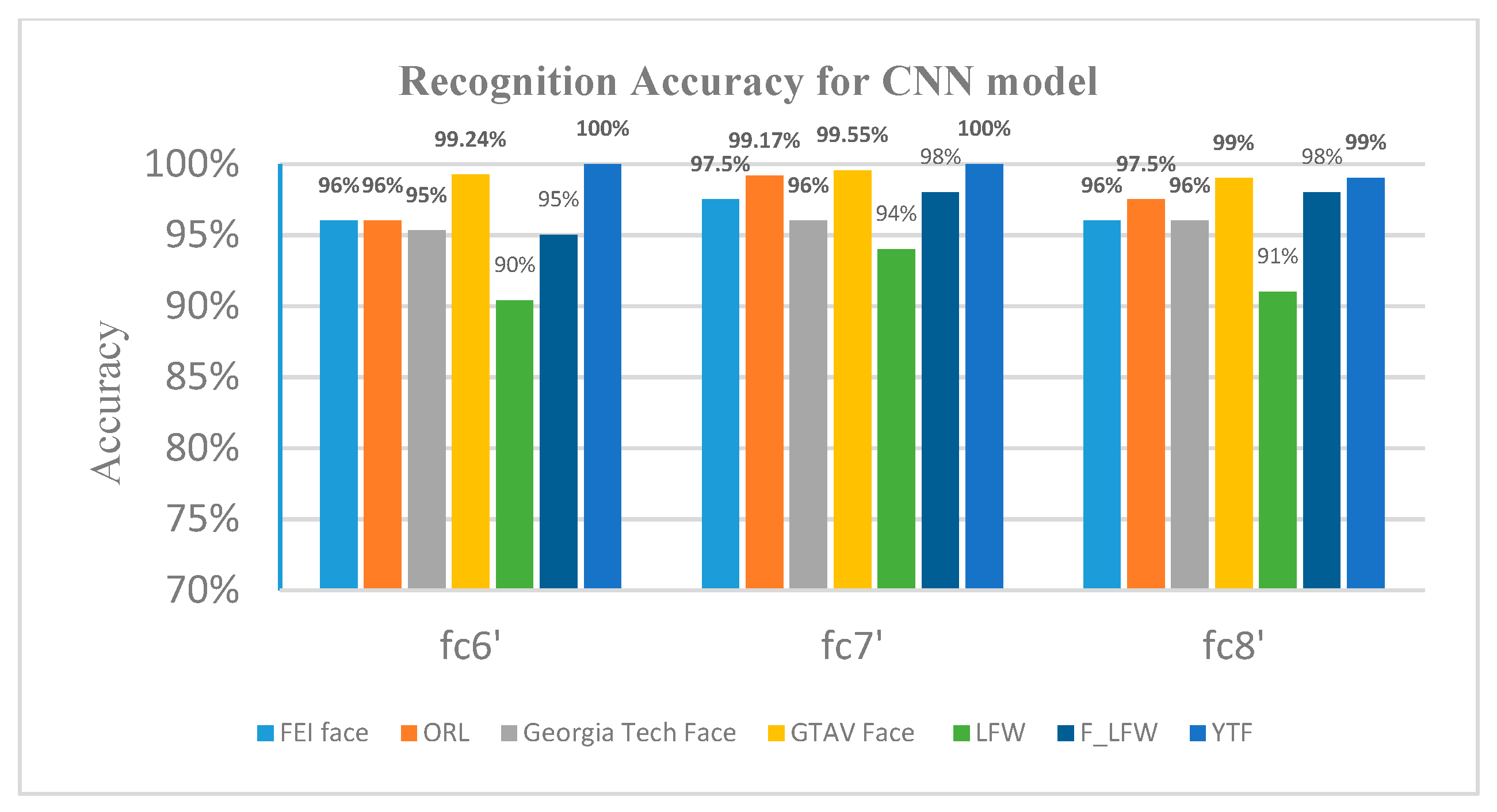
This experiment was conducted by extracting the learned image features from a pre-trained CNN AlexNet, and to train SVM using those features, as shown in Figure 4. As mentioned before, for AlexNet net we needed to resize all images to 227 × 227 and convert any grayscale images to RGB. In our implementation, we split the data into 80% training and 20% test data and randomized the split to avoid biasing the results. AlexNet is made up of numerous layers but it is crucial to note that not all these layers are essential for extracting features. The first layer performs the extraction of features such blobs and edges, as displayed in Figure 5b. Therefore, using deep layers gives better distinct features [56]. Figure 5c shows the extracted features of layer ‘fc7’. In this experiment, we extracted the feature from each layer in a fully-connected layer ‘fc6’, ‘fc7’, ‘fc8’, and compared the performance with different features. Then, we fitted SVM to perform the classification task. The output of feature extraction from ‘fc8’ layer was a 4096-dimensional feature vector. For SVM kernel function, we used linear kernel function without any optimization. The kernel function is used to take vector data as input and transform it into the optimal form. The ’MiniBatchSize’ was set 20. We trained by stochastic gradient descent (SGD). The results of this method were evaluated with all provided datasets. The extracted features from layers ‘fc6’, ‘fc7’, and ‘fc8’ are illustrated in Figure 6. As it can be seen from Figure 6, the features from the ‘fc7’ layer had the highest recognition accuracy. This result clearly confirms that an optimal feature can be extracted from ‘fc7’. The layer ‘fc7’ had additional distinguished power for same-class recognition. As results for this experiment, from Figure 6, we can observe that the network achieved a higher accuracy of 100% on YTF datasets, and 99.55% and 99.17% for the GTAV face and ORL datasets, respectively, whereas for the F_FLW dataset the model obtained 98%. Finally, FEI achieved 97.50%, Georgia Tech face dataset was 96%, and LFW was 94%.
4.2.2. Second Experiment: Pre-Trained ResNet-50 Model with SVM
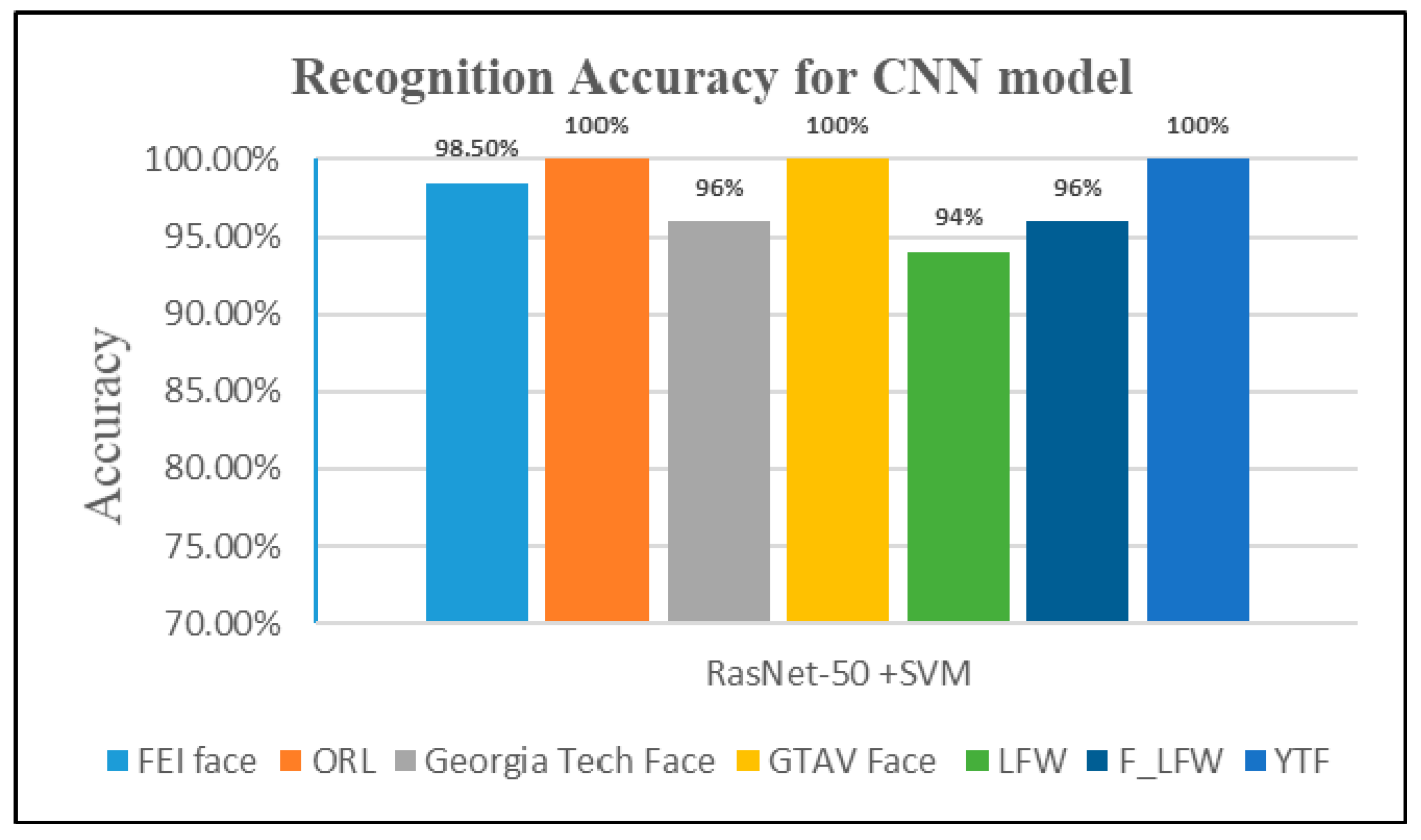
The learned image features from the training images were extracted and followed by SVM classifier, as shown in Figure 7. In the implementation process, we created an Image-Data store to help with data management. This was because, after reading, the images were loaded into the memory system, thus making it effective for a huge collection of images. After uploading, the data were divided into 70% training and 30% validation using random sampling to avoid biasing the results. As a pre-processing stage, ResNet-50 network can only process RGB images that are 224 × 224; here, we resized and convert any grayscale images to RGB. Using deep layers for higher level features gives better distinct features for recognition tasks. For feature extraction, the layer before classification layer, named ‘fc1000’, was used to extract features by using the activation method. These features were then used to train and test SVM classifiers using a fast-linear solver. The activation outputs were arranged into columns to speed-up SVM training that follows, and the fast stochastic gradient descent (SGD) was implemented for the training. The ’MiniBatchSize’ was set 32 to ensure the CNN and image data fitted into the servers’ memory. With regard to results for this experiment, Figure 8 shows that the ResNet-50 model obtained a higher accuracy of 100% on GTAV face, ORL, and YTF datasets. It also obtained 98.50% and 96% recognition accuracy for both FEI and Georgia Tech face datasets, respectively.
4.2.3. Third Experiment: Transfer Learning from AlexNet for Extracting Features and Classification
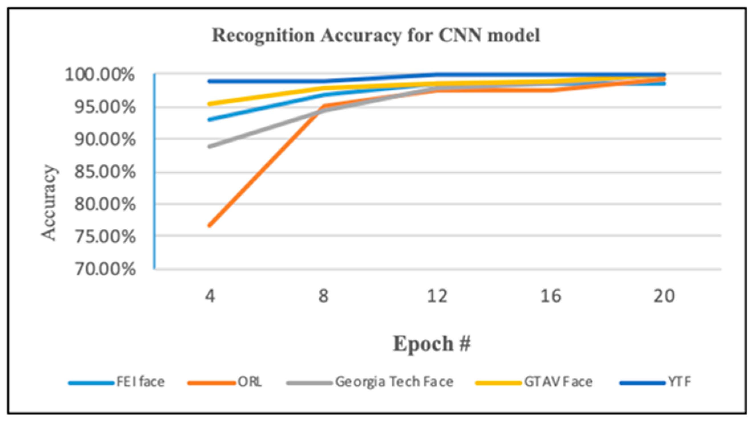
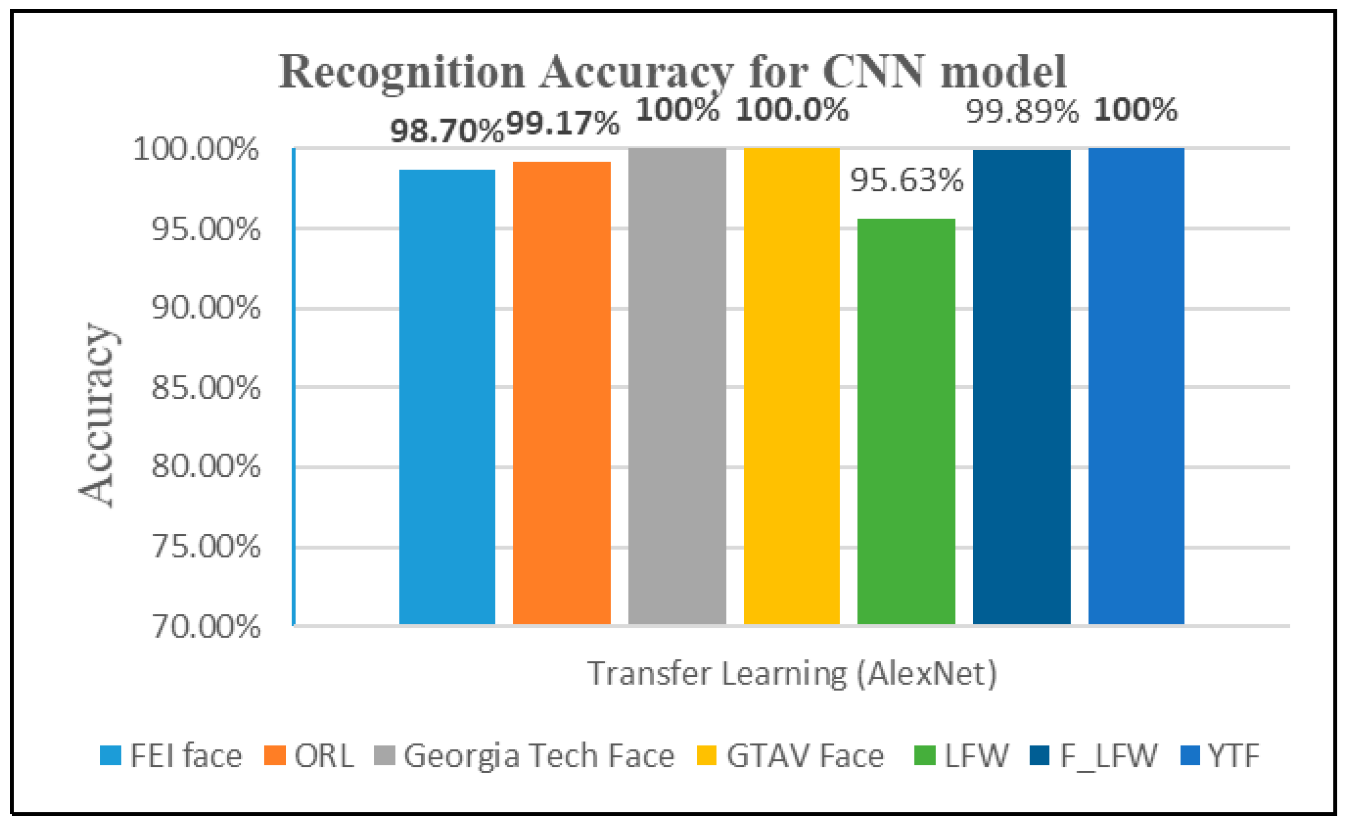
In this experiment, we evaluated the performance when transfer learning from AlexNet network is used for classification task, as shown in Figure 9. AlexNet is a pre-trained net, and it was trained with millions of images for 1000 class problem. It consists of 25 layers; the first 23 layers are for feature extraction, whereas the last 3 layers are for classifying these features into 1000 groups. Thus, in this step, transfer of the layers to the new classification task was done by removing the last three layers and adding the new fully connected layer so that it has a similar size as the number of classes in the new data based on dataset classes. In this experiment, we tested the model with a different number of epochs until it reached a good accuracy, as shown in Figure 10. We found the highest accuracy was obtained with an epoch equal 20. Set the mini-batch size 20. The software validated the network with validation frequency equal to 3 during training. Also, the data was divided into 70% training and 30% validation. As presented in Figure 11, the results of this experiment showed that the highest test accuracy after the training was of 100% on the GTAV face dataset, Georgia Tech face dataset, and YouTube face dataset. Also, the model achieved 99.17% with the ORL dataset, and 98.70% on the FEI face dataset. The network of transfer learning from AlexNet achieved a better performance than AlexNet with the SVM model, as present in Table 5.
4.2.4. Performance Analysis
The performance analysis of all experiments was based on the most common evaluation measures used for statistical tests, such as accuracy, precision, recall, and f_measure. The accuracy was the fraction of the predicted labels that were correct. Accuracy recall was defined as:
where TP is the true positives rate, TN is the true negatives rate, FN is false negatives, and FP is false positives.
Recall represented the fact that the fraction is of true positive instances to the sum of true positives and false negatives. Recall was defined as:
Precision represented fraction of true positive instances to all positive instances. Precision was defined as:
F_Measure represented the combination of precision and recall. F_Measure was defined as:
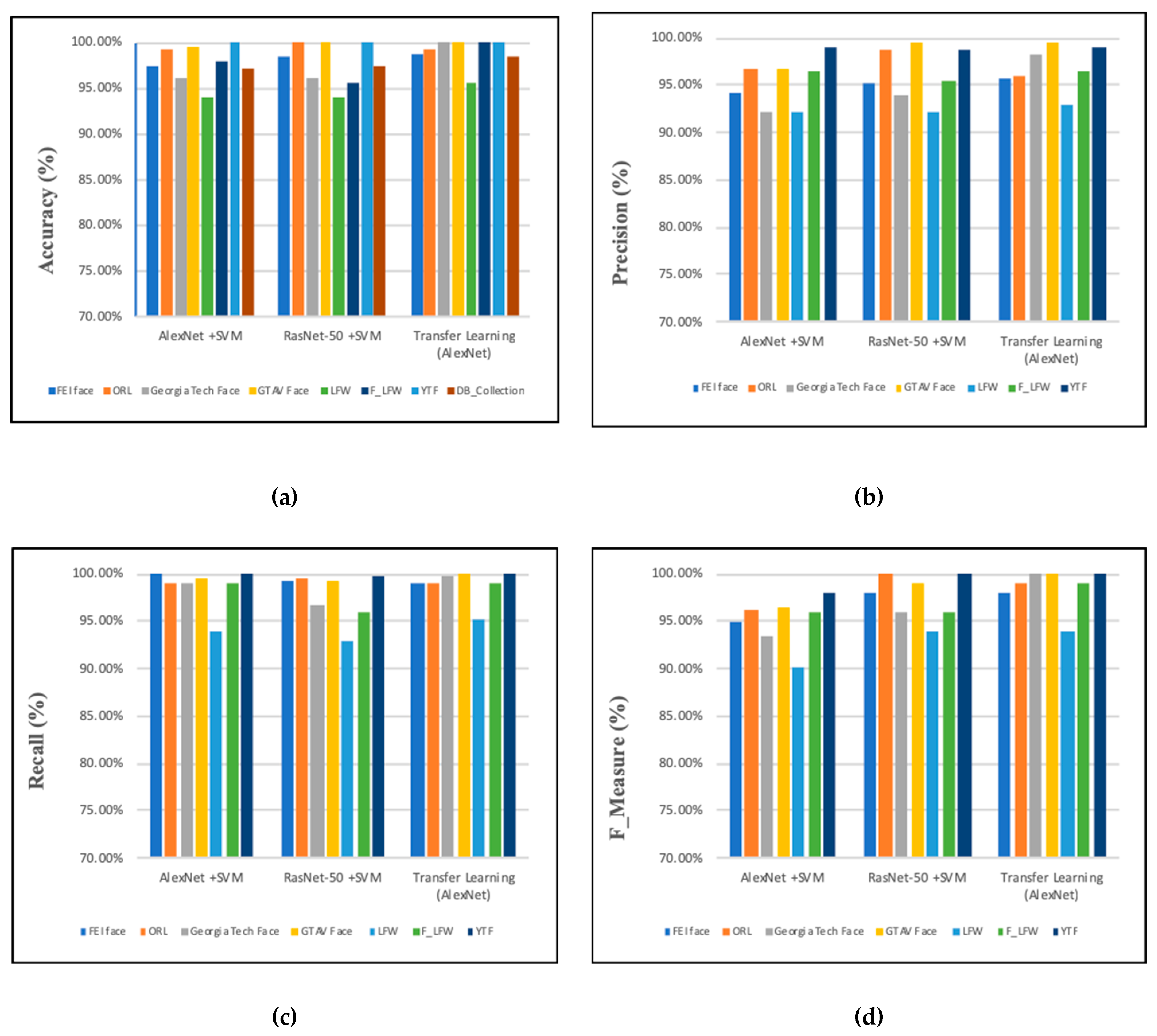
The performance analysis of all the approaches (AlexNet with SVM, ResNet-50 with SVM, and transfer learning from AlexNet) based on accuracy, precision, recall, and F_Measure with all datasets (FEI, ORL, Georgia Tech face, GTAV face, LFW, F_LFW, and YTF) shown in Figure 12. The performance analysis for all models was as follows:
First, in terms of accuracy, as shown in Figure 12a, we can observe that the AlexNet + SVM model obtained the highest results with an accuracy of 100% on the YTF dataset. Also, pre-trained CNN ResNet-50 + SVM achieved an accuracy of 100% on GTAV face dataset, ORL dataset, and YTF dataset. When using transfer learning from the AlexNet model, we can observe the higher accuracy of 100% being achieved on the Georgia Tech face dataset, GTAV face dataset, and YouTube face dataset. Also, we compared the results when testing the models on the DB_Collection dataset that included a combination of images from all datasets. We can observe from Figure 12a the accuracy was 97% with the AlexNet + SVM model, 97.50% with the ResNet-50 + SVM model, and 98.32% with the transfer learning from the AlexNet model.
Second, the results for precision value is illustrated in Figure 12b. The measure value of precision for AlexNet + SVM was in the range of 92%–99% with all datasets. For the approach ResNet-50 + SVM, the values were between 92.22% and 99.50%. Also, transfer learning from AlexNet obtained results between 92.89% and 99.50%. The best results were 99.50% for both ResNet-50 with SVM and transfer learning from AlexNet, and 99.10% with AlexNet + SVM.
Third, Figure 12c presents the results of recall measure for all the approaches (AlexNet with SVM, ResNet-50 with SVM, and transfer learning from AlexNet). All three approaches achieved a high result between 93% and 99.98%.
Finally, Figure 12d shows the performance evaluation in terms of F_Measure. The measure values for all approaches were between 90.1% and 100%. The model transfer learning from AlexNet achieved the highest results with all datasets, but with the ORL dataset, ResNet-50 with SVM obtained the highest value.
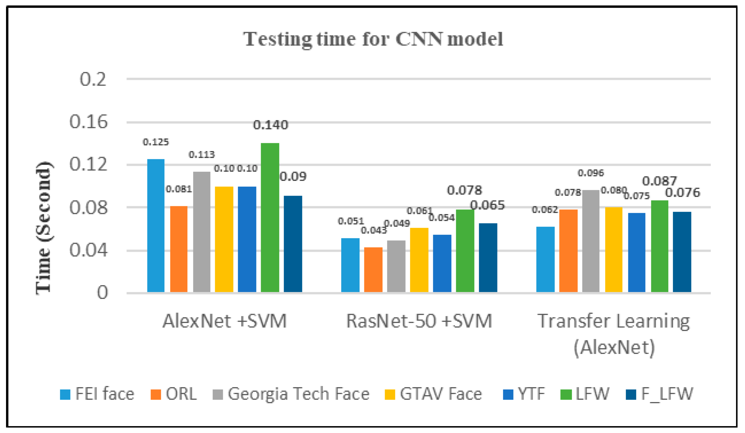
For the testing time, Figure 13 shows ResNet-50 with SVM took less time than other networks with all datasets. The model for transfer learning from pre-trained AlexNet convolutional neural network took less time than AlexNet with SVM with all datasets.
4.3. Comparison with the State-of-the-Art Models
This section presents statistical analysis in the comparison of the performance with the state-of-the-art models in terms of the datasets (FEI face, YouTube face, LFW, and ORL). The statistical analysis was performed on the basis of the accuracy, mean, and variance.
Table 6 shows the performance of our model and the state-of-the-art models, including BQA [39], Hybrid ConvNet-RBM [40], DeepFace [42], CNN-2+ Raw image [43], Deep CNN [49], CNN + SVM [51], DeepFace system [13], DeepID [53], DeepID2 [54], DeepID2+ [55], global expansion ACNN and global + local expansion ACNN [58], and sparse representation face recognition [59].
First, with the FEI faces dataset, the three models achieved a good accuracy—AlexNet with SVM (97.5%), ResNet-50 with SVM (98.5%), and transfer learning on AlexNet (98.7%). The results were higher than sparse representation face recognition [59], and the accuracy was 61.31%.
Second, with the ORL dataset, all three models—AlexNet with SVM, ResNet-50 with SVM, and transfer learning on AlexNet—achieved a higher accuracy than the state-of-the-art models [58] with 91.67% and 93.30%, whereas [51] was 97.5%, and [43] was 95%. We obtained 100% with (ResNet-50 + SVM), 99.17% with (AlexNet + SVM), and transfer learning on AlexNet.
Third, the results of the YouTube face dataset were 100% for all three models—AlexNet with SVM, ResNet-50 with SVM, and transfer learning on AlexNet. The result was higher than [13,39,42,49,55]. We compared our model with DeepID2+ in [55] rather than the previous DeepID model, as DeepID2+ is the latest model of DeepID1 and DeepID2, and gives a final enhancement of the models and high accuracy.
Fourth, with the LFW dataset we conducted our experiments without applying any pre-processing, we simply cropped the face image region to remove the complex background from the images. We obtained 95.63% when using transfer learning from AlexNet and achieved 94% with both AlexNet with SVM and ResNet-50 with SVM. Our results were higher than that of Sun et al. [40]. Also, our models achieved less accuracy than Guo et al. [42], Y. Sun et al. [53], and Y. Sun et al. [54], as we did not apply any pre-processing method and we used the pre-trained model rather than other researchers who built their system from scratch for the FR problem.
Finally, in the time complexity in the comparison, not all models set the illustration for the time. The model ResNet-50 with SVM took less time than other our models.
5. Conclusions
In this paper, pre-trained convolution neural network (CNN) architectures were applied for face biometric system with different approaches. First, we applied the pre-trained CNN AlexNet and ResNet-50 for extracting features and the support vector machine SVM for classification. Second, we applied transfer learning from the AlexNet model for extracting features and classification. In the study, we conducted three experiments. First, we evaluated the performance for pre-trained convolutional neural network AlexNet for extracting learned features and using a multi-class support vector machine (SVM) for the classification task. Second, we evaluated the performance for a pre-trained CNN ResNet-50 for extracting learned features and using an SVM as a classifier. Third, we evaluated the performance for transfer learning from pre-trained CNN AlexNet for the classification task. The investigation study was conducted on various datasets (Georgia Tech face dataset, FEI faces, GTAV face, YouTube face, LFW, F_LFW, ORL, and DB_Collection). The results showed the accuracy range of 94% to 100% for models with all databases obtained. The results for AlexNet with SVM confirmed that an optimal feature can be extracted from ‘fc7’. For the testing time, ResNet-50 with SVM took less time than other networks with all datasets. We compared our model with the state-of-the-art models in terms of the datasets (FEI faces, LFW, YouTube face, and ORL). The results showed that our model achieved a higher accuracy than most of the state-of-the-art models. In the future, we intend to further improve recognition and classification accuracy. To do so, more databases need to be included for training our CNN models, as well as to test different convolutional neural network models for better functioning. An enhancement for FR models can propose new techniques for feature extraction. Moreover, we can investigate the technique to extract features from a different layer and apply cross-validation, as in [60].
Author Contributions
The authors equally contributed to the present paper.
Funding
This research received no external funding.
Conflicts of Interest
There are no known conflicts of interest associated with this publication and there has been no significant financial support for this work that could have influenced its outcome. The manuscript has been read and approved by all named authors and that there are no other persons who satisfied the criteria for authorship but are not listed. We further confirm that the order of authors listed in the manuscript has been approved by all of us.
References
- Purwins, H.; Li, B.; Virtanen, T.; Chang, S.; Sainath, T. Deep Learning for Audio Signal Processing. IEEE J. Sel. Top. Signal Process. 2019, 14, 206–219. [Google Scholar] [CrossRef]
- Bao, Y.; Tang, Z.; Li, H. Computer vision and deep learning–based data anomaly detection method for structural health monitoring. Struct. Health Monit. 2018, 18, 401–421. [Google Scholar] [CrossRef]
- Xue, J.; Han, J.; Zheng, T.; Gao, X.; Guo, J. A Multi-Task Learning Framework for Overcoming the Catastrophic Forgetting in Automatic Speech Recognition. arXiv 2019, arXiv:1904.08039. [Google Scholar]
- Imran, J.; Raman, B. Deep motion templates and extreme learning machine for sign language recognition. Vis. Comput. 2019. [Google Scholar] [CrossRef]
- Ravi, S.; Suman, M.; Kishore, P.V.V.; Kumar, K.; Kumar, A. Multi Modal Spatio Temporal Co-Trained CNNs with Single Modal Testing on RGB–D based Sign Language Gesture Recognition. J. Comput. Lang. 2019, 52, 88–102. [Google Scholar] [CrossRef]
- Al-Emadi, S.; Al-Ali, A.; Mohammad, A.; Al-Ali, A. Audio Based Drone Detection and Identification using Deep Learning. In Proceedings of the 2019 15th International Wireless Communications & Mobile Computing Conference (IWCMC), Tangier, Morocc, 24–28 June 2019; pp. 459–464. [Google Scholar]
- Prasad, P.S.; Pathak, R.; Gunjan, V.K.; Rao, H.V.R. Deep Learning Based Representation for Face Recognition; Springer: Berlin, Germany, 2019; pp. 419–424. [Google Scholar]
- Hu, G.; Yang, Y.; Yi, D.; Kittler, J.; Christmas, W.; Li, S.Z.; Hospedales, T. When face recognition meets with deep learning: An evaluation of convolutional neural networks for face recognition. In Proceedings of the IEEE International Conference on Computer Vision Workshops, Santiago, Chile, 11–12 December 2015; pp. 142–150. [Google Scholar]
- Kshirsagar, V.P.; Baviskar, M.R.; Gaikwad, M.E. Face recognition using Eigenfaces. In Proceedings of the 2011 3rd International Conference on Computer Research and Development, Shanghai, China, 11–13 March 2011; Volume 2, pp. 302–306. [Google Scholar]
- Bartlett, M.S.; Movellan, J.R.; Sejnowski, T.J. Face recognition by independent component analysis. IEEE Trans. Neural Netw. 2002, 13, 1450–1464. [Google Scholar] [CrossRef]
- Ojala, T.; Pietikainen, M.; Maenpaa, T. Multiresolution gray-scale and rotation invariant texture classification with local binary patterns. IEEE Trans. Pattern Anal. Mach. Intell. 2002, 24, 971–987. [Google Scholar] [CrossRef]
- Liu, Y.; Lin, M.; Huang, W.; Liang, J. A physiognomy based method for facial feature extraction and recognition. J. Vis. Lang. Comput. 2017, 43, 103–109. [Google Scholar] [CrossRef]
- Taigman, Y.; Yang, M.; Ranzato, M.; Wolf, L. Deepface: Closing the gap to human-level performance in face verification. In Proceedings of the IEEE Conference on Computer Vision and Pattern Recognition, Columbus, OH, USA, 23–28 June 2014; pp. 1701–1708. [Google Scholar]
- Boufenar, C.; Kerboua, A.; Batouche, M. Investigation on deep learning for off-line handwritten Arabic character recognition. Cogn. Syst. Res. 2018, 50, 180–195. [Google Scholar] [CrossRef]
- Boser, B.E.; Guyon, I.M.; Vapnik, V.N. A training algorithm for optimal margin classifiers. In Proceedings of the Fifth Annual Workshop on Computational Learning Theory, Pittsburgh, PA, USA, 27–29 July 1992; pp. 144–152. [Google Scholar]
- ORL Face Database. Available online: http://www.uk.research.att.com/facedatabase.html (accessed on 6 April 2019).
- Tarres, F.; Rama, A. GTAV Face Database. 2011. Available online: https://gtav.upc.edu/en/research-areas/face-database (accessed on 6 April 2019).
- Nefian, A.V. Georgia Tech Face Database. Available online: http://www.anefian.com/research/face_reco.htm (accessed on 6 April 2019).
- Thomaz, C.E. FEI Face Database. 2012. Available online: https://fei.edu.br/~cet/facedatabase.html (accessed on 6 April 2019).
- Huang, G.B.; Ramesh, M.; Berg, T.; Learned-Miller, E. Labeled Faces in the Wild: A Database for Studying Face Recognition in Unconstrained Environments. 2007. Available online: https://hal.inria.fr/inria-00321923 (accessed on 1 September 2019).
- Frontalized Faces in the Wild. 2016. Available online: https://www.micc.unifi.it/resources/datasets/frontalized-faces-in-the-wild/ (accessed on 6 April 2019).
- Wolf, L.; Hassner, T.; Maoz, I. Face recognition in unconstrained videos with matched background similarity. In Proceedings of the Computer Vision and Pattern Recognition (CVPR), Colorado Springs, CO, USA, 20–25 June 2011; pp. 529–534. [Google Scholar]
- LeCun, Y.; Kavukcuoglu, K.; Farabet, C. Convolutional networks and applications in vision. In Proceedings of the 2010 IEEE International Symposium on Circuits and Systems, Paris, France, 30 May–2 June 2010; pp. 253–256. [Google Scholar]
- LeCun, Y.; Boser, B.E.; Denker, J.S.; Henderson, D.; Howard, R.E.; Hubbard, W.E.; Jackel, L.D. Handwritten digit recognition with a back-propagation network. In Proceedings of the Advances in Neural Information Processing Systems, Denver, CO, USA, 26–29 November 1990; pp. 396–404. [Google Scholar]
- Postorino, M.N.; Sarne, G.M.L. A neural network hybrid recommender system. In Proceedings of the 2011 Conference on Neural Nets WIRN10, Salerno, Italy, 27–29 May 2011; pp. 180–187. [Google Scholar]
- Ciresan, D.C.; Meier, U.; Masci, J.; Gambardella, L.M.; Schmidhuber, J. Flexible, high performance convolutional neural networks for image classification. In Proceedings of the Twenty-Second International Joint Conference on Artificial Intelligence, Catalonia, Spain, 16–22 June 2011; Volume 22, pp. 1237–1242. [Google Scholar]
- Xie, Y.; Le, L.; Zhou, Y.; Raghavan, V.V. Deep Learning for Natural Language Processing. In Handbook of Statistics; Elsevier: Amsterdam, The Netherlands, 2018. [Google Scholar]
- Kumar, R. Natural language processing. In Machine Learning and Cognition in Enterprises; Kumar, R., Ed.; Springer: Berlin, Germany, 2017; pp. 65–73. [Google Scholar]
- Rojas, R. Neural Networks: A Systematic Introduction; Springer: Berlin, Germany, 2013. [Google Scholar]
- Karpathy CS231n Convolutional Neural Networks for Visual Recognition. 2018. Available online: http://cs231n.github.io/convolutional-networks/ (accessed on 8 May 2019).
- Boureau, Y.-L.; Ponce, J.; LeCun, Y. A theoretical analysis of feature pooling in visual recognition. In Proceedings of the 27th International Conference on Machine Learning, Haifa, Israel, 21–24 June 2010; pp. 111–118. [Google Scholar]
- Scherer, D.; Müller, A.; Behnke, S. Evaluation of pooling operations in convolutional architectures for object recognition. In Proceedings of the International Conference on Artificial Neural Networks, Thessaloniki, Greece, 15–18 September 2010; pp. 92–101. [Google Scholar]
- Wu, H.; Gu, X. Max-pooling dropout for regularization of convolutional neural networks. In Proceedings of the International Conference on Neural Information Processing, Istanbul, Turkey, 9–12 November 2015; pp. 46–54. [Google Scholar]
- He, K.; Zhang, X.; Ren, S.; Sun, J. Spatial pyramid pooling in deep convolutional networks for visual recognition. IEEE Trans. Pattern Anal. Mach. Intell. 2015, 37, 1904–1916. [Google Scholar] [CrossRef]
- Ouyang, W.; Wang, X.; Zeng, X.; Qiu, S.; Luo, P.; Tian, Y.; Tang, X. Deepid-net: Deformable deep convolutional neural networks for object detection. In Proceedings of the IEEE Conference on Computer Vision and Pattern Recognition, Boston, MA, USA, 7–12 June 2015; pp. 2403–2412. [Google Scholar]
- Krizhevsky, A.; Sutskever, I.; Hinton, G.E. Imagenet classification with deep convolutional neural networks. In Proceedings of the Advances in Neural Information Processing Systems, Lake Tahoe, CA, USA, 3–6 December 2012; pp. 1097–1105. [Google Scholar]
- Girshick, R.; Donahue, J.; Darrell, T.; Malik, J. Rich feature hierarchies for accurate object detection and semantic segmentation. In Proceedings of the IEEE Conference on Computer Vision and Pattern Recognition, Columbus, OH, USA, 23–28 June 2014; pp. 580–587. [Google Scholar]
- He, K.; Zhang, X.; Ren, S.; Sun, J. Deep Residual Learning for Image Recognition. In Proceedings of the IEEE Conference on Computer Vision and Pattern Recognition, Las Vegas, NV, USA, 27–30 June 2016; pp. 770–778. [Google Scholar]
- Yu, J.; Sun, K.; Gao, F.; Zhu, S. Face biometric quality assessment via light CNN. Pattern Recognit. Lett. 2018, 107, 25–32. [Google Scholar] [CrossRef]
- Sun, Y.; Wang, X.; Tang, X. Hybrid deep learning for computing face similarities. Int. Conf. Comput. Vis. 2013, 38, 1997–2009. [Google Scholar]
- Singh, R.; Om, H. Newborn face recognition using deep convolutional neural network. Multimed. Tools Appl. 2017, 76, 19005–19015. [Google Scholar] [CrossRef]
- Guo, K.; Wu, S.; Xu, Y. Face recognition using both visible light image and near-infrared image and a deep network. CAAI Trans. Intell. Technol. 2017, 2, 39–47. [Google Scholar] [CrossRef]
- Hu, H.; Afaq, S.; Shah, A.; Bennamoun, M.; Molton, M. 2D and 3D Face Recognition Using Convolutional Neural Network. In Proceedings of the TENCON 2017 IEEE Region 10 Conference, Penang, Malaysia, 5–8 November 2017; pp. 133–138. [Google Scholar]
- Nam, G.P.; Choi, H.; Cho, J. PSI-CNN: A Pyramid-Based Scale-Invariant CNN Architecture for Face Recognition Robust to Various Image Resolutions. Appl. Sci. 2018, 8, 1561. [Google Scholar] [CrossRef]
- Khan, S.; Javed, M.H.; Ahmed, E.; Shah, S.A.A.; Ali, S.U. Networks and Implementation on Smart Glasses. In Proceedings of the 2019 International Conference on Information Science and Communication Technology (ICISCT), Karachi, Pakistan, 9–10 March 2019; pp. 1–6. [Google Scholar]
- Qin, C.; Lu, X.; Zhang, P.; Xie, H.; Zeng, W. Identity Recognition Based on Face Image. J. Phys. Conf. Ser. 2019, 1302, 032049. [Google Scholar] [CrossRef]
- Menotti, D.; Chiachia, G.; Pinto, A.; Schwartz, W.R.; Pedrini, H.; Falcao, A.X.; Rocha, A. Deep Representations for Iris, Face, and Fingerprint Spoofing Detection. IEEE Trans. Inf. Forensics Secur. 2015, 10, 864–879. [Google Scholar] [CrossRef] [Green Version]
- Simón, M.O.; Corneanu, C.; Nasrollahi, K.; Nikisins, O.; Escalera, S.; Sun, Y.; Greitans, M. Improved RGB-D-T based face recognition. IET Biom. 2016, 5, 297–303. [Google Scholar] [CrossRef]
- Parkhi, O.M.; Vedaldi, A.; Zisserman, A. Deep Face Recognition. BMVC 2015, 1, 6. [Google Scholar]
- Zhu, Z.; Luo, P.; Wang, X.; Tang, X. Recover canonical-view faces in the wild with deep neural networks. arXiv 2014, arXiv:1404.3543. [Google Scholar]
- Guo, S.; Chen, S.; Li, Y. Face recognition based on convolutional neural network & support vector machine. In Proceedings of the 2016 IEEE International Conference on Information and Automation (ICIA), Ningbo, China, 1–3 August 2016; pp. 1787–1792. [Google Scholar]
- Lawrence, S.; Giles, C.L.; Tsoi, A.C.; Back, A.D. Face recognition: A convolutional neural-network approach. IEEE Trans. Neural Netw. 1997, 8, 98–113. [Google Scholar] [CrossRef] [PubMed]
- Sun, Y.; Wang, X.; Tang, X. Deep Learning Face Representation from Predicting 10,000 Classes. In Proceedings of the IEEE Conference on Computer Vision and Pattern Recognition, Columbus, OH, USA, 23–28 June 2014; pp. 1891–1898. [Google Scholar]
- Sun, Y.; Chen, Y.; Wang, X.; Tang, X. Deep Learning Face Representation by Joint Identification-Verification. In Proceedings of the Advances in Neural Information Processing Systems 27, Montreal, QC, Canada, 8–13 December 2014; pp. 1988–1996. [Google Scholar]
- Sun, Y.; Wang, X.; Tang, X. Deeply Learned Face Representations Are Sparse, Selective, and Robust. In Proceedings of the IEEE Conference on Computer Vision and Pattern Recognition, Boston, MA, USA, 7–12 June 2015; pp. 2892–2900. [Google Scholar]
- Lu, Z.; Jiang, X.; Kot, A.C. Deep Coupled ResNet for Low-Resolution Face Recognition. IEEE Signal Process. Lett. 2018, 25, 526–530. [Google Scholar] [CrossRef]
- Ferrari, C.; Lisanti, G.; Berretti, S.; del Bimbo, A. Effective 3D based frontalization for unconstrained face recognition. In Proceedings of the 2016 23rd International Conference on Pattern Recognition (ICPR), Cancun, Mexico, 4–8 December 2016; pp. 1047–1052. [Google Scholar]
- Zhang, Y.; Zhao, D.; Sun, J.; Zou, G.; Li, W. Adaptive Convolutional Neural Network and Its Application in Face Recognition. Neural Process. Lett. 2016, 43, 389–399. [Google Scholar] [CrossRef]
- Cai, J.; Chen, J.; Liang, X. Single-sample face recognition based on intra-class differences in a variation model. Sensors 2015, 15, 1071–1087. [Google Scholar] [CrossRef]
- Chui, K.; Lytras, M.D. A Novel MOGA-SVM Multinomial Classification for Organ Inflammation Detection. Appl. Sci. 2019, 9, 2284. [Google Scholar] [CrossRef]
Figure 1.
A typical convolutional network architecture [23].
Figure 1.
A typical convolutional network architecture [23].

Figure 2.
An overview of system approaches.

Figure 3.
Sample images from all datasets: (a) sample images from ORL dataset; (b) sample images from GTAV face dataset; (c) sample images from Georgia Tech face dataset; (d) sample images from FEI dataset; (e) sample images from LFW dataset; (f) sample images from F_LFW dataset; (g) sample images from YTF dataset.

Figure 4.
AlexNet convolutional neural networks with SVM.

Figure 5.
Feature visualization for CNN AlexNet on Georgia Tech face dataset: (a) input image; (b) features of first convolutional layer ’conv1’; (c) features of layer ‘fc7’.
Figure 5.
Feature visualization for CNN AlexNet on Georgia Tech face dataset: (a) input image; (b) features of first convolutional layer ’conv1’; (c) features of layer ‘fc7’.

Figure 6.
Recognition accuracy for AlexNet with features from layers ‘fc6’, ‘fc7’, and ‘fc8’.

Figure 7.
ResNet-50 convolutional neural networks with SVM.

Figure 8.
Recognition accuracy for ResNet-50 with SVM.

Figure 9.
Transfer learning from AlexNet convolutional neural networks.

Figure 10.
Accuracy for CNN models.

Figure 11.
Recognition accuracy for transfer learning from AlexNet model.

Figure 12.
Performance analysis for approaches with all datasets: (a) Accuracy, (b) Precision, (c) Recall, (d) F_Measure.
Figure 12.
Performance analysis for approaches with all datasets: (a) Accuracy, (b) Precision, (c) Recall, (d) F_Measure.

Figure 13.
Testing time for convolutional neural network models.


Table 1.
Details of AlexNet layers.
| Layer | Number of Kernels | Kernel Size | Stride | Padding | Output Size |
|---|---|---|---|---|---|
| Input | [227 × 227 × 3] | ||||
| Conv1 | 96 | 11 × 11 × 3 | 4 | - | [55 × 55 × 96] |
| Max pool1 | 3 × 3 | 2 | - | [27 × 27 × 96] | |
| Norm1 | [27 × 27 × 96] | ||||
| Conv2 | 256 | 5 × 5 × 48 | 1 | 2 | [27 × 27 × 256] |
| Maxpool2 | 3 × 3 | 2 | - | [13 × 13 × 256] | |
| Norm 2 | [13 × 13 × 256] | ||||
| Conv3 | 384 | 3 × 3 × 256 | 1 | 1 | [13 × 13 × 384] |
| Conv4 | 384 | 3 × 3 × 192 | 1 | 1 | [13 × 13 × 384] |
| Conv5 | 256 | 3 × 3 × 192 | 1 | 1 | [13 × 13 × 256] |
| Max pool3 | 3 × 3 | 2 | - | [6 × 6 × 256] | |
| fc6 ReLU Dropout(0.5) | 1 | 4096 | |||
| fc 7 ReLU Dropout(0.5) | 1 | 4096 | |||
| fc8 softmax | 1 | 1000 |
Table 2.
Details of ResNet-50 layers.
| Layer | Kernel Size | Stride | Padding | Output Size |
|---|---|---|---|---|
| Input | [224 × 224 × 3] | |||
| Conv1 | 7 × 7 × 3 | 2 | 3 | [112 × 112 × 64] |
| Max pool | 3 × 3 | 2 | - | [56 × 56] |
| Conv2 | [1×1conv,64],[3 × 3conv,64],1 × 1conv,256] | 2 | - | [56 × 56] |
| [1×1conv,64],[3 × 3conv,64],1 × 1conv,256] | 1 | - | ||
| [1×1conv,64],[3 × 3conv,64],1 × 1conv,256] | 1 | - | ||
| Conv3 | [1×1conv,128],[3 × 3conv,128],[1 × 1conv,512] | 2 | - | [28 × 28] |
| [1×1conv,128],[3 × 3conv,128],[1 × 1conv,512] | 1 | - | ||
| [1×1conv,128],[3 × 3conv,128],[1 × 1conv,512] | 1 | - | ||
| [1×1conv,128],[3 × 3conv,128],[1 × 1conv,512] | 1 | - | ||
| Conv4 | [1×1conv,256],[3 × 3conv,256],[1 × 1conv,1024] | 2 | - | [14 × 14] |
| [1×1conv,256],[3 × 3conv,256],[1 × 1conv,1024] | 1 | - | ||
| [1×1conv,256],[3 × 3conv,256],[1 × 1conv,1024] | 1 | - | ||
| [1×1conv,256],[3 × 3conv,256],[1 × 1conv,1024] | 1 | - | ||
| [1×1conv,256],[3 × 3conv,256],[1 × 1conv,1024] | 1 | - | ||
| [1×1conv,256],[3 × 3conv,256],[1 × 1conv,1024] | 1 | - | ||
| Conv5 | [1×1conv,512],[3 × 3conv,512],[1 × 1conv,2048] | 2 | - | [7 × 7] |
| [1×1conv,512],[3 × 3conv,512],[1 × 1conv,2048] | 1 | - | ||
| [1×1conv,512],[3 × 3conv,512],[1 × 1conv,2048] | 1 | - | ||
| Average pool | 7 × 7 | 7 | - | [1 × 1] |
| fc1000 softmax | 1000 |
Table 3.
Summary of the related work.
| References | Convolutional Neural Network (CNN) Model | Dataset | Accuracy |
|---|---|---|---|
| Yu et al. (2017) [39] | A novel biometric quality assessment (BQA) method based on light CNN | CASIA, FLW, and YouTube | 99.01% |
| Sun et al. (2016) [40] | Hybrid ConvNet-restricted Boltzmann machine (RBM) | Labeled faces in the wild (LFW), CelebFaces | 97.08% (CelebFaces) 93.83% (LFW) |
| Singh and Om (2017) [41] | DeepCNN | IIT(BHU) newborn database | 91.03% |
| Guo et al. (2017) [42] | DeepFace based on DNN used VGGNet | LFW, YouTube face (YTF) | 97.35% |
| Hu et al. (2017) [43] | CNN-2 model | ORL | 95% |
| G. P. Nam et al. (2018) [44] | PSI-CNN | LFW, CCTV | 98.87% |
| P. S. Prasad et al. (2019) [7] | Deep learning based | AR | - |
| Suleman Khan et al. (2019) [45] | Deep CNN | - | 98.5% |
| Chen Qin et al. (2019) [46] | Deep CNN | - | 94.67% |
| Menotti et al. (2015) [47] | Hyperopt-convnet for architecture optimization (AO) based on CNN Cuda-convnet for filter optimization (FO) based on back-propagation algorithm | Replay-Attack, 3DMAD | |
| Simón et al.(2016) [48] | CNN-based | RGB-D-T | |
| O. M. Parkhi et al. (2015) [49] | Deep CNN | LFW, YTF | 98.95% |
| Z. Zhu et al. (2014) [50] | Facial component-based network | LFW, CelebFaces | 96.45 |
| Guo et al. (2017) [51] | CNN + support vector machine (SVM) | ORL | 97.50% |
| Y. Taigman et al. (2014) [13] | DeepFace system | SFC , LFW, YTF | 97.35% |
| Y. Sun et al. (2014) [53] | DeepID | LFW | 97.45% |
| Y. Sun et al. (2014) [54] | DeepID2 | LFW | 99.15% |
| Y. Sun et al. (2015) [55] | DeepID2+ | LFW, YTF | 99.47% (LFW) 93.2% (YTF) |
| Lu et al. (2018) [56] | Deep coupled ResNet (DCR) | LFW, SCface | 99% |
Table 4.
Face datasets and their specifications used in our experiments.
| Datasets | Identities | Images | Images Per Identities | Images Size | Images Type |
|---|---|---|---|---|---|
| ORL | 40 | 400 | 10 | 92 × 112 | JPEG |
| GTAV face | 44 | 704 | 16 | 240 × 320 | BMP |
| Georgia Tech face | 50 | 700 | 14 | 131 × 206 | JPEG |
| FEI face | 50 | 700 | 14 | 640 × 480 | JPEG |
| Labeled faces in the wild (LFW) | 50 | 700 | 14 | 250 × 250 | JPEG |
| Frontalized labeled faces in the wild (F_LFW) | 50 | 700 | 14 | 272 × 323 | JPEG |
| YouTube face (YTF) | 50 | 700 | 14 | 320 × 240 | JPEG |
| DB_Collection | 210 | 2880 | 10-16 | - | - |
Table 5.
Comparison of results with AlexNet with SVM and transfer learning on AlexNet.
| FEI Face | ORL | Georgia Tech Face | GTAV Face | LFW | F_LFW | YTF | |
|---|---|---|---|---|---|---|---|
| AlexNet + SVM | 97.50% | 99.17% | 96% | 99.55% | 94% | 98% | 100% |
| Transfer learning (AlexNet) | 98.70% | 99.17% | 100% | 100% | 95.63% | 99.3% | 100% |
Table 6.
Comparison of results with other face recognition (FR) models.
| References | Model | Datasets | Recognition Accuracy | Mean | Variance | Time |
|---|---|---|---|---|---|---|
| Sun et al. (2016) [40] | Hybrid ConvNet-RBM | LFW | 93.83% | 93.80 | 0.03 | Not available |
| Guo et al. (2017) [42] | DeepFace based on DNN using VGGNet | LWF | 97.35% | 97.32 | 0.03 | Not available |
| Y. Sun et al. (2014) [53] | DeepID | LFW | 97.45% | 97.33 | 0.02 | Not available |
| Y. Sun et al. (2014) [54] | DeepID2 | LFW | 99.15% | 99.12 | 0.03 | Not available |
| Yu et al. (2017) [39] | BQA method based on CNN | YTF | 99.01% | 99.00 | 0.01 | Not available |
| Guo et al. (2017) [42] | DeepFace based on DNN using VGGNet | YTF | 97.35% | 97.32 | 0.03 | Not available |
| O. M. Parkhi et al. (2015) [49] | Deep CNN | YTF | 98.95% | 98.92 | 0.03 | Not available |
| Y. Taigman et al. (2014) [13] | DeepFace system | YTF | 97.35% | 97.32 | 0.03 | Not available |
| Y. Sun et al. (2015) [55] | DeepID2+ | YTF | 93.20% | 93.17 | 0.03 | Not available |
| Y. Zhang (2015) [58] | Global expansion ACNN | ORL | 91.67% | 91.65 | 0.02 | 4.58 min |
| Y. Zhang (2015) [58] | Global + local Expansion ACNN | ORL | 93.30% | 93.27 | 0.03 | 5.7 min |
| S. Guo et al. (2017) [51] | CNN + SVM | ORL | 97.50% | 97.47 | 0.03 | 0.46 min |
| H. Hu et al. (2017) [43] | CNN-2 | ORL | 95.00% | 94.97 | 0.03 | Not available |
| J. Cai et al. (2015) [59] | Sparse representation face recognition | FEI face | 61.31% | 61.30 | 0.01 | Not available |
| Our proposed model (2019) | AlexNet + SVM | FEI face | 97.50% | 97.47 | 0.03 | 0.125 s |
| RasNet-50 + SVM | 98.50% | 98.47 | 0.03 | 0.051 s | ||
| Transfer learning (AlexNet) | 98.70% | 98.67 | 0.03 | 0.062 s | ||
| AlexNet + SVM | ORL | 99.17% | 99.15 | 0.02 | 0.081 s | |
| RasNet-50 + SVM | 100% | 100 | 0 | 0.043 s | ||
| Transfer learning (AlexNet) | 99.17% | 99.15 | 0.02 | 0.078 s | ||
| AlexNet + SVM | YTF | 100% | 100 | 0 | 0.10 s | |
| RasNet-50 + SVM | 100% | 100 | 0 | 0.054 s | ||
| Transfer learning (AlexNet) | 100% | 100 | 0 | 0.075 s | ||
| AlexNet + SVM | LFW | 94% | 93.97 | 0.03 | 0.140 s | |
| RasNet-50 + SVM | 94% | 93.97 | 0.03 | 0.078 s | ||
| Transfer learning (AlexNet) | 95.63% | 95.60 | 0.03 | 0.087 s |
© 2019 by the authors. Licensee MDPI, Basel, Switzerland. This article is an open access article distributed under the terms and conditions of the Creative Commons Attribution (CC BY) license (http://creativecommons.org/licenses/by/4.0/).
Share and Cite
MDPI and ACS Style
Almabdy, S.; Elrefaei, L. Deep Convolutional Neural Network-Based Approaches for Face Recognition. Appl. Sci. 2019, 9, 4397. https://0-doi-org.brum.beds.ac.uk/10.3390/app9204397
AMA Style
Almabdy S, Elrefaei L. Deep Convolutional Neural Network-Based Approaches for Face Recognition. Applied Sciences. 2019; 9(20):4397. https://0-doi-org.brum.beds.ac.uk/10.3390/app9204397
Chicago/Turabian StyleAlmabdy, Soad, and Lamiaa Elrefaei. 2019. "Deep Convolutional Neural Network-Based Approaches for Face Recognition" Applied Sciences 9, no. 20: 4397. https://0-doi-org.brum.beds.ac.uk/10.3390/app9204397
Note that from the first issue of 2016, this journal uses article numbers instead of page numbers. See further details here.