Multilayer Perceptron-Based Phenological and Radiometric Normalization for High-Resolution Satellite Imagery


1
Department of Advanced Technology Fusion, Konkuk University, Seoul 05029, Korea
2
Department of Technology Fusion Engineering, Konkuk University, Seoul 05029, Korea
*
Author to whom correspondence should be addressed.
Appl. Sci. 2019, 9(21), 4543; https://0-doi-org.brum.beds.ac.uk/10.3390/app9214543
Submission received: 12 August 2019
/
Revised: 18 September 2019
/
Accepted: 24 October 2019
/
Published: 25 October 2019
(This article belongs to the Special Issue Machine Learning Techniques Applied to Geospatial Big Data)
Abstract
:Radiometric normalization is an essential preprocessing step that must be performed to detect changes in multi-temporal satellite images and, in general, relative radiometric normalization is utilized. However, most relative radiometric normalization methods assume a linear relationship and they cannot take into account nonlinear properties, such as the distribution of the earth’s surface or phenological differences that are caused by the growth of vegetation. Thus, this paper proposes a novel method that assumes a nonlinear relationship and it uses a representative nonlinear regression model—multilayer perceptron (MLP). The proposed method performs radiometric resolution compression while considering both the complexity and time cost, and radiometric control set samples are extracted based on a no-change set method. Subsequently, the spectral index is selected for each band to compensate for the phenological properties, phenological normalization is performed based on MLP, and the global radiometric properties are adjusted through postprocessing. Finally, a performance evaluation is conducted by comparing the results herein with those from conventional relative radiometric normalization algorithms. The experimental results show that the proposed method outperforms conventional methods in terms of both visual inspection and quantitative evaluation. In other words, the applicability of the proposed method to the normalization of multi-temporal images with nonlinear properties is confirmed.
1. Introduction
With the development of various high-resolution satellite sensors, it is possible to precisely monitor the surface of the earth [1]. In particular, multi-temporal satellite images are an effective data source that can detect changes in land use and land cover [2,3]; however, it is difficult to maintain radiometric consistency in multi-temporal images due to changes in atmospheric conditions, sensor-target-illumination geometry, sensor calibration, and differences in phenological conditions [4,5]. Therefore, radiometric normalization, which is a preprocessing procedure, is performed to reduce—or eliminate—radiometric differences due to the aforementioned influences and increase sensitivity to landscape changes [6,7].
Radiometric normalization can be divided into two main categories: (1) absolute radiometric normalization and (2) relative radiometric normalization [7,8]. Absolute radiometric normalization aims to convert digital numbers (DNs) that are recorded by satellite sensors to ground surface reflectance and corrects factors, such as sensor differences, solar angles, and atmospheric effects [9]. In other words, accurate sensor calibration parameters and atmospheric properties at the time of data acquisition are required. However, it is often difficult to collect such data in terms of cost or accessibility, and the process cannot be implemented when data are not available [10,11,12]. Relative radiometric normalization, on the other hand, is an image-based normalization method that selects one image as a reference and matches the radiometric characteristics of a subject image [13,14]. That is, relative radiometric normalization is generally utilized since the multi-temporal images are normalized into common scales without extra parameters [12,15].
Relative radiometric normalization can be classified into two categories: a global statistics-based method and a radiometric control set sample (RCSS)-based method. The former is performed by using statistical values of all pixels in the image, which includes histogram matching, minimum-maximum (MM), mean-standard deviation (MS), and simple regression (SR) [15,16]. In contrast, the latter is based on invariant pixels, known as RCSSs, which include dark set–bright set (DB), pseudo invariant features (PIF), and no-change sets (NC) [17,18,19,20]. At this time, except for histogram matching, normalization is performed through regression equations, while assuming a linear relationship between the pixels at the same position in each band [21]. However, most remote sensing data are nonlinearly distributed, and the surface of the earth is composed of a complex mixture of natural and man-made features that exhibit nonlinear characteristics [22,23,24]. Changes that are caused by vegetation in particular have the most typical characteristics, including nonlinearity, which induces serious disturbances when change detection is performed [25,26]. In addition, since optical satellite imagery, which is the main source in change detection, is affected by clouds and atmospheric conditions, it is difficult to acquire images that meet the temporal requirements [27,28]. In such cases, images with phenological differences as well as radiometric differences should be utilized [25,26]. In other words, compositive normalizations, including phenological and radiometric properties, should be conducted.
This study proposes a nonlinear relative radiometric normalization method while considering the phenological as well as radiometric properties for high-resolution satellite images in order to overcome these limitations. Among all of the nonlinear regression models, the proposed method is based on multilayer perceptron (MLP), which has advantages over statistical methods, such as a lack of assumptions regarding the probabilistic models of data, robustness to noise, and the ability to learn complex and nonlinear patterns [29,30]. In particular, MLP has been verified as an excellent neural network algorithm at the pixel-level in remote sensing applications, such as cloud masking, image classification, water extraction, or change detection [31,32,33,34]. However, the application of MLP to radiometric and phenological normalizations of high-resolution satellite images is relatively rare. That is, based on these motivations, the proposed method establishes a relationship through MLP to perform relative radiometric normalization. The experiments are conducted on multiple scenes to demonstrate the ability and performance of MLP. Afterwards, the proposed method is comprehensively compared with conventional linear relationship-based methods and nonlinear relationship-based methods. Furthermore, an additional dataset is constructed and applied to the proposed method to verify the robustness of the approach. The rest of this paper is structured, as follows. Section 2 describes the images that were used in this study and the proposed algorithm, including MLP. In Section 3, the results of the proposed method are presented, and detailed comparisons with conventional relative radiometric normalization algorithms and additional discussions are made. Section 4 then concludes this paper.
2. Materials and Methods
2.1. Study Site and Dataset
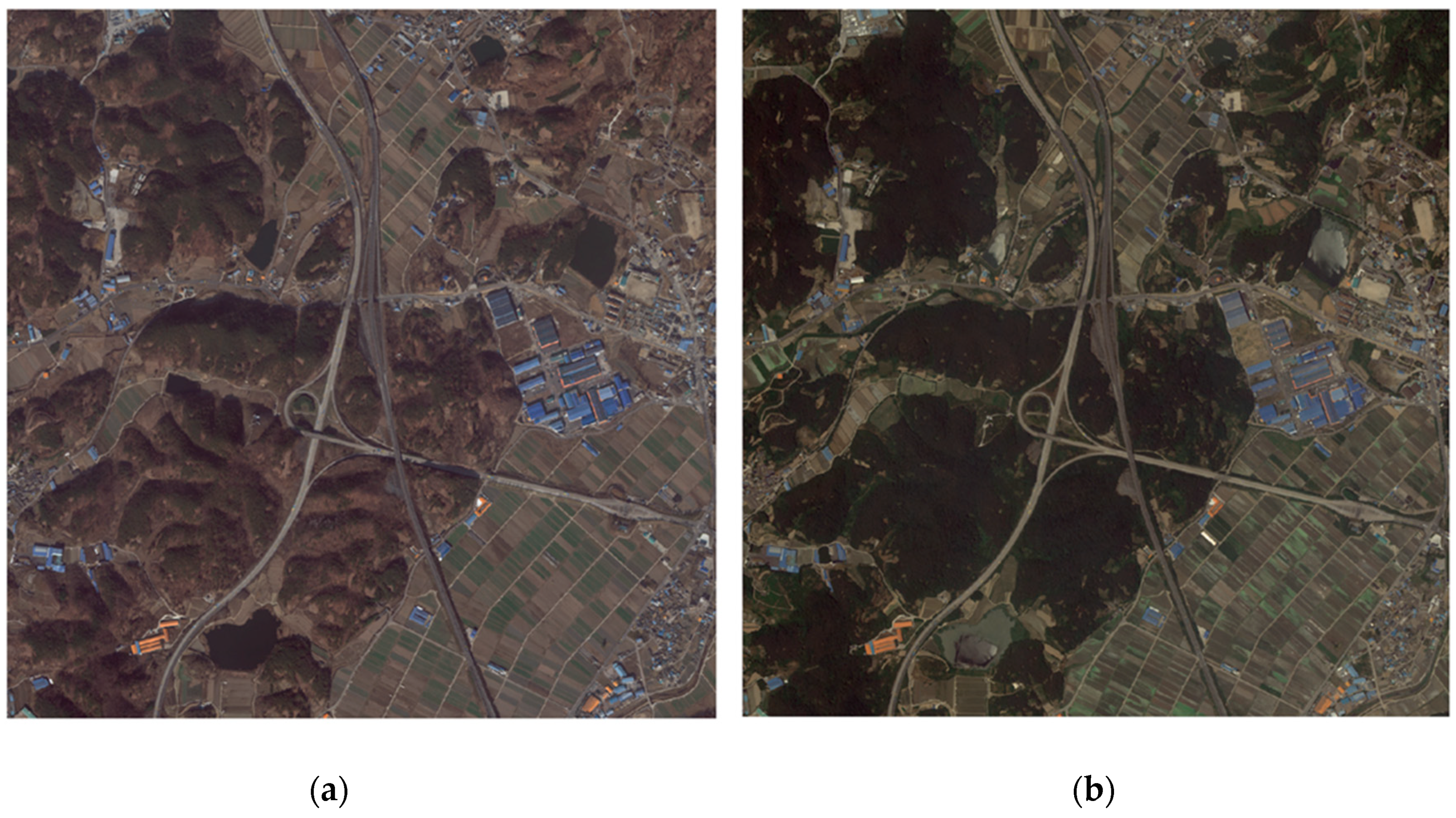
The study site is located in Changnyeong-gun (~128°21′–128°39′ E, ~35°22′–35°44′ N), which is located in the southeastern part of South Korea and is covered by forests, crops, barren lands, water, and built-up areas. This area is mainly composed of vegetation, forests, grasses, and crops, where the spectral characteristics of the forests vary with the season and the spectral characteristics of grasses and crops are heterogeneous, as the state continuously changes. In other words, since it is sensitive to phenological characteristics, it is considered to be suitable for identifying radiometric and phenological effects.
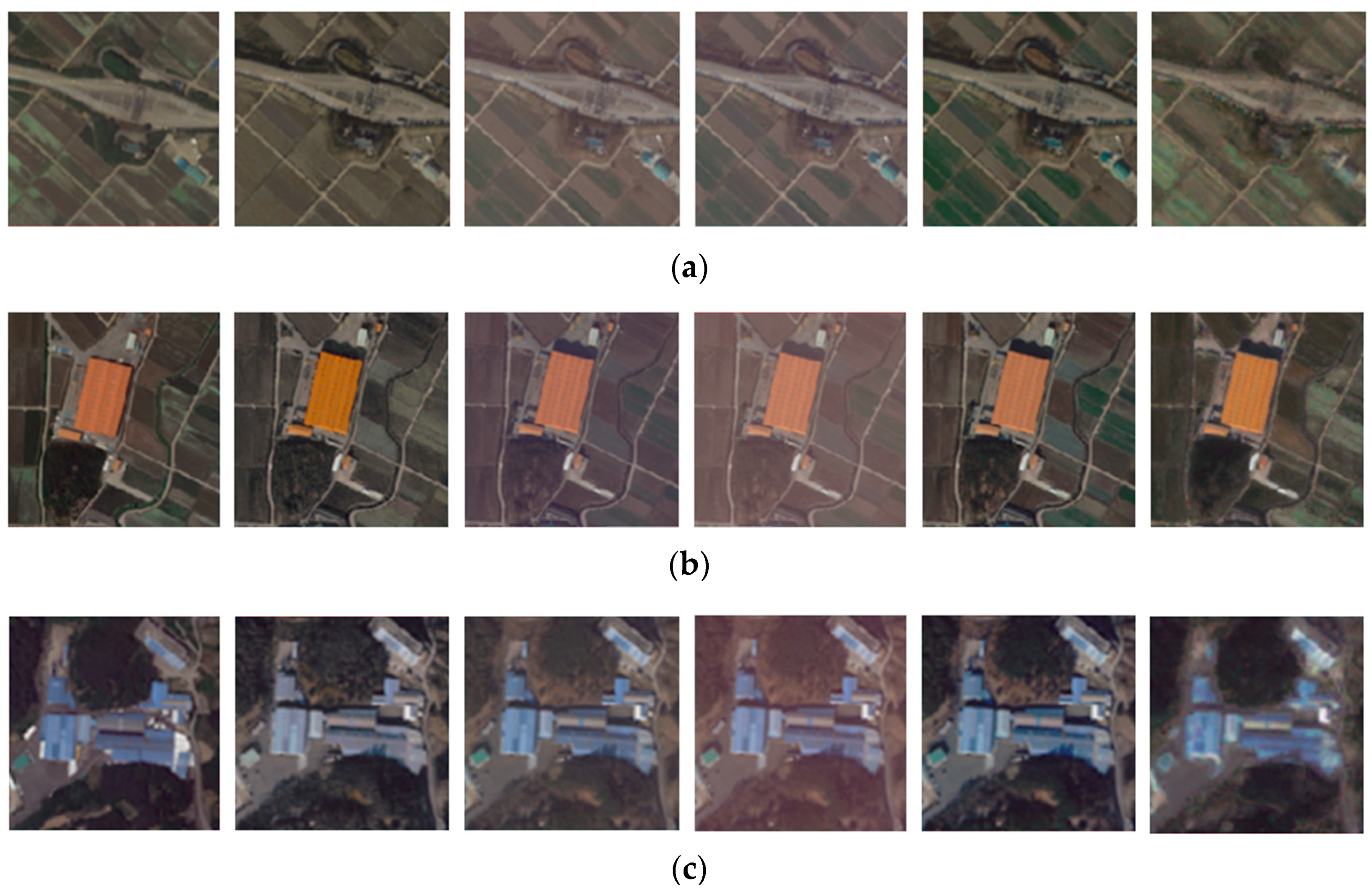
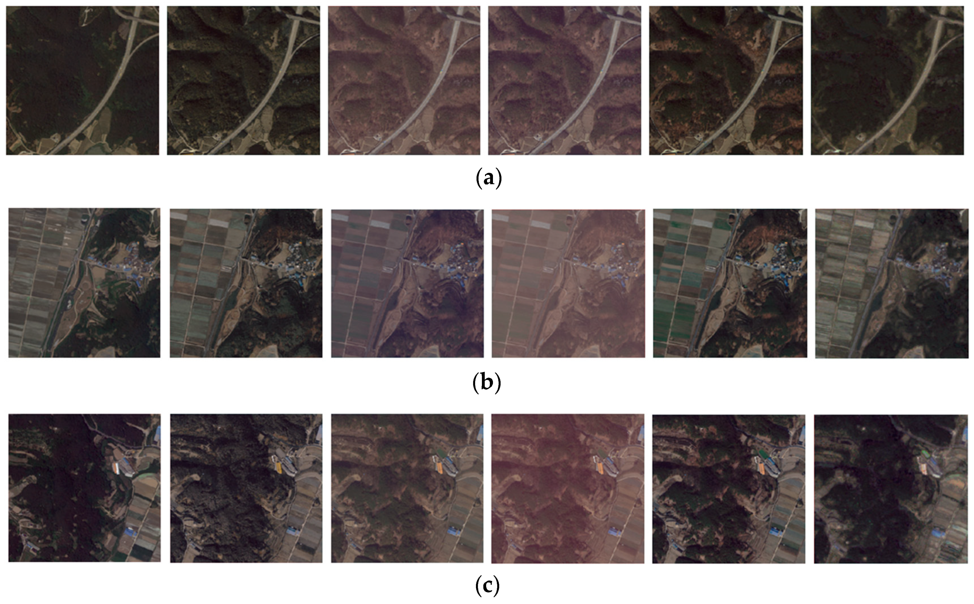
For the datasets used in this experiment, images that were obtained from the Korea Multi-Purpose Satellite (KOMPSAT)-3A, which is a high-resolution satellite sensor, are used. The product level is L1G, which is corrected for radiometric, sensor, and geometric distortions and projected to Universal Transverse Mercator (UTM). The KOMPSAT-3A multispectral images, consisting of four spectral bands with 2.2-m spatial resolution, were acquired on 30 October 2015 and 18 June 2016, which have significant differences in phenological characteristics. The images were co-registered from twenty-five ground control points that were identified in each image, and the warping method used was a first-order polynomial combined with nearest-neighbor resampling. The root mean squared error (RMSE) is less than 0.5 pixels. Furthermore, experiments are performed with subsets of 1200 × 1200 pixels, and a total of three sites are selected to achieve reasonable computation time. The details of the datasets used in this study are provided in Table 1, and the experimental images are shown in Figure 1, Figure 2 and Figure 3.
2.2. Methods
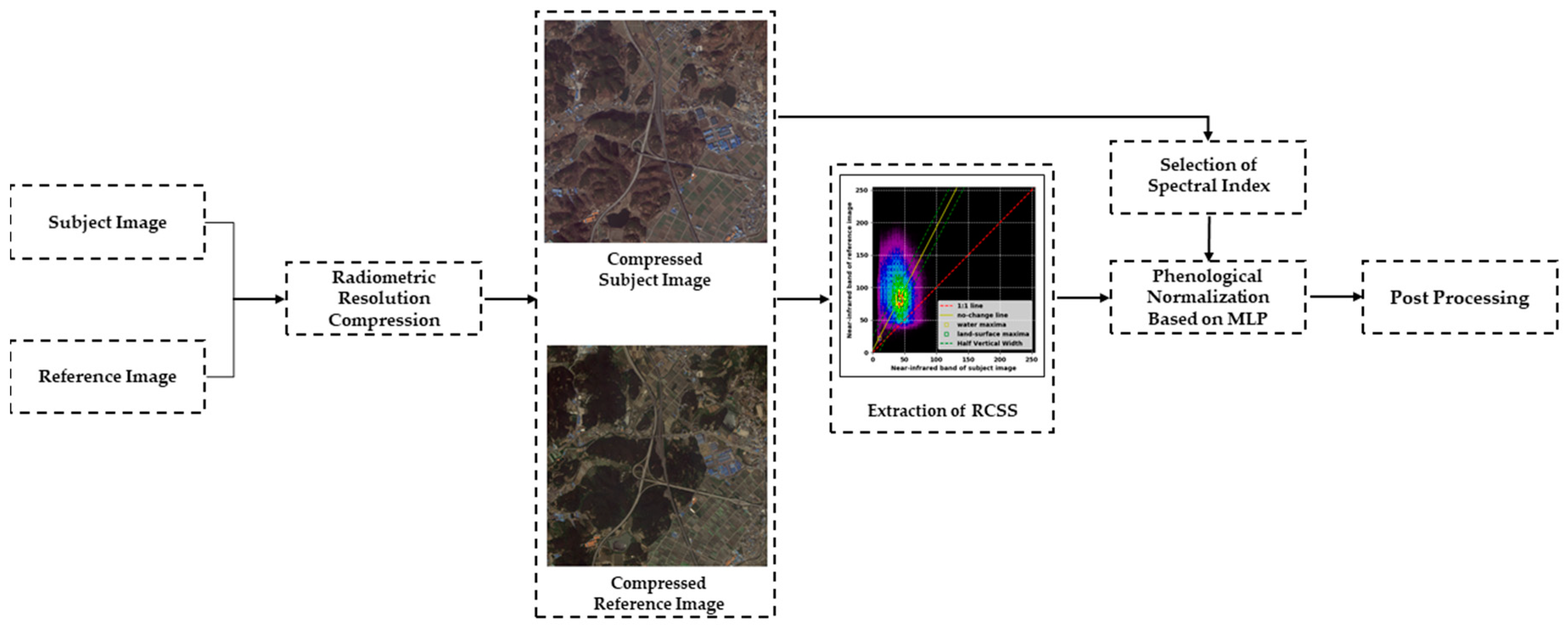
The proposed relative radiometric normalization framework can be decomposed into five steps: (1) radiometric resolution compression, (2) extraction of RCSS, (3) selection of a spectral index, (4) phenological normalization based on MLP, and (5) postprocessing, all of which are shown in Figure 4. The details of each step are described below.
2.2.1. Radiometric Resolution Compression
Radiometric resolution refers to the number of bit depth divisions, which represent the reflected energy of targets and influence the analysis of targets’ spectral features [35,36]. At this time, the greater the spatial resolution, the more the radiometric resolution can lead to additional noise in the image processing results [36]. Furthermore, a lower radiometric resolution reduces the computational complexity and it is more time efficient, while the difference in the information content in the high and low radiometric data is negligible [35]. Therefore, in this study, the radiometric resolution of the images is compressed while using the linear rescale method, and the range is taken from 8-bit to 14-bit [35,37]. The optimal radiometric resolution is set according to the results of multiple trials, with the goal to still balance the time cost and accuracy.
2.2.2. Extraction of RCSS
In this step, the RCSS extraction process is performed and, in order to ensure independence from operator performance effects, this process is automatically carried out. The proposed method is based on the NC method, which utilizes the scattergram between the near-infrared (NIR) bands of subject and reference images. This method locates the centers of the water and land-surface data clusters based on local maxima in the scattergram, where the water cluster center is not far from the origin, and the land-surface cluster center is near the center of the scattergram [19]. The coefficients for an NC line are computed once the above centers are determined, as shown in Equations (1) and (2):
where a is the gain, b is the offset, and are the respective water and land-surface data cluster centers of the subject image, and and are the respective water and land-surface data cluster centers of the reference image. Afterwards, a half vertical width (HVW) is defined via Equation (3):
where HPW is a half perpendicular width, which is commonly set to 10. Finally, the pixels inside the HVW are selected as the NC set, and they can be expressed via Equation (4):
where represents the pixels of the NIR band in the subject image and represents the pixels of the NIR band in the reference image.
2.2.3. Selection of the Spectral Index
A single pixel does not contain enough information and, therefore, features other than the pixel value must be considered to perform the phenological normalization [28,38,39]. The spectral indices are considered as features in this study, which is influenced by phenological properties [39,40,41]. At this time, the spectral indices calculated through reflectance, such as the normalized difference vegetation index, soil-adjusted vegetation index, or enhanced vegetation index, cannot be utilized, since the relative radiometric normalization is usually performed using the DN [3,41,42]. Therefore, the proposed method utilizes spectral indices that can be calculated through the DN values, among which the greenness indices of the excess green index (ExG), excess green minus excess red index (ExGR), vegetative index (VEG), color index of vegetation extraction (CIVE), and combined index (COM) are selected [43,44,45]. The greenness indices are obtained by converting the red-green-blue (RGB) color space to RGB chromatic coordinates, as defined in Equation (5):
where , , and are the blue, green, and red bands, respectively, and , , and are the chromatic coordinates of the blue, green, and red bands, respectively. Subsequently, the ExG, ExGR, VEG, CIVE, and COM are defined as in Equations (6)–(10):
At this time, feature selection is independently performed for each band, since the features affecting each band are different [25]. Furthermore, as the number of input features increases, the complexity of the model and noise increases, and thus it is important to select optimal features [46,47]. Therefore, one optimal spectral index for each band is selected in this study.
2.2.4. Phenological Normalization Based on Multilayer Perceptron
As mentioned above, the changes that are caused by the growth of vegetation are the most typical nonlinear changes in the radiometric characteristics. In other words, a nonlinear relationship is required in order to perform normalization for the radiometric differences as well as the phenological differences [25,26]. In this study, the nonlinear normalization is performed while using an MLP that is a representative algorithm for modeling nonlinear relationships [33,48]. The architecture of MLP consists of three units: the input layer, output layer, and hidden layer. The input layer is the first layer that transfers the initial data into the network, the output layer is the last layer that collects and transmits the results, and the hidden layer is an intermediate layer between the input and output layers that processes the data [31]. Each layer is composed of several neurons, where every neuron is connected to all of the neurons in the next layer through weighting [33]. When the input data are , a neuron k can be expressed, as in Equation (11):
where are the weights of neuron k, is the bias, is the activation function, and is the output of the neuron k. In this study, the input layer has two neurons, which represent the DN (or reflectance) and the optimal spectral index obtained above, and the output layer has one, which represents the normalized DN (or reflectance). Furthermore, the learning process is performed using a back-propagation algorithm that adjusts weights to minimize the error between the actual value and predicted value based on loss function. The process is continued until a predefined accuracy level or the maximum iterations are reached.
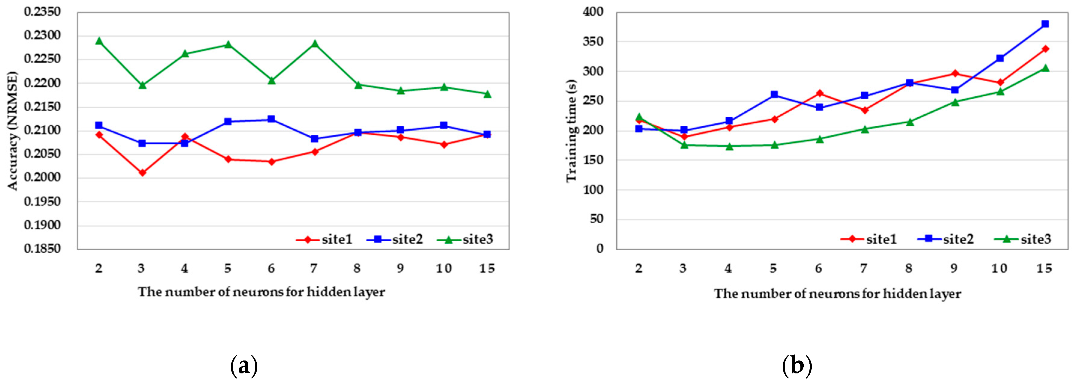
At this point, hyperparameters, such as the number of hidden layers, the number of neurons for hidden layers, learning rates, epochs, activation function, loss function, or optimizer, must be set up in order to construct the applicable MLP model [30]. The hyperparameters in the proposed method are selected based on experiences and experiments. As for the number of hidden layers, an increasing number causes a loss in the generalization power of the network, which might cause overfitting [49]. Furthermore, it increases the overall complexity of the algorithm and the training time [50]. Therefore, after considering the nature of the normalization, with limits of training time, only one hidden layer is considered [21,25]. As for the selection of the number of neurons for the hidden layer, the comparison experiments are conducted by setting the number of neurons to 2, 3, 4, 5, 6, 7, 8, 9, 10, and 15. The performance evaluation is conducted with normalization accuracy, normalized RMSE (NRMSE), which provides a lower value and better performance while taking the visual and quantitative aspects of the normalized image into account; Figure 5 shows the confirmatory results. The results show that, after three neurons, the time cost sharply increases, while the accuracy is not improved with the increase in neurons. Therefore, to balance the accuracy and time cost, three neurons for the hidden layer are selected in this experiment. As for the epochs and the learning rate, the figures 200 and are chosen, respectively, to prevent overfitting [34,51]. Furthermore, the activation function, loss function, and optimizer are selected as the rectified linear unit (ReLU), squared error, and adaptive moment estimation (ADAM), respectively. Table 2 summarizes all of the hyperparameters of the MLP and the values used in the proposed method.
2.2.5. Postprocessing
This step further adjusts the global statistical information for the phenological normalized image to normalize the radiometric properties. It is performed based on histogram matching, which matches the histogram’s distribution of the two images, so that the apparent distributions of the pixels correspond as closely as possible [21,39]. Histogram matching calculates the cumulative distribution functions of the subject and reference image histograms, and the reference pixels are then assigned to the subject pixels during their conversion back to a frequency distribution [52].
3. Results and Discussion
3.1. Comparisons of Normalization Results
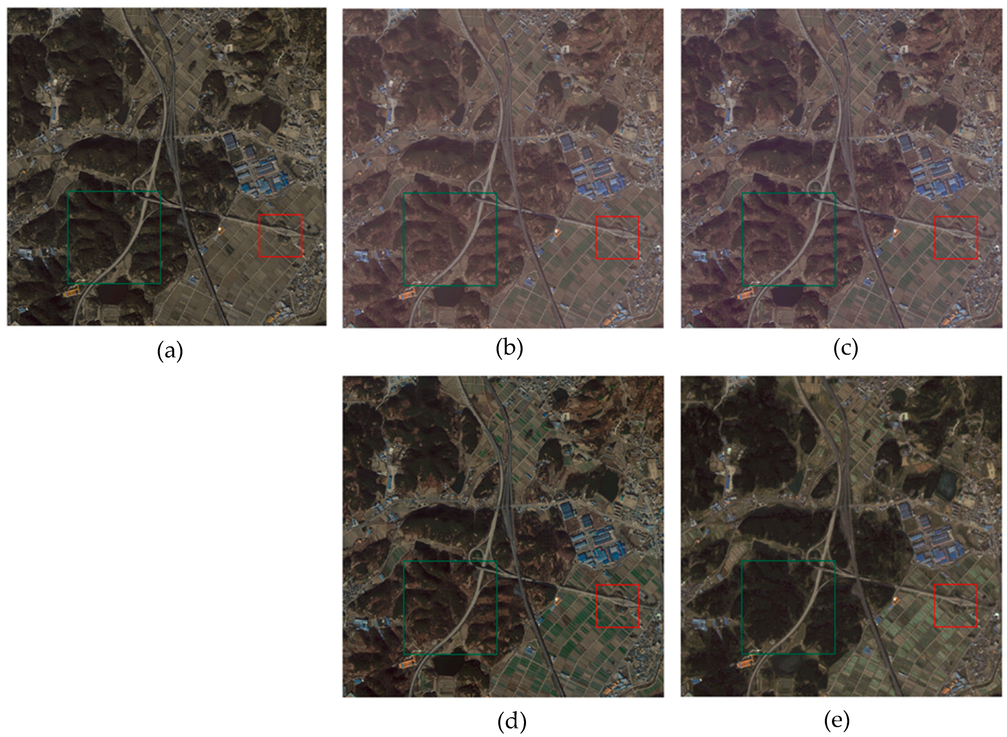
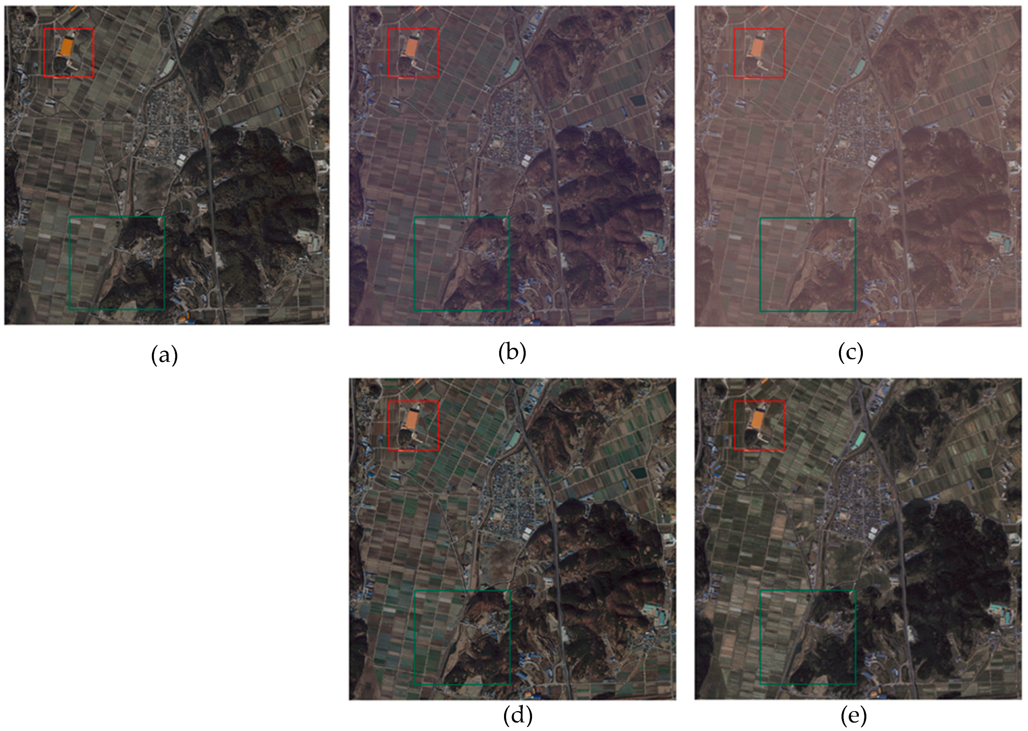
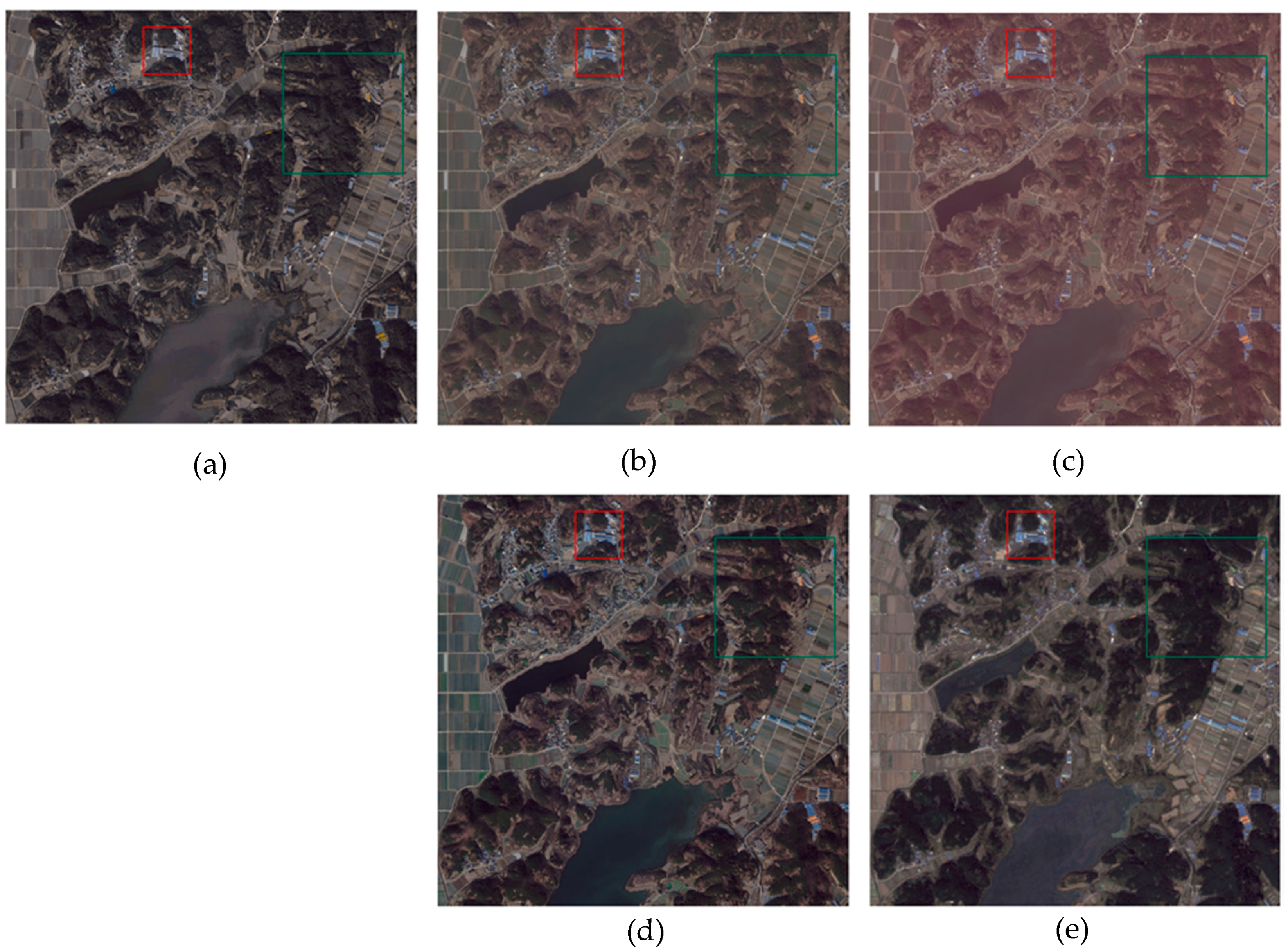
This section presents the normalization results of the proposed algorithm and then compares them with the results of a conventional algorithm. First, our proposed normalization process is performed step-by-step for the experimental images, in which the radiometric resolution is compressed to 8-bits, and the spectral indices of the blue, green, red, and NIR bands are selected as ExG, COM, ExGR, and ExG, respectively. Subsequently, the results of our proposed method are compared with the conventional methods (MS, NC, histogram matching, and random forest (RF)) to evaluate them visually and quantitatively, and Figure 6, Figure 7 and Figure 8 show the results for each experimental image.
From the overall visual inspection, the normalization of the proposed method is shown to be better than that of the conventional methods. MS and NC, which are regression-based methods, assume that the relationship between the subject and reference images is linear. However, as shown in the results, neither the phenological properties nor the radiometric properties are normalized. In other words, it can be confirmed that it is not appropriate to assume a linear relationship in the case of high-resolution images, in which vegetation changes exist. In the case of histogram matching, it is a representative nonlinear normalization method, which is based on global statistical information. Overall, the radiometric properties are normalized, while the normalization for the phenological properties is not performed at all. That is, when only statistical information is used, it is possible to normalize the radiometric properties, but there is a limit to phenological normalization. RF is a nonlinear method that is performed through RF regression, which uses neighbor information-based features, such as the mean, variance, and gray-level co-occurrence matrix as the training input values [25]. The results of this method show that the radiometric and phenological normalizations are performed, but spectral distortion is present. Furthermore, blurriness occurs in the results due to the neighbor information-based features, which results in some loss of detail, especially on linear objects. On the other hand, our proposed method shows that the radiometric and phenological normalizations are properly performed, and there is no spectral distortion or blurriness in the results.
To verify the radiometric and phenological normalization results in detail, some regions are selected and enlarged, with red rectangles representing the built-up areas and green rectangles representing the vegetation areas. Figure 9 shows built-up areas, which represent the radiometric properties, consist of roads and the roofs of buildings, and the enlarged areas for each normalization result. For roads, the proposed method normalizes the radiometric properties in such a way that the image is the closest in consistency with the reference image, while, in the case of roofs, the results vary for the site. For site 2, showing a relatively large roof, the radiometric properties normalized through the proposed method show the most similarity with those of the reference image, whereas for site 3, showing several small roofs, the proposed method displays some turbidity when compared to other methods. In other words, roofs are affected by their objective size, which is judged according to its geometric distortion. Large-sized objects can be trained properly, even in the presence of geometric distortion, while small-sized objects acquire the characteristic of other surrounding objects, which adversely affects training. For vegetation areas, phenological properties, such as forests, grass, and crops, are included, and Figure 10 shows the corresponding enlarged areas. In the case of forests, it is confirmed that the areas without vegetation due to the phenological properties in the subject image are normalized to the same phenological properties as the reference image at all sites. For grass and crops, the performance of normalization is somewhat less than that for forests due to the heterogenous characteristics, but it contains the characteristics of the reference image as a whole.
Although visual inspection is a straightforward and direct manner of comparison, it is highly subjective; thus, quantitative evaluations of each method are further performed based on NRMSE. The NRMSE is defined as in Equations (12) and (13):
where is RCSSs in the normalized image of band ; is the RCSSs in the reference image of band ; is the total number of RCSSs; and, is the mean of RCSSs in the reference image of band i. Table 3 shows the NRMSE for the results of the proposed method and the conventional methods.
As a result of the quantitative evaluation through NRMSE, although all of the methods show a generally reduced radiometric variation, the proposed method displays the highest performance improvement among them. When compared with the performance of the subject image, on average, the proposed method improves it by 32.85–33.96%, whereas MS, NC, histogram matching, and RF are improved by 18.26–21%, 21.95–24.48%, 20.87–22.87%, and 25.12–28.82%, respectively. This means that the normalized image of the proposed method has the highest accuracy and it is similar to the radiometric and phenological properties of the reference image. In other words, the visual and quantitative evaluations both confirm that it would be useful to carry out normalization with the proposed method when phonological differences exist for the high-resolution images.
3.2. Influence of the Radiometric Resolution
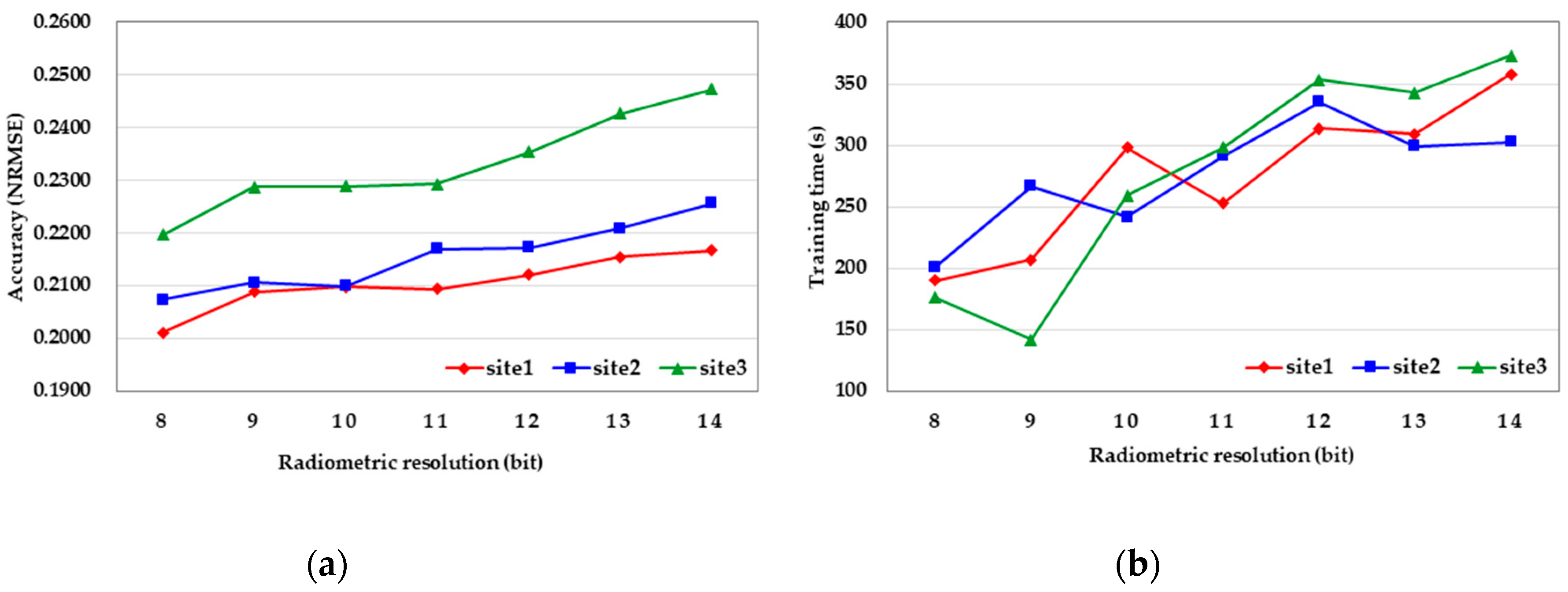
The radiometric resolution represents the range that is normalized when performing the proposed method, which is closely related to the complexity and time cost. Therefore, the performance evaluation according to the radiometric resolution is performed and the range is set from 8-bit to 14-bit, as mentioned earlier. The average of the NRMSE in the entire band is calculated and considered with the training time, as shown in Figure 11. In the case of site 1, the performance of 8-bit is the highest, and the training time is the lowest, while the performance of 14-bit is the lowest and the training time is the highest. At site 2, 8-bit has the highest performance and the lowest training time, and 14-bit has the lowest performance (same as site 1), while the training time is the highest in 12-bit mode. The best performance at site 3 is also 8-bit, but the lowest training time is 9-bit, and the lowest performance and the highest training time are the same as at site 1. Overall, similar results are obtained at all sites. As the radiometric resolution increases, the performance decreases, and the training time and complexity increase. In other words, high radiometric resolution leads to overtraining in the radiometric normalization, which requires more complex computations and it interferes with the performance improvements. Thus, 8-bit is selected as the optimal radiometric resolution in this study.
3.3. Influence of the Spectral Index
The spectral index serves as a complement to the DN or reflectance for the phenological normalization, which is a key parameter in this study. A performance evaluation of each spectral index for each band is performed in order to select the optimal spectral index for each band, as shown in Table 4. It can be found that the same tendency is shown at all sites. ExG show high performance in the blue and NIR bands, while the performance in the red band is relatively low. In the case of ExGR, the performance of the red band is satisfactory, while the blue, green, and NIR bands are somewhat inferior in performance. Furthermore, VEG has the lowest performance overall, and CIVE has a normal performance as a whole, but it does not show optimized performance. On the other hand, Com shows the highest performance in the green band, demonstrating reasonable performance as a whole. In other words, it is confirmed that there is a considerable difference in the influence of each spectral index on each band. Therefore, ExG, COM, ExGR, and ExG are selected as the optimal spectral indices for the blue, green, red, and NIR bands, respectively.
3.4. Additional Dataset
Additional KOMPSAT-3 and KOMPSAT-3A data with different phenological properties are added in order to verify the robustness of the proposed method. The experimental area is Seoul, which mainly contains built-up areas and forests. KOMPSAT-3 and KOMPSAT-3A have the same spectral response functions and practical spectral ranges as the bands that are affected by atmospheric constituents and the surface, where the main difference between them is only the spatial resolution [53]. Therefore, the experiment is performed by resampling KOMPSAT-3 at 2.2 m, which is the same resolution as KOMPSAT-3A, and the size of the images is set to 2000 × 1500 pixels. Figure 12 provides the bitemporal images and normalization results. From a visual inspection, it can be seen that the normalization of the radiometric and phenological properties are properly performed. In particular, the spectral characteristics of the forest area are normalized to be the same as those of the reference image. Furthermore, as shown in Table 5, the performance for the additional area is similar to that in the previous results. In other words, it can be confirmed that the proposed method can also achieve satisfactory results with the additional dataset.
4. Conclusions
This paper proposes a novel method for performing the normalization of radiometric properties due to atmospheric conditions and phenological properties due to changes in vegetation for high-resolution satellite images. MLP forms the basis of the proposed method, and a nonlinear relationship is assumed in order to normalize the aforementioned properties, in contrast to the approach that is used by conventional relative radiometric normalization algorithms. The proposed method performs radiometric resolution compression for subject and reference images, and 8-bit is selected when considering the complexity and time cost. Subsequently, RCSS is extracted based on the NC method, and a spectral index for each band is selected (ExG, COM, ExGR, and ExG). Phenological normalization is performed by establishing a nonlinear relationship through MLP. Regarding MLP, the number of hidden layers is fixed at one, when considering the algorithm generalization and the training time limits, while the number of the layer’s neurons is determined through experiments. Generally, the higher the number of neurons for the hidden layer, the greater the network capacity required to train the model. However, in this study, it is confirmed that, as the number of neurons for hidden layer increased, the training time increased, while the accuracy decreased. In other words, networks with high complexity have poor generalizations and adverse effects as compared to small and simple networks. Thus, three neurons for the hidden layer are selected. Finally, the global radiometric properties are adjusted through postprocessing.
The proposed method is then compared with conventional methods (MS, NC, histogram matching, and RF), which shows superior results via both visual inspection and quantitative evaluation. Visually, this finding suggests that the concepts that are mentioned above are suited to normalize radiometric and phenological properties. The methods that assume linear relationships cannot normalize the radiometric and phenological properties at all. When assuming a nonlinear relationship, if only statistical information is used, the radiometric properties are normalized, but phenological normalization cannot be performed. In the RF approach, radiometric and phenological normalizations are performed, but with a loss of information, such as spectral distortion and blurriness, which is due to neighbor information-based features. Furthermore, to analyze the radiometric and phenological properties in detail, some areas are enlarged. In terms of the radiometric properties, homogeneous features, such as roads, show better performance when compared to heterogenous features, such as roofs, which are constructed with a variety of materials. The heterogenous features are especially affected by object size in the presence of geometric distortion. Similar tendencies are observed in the case of phenological properties, where the normalization of the homogeneous features, such as forests, is better than of the heterogenous features, such as grass and crops. Quantitatively, the NRMSE of the proposed method is the most improved when compared with the performance of the subject image. In other words, the normalized image of the proposed method is the most similar to the radiometric and phenological properties of the reference image, which represents the applicability of the proposed method as a preprocessing step in change detection when vegetation changes exist in multi-temporal images.
Future works will focus on the following aspects. First, acquiring enough images for each season, period, and sensor to more thoroughly evaluate the various characteristics should be undertaken to perform additional verification. Second, spectral indices excluding those used in this study should be considered, and further analysis on the effect of their combinations should be studied. Third, further research on the hyperparameters, such as the number of hidden layers and the number of neurons, should be conducted to achieve the most optimal normalization results. Finally, the applicability of change detection should be investigated by applying normalized images from the proposed method to change detection.
Author Contributions
Conceptualization, Y.D.E.; methodology, D.K.S.; software, D.K.S.; validation, D.K.S.; formal analysis, D.K.S.; investigation, D.K.S.; resources, D.K.S.; data curation, Y.D.E.; writing—original draft preparation, Y.D.E.; writing—review and editing, Y.D.E.; visualization, D.K.S.; supervision, Y.D.E.; project administration, Y.D.E.; funding acquisition, Y.D.E.
Funding
This research was supported by a grant (19SIUE-B148326-02) from Satellite Information Utilization Center Establishment Program by Ministry of Land, Infrastructure and Transport of Korean government.
Conflicts of Interest
The authors declare no conflict of interest.
References
- Zhong, C.; Xu, Q.; Li, B. Relative Radiometric Normalization for Multitemporal Remote Sensing Images by Hierarchical Regression. IEEE Geosci. Remote Sens. Lett. 2016, 13, 217–221. [Google Scholar] [CrossRef]
- Hong, G.; Zhang, Y.A. A Comparative Study on Radiometric Normalization Using High Resolution Satellite Images. Int. J. Remote Sens. 2008, 29, 425–438. [Google Scholar] [CrossRef]
- Zhou, H.; Liu, S.; He, J.; Wen, Q.; Song, L.; Ma, Y. A New Model for the Automatic Relative Radiometric Normalization of Multiple Images with Pseudo-Invariant Features. Int. J. Remote Sens. 2016, 37, 4554–4573. [Google Scholar] [CrossRef]
- Chen, X.; Vierling, L.; Deering, D. A Simple and Effective Radiometric Correction Method to Improve Landscape Change Detection Across Sensors and Across Time. Remote Sens. Environ. 2005, 98, 63–79. [Google Scholar] [CrossRef]
- Kim, D.S.; Pyeon, M.W.; Eo, Y.D.; Byun, Y.G.; Kim, Y.I. Automatic Pseudo-Invariant Feature Extraction for the Relative Radiometric Normalization of Hyperion Hyperspectral Images. GIsci. Remote Sens. 2012, 49, 755–773. [Google Scholar] [CrossRef]
- Song, C.; Woodcock, C.E.; Seto, K.C.; Lenny, M.P.; Macomber, S.A. Classification and Change Detection Using Landsat TM Data: When and How to Correct Atmospheric Effects? Remote Sens. Environ. 2001, 75, 230–244. [Google Scholar] [CrossRef]
- Du, Y.; Teillet, P.M.; Cihlar, J. Radiometric Normalization of Multitemporal High-Resolution Satellite Images with Quality Control for Land Cover Change Detection. Remote Sens. Environ. 2002, 82, 123–134. [Google Scholar] [CrossRef]
- Bao, N.; Lechner, A.M.; Fletcher, A.; Mellor, A.; Mulligan, D.; Bai, Z. Comparison of Relative Radiometric Normalization Methods Using Pseudo Invariant Features for Change Detection Studies in Rural and Urban Landscapes. J. Appl. Remote Sens. 2012, 6, 1–18. [Google Scholar] [CrossRef]
- Schroeder, T.A.; Cohen, W.B.; Song, C.; Canty, M.J.; Yang, J. Radiometric Correction of Multi-Temporal Landsat Data for Characterization of Early Successional Forest Patterns in Western Oregon. Remote Sens. Environ. 2006, 103, 16–26. [Google Scholar] [CrossRef]
- Hall, F.G.; Strebel, D.E.; Nickson, J.E.; Geoets, S.J. Radiometric Rectification: Toward a Common Radiometric Response Among Multidate, Multisensor Images. Remote Sens. Environ. 1991, 35, 11–27. [Google Scholar] [CrossRef]
- Liu, Y.; Yano, T.; Nishiyama, S.; Kimura, R. Radiometric Correction for Linear Change-Detection Technique: Analysis in Bi-Temporal Space. Int. J. Remote Sens. 2007, 28, 5143–5157. [Google Scholar] [CrossRef]
- Biday, S.G.; Bhosle, U. Radiometric Correction of Multitemporal Satellite Imagery. J. Comput. Sci. 2010, 6, 201–213. [Google Scholar] [CrossRef]
- Canty, M.J.; Nielsen, A.A.; Schmidt, M. Automatic Radiometric Normalization of Multitemporal Satellite Imagery. Remote Sens. Environ. 2004, 91, 441–451. [Google Scholar] [CrossRef]
- Vicente-Serrano, S.M.; Perez-Cabello, F. Assessment of Radiometric Correction Techniques in Analyzing Vegetation Variability and Change Using Time Series of Landsat Images. Remote Sens. Environ. 2008, 112, 3916–3934. [Google Scholar] [CrossRef]
- Yang, X.J.; Lo, C.P. Relative Radiometric Normalization Performance for Change Detection from Multi-Date Satellite Images. Photogramm. Eng. Remote Sens. 2000, 66, 967–980. [Google Scholar]
- Yuan, D.; Elvidge, C.D. Comparison of Relative Radiometric Normalization Techniques. ISPRS J. Photogramm. Remote Sens. 1996, 51, 117–126. [Google Scholar] [CrossRef]
- Chavez, P.S., Jr. An Improved Dark-Object Subtraction Technique for Atmospheric Scattering Correction of Multispectral Data. Remote Sens. Environ. 1988, 24, 459–479. [Google Scholar] [CrossRef]
- Schott, J.R.; Salvaggio, C.; Volhock, W.J. Radiometric Scene Normalization Using Pseudo-Invariant Features. Remote Sens. Environ. 1988, 26, 1–14. [Google Scholar] [CrossRef]
- Elvidge, C.D.; Yuan, D.; Weerackoon, R.D.; Lunetta, R.S. Relative Radiometric Normalization of Landsat Multispectral Scanner (MSS) Data Using an Automatic Scattergram Controlled Regression. Photogramm. Eng. Remote Sens. 1995, 61, 1255–1260. [Google Scholar]
- Ya’allah, S.M.; Saradjian, M.R. Automatic Normalization of Satellite Images Using Unchanged Pixels within Urban Areas. Inf. Fusion. 2005, 6, 235–241. [Google Scholar] [CrossRef]
- Sadeghi, V.; Ebadi, H.; Ahmadi, F.F. A New Model for Automatic Normalization of Multitemporal Satellite Images Using Artificial Neural Network and Mathematical Methods. Appl. Math. Modell. 2013, 37, 6437–6445. [Google Scholar] [CrossRef]
- Rahman, M.M.; Hay, G.J.; Couloigner, I.; Hemachandran, B.; Bailin, J. An Assessment of Polynomial Regression Techniques for the Relative Radiometric Normalization (RRN) of High-Resolution Multi-Temporal Airborne Thermal Infrared (TID) Imagery. Remote Sens. 2014, 6, 11810–11828. [Google Scholar] [CrossRef]
- Hang, R.; Liu, Q.; Song, H.; Sun, Y.; Zhu, F.; Pei, H. Graph Regularized Nonlinear Ridge Regression for Remote Data Analysis. IEEE J. Sel. Top. Appl. Earth Obs. Remote Sens. 2017, 10, 277–285. [Google Scholar] [CrossRef]
- Kim, H.J.; Seo, D.K.; Eo, Y.D.; Jeon, M.C.; Park, W.Y. Multi-Temporal Nonlinear Regression Method for Landsat Image Simulation. KSCE J. Civ. Eng. 2019, 23, 777–787. [Google Scholar] [CrossRef]
- Seo, D.K.; Kim, Y.H.; Eo, Y.D.; Park, W.Y.; Park, H.C. Generation of Radiometric, Phenological Normalized Images Based on Random Forest Regression for Change Detection. Remote Sens. 2017, 9, 1163. [Google Scholar] [CrossRef]
- Bai, Y.; Tang, P.; Hu, C. kCCA Transformation -Based Radiometric Normalization of Multi-Temporal Satellite Images. Remote Sens. 2018, 10, 432. [Google Scholar] [CrossRef]
- Zheng, Y.; Zhang, J.; van Genderen, J.L. Change Detection Approach to SAR and Optical Image Integration. Int. Arch. Photogramm. Remote Sens. 2008, XXXVII Pt B7, 1077–1084. [Google Scholar]
- Seo, D.K.; Kim, Y.H.; Eo, Y.D.; Lee, M.H.; Park, W.Y. Fusion of SAR and Multispectral Images Using Random Forest Regression for Change Detection. ISPRS Int. J. Geo-Inf. 2018, 7, 401. [Google Scholar] [CrossRef]
- Ji, C.Y. Land-Use Classification of Remotely Sensed Data Using Kohonen Self-Organizing Feature Map Neural Network. Photogramm. Eng. Remote Sens. 2000, 66, 1451–1460. [Google Scholar]
- Hu, X.; Weng, Q. Estimating Impervious Surfaces from Medium Spatial Resolution Imagery Using the Self-Organizing Map and Multi-Layer Perceptron Neural Networks. Remote Sens. Environ. 2009, 113, 2089–2102. [Google Scholar] [CrossRef]
- Taravat, A.; Proud, S.; Peronaci, S.; Frate, F.D.; Oppelt, N. Multilayer Perceptron Neural Networks Model for Meteosat Second Generation SEVIRI Daytime Cloud Masking. Remote Sens. 2015, 7, 1529–1539. [Google Scholar] [CrossRef] [Green Version]
- Thakur, A.; Mishra, D. Hyperspectral Image Classification Using Multilayer Perception Neural Network & Functional Link ANN. In Proceedings of the 2017 7th international Conference on Cloud Computing, Data Science & Engineering-Confluence, Noida, India, 12–13 January 2017; pp. 639–642. [Google Scholar]
- Patra, S.; Ghosh, S.; Ghosh, A. Change Detection of Remote Sensing Images with Semi-Supervised Multilayer Perceptron. Fundam. Inf. 2008, 84, 429–442. [Google Scholar]
- Jiang, W.; He, G.; Long, T.; Ni, Y.; Liu, H.; Peng, Y.; Lv, K.; Wang, G. Multilayer Perceptron Neural Network for Surface Water Extraction in Landsat 8 OLI Satellite Images. Remote Sens. 2018, 10, 755. [Google Scholar] [CrossRef]
- Verde, N.; Mallinis, G.; Tsakiri-Strati, M.; Georgiadis, C.; Patias, P. Assessment of Radiometric Resolution Impact on Remote Sensing Data Classification Accuracy. Remote Sens. 2018, 10, 1267. [Google Scholar] [CrossRef]
- Miyoshi, G.T.; Imai, N.N.; Tommaselli, A.M.G.; Honkavaara, E. Impact of Reduction of Radiometric Resolution in Hyperspectral Images Acquired over Forest Field. Int. Arch. Photogramm. Remote Sens. Spat. Inf. Sci. 2018, XLII-1, 301–305. [Google Scholar] [CrossRef]
- Alonso, C.; Tarquis, A.M.; Zuniga, I.; Benito, R.M. Spatial and Radiometric Characterization of Multi-Spectrum Satellite Images through Multi-Fractal Analysis. Nonlinear Process. Geophys. 2017, 24, 141–155. [Google Scholar] [CrossRef]
- Seo, D.K.; Kim, Y.H.; Eo, Y.D.; Park, W.Y. Learning-Based Colorization of Grayscale Aerial Images Using Random Forest Regression. Appl. Sci. 2018, 7, 1269. [Google Scholar] [CrossRef]
- Seo, D.K.; Eo, Y.D. Relative Radiometric Normalization for High-Resolution Satellite Imagery Based on Multilayer Perceptron. J. Korean Soc. Surv. Geod. Photogramm Cartogr. 2018, 36, 515–523. [Google Scholar] [CrossRef]
- Motohka, T.; Nasahara, K.N.; Oguma, H.; Tsuchida, S. Applicability of Green-Red Vegetation Index for Remote Sensing of Vegetation Phenology. Remote Sens. 2010, 2, 2369–2387. [Google Scholar] [CrossRef] [Green Version]
- Xue, J.; Su, B. Significant Remote Sensing Vegetation Indices: A Review of Developments and Applications. J. Sens. 2017, 2017, 1353691. [Google Scholar] [CrossRef]
- Carvalho, O.A.D.; Guimaraes, R.F.; Silva, N.C.; Gillespie, A.R.; Gomes, R.A.T.; Silva, C.E.; Carvalho, A.P.F.D. Radiometric Normalization of Temporal Images Combining Automatic Detection of Pseudo-Invariant Features from the Distance and Similarity Spectral Measures, Density Scatterplot Analysis and Robust Regression. Remote Sens. 2013, 5, 2763–2794. [Google Scholar] [CrossRef]
- Yang, W.; Wang, S.; Zhao, X.; Zhang, J.; Feng, J. Greenness Identification Based on HSV Decision Tree. Inf. Process. Agric. 2015, 2, 149–160. [Google Scholar] [CrossRef]
- Sonnentag, O.; Hufkens, K.; Teshera-Sterne, C.; Young, A.M.; Friedl, M.; Braswell, B.H.; Millinam, T.; O’Keefe, J.; Richardson, A.D. Digital Repeat Photography for Phenological Research in Forest Ecosystems. Agric. For. Meteorol. 2012, 152, 159–177. [Google Scholar] [CrossRef]
- Larrinaga, A.R.; Brotons, L. Greenness Indices from a Low-Cost UAV Imagery as Tools for Monitoring Post-Fire Recovery. Drones 2019, 3, 6. [Google Scholar] [CrossRef]
- Kwak, N.J.; Choi, C.H. Input Feature Selection for Classification Problems. IEEE Trans. Neural Netw. 2002, 13, 143–159. [Google Scholar] [CrossRef]
- Koo, J.H.; Seo, D.K.; Eo, Y.D. Variable Importance Assessment for Colorization of Grayscale Aerial Images Based on Random Forest, Adaptive Boosting and Stochastic Gradient Boosting. Disaster Adv. 2018, 11, 22–29. [Google Scholar]
- Reifman, M.M.; Feldman, E.E. Multilayer Perceptron for Nonlinear Programming. Comput. Oper. Res. 2002, 29, 1237–1250. [Google Scholar] [CrossRef]
- Rodriguez-Galiano, V.; Sanchez-Castillo, M.; Chica-Olmo, M.; Chica-Rivas, M. Machine Learning Predictive Models for Mineral Prospectivity: An Evaluation of Neural Networks, Random Forest, Regression Trees and Support Vector Machines. Ore Geol. Rev. 2015, 71, 804–818. [Google Scholar] [CrossRef]
- Karsoliya, S. Approximating Number of Hidden Layer Neurons in Multiple Hidden Layer BPNN Architecture. Int. J. Eng. Trends Technol. 2012, 3, 714–717. [Google Scholar]
- Sumsion, G.R.; Bradshaw, M.S.; Hill, K.T.; Pinto, L.D.G.; Piccolo, S.R. Remote Sensing Tree Classification with a Multilayer Perceptron. PeerJ 2019, 7, 1–13. [Google Scholar] [CrossRef]
- Hermel, E.H.; Ruefenacht, B. A Comparison of Radiometric Normalization Methods When Filling Cloud Gaps in Landsat Imagery. Can. J. Remote Sen. 2007, 33, 325–340. [Google Scholar] [CrossRef]
- Yeom, J.M.; Ko, J.H.; Hwang, J.S.; Lee, C.S.; Chou, C.U.; Jeong, S.T. Updating Absolute Radiometric Characteristics for KOMPSAT-3 and KOMPSAT-3A Multispectral Imaging Sensors Using Well-Characterized Pseudo-Invariant Tarps and Microtops II. Remote Sens. 2018, 10, 697. [Google Scholar] [CrossRef]
Figure 1.
The experimental images from site 1: (a) subject image acquired on 30 October 2015, (b) reference image acquired on 18 June 2016.
Figure 1.
The experimental images from site 1: (a) subject image acquired on 30 October 2015, (b) reference image acquired on 18 June 2016.

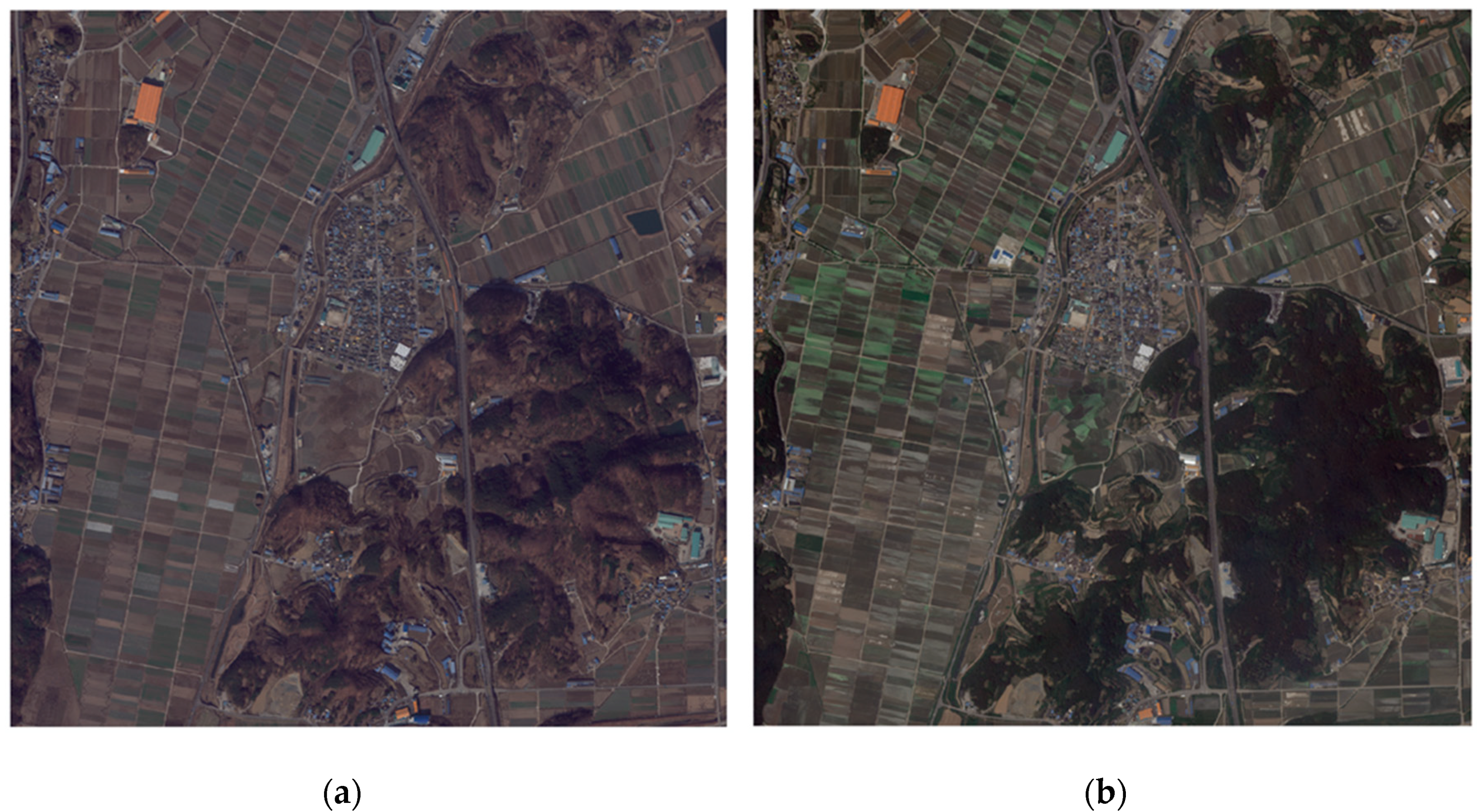
Figure 2.
The experimental images from site 2: (a) subject image acquired on 30 October 2015, (b) reference image acquired on 18 June 2016.
Figure 2.
The experimental images from site 2: (a) subject image acquired on 30 October 2015, (b) reference image acquired on 18 June 2016.

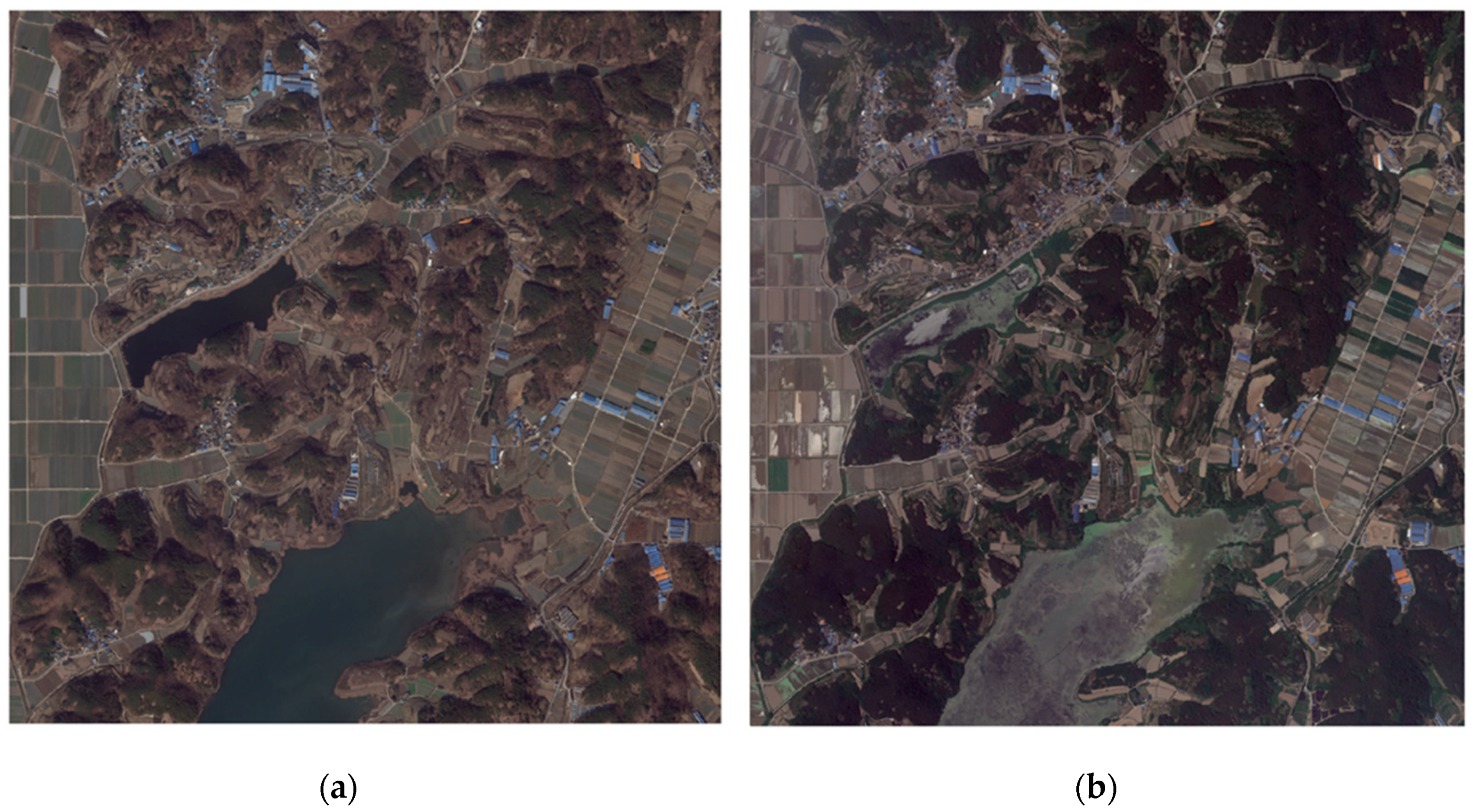
Figure 3.
The experimental images from site 3: (a) subject image acquired on 30 October 2015, (b) reference image acquired on 18 June 2016.
Figure 3.
The experimental images from site 3: (a) subject image acquired on 30 October 2015, (b) reference image acquired on 18 June 2016.

Figure 4.
Flowchart of the proposed method.

Figure 5.
Experiments regarding the number of neurons for the hidden layer: (a) accuracy by setting different neurons, (b) training time by setting different neurons.
Figure 5.
Experiments regarding the number of neurons for the hidden layer: (a) accuracy by setting different neurons, (b) training time by setting different neurons.

Figure 6.
Comparison with the results of relative radiometric normalization for site 1: (a) proposed method (b) MS, (c) NC, (d) histogram matching, (e) RF.
Figure 6.
Comparison with the results of relative radiometric normalization for site 1: (a) proposed method (b) MS, (c) NC, (d) histogram matching, (e) RF.

Figure 7.
Comparison with the results of relative radiometric normalization for site 2: (a) proposed method (b) MS, (c) NC, (d) histogram matching, (e) RF.
Figure 7.
Comparison with the results of relative radiometric normalization for site 2: (a) proposed method (b) MS, (c) NC, (d) histogram matching, (e) RF.

Figure 8.
Comparison with the results of relative radiometric normalization for site 3: (a) proposed method (b) MS, (c) NC, (d) histogram matching, (e) RF.
Figure 8.
Comparison with the results of relative radiometric normalization for site 3: (a) proposed method (b) MS, (c) NC, (d) histogram matching, (e) RF.

Figure 9.
Enlargement of the built-up area marked with a red rectangle: (a) site 1, (b) site 2, (c) site 3. From left to right: reference image, proposed method, MS, NC, histogram matching, and RF.
Figure 9.
Enlargement of the built-up area marked with a red rectangle: (a) site 1, (b) site 2, (c) site 3. From left to right: reference image, proposed method, MS, NC, histogram matching, and RF.

Figure 10.
Enlargement of the vegetation area marked with a green rectangle: (a) site 1, (b) site 2, (c) site 3. From left to right: reference image, proposed method, MS, NC, histogram matching, and RF.
Figure 10.
Enlargement of the vegetation area marked with a green rectangle: (a) site 1, (b) site 2, (c) site 3. From left to right: reference image, proposed method, MS, NC, histogram matching, and RF.

Figure 11.
Experiments on the radiometric resolution: (a) accuracy by setting different radiometric resolutions, (b) training time by setting different radiometric resolutions.
Figure 11.
Experiments on the radiometric resolution: (a) accuracy by setting different radiometric resolutions, (b) training time by setting different radiometric resolutions.

Figure 12.
The experimental images for the additional dataset: (a) subject image acquired on 23 February 2017, (b) reference image acquired on 09 October 2015, and (c) normalization result of the proposed method.
Figure 12.
The experimental images for the additional dataset: (a) subject image acquired on 23 February 2017, (b) reference image acquired on 09 October 2015, and (c) normalization result of the proposed method.


Table 1.
Specifications of the satellite sensors.
| Sensor | KOMPSAT-3A (subject image) | KOMPSAT-3A (reference image) |
| Location | Changnyeong-gun (Korea) | |
| Date | 30 Oct. 2015 | 18 Jun. 2016 |
| Spatial resolution (m) | 2.2 (multispectral) | |
| Spectral resolution (nm) | Blue: 450–510 Green: 520–600 Red: 630–690 Near-infrared: 760–900 | |
| Radiometric resolution | 14-bit | |
| Image size (pixels) | 1200 × 1200 | |
Table 2.
The hyperparameters of the multilayer perceptron (MLP).
| Hyperparameter | Value |
|---|---|
| Number of input variables | 2 |
| Number of hidden layers | 1 |
| Number of neurons in the hidden layer | 3 |
| Number of neurons in the output layer | 1 |
| Activation function | ReLU |
| Loss function | Squared error |
| Optimizer | ADAM |
| Learning rate | 10−4 |
| Training epochs | 200 |
Table 3.
Normalized root mean squared error (NRMSE) of relative radiometric normalization results.
| Site | Method | Band 1 | Band 2 | Band 3 | Band 4 | Average |
|---|---|---|---|---|---|---|
| Site1 | Subject image | 0.3948 | 0.5077 | 0.5672 | 0.6888 | 0.5396 |
| Proposed method | 0.1440 | 0.1987 | 0.3073 | 0.1545 | 0.2011 | |
| MS | 0.1820 | 0.2694 | 0.438 | 0.4924 | 0.3455 | |
| NC | 0.1758 | 0.2530 | 0.4033 | 0.4527 | 0.3212 | |
| RF | 0.1497 | 0.2187 | 0.3406 | 0.3919 | 0.2752 | |
| Histogram matching | 0.1886 | 0.2720 | 0.4522 | 0.4108 | 0.3309 | |
| Site2 | Subject image | 0.4169 | 0.5268 | 0.5609 | 0.6834 | 0.5470 |
| Proposed method | 0.1248 | 0.1696 | 0.2579 | 0.2771 | 0.2074 | |
| MS | 0.1763 | 0.2740 | 0.4008 | 0.4967 | 0.3370 | |
| NC | 0.1576 | 0.2234 | 0.3414 | 0.4911 | 0.3034 | |
| RF | 0.1663 | 0.2397 | 0.3556 | 0.4217 | 0.2958 | |
| Histogram matching | 0.178 | 0.2558 | 0.401 | 0.4386 | 0.3184 | |
| Site3 | Subject image | 0.3813 | 0.5164 | 0.5946 | 0.7003 | 0.5482 |
| Proposed method | 0.1469 | 0.2093 | 0.3315 | 0.1909 | 0.2197 | |
| MS | 0.1875 | 0.2831 | 0.4740 | 0.5219 | 0.3666 | |
| NC | 0.1963 | 0.2614 | 0.4207 | 0.3628 | 0.3053 | |
| RF | 0.1492 | 0.2100 | 0.3261 | 0.3546 | 0.2600 | |
| Histogram matching | 0.1965 | 0.2942 | 0.4962 | 0.3685 | 0.3389 |
Table 4.
Comparison of the NRMSE for each spectral index.
| Site | Method | Band 1 | Band 2 | Band 3 | Band 4 |
|---|---|---|---|---|---|
| Site 1 | ExG | 0.1440 | 0.2027 | 0.3373 | 0.1545 |
| ExGR | 0.1459 | 0.2044 | 0.3073 | 0.1579 | |
| VEG | 0.1464 | 0.2063 | 0.3355 | 0.1576 | |
| CIVE | 0.1460 | 0.2048 | 0.3316 | 0.1578 | |
| COM | 0.1462 | 0.1987 | 0.3326 | 0.1570 | |
| Site 2 | ExG | 0.1248 | 0.1747 | 0.2730 | 0.2771 |
| ExGR | 0.1289 | 0.1733 | 0.2579 | 0.2842 | |
| VEG | 0.1294 | 0.1762 | 0.2702 | 0.2848 | |
| CIVE | 0.1285 | 0.1703 | 0.2686 | 0.2843 | |
| COM | 0.1262 | 0.1696 | 0.2635 | 0.2848 | |
| Site 3 | ExG | 0.1469 | 0.2187 | 0.3600 | 0.1909 |
| ExGR | 0.1493 | 0.2171 | 0.3315 | 0.1950 | |
| VEG | 0.1521 | 0.2222 | 0.3728 | 0.1949 | |
| CIVE | 0.1489 | 0.2169 | 0.3586 | 0.1950 | |
| COM | 0.1494 | 0.2093 | 0.3621 | 0.1949 |
Table 5.
NRMSE of the proposed method for the additional dataset.
| Site | Method | Band 1 | Band 2 | Band 3 | Band 4 | Average |
|---|---|---|---|---|---|---|
| Seoul | Proposed method | 0.1305 | 0.1773 | 0.2639 | 0.1874 | 0.1898 |
© 2019 by the authors. Licensee MDPI, Basel, Switzerland. This article is an open access article distributed under the terms and conditions of the Creative Commons Attribution (CC BY) license (http://creativecommons.org/licenses/by/4.0/).
Share and Cite
MDPI and ACS Style
Seo, D.K.; Eo, Y.D. Multilayer Perceptron-Based Phenological and Radiometric Normalization for High-Resolution Satellite Imagery. Appl. Sci. 2019, 9, 4543. https://0-doi-org.brum.beds.ac.uk/10.3390/app9214543
AMA Style
Seo DK, Eo YD. Multilayer Perceptron-Based Phenological and Radiometric Normalization for High-Resolution Satellite Imagery. Applied Sciences. 2019; 9(21):4543. https://0-doi-org.brum.beds.ac.uk/10.3390/app9214543
Chicago/Turabian StyleSeo, Dae Kyo, and Yang Dam Eo. 2019. "Multilayer Perceptron-Based Phenological and Radiometric Normalization for High-Resolution Satellite Imagery" Applied Sciences 9, no. 21: 4543. https://0-doi-org.brum.beds.ac.uk/10.3390/app9214543
Note that from the first issue of 2016, this journal uses article numbers instead of page numbers. See further details here.