Retrieval of Chemical Oxygen Demand through Modified Capsule Network Based on Hyperspectral Data


1
State Key Laboratory of Remote Sensing Science, Institute of Remote Sensing and Digital Earth, Chinese Academy of Sciences, Beijing 100101, China
2
College of Resources and Environment, University of Chinese Academy of Sciences, Beijing 100049, China
*
Author to whom correspondence should be addressed.
Appl. Sci. 2019, 9(21), 4620; https://0-doi-org.brum.beds.ac.uk/10.3390/app9214620
Submission received: 25 September 2019
/
Revised: 23 October 2019
/
Accepted: 28 October 2019
/
Published: 30 October 2019
(This article belongs to the Special Issue Remote Sensing and Health Problems)
Abstract
:This study focuses on the retrieval of chemical oxygen demand (COD) in the Baiyangdian area in North China, using a modified capsule network. Herein, the capsule model was modified to analyze the regression relationship between 1-D hyperspectral data and COD values. The results indicate there is a statistically significant correlation between COD and the hyperspectral data. The accuracy of the capsule network was compared with the results obtained from using a traditional back-propagation neural network (BP) method. The capsule network achieved superior accuracy with fewer iterations, compared with the BP algorithm. An R2 value of 0.78 was obtained against measured COD values retrieved using the capsule network method, compared with a value of 0.42 for the BP algorithm retrievals. This suggests the capsule network method has great potential to solve regression problems in the field of remote sensing.
1. Introduction
Water contamination is an important environmental concern, posing a need for reliable information on contaminant concentrations in natural waters. This is especially the case in developing countries, where many factories may contribute to water pollution [1,2,3]. The chemical oxygen demand (COD) is an important index that reflects the concentrations of organic pollutants in waters. At present, the analysis of COD is mainly based on a chemical method [4]. This method uses potassium dichromate in a strongly acidic solution. In an excess of potassium dichromate, the substances in the water samples are reduced. Using a ferroin solution as an indicator, back titration is carried out with sulfuric acid and ferrous ammonium to calculate the amount of reducing substances, based on the amount of consumed ferrous sulfate of ammonia [5,6]. This method can detect water, effluent from sewage treatment plants and moderately polluted waste waters. It uses simple detection equipment and produces accurate measurement results. However, this chemical method consumes expensive silver sulfate and large amounts of concentrated sulfuric acid to eliminate the interference of chloride ions. It has the disadvantages of a long analysis period, heavy workload, high energy consumption and the generation of secondary pollution. Several optical methods also have been applied to measure COD in water samples, involving visible spectroscopy [7], visible–near-infrared spectroscopy [8], near-infrared spectroscopy [9], dual-wavelength spectroscopy [10], ultraviolet (UV) spectroscopy [11] and photochemical luminescence method. Optical detection methods have the advantage of being fast and easy to operate, making them ideal for COD online real-time monitoring. A review of the available literature confirms that there are several statistical techniques able to determine the relationship between the estimated reflectance and physicochemical parameters of the water sample. In fact, several models were developed to investigate the relationship between measured values of COD in the laboratory and remote sensing reflectance, based on establishing linear, exponential or logarithmic regressions. Recent studies that estimate physicochemical parameters of water using such relationships are cited in Table 1.
Although their results indicate that Landsat/Thematic Mapper (TM) imagery was used more than other sensors to estimate COD of waters, it has a relatively low potential and low accuracy, compared with other remote sensing techniques for the measurement of COD values in water bodies. Clearly, the relationships between spectral characteristics of images and in situ measurements of COD in the water bodies are still poorly understood. There also are some technical difficulties involved in analyzing the water absorption spectrum. For instance, there is mutual interference and cross sensitivity among different chemical substances, leading to errors. It was found that some of these issues could be resolved by using the capsule network model.
The capsule network is a deep learning model recently introduced by Geoffrey E Hinton in December 2017 [23], which is original designed for a graph classification mission. It represents a completely novel type of neural network architecture that attempts to overcome the limits and drawbacks of CNN, such as lacking the explicit notion of the entity and losing valuable information during pooling layer. A capsule is a group of neurons that represents the instantiation parameters of an entity in the input data, while the length of the capsule represents the probability that the entity exists in the dataset. The capsule network has achieved good performance (5% error rate) on the task of segmenting and highly overlapping digits on MNIST dataset, which presents in Figure 1. However, this task could not be done with convolution neural networks (CNN) [24]. The authors were inspired by this achievement and applied the capsule network on a water spectrum analysis, since the water body contains different chemical substances and each substance has its absorption spectrum. The overall spectrum is the collection of all its substances spectrum that share a similar circumstance with highly overlapping digits. Moreover, this similarity can be further extended to many other remote sensing analyses because the spectrum usually represents the various properties of a particular entity that is present in the data. These properties can include many different types of instantiation parameters.
An interesting part of the capsule network is that it can reconstruct an input by using the outputs of the capsule vectors through the encoder-decoder method. During the training, the capsule vector corresponding to one training label was used to reconstruct the input dataset as a regularization for the optimization. The error between the reconstructed image and the input image was then used to optimize the reconstruction weights and the weights in the capsule network. It has been shown that the reconstruction part is important to the overall excellent performance on the MNIST dataset.
The capsule network was originally designed for 2-D graph classification problems (which actually have 3-D inputs, if you consider each channel as one dimension). This paper demonstrates a way to manipulate the model to fit 1-D input and to output a digital number (COD) instead of a probability vector. The different parameters were tested using this network. It is believed the parameters used in the capsule network give the best estimation of COD in our case study area. The study also shows that it is not necessary to remove noise bands caused by water absorption, which is usually carried out prior to analysis in other remote sensing methods.
2. Materials and Methods
2.1. Datasets
The data were collected from Baiyangdian area, located in the Xiong’an New Area, a prefecture-level city in the Baoding area of Hebei Province, China. It is the largest freshwater area in northern China. It is colloquially referred to as the kidney of North China. The area is home to approximately 50 varieties of fish and multiple varieties of wild geese, duck and other water birds. The area and surrounding parks also are home to a vast number of lotus, reed and other plants. Many locals make a living from harvesting fauna and flora from the area. Related to ongoing drought and over-exploitation of groundwater, as well as the influx of industrial wastewater since the 1980s, this region has faced water shortages and pollution problems, especially in Baiyangdian area.
During field reconnaissance, water spectra were measured using the PSR-3500 portable spectrometer (Spectral Evolution Inc., Lawrence, MA, USA), which covers the spectral range of 350–2500 nm and provides a spectral resolution of 3.5 nm, 10 nm and 7 nm at wavelengths of 700 nm, 1500 nm and 2100 nm. The spectral intervals are 1.5 nm, 3.8 nm and 2.5 nm for these same wavelengths. An example of a hyperspectral plot is shown in Figure 2.
In Figure 2, the spectra peak near wavelengths of 1400 nm, 1900 nm and 2500 nm are related to water absorption. These bands are typically ignored in traditional spectral studies. However, this study elected to input all bands into our model because the authors had confidence in the deep learning method to resolve all data. One of the advantages of this deep learning method is that bands are not custom selected. Therefore, scientist can use the model to predict COD without extensive experience in data processing related to remote sensing.
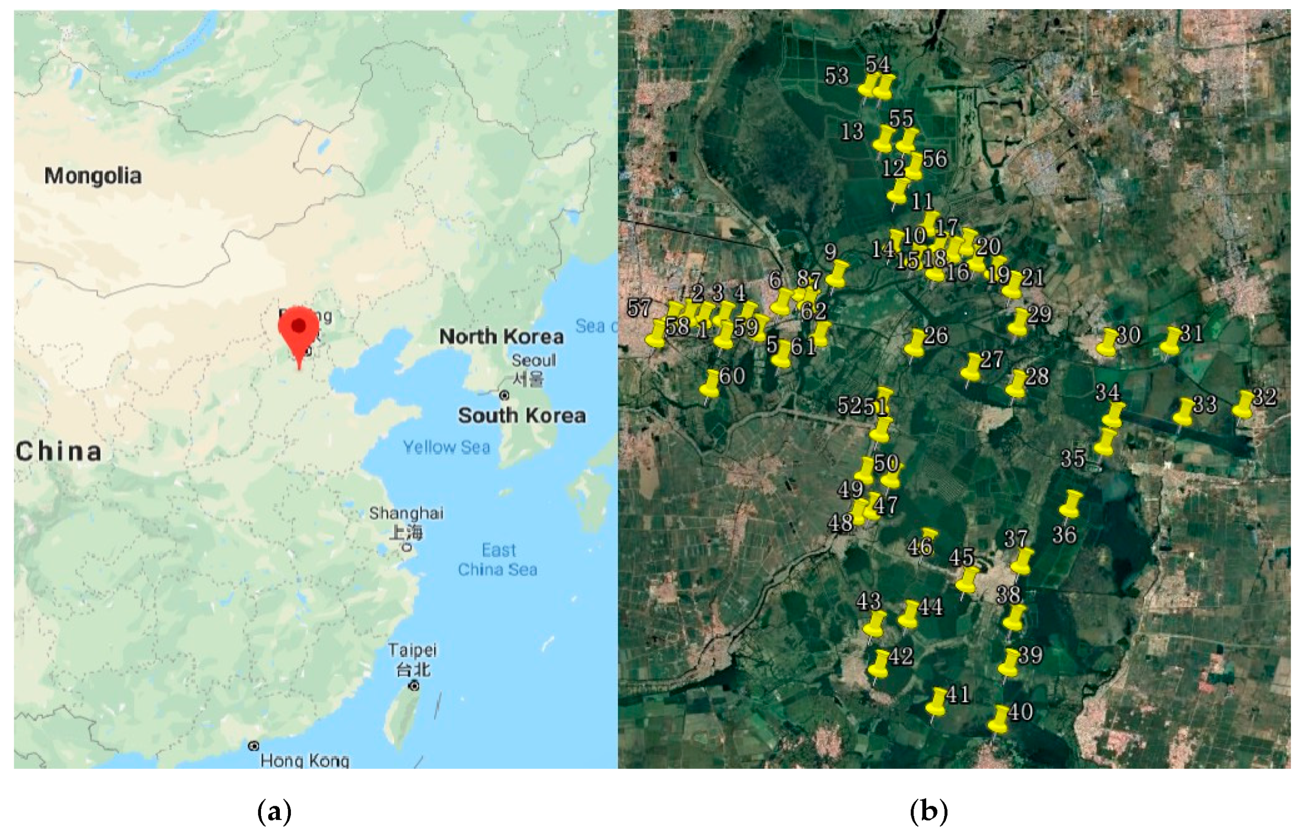
A total of 62 samples were collected from Baiyangdian area. The locations are given in Figure 3. The sampling locations were carefully chosen, given that the main goal of this paper focused on the relationship between the COD value and the hyperspectral data. The authors also wanted to study the impact of human activities on water pollution. Hence, some samples were chosen at the river crossing the city, the edge of the city or the intersection of the rivers. By observing and analyzing the water quality on these points, the information can be acquired on how the human activities impact the water quality. The COD values of all samples were acquired in the laboratory based on conventional chemical methods. These values were treated as the true labels.
This study selected 43 samples as training data and the other 19 samples as testing data. The training and testing sets were representative of the entire water sample set in terms of the minimum, maximum, mean and standard deviation values. This was crucial to our analysis because min-max normalization was used to preprocess the data. This requires similar maxima and minima between the training and testing sets. The statistics of the COD index are given in Table 2. While histograms representing these data are shown in Figure 2.
2.2. The Architecture of Capsule Networks
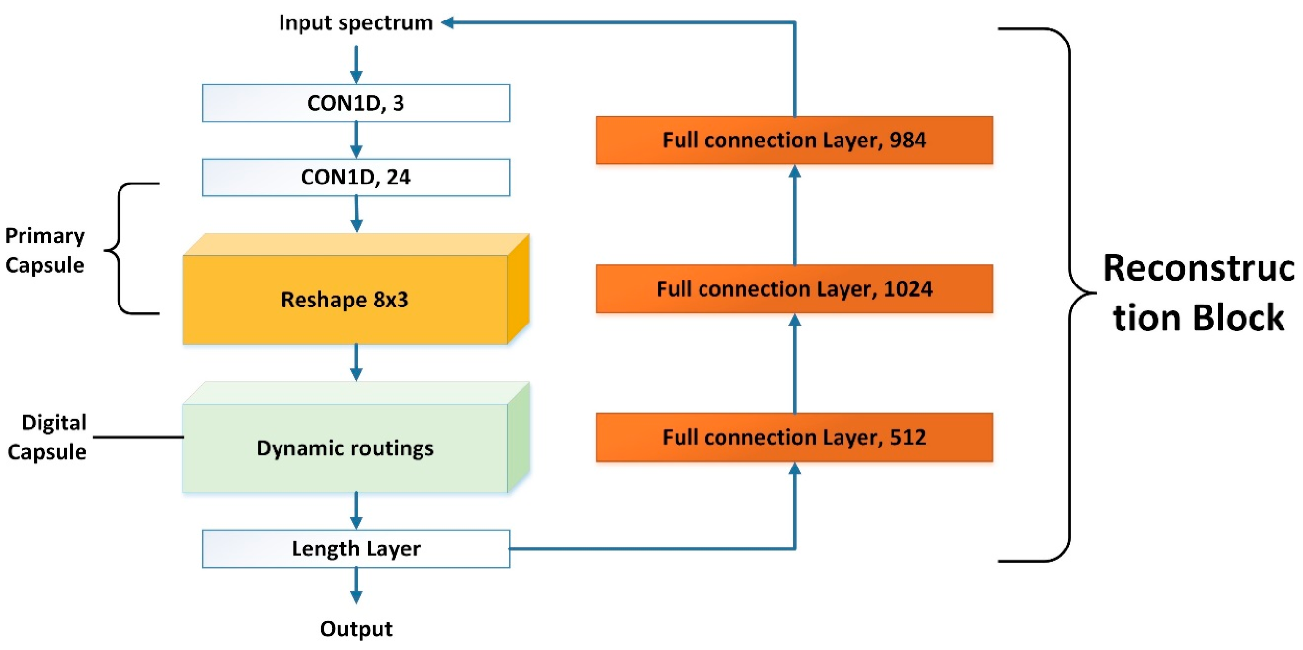
Figure 4 shows the architecture of the capsule network, designed for COD estimation. The model needed to handle 1-D hyperspectral data with a vector length of 984. There are three layers in capsule networks. Each layer was modified to suit our objective. In the first layer, the original 2-D convolution kernel was replaced by a 1-D convolution kernel to fit the 1-D input data. The model was extended by one channel dimension so that the input data met the requirement of the CONV1D function in Python. Moreover, it was found that a small kernel produced better accuracy than a larger one. Hence, a kernel with a size of one was used in our model instead of a kernel of 9 × 9, and only 3 channels were used in our first layer to replace the 256 channels in the original model. It was demonstrated that these modifications reduced the parameters without a loss of accuracy.
The second layer is called the primary capsule layer. In this layer, the capsule dimension of the input was extended. One fast and convenient way to manipulate the method was to apply the convolution kernels to the input and then reshape the output to the designated number of dimensions. For example, in our model, 24 1-D convolution kernels were applied to the input and then reshaped the output to 3 × 8, reflecting 3 channels and an 8-unit length capsule vector. A small kernel size was used with fewer vectors in the capsule dimension compared with the original network.
The third layer is called the digit capsule layer, which is the key part of the capsule network. For all but the first part of the digit capsule layer, the total input to a capsule a weighted sum over-all and is produced by multiplying the output of a capsule by a weight matrix :
where cij are the coupling coefficients determined by the iterative dynamic routing process. The formula for these cij is given by:
where bij is initially set to zero and upgraded by bij = bij + uj|i · vj. In this case, vj is determined in ach iteration in a dynamic routing process. The length of the output vector represents the probability that the entity is contained and exists in the input data. To represent such properties, a non-linear “squashing” activation function, shown in Equation (3) is introduced, which ensures that the short vectors are shrunk to near zero and long vectors are shrunk close to one, leaving their orientation unchanged.
The total routing algorithm is given in Table 3.
The most important aspect of this routing procedure is that it uses dynamic routing to update the weights ci instead of using back-propagation.
The original model had to be modified because the range of the output in the digit capsule layer was not compatible with the label. The original model is supposed to output a probability that is used for classification, which has a range from zero to one. However, this study is dealing with a regression problem. In this case, the true label does not have a constraint on its range. Here, two options were outlined to solve this problem. Either a full-connection layer can be added after the digit capsule layer, whereby this full-connection layer builds a mapping between [0, 1] → R that makes the regression possible, or a min-max normalization can be applied to the label to compress the label into the range [0, 1]. The min-max normalization is preferred because the default weight setting is usually near to zero. In this case, the value of y = ∑ wx + b is small compared with the true label. When the label value is large, then it takes much more time to converge using a full-connection layer. However, there is no such problem, when the label compresses into [0, 1], which has the same range as the output from the digit capsule layer.
Finally, the reconstruction block in the original capsule network was redesigned as a linear regression model for COD quantification, based on the output vector from the digital capsule layer. The reconstruction loss was used to encourage the digital capsule to encode and decode instantiation parameters. During the training, the output of the digital capsule layer was fed into the decoder, consisting of three fully connected layers, as shown in Figure 4.
3. Experiments and Results
3.1. Model for Comparison
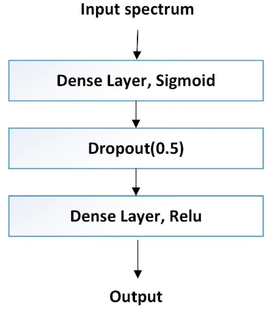
To date, the COD estimation based on remote sensing has been unsatisfactory. Typically, it is based on a partial least square regression (PLSR) or back-propagation algorithm (BP). Therefore, these methods were used for comparison. The parameters for each model were carefully adjusted to achieve the best results for each method. For the PLSR model, 25 components were retained in the model. In the BP algorithm, there were five layers, including one input layer, one output layer, two hidden layers and one dropout layer. The dropout layer is a technique used to improve over-fit on neural networks. The architecture of the BP algorithm is shown in Figure 5.
The COD estimation problem was studied for a while and the result was not satisfactory before the Capsule model was applied. The partial least square regression (PLSR) and back propagation algorithm (BP) were originally used for this problem, and now they were used for comparison purpose. The parameters for each model were carefully adjusted in order to achieve the best result. For the PLSR model, 25 components were retained in the model. For the BP algorithms, there were total five layers, including one input, one output and two hidden layers and one dropout layer. The dropout layer is a technique used to improve over-fit on neural networks. The architecture of the BP algorithms is given in Figure 5.
3.2. Evaluation Criteria and Result
The data set was divided into training and testing sets. The coefficient of determination R2 was used to evaluate the performance of our model. To illustrate the effectiveness of our model, the convergence of the proposed network architecture was evaluated. In this model, it is important to note that the proposed network architecture makes use of several innovative layers that can estimate the probability of the corresponding instantiation parameters. For example, the potential transformations suffered by the corresponding constituent feature on the observable input data. As a result, the features can be intrinsically managed at a higher abstraction level throughout the network. In this context, the plot of the loss function was provided as well as the value of R2 in each epoch. The training procedure did not stop until it reached the predetermined number of iterations. Unless there is an early termination to the procedure, the predicted value of the COD can be obtained in each epoch at the same time the R2 is computed using Equation (4).
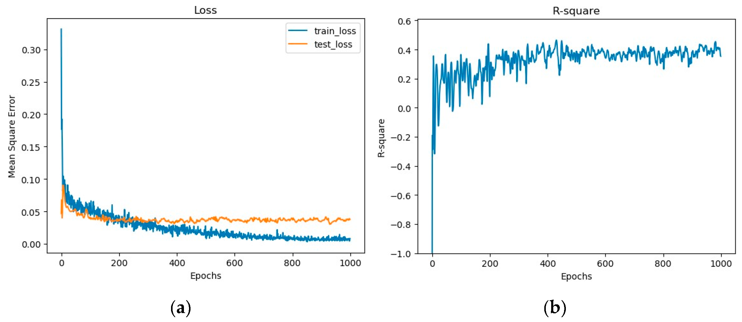
Clearly, the proposed capsule network only requires a reduced number of epochs to reach R2 = 0.7, which highlights remarkably the fast convergence and high accuracy of the proposed architecture compared with the conventional BP algorithm (Figure 6 and Figure 7).
In Figure 7, the final R2 value was 0.78 for the capsule network, while it was only 0.42 for the BP algorithm. For the PLSR algorithm, the R2 was only 0.29 (not shown). All the R2 and mean square error values (MSE) are given in Table 4. Moreover, both predicted and label values are given in Figure 8.
3.3. Parameters Selection
Compared with the original model [23], there are major differences in the parameters chosen for our regression problem. The parameters have been adjusted to provide the best performance of our model as well as a fast convergence time. For instance, there are only three channels in the primary capsule layer and a conv1D layer instead of the 32 and 256 channels of the original model. The following table demonstrates the selection of parameters used to achieve the best performance of our model.
In Table 5, the first number in the channel pair indicates the number of channels in the Conv1D layer and the second number is the number of channels in the primary capsule layer. The program is run on I-5 7400 CPU, so the elapsed time is only valid for the given testing computer. It is shown here for comparison only. Moreover, this study also found that a large kernel was not necessary for our problem. The kernel in the original paper was 9 × 9. A kernel of size 1 was only used. In our experiments, kernels with different sizes were tested. The results are given in Table 6.
In Table 6, the first element in the pair is the kernel used for the conv1D layer and the second element is the kernel used for the primary capsule layer. The best R2 was listed for each experiment. Surprisingly, a large size kernel lowered the accuracy of our results. In the above experiments, a selection of small channels and kernels achieved the best performance. Certainly, a lower number of parameters also lowered the computation time. A similar result was obtained for the BP algorithm, although the more neural did not have higher accuracy and suffered from lower model efficiency as a 1-D regression problem. The reason for this phenomenon is not yet understood.
3.4. Comparison of Denoising Model
In Figure 9, the left panel shows the spectral peaks near 1400 nm, 1900 nm and 2500 nm, caused by water absorption, while the right panel shows the spectra after removing these bands. Here, the results of these two spectra were compared.
In the research of hyperspectral studies, bands selection can help improve prediction ability and reduce model complexity [25,26]. For instance, Levenberg-Marquardt back propagation (LMBP) computes the inverse of the Jacobian matrix of the gradient [27] and the normal Bayes classifier needs to compute the inverse matrix of the covariance matrix. The computation of the inverse matrix occupies a large amount of the computation resource and the reduction on the input bands will largely lower the time consumption. The algorithms involving the computation of the inverse matrix or covariance matrix are sensitive to the input dimension and removing those noising bands is time efficient. Moreover, since the mechanism behinds those bands are clear, the accuracy is usually improved if they are abandoned.
In contrast, our results shown in Table 7 indicate that there is no improvement of accuracy when such noisy bands are removed. The only advantage was that it slightly reduced the computation time because the input dimension had been reduced. Professional researchers often select bands based on different mechanisms, which limits the applications of the data. In our capsule network method, this study demonstrated that it is not necessary to remove these bands. In fact, the network automatically lowers the weights if they do not contribute to the estimation. Our algorithm is easy to implement on any device and does not require any band selection procedure.
4. Conclusions
The capsule network is a recently proposed deep learning network, and only limited studies have explored its potential applications. Motivated by the novelty of the capsule network, this study attempted to use it for hyperspectral regression. Herein, a modified three-layer capsule network for water COD prediction based on 1-D hyperspectral data was provided. It was tested using a real dataset collected in the Baiyangdian area in North China. In addition, a comparable BP network architecture was designed to compare with the capsule network. The capsule network achieved better results, with a limited training set of samples. Moreover, the architecture of the original capsule network was largely simplified because the authors found it unnecessary to use many channels and large kernels. It was also demonstrated that denoising is not necessary for our model, making the model more universally applicable. To the authors’ knowledge, the complexity of the capsule network has not been well explored, and further efforts should be devoted to investigating its potential. The fact that this simple capsule network gave unparalleled performance in COD prediction is an early indication that this method is very useful for 1-D regression problems.
Author Contributions
Conceptualization, C.D. and L.Z.; methodology, C.D.; software, C.D.; validation, C.D.; formal analysis, C.D.; investigation, C.D.; data curation, C.D.; writing—original draft preparation, C.D.; writing—L.Z. and Y.C.; visualization, C.D.; supervision, L.Z.; project administration, L.Z.
Funding
This work was supported by the National Natural Science Foundation of China (No.41830108).
Acknowledgments
We thank Yao Chen, Jiao Wang, Senlin Tang for their effort on the collection of water samples in Baiyangdian area. We thank Trudi Semeniuk from Liwen Bianji, Edanz Editing China for Editing the English text of a draft of this manuscript.
Conflicts of Interest
The authors declare no conflict of interest.
References
- Wei, C.; Wu, H.; Kong, Q.; Wei, J.; Feng, C.; Qiu, G.; Wei, C.; Li, F. Residual chemical oxygen demand (COD) fractionation in bio-treated coking wastewater integrating solution property characterization. J. Environ. Manag. 2019, 246, 324–333. [Google Scholar] [CrossRef] [PubMed]
- Senila, M.; Levei, E.; Cadar, O.; Senila, L.R.; Roman, M.; Puskas, F.; Sima, M. Assessment of availability and human health risk posed by arsenic contaminated well waters from Timis-Bega area, Romania. J. Anal. Methods Chem. 2017, 2017, 3037651. [Google Scholar] [CrossRef] [PubMed]
- Hussain, S.; Shaikh, S.; Farooqui, M. COD reduction of waste water streams of active pharmaceutical ingredient-Atenolol manufacturing unit by advanced oxidation-Fenton process. J. Saudi Chem. Soc. 2013, 17, 199–202. [Google Scholar] [CrossRef]
- Jun, W.; Qi, T.; Junfeng, C.; Fuqiang, Z.; Qiuju, W. Analysis of potassium dichromate method for determining COD in water. Henan Sci. 2012, 9, 1217–1219. [Google Scholar]
- Guo-bing, L. A review on detection methods of chemical oxygen demand in water bodies. Rock Min. Anal. 2013, 6, 860–874. [Google Scholar]
- Liu, F.; Zheng, P.; Huang, B.; Zhao, X.; Jiao, L.; Dong, D. A review on optical measurement method of chemical oxygen demand in water bodies. In Proceedings of the International Conference on Computer and Computing Technologies in Agriculture (CCTA), Beijing, China, 27–30 September 2015; pp. 619–636. [Google Scholar]
- Cuesta, A.; Todolı́, J.L.; Mora, J.; Canals, A. Rapid determination of chemical oxygen demand by a semi-automated method based on microwave sample digestion, chromium (VI) organic solvent extraction and flame atomic absorption spectrometry. Anal. Chim. Acta 1998, 372, 399–409. [Google Scholar] [CrossRef]
- Haiyan, S.; Haiyan, C.; Xiafang, Y.; Yidan, B.; Min, H.; Yong, H. Approach to rapid detection of chemical oxygen demand in livestock wastewater based on spectroscopy technology. 2006. Available online: http://en.cnki.com.cn/Article_en/CJFDTotal-NYGU200606030.htm (accessed on 29 October 2019).
- Ji, Q.; Pan, T.; Liao, X.Y. Rapid Determination of Wastewater COD for Sugar Refinery by TIR/ATR Spectroscopy. J. Jiamusi Univ. Nat. Sci. Ed. 2011, 3, 12. [Google Scholar]
- Jiang, R.; Zhang, C. A dual-wavelength spectroscopic method for the low chemical oxygen demand determination. Spectrosc. Spectr. Anal. 2011, 31, 2007–2010. [Google Scholar]
- Feng, W.W.; Li, L.W.; Li, W.R.; Sun, X.Y.; Fu, L.W.; Zhao, G.L.; Lu, Y.; Zhang, W.; Chen, L.X. On-line monitoring technology for chemical oxygen demand based on full-spectrum analysis. Acta Photonica Sin. 2012, 41, 883–887. [Google Scholar] [CrossRef]
- Alparslan, E.; Coskun, H.G.; Alganci, U. Water quality determination of Küçükçekmece Lake, Turkey by using multispectral satellite data. Sci. World J. 2009, 9, 1215–1229. [Google Scholar] [CrossRef] [PubMed]
- He, W.; Chen, S.; Liu, X.; Chen, J. Water quality monitoring in a slightly-polluted inland water body through remote sensing—Case study of the Guanting Reservoir in Beijing, China. Front. Environ. Sci. Eng. China 2008, 2, 163–171. [Google Scholar] [CrossRef]
- Huang, M.; Xing, X.; Qi, X.; Yu, W.; Zhang, Y. Identification mode of chemical oxygen demand in water based on remotely sensing technique and its application. In Proceedings of the 2007 IEEE International Geoscience and Remote Sensing Symposium (IGARSS), Barcelona, Spain, 23–28 July 2007; pp. 1738–1741. [Google Scholar]
- Qiu, Y.; Zhang, H.E.; Tong, X.; Zhang, Y.; Zhao, J. Monitoring the water quality of water resources reservation area in upper region of Huangpu River using remote sensing. In Proceedings of the 2006 IEEE International Symposium on Geoscience and Remote Sensing (IGARSS), Denver, CO, USA, 31 July–4 August 2006; pp. 1082–1085. [Google Scholar]
- Whistler, J. A phenological approach to land cover characterization using Landsat MSS data for analysis of nonpoint source pollution. KARS Rep. 1996, 96, 1–59. [Google Scholar]
- Eldin, M.S.; Gaber, A.; Koch, M.; Ahmed, R.S.; Bahgat, I. Remote Sensing Application for Water Quality Assessment in Lake Timsah, Suez Canal, Egypt. J. Remote Sens. Technol. 2013, 1, 61–74. [Google Scholar]
- Somvanshi, S.; Kunwar, P.; Singh, N.B.; Shukla, S.P.; Pathak, V. Integrated remote sensing and GIS approach or water quality analysis of Gomti river, Uttar Pradesh. Int. J. Environ. Sci. 2012, 3, 62. [Google Scholar]
- Tehrani, N.; D’Sa, E.; Osburn, C.; Bianchi, T.; Schaeffer, B. Chromophoric dissolved organic matter and dissolved organic carbon from sea-viewing wide field-of-view sensor (SeaWiFS), Moderate Resolution Imaging Spectroradiometer (MODIS) and MERIS Sensors: Case study for the Northern Gulf of Mexico. Remote Sens. 2013, 5, 1439–1464. [Google Scholar] [CrossRef]
- He, B.; Oki, K.; Wang, Y.; Oki, T. Using remotely sensed imagery to estimate potential annual pollutant loads in river basins. Water Sci. Technol. 2009, 60, 2009–2015. [Google Scholar] [CrossRef] [PubMed]
- Chen, Q.; Zhang, Y.; Hallikainen, M. Water quality monitoring using remote sensing in support of the EU water framework directive (WFD): A case study in the Gulf of Finland. Environ. Monit. Assess. 2007, 124, 157–166. [Google Scholar] [CrossRef] [PubMed]
- Ramasamy, S.; Venkatasubramanian, V.; Sam, K.; Chandrasekhar, G.; Ramasamy, S. Remote sensing in pollution monitoring in Cauvery River. In Remote Sensing in Water Resources; Chapter: Chapter 3; Rawat Publications: New Delhi, India, 2005. [Google Scholar]
- Sabour, S.; Frosst, N.; Hinton, G.E. Dynamic routing between capsules. In Advances in Neural Information Processing Systems (NIPS); Neural Information Processing Systems Foundation, Inc.: Montreal, QC, Canada, 2017; pp. 3856–3866. [Google Scholar]
- Willis, C.J. Hyperspectral image classification with limited training data samples using feature subspaces. In Algorithms and Technologies for Multispectral, Hyperspectral, and Ultraspectral Imagery X; The International Society for Optical Engineering (SPIE): Bellingham, WA, USA, 2004. [Google Scholar]
- Keshava, N. Best bands selection for detection in hyperspectral processing. In Proceedings of the 2001 IEEE International Conference on Acoustics, Speech, and Signal Processing. Proceedings (Cat. No. 01CH37221), Salt Lake City, UT, USA, 7–11 May 2001; Volume 5, pp. 3149–3152. [Google Scholar]
- Sun, W.; Zhang, X.; Sun, X.; Sun, Y.; Cen, Y. Predicting nickel concentration in soil using reflectance spectroscopy associated with organic matter and clay minerals. Geoderma 2018, 327, 25–35. [Google Scholar] [CrossRef]
- Yu, H.; Wilamowski, B.M. Levenberg-marquardt training. Ind. Electron. Handb. 2011, 5, 1. [Google Scholar]
Figure 1.
An example the capsule networks ability to carry out segmentation of highly overlapping digits in the Modified National Institute of Standards and Technology (MNIST) dataset [23].
Figure 1.
An example the capsule networks ability to carry out segmentation of highly overlapping digits in the Modified National Institute of Standards and Technology (MNIST) dataset [23].

Figure 2.
(a) Hyperspectral plot for Baiyangdian area; and (b) chemical oxygen demand (COD) distribution based on samples from Baiyangdian area.
Figure 2.
(a) Hyperspectral plot for Baiyangdian area; and (b) chemical oxygen demand (COD) distribution based on samples from Baiyangdian area.

Figure 3.
(a) Location of Baiyangdian area in North China; and (b) Locations of water samples at Baiyangdian area.
Figure 3.
(a) Location of Baiyangdian area in North China; and (b) Locations of water samples at Baiyangdian area.

Figure 4.
Schematic showing the capsule network architecture and the modifications used in this study.
Figure 4.
Schematic showing the capsule network architecture and the modifications used in this study.

Figure 5.
Schematic showing the back-propagation algorithm architecture used for comparison in this study. It consists of one input layer, one output layer, two hidden layers and one dropout layer.
Figure 5.
Schematic showing the back-propagation algorithm architecture used for comparison in this study. It consists of one input layer, one output layer, two hidden layers and one dropout layer.

Figure 6.
(a) Loss plot and (b) coefficient of determination (R-square) values for the back-propagation algorithm.
Figure 6.
(a) Loss plot and (b) coefficient of determination (R-square) values for the back-propagation algorithm.

Figure 7.
(a) Loss plot and (b) coefficient of determination (R-square) values for the capsule network method.
Figure 7.
(a) Loss plot and (b) coefficient of determination (R-square) values for the capsule network method.

Figure 8.
Chemical oxygen demand (COD) prediction by capsule model.

Figure 9.
(a) Original spectra and (b) Denoised spectra used as inputs to the capsule network model in this study.
Figure 9.
(a) Original spectra and (b) Denoised spectra used as inputs to the capsule network model in this study.


Table 1.
Literature review of the estimation of physicochemical parameters of water using a remote sensor.
Table 1.
Literature review of the estimation of physicochemical parameters of water using a remote sensor.
| Sensor | Reference |
|---|---|
| Landsat 5-TM | [12,13,14,15] |
| Landsat 5-MSS | [16] |
| WorldView-2 | [17] |
| IRS-LISS-III | [18] |
| MODIS | [19] |
| MERIS | [19] |
| AVHRR | [20] |
| SeaWiFS | [21] |
| SPOT | [22] |
Table 2.
Statistical information for the chemical oxygen demand (COD) index for the study area.
| Group | Min | Max | Mean | Median | SD |
|---|---|---|---|---|---|
| Training set | 10 | 27 | 17.26 | 17 | 4.49 |
| Testing set | 13 | 26 | 18.68 | 19 | 3.85 |
| Entire dataset | 10 | 27 | 17.69 | 17 | 4.36 |
Table 3.
Dynamic Routing Procedure.
| For r Iterations Do | |
|---|---|
| 1: | ci = so f tmax(bi) |
| 2: | |
| 3: | vj = squash(sj) |
| 4: | |
| 5: | Return vj |
Table 4.
Coefficient of determination (R2) and mean square error (MSE) for the three models: Capsule network, back-propagation algorithm (BP) and partial least square regression (PLSR).
Table 4.
Coefficient of determination (R2) and mean square error (MSE) for the three models: Capsule network, back-propagation algorithm (BP) and partial least square regression (PLSR).
| Test Set | Capsule | BP | PLSR |
|---|---|---|---|
| R2 | 0.7812 | 0.4189 | 0.2941 |
| MSE | 0.0112 | 0.0377 | 0.0416 |
Table 5.
Comparison of channel selection options in our model (coefficient of determination, R2).
| Channel Pair | R2 | Elapsed Time (400 Epochs) |
|---|---|---|
| (3, 3) | 0.7812 | 63.5 s |
| (3, 32) | 0.7812 | 185.5 s |
| (32, 32) | 0.7157 | 212.7 s |
| (32, 64) | 0.7171 | 507.3 s |
| (256, 32) | 0.6169 | 281.0 s |
Table 6.
Comparison of kernel selection options in our model (coefficient of determination, R2) Kernel Selection Comparison.
Table 6.
Comparison of kernel selection options in our model (coefficient of determination, R2) Kernel Selection Comparison.
| Kernel Size Pair | R2 |
|---|---|
| (1 × 1, 1 × 1) | 0.7812 |
| (3 × 3, 3 × 3) | 0.7477 |
| (5 × 5, 5 × 5) | 0.7032 |
| (7 × 7, 7 × 7) | 0.6806 |
Table 7.
Comparison results of removing some bands from the original spectra (coefficient of determination, R2; mean square error, MSE).
Table 7.
Comparison results of removing some bands from the original spectra (coefficient of determination, R2; mean square error, MSE).
| R2 | MSE | |
|---|---|---|
| Original spectrum | 0.7812 | 0.0112 |
| Removing bands near 1400 nm, 1900 nm and 2500 nm | 0.7513 | 0.0128 |
| Removing bands near 1900 nm and 2500 nm | 0.7562 | 0.126 |
| Removing bands near 2500 nm | 0.7528 | 0.0127 |
© 2019 by the authors. Licensee MDPI, Basel, Switzerland. This article is an open access article distributed under the terms and conditions of the Creative Commons Attribution (CC BY) license (http://creativecommons.org/licenses/by/4.0/).
Share and Cite
MDPI and ACS Style
Deng, C.; Zhang, L.; Cen, Y. Retrieval of Chemical Oxygen Demand through Modified Capsule Network Based on Hyperspectral Data. Appl. Sci. 2019, 9, 4620. https://0-doi-org.brum.beds.ac.uk/10.3390/app9214620
AMA Style
Deng C, Zhang L, Cen Y. Retrieval of Chemical Oxygen Demand through Modified Capsule Network Based on Hyperspectral Data. Applied Sciences. 2019; 9(21):4620. https://0-doi-org.brum.beds.ac.uk/10.3390/app9214620
Chicago/Turabian StyleDeng, Chubo, Lifu Zhang, and Yi Cen. 2019. "Retrieval of Chemical Oxygen Demand through Modified Capsule Network Based on Hyperspectral Data" Applied Sciences 9, no. 21: 4620. https://0-doi-org.brum.beds.ac.uk/10.3390/app9214620
Note that from the first issue of 2016, this journal uses article numbers instead of page numbers. See further details here.