Railway Track Monitoring Using Train Measurements: An Experimental Case Study


1
School of Civil Engineering, University College Dublin, D04V1W8 Dublin, Ireland
2
Murphy Surveys, Global House, Kilcullen Business Campus, D04V1W8 Kilcullen, Co. Kildare, Ireland
3
Iarnród Éireann Irish Rail, Technical Department, Engineering and New Works, Inchicore, D01V6V6 Dublin, Ireland
*
Author to whom correspondence should be addressed.
Appl. Sci. 2019, 9(22), 4859; https://0-doi-org.brum.beds.ac.uk/10.3390/app9224859
Submission received: 18 September 2019
/
Revised: 30 October 2019
/
Accepted: 7 November 2019
/
Published: 13 November 2019
(This article belongs to the Section Civil Engineering)
Abstract
:This paper investigates the use of drive-by train measurements for railway track monitoring. An in-service Irish Rail train was instrumented while using accelerometers and a global positioning system. The measurements were taken over two months and the train bogie accelerations from 60 passes on the Dublin-Belfast line were used for this study. A 6 km section of the line is the particular focus, where the maintenance measurements from a Track Recording Vehicle (TRV) were available. The Hilbert transform is used to obtain the instantaneous amplitudes of the acceleration signals. A new representation of the signal is proposed to show the signal energy level as a function of train location. It is shown that the forward speed of the train has a significant influence on the energy level of the signals. Therefore, a two-step speed correction is applied to the data. First, data from passes with forward speed below a certain limit are removed from the data set. Subsequently, a scaling factor is defined for the remaining signals and the energy levels of those signals are scaled while using online speed measurements. The scaled amplitudes are compared with the TRV data. It is shown that the energy levels of the signals match the TRV measurements very well.
1. Introduction
Railways constitute a major portion of transport infrastructure in most countries. It is essential to employ good strategies for the maintenance of railway networks to avoid a disruption to services and ensure the safety of the system. For example, the railway track condition needs to be regularly monitored to detect faults at an early stage before they become major issues. Several types of defect can happen on railway tracks: rail cracks, track settlement, landslides onto track, hanging sleepers, etc. [1]. Visual inspection or ‘walking the track’ is one of the most common methods of track inspection. However, it is expensive, subjective, and some faults can be missed. A track recording vehicle (TRV) is a mechanised method of railway track inspection while using optical and inertial sensors in a specialised vehicle. The inspection vehicle periodically travels over the rail network and measures several geometric parameters of the track, such as: longitudinal level of left and right rail, alignment of left and right rail, track gauge, cross level, twist, curvature and curve radius, gradient, and position using GPS [2]. However, these vehicles are expensive and they may not always be available for the whole network. In addition, they do not always travel at the same speed as normal train traffic, which, in some cases, disrupts regular services.
Drive-by monitoring is an inspection method in which the responses that are measured on instrumented trains/vehicles are employed for the condition monitoring of components of transport infrastructure, e.g., bridges [3,4], highway pavements [5], and railway tracks [6,7]. In the railway application, sensors are installed on an operational train to provide faster, cheaper, and more reliable monitoring approaches. It does not disrupt service provision and it can provide real time data on track condition, facilitating more timely responses to developing track failures. Such instrumentation can obviate the need for specialist vehicles, such as the TRV. In effect, it is a move from a small number of accurate measurements under controlled conditions to a large number of less accurate and less controlled measurements.
Several types of sensor technology have been employed for drive-by railway track monitoring, such as: laser technology [8], camera [9,10], and inertial sensors (accelerometers, gyrometers, etc.) [11]. Some of these technologies can be used together or separately, depending on the main purpose of monitoring. Laser optical sensors are usually considered to be expensive and they may involve a high maintenance cost. Camera-based systems are cheaper to be employed, but they require expensive image processing methods and provide limited information. Inertial sensors have been extensively used in the literature due to their simplicity, low price, and effectiveness. Inertial sensors can be installed on the train axle box, bogie, or inside the carriage, and the responses are continuously measured. These measurements have been used for several health monitoring purposes in the literature, as summarized in Table 1.
In the context of railway track components, Wei et al. [13] investigate the degradation of a railway crossing while using real train axle box measurements over time. They show that uneven deformation between the wing rail and crossing nose and local irregularity in the longitudinal slope of the crossing nose can be identified. Oregui et al. [14] employ axle box acceleration measurements for the monitoring of bolt tightness of rail joints. Molodova et al. [15] use drive-by measurements from a train axle box for condition monitoring of insulated joints. The power spectrum of the acceleration signals is used as a damage indicator. Salvador et al. [16] present a surveying approach for the detection and classification of track parameters, such as welded joints, turnout frogs, and squats. Changes in track typologies can be detected using measurements from a train axle box.
Several researchers have proposed using inertial measurements to find the railway track stiffness profile. Quirke et al. [18] propose the use of drive-by measurements to detect railway track stiffness variation while using an optimization algorithm. Although their method provides good accuracy, it is computationally expensive and it has not been confirmed by experimental data. Le Pen et al. [19] use on-train measurements to identify changes in track support stiffness. Real et al. [17] propose a method that uses a Fourier transform to find the rail profile while using vertical accelerations that were measured on a passing train. OBrien et al. [11] employ an inverse technique to find the longitudinal track profile using inertial measurements from an in-service train. The track longitudinal profile that generated the vehicle model responses that best match the measured responses is found using the Cross Entropy optimization technique. Tsunashima et al. [24] develop a portable condition monitoring system for track, which is integrated into an in-service train. In this method, the rail irregularities can be estimated from the vertical and lateral accelerations of the car body. Kobayashi et al. [25] use a Kalman Filter to solve an inverse problem, showing the possibility of only estimating the track irregularities from car-body motions. Paixão et al. [26] present an approach that uses acceleration measurements from smartphones inside in-service trains for the assessment of the structural performance and geometrical degradation of railway tracks. They obtain cross-correlation values of greater than 0.85 between the standard deviations of the longitudinal level and the vertical accelerations measured on-board a passenger train on an 11 km stretch of railway.
Cantero and Basu [20] use wavelet transforms of acceleration responses to a passing train to identify any railway track irregularities. They use a simple model and do not consider track stiffness. Tsai et al. [22] propose the application of the Hilbert transform to the measured signals from the axle box of an operational train. They show that decomposing the signals while using the Hilbert transform has the potential to find track irregularities. Recently, Lederman et al. [23] propose an energy-based approach for track change monitoring. They plot the average energy of the measured acceleration in the space domain in a contour plot. A feature detection method is proposed to find changes in the contour plot, which can be indicators of faults on the track. In another study, Lederman et al. [27] show that in some parts of the track, the train is more excited which creates bumps in the measured acceleration signals. They suggest that changes in the sizes of the bumps in consecutive runs are indicative of changes to the track.
Although energy-based methods have shown good potential for railway track monitoring while using multiple passes, there are several challenges that need to be overcome. The first one is the method of representing the average energy of signals. The current method that was proposed by Lederman et al. [23] estimates the energy by summing the amplitudes of the acceleration signal over a pre-specified window. This method might not be accurate if the window length is not well defined. Another important challenge is the influence of train forward speed to the amplitude of the measured signals. There is usually considerable speed variation in multiple train passes over the same route. This variation has considerable influence on the energy of the signals. For example, a higher forward speed might create a higher energy for the same section of track than a lower speed. Therefore, it is difficult to determine whether the change in the signal energy is due to speed variation or track change. These challenges in the energy-based methods are addressed in this paper.
In this paper, an algorithm is proposed for railway track fault detection while using measurements on the bogie of an in-service train. A regular Irish Rail passenger train was instrumented while using accelerometers and a Global Positioning System (GPS). The location of the train and its approximate forward speed were recorded using the GPS system. Six kilometres of Dublin-Belfast railway line is inspected here from 60 train passes. The instantaneous amplitudes of the acceleration signals are extracted while using the Hilbert transform. A novel process is proposed for finding the energy levels of the amplitudes in the space domain. A data cleaning process is performed to remove the passes with low energy due to low train forward speeds. The cleaned data are then scaled using a new scaling method that emphasizes the importance of the vehicle forward speed to the level of energy. The scaled energy signals show a high level of consistency, which is ideal for the frequent inspection of railway tracks. It is suggested that a consistently high level of scaled energy over multiple passes might indicate a possible defect in the track. The TRV data recorded after the train measurements are used to check the track condition at two areas with high energy levels. It is shown that high energy parts of the track match well with the faults identified in the TRV data.
2. Measurements
2.1. The Instrumented Train
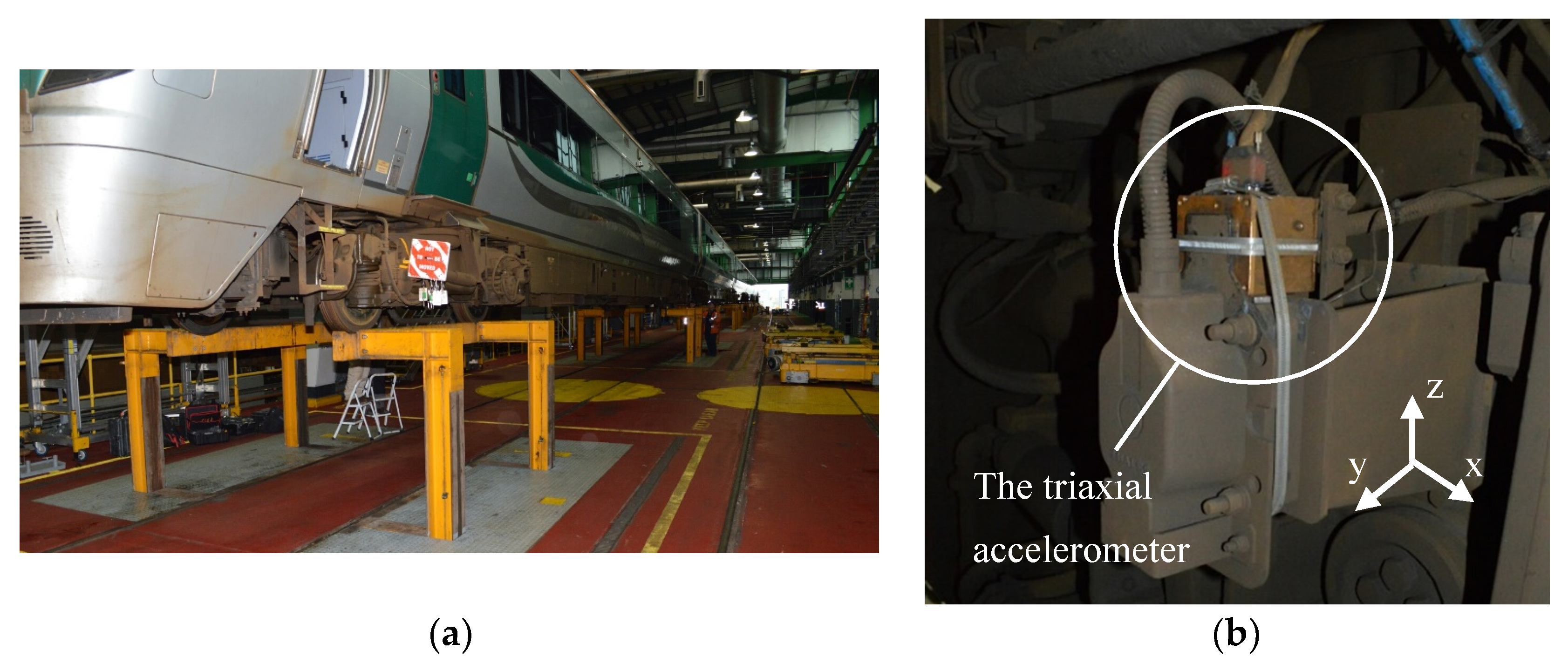
An Irish Rail Hyundai Rotem InterCity fleet car (Figure 1a) was instrumented while using inertial sensors that were installed on the trailer (non-powered) bogie in December 2015. The data was measured on the leading car (22337) of Set 37, a five-car train set. The train was in operation in the Dublin-Belfast Enterprise service line and the measurement equipment was installed while the train was stabled for a routine examination. The sensors were installed on the trailer bogie to minimize the noise contamination from the power train. A tri-axial accelerometer (Disynet-DA3802-015g with a range of ±15 g) and tri-axial gyrometer (Crossbow VG400CC-200 with a range of ±200°/s) (Figure 1b) were installed on the bogie as close as possible to its center of mass. The data were measured at a sampling frequency of 500 Hz. The train location was also recorded while using a GPS antenna. The approximate forward speed of the train was obtained from the GPS data and referenced to its location. The GPS system recorded the train position at a frequency of 5 Hz. The sensors and GPS system were connected to a HBM Somat eDAQ-lite data logger with 32 GB storage capacity to collect and store the data. The data logger was installed at an optimal location on the train which needed minimum cabling. Power was taken from a spare circuit breaker on the underside of the carriage, which meant that the system required no connection into the carriage, satisfying the requirements of Irish Rail. The data were collected on the Dublin-Belfast line from 13 January to 3 February 2016. In total, 57 return journeys were taken on the line during this time. There was insufficient bandwidth to allow for the transfer of the data over a GSM network. Instead, an operator used a secure Wi-Fi connection to download the data from the data logger once every 7–10 days. The Wi-Fi connection avoided the need for physical access to the data logger, which was located underneath the carriage.
2.2. Accelerations
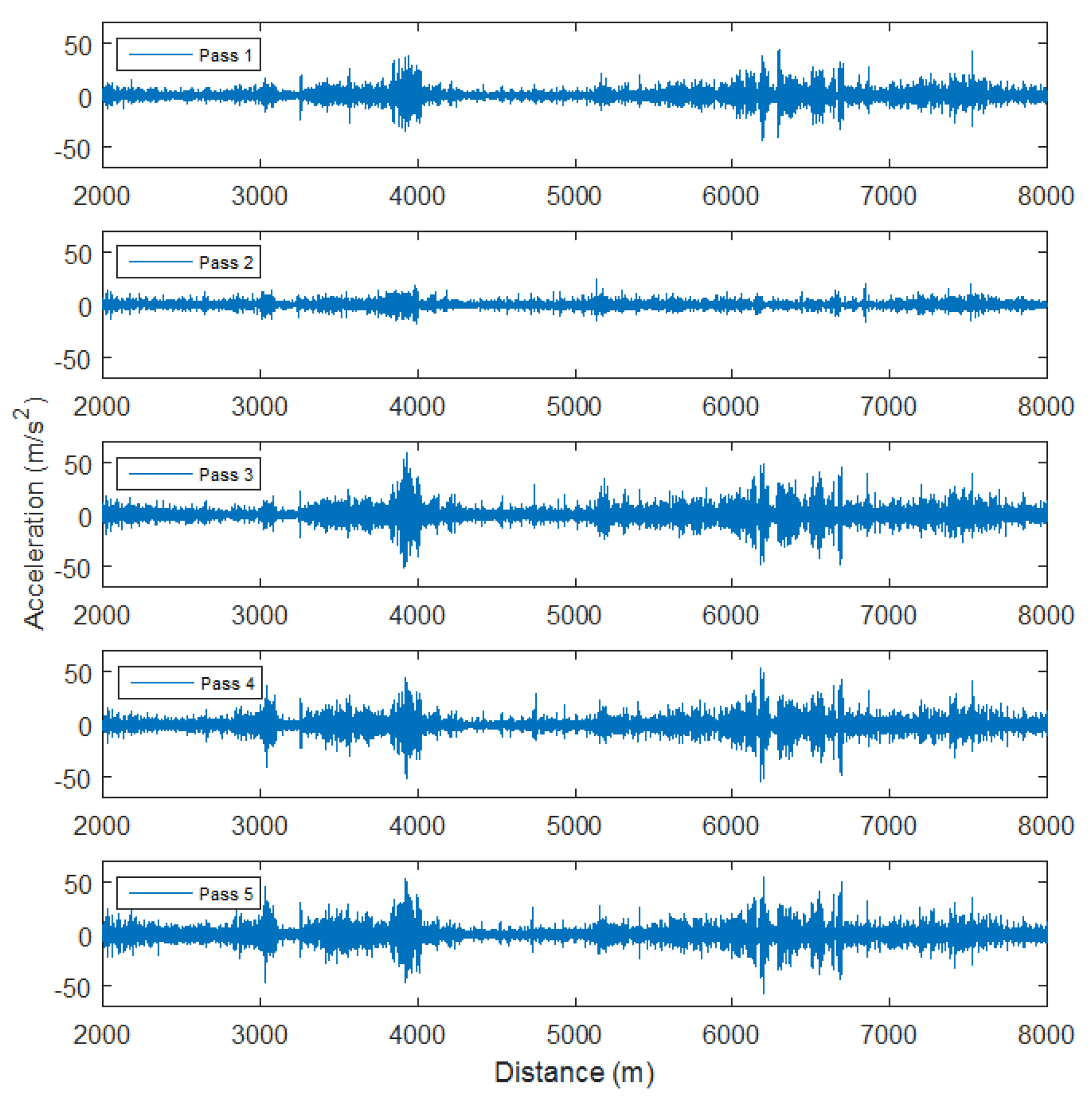
Figure 2 shows the accelerations measured on the first five passes against train location. The train forward speed is assumed constant for each GPS sample and the position of the train has been calculated while using linear interpolation of that data. The amplitude of the accelerations is at different levels as the train moves along the rail. It can be also noticed that, with the exception of the second pass, the patterns are similar, but at different levels. For example, the four signals contain a peak with high amplitude at a distance of around 4000 m. However, Pass 1 has maximum amplitude at this location of 38.15 m/s2, while Pass 3 has amplitude of 59.43 m/s2, which is approximately 1.5 times that of Pass 1. Pass 2, on the other hand, has low levels of amplitude at most of the locations.
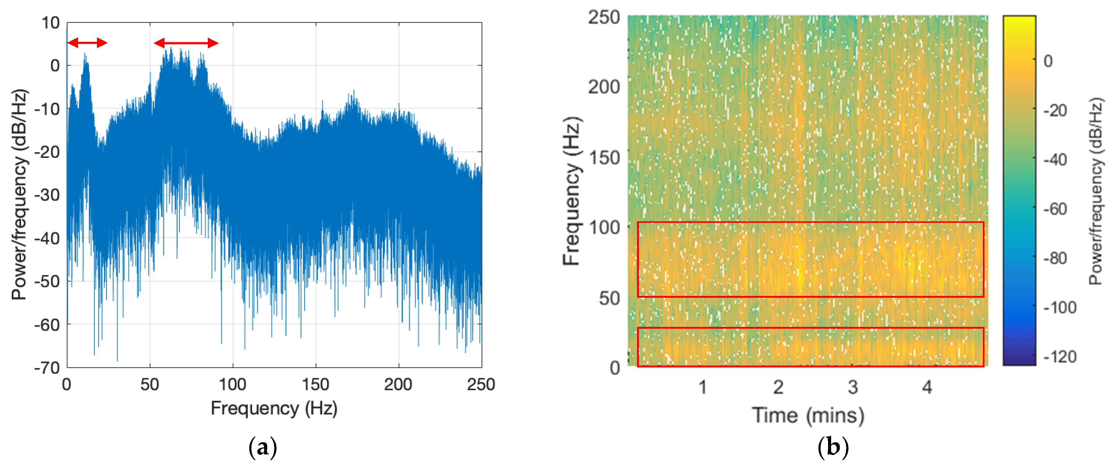
The frequency spectra of the measured signals may provide insights into the data. Figure 3a shows the frequency content of Pass 3 while using a Fast Fourier Transform (FFT). It can be seen that there are two dominant frequency ranges in the signal; under 20 Hz and 60–90 Hz. As the signal is long, measured for about 6 km over a period of about 5 min., FFT has the significant disadvantage of not providing any spatial information. Therefore, a Short Time FFT (STFFT) is employed to show the frequency components of the signal in both the frequency and time (space) domains. The STFFT spectrum in Figure 3b shows that the ranges mentioned above are dominant for most locations as the train moves forward. It can be concluded that the signal components under 100 Hz contribute most of the energy of the signal.
It has been stated in the literature [28,29,30,31] that typical train eigenfrequencies are in the range of 0.5–15 Hz. This suggests that the first frequency range mentioned above is predominately related to vehicle dynamics. It has been shown in [32] that the dominant peaks in the second range are dependent on the vehicle forward velocity and rail surface irregularities. This means that the second frequency range corresponds to properties, such as rail roughness profile and sleeper spacing frequency, which is of most interest in this paper.
3. Energy of Acceleration Signals
As suggested by Lederman et al. [23], the energy of vertical acceleration signals measured on a passing train contains useful and important information regarding the railway track condition. For example, if the train passes over a bump or a defect on the track, the acceleration signal measured on the train might contain high amplitudes that represent high levels of energy at that location. Lederman et al. [23] propose using the average amplitudes of the signal using a moving window along the track. The signal energy in each window is then obtained by summing the amplitudes of the acceleration signal. Here, the signal amplitudes are obtained while using the Hilbert transform. Hence, the energy is represented by the true local peaks of the signal instead of averaging.
3.1. Hilbert Amplitude
The amplitude of the signals is extracted while using the Hilbert transform. This represents the energy of the vertical acceleration signal by extracting its instantaneous amplitude. The Hilbert transform of is [33]:
where presents the Cauchy principal value of the singular integral. The analytic signal of , which is a complex signal is defined by [33]:
where is . The polar form of is:
The instantaneous amplitude is calculated as:
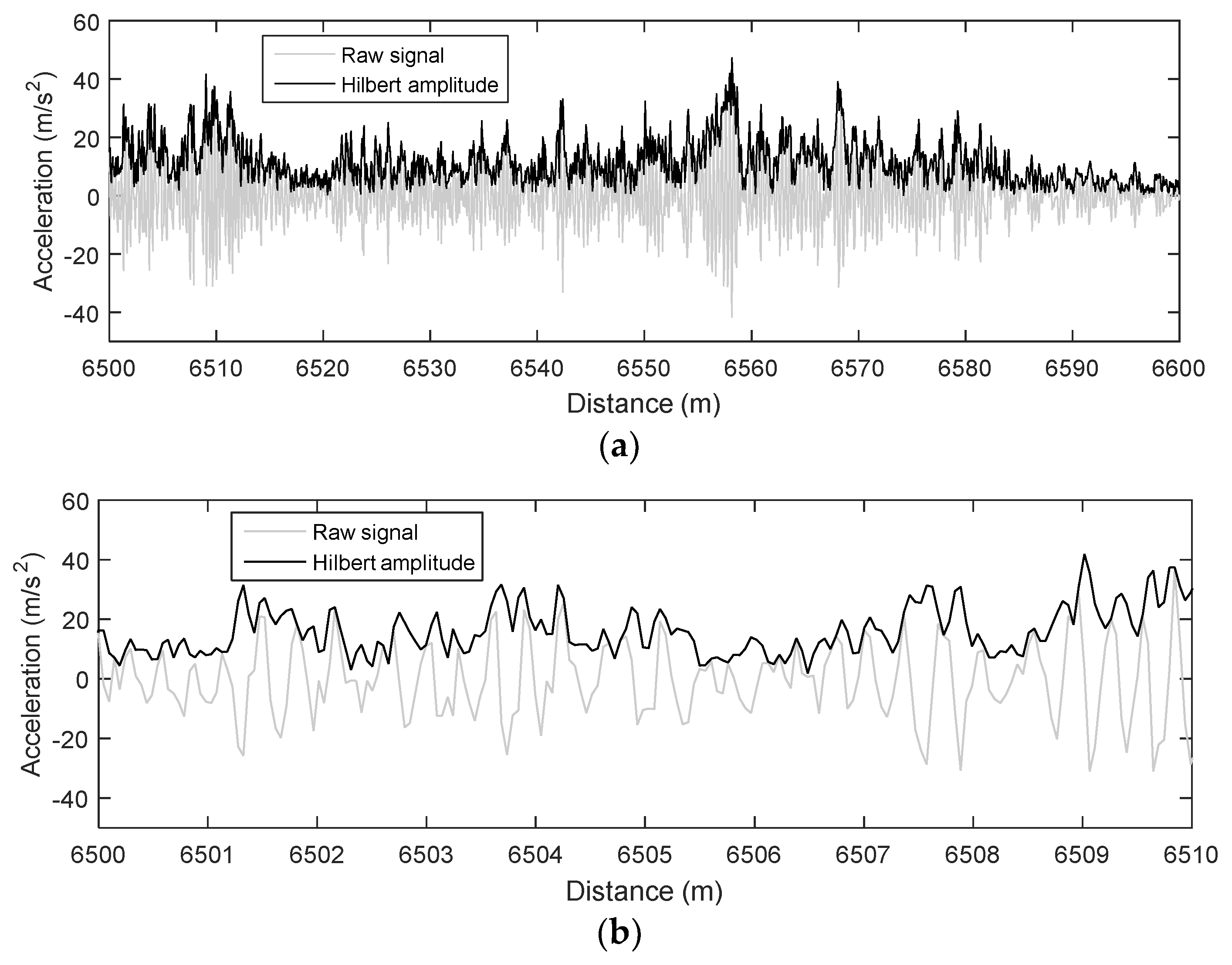
The Hilbert amplitude of a vertical acceleration signal, , as measured over a distance of 300 m from a sample of the data set, is shown in Figure 4. It shows how the Hilbert transform extracts the instantaneous amplitude of the signal, which represents the signal energy.
3.2. Peak Based Decomposition
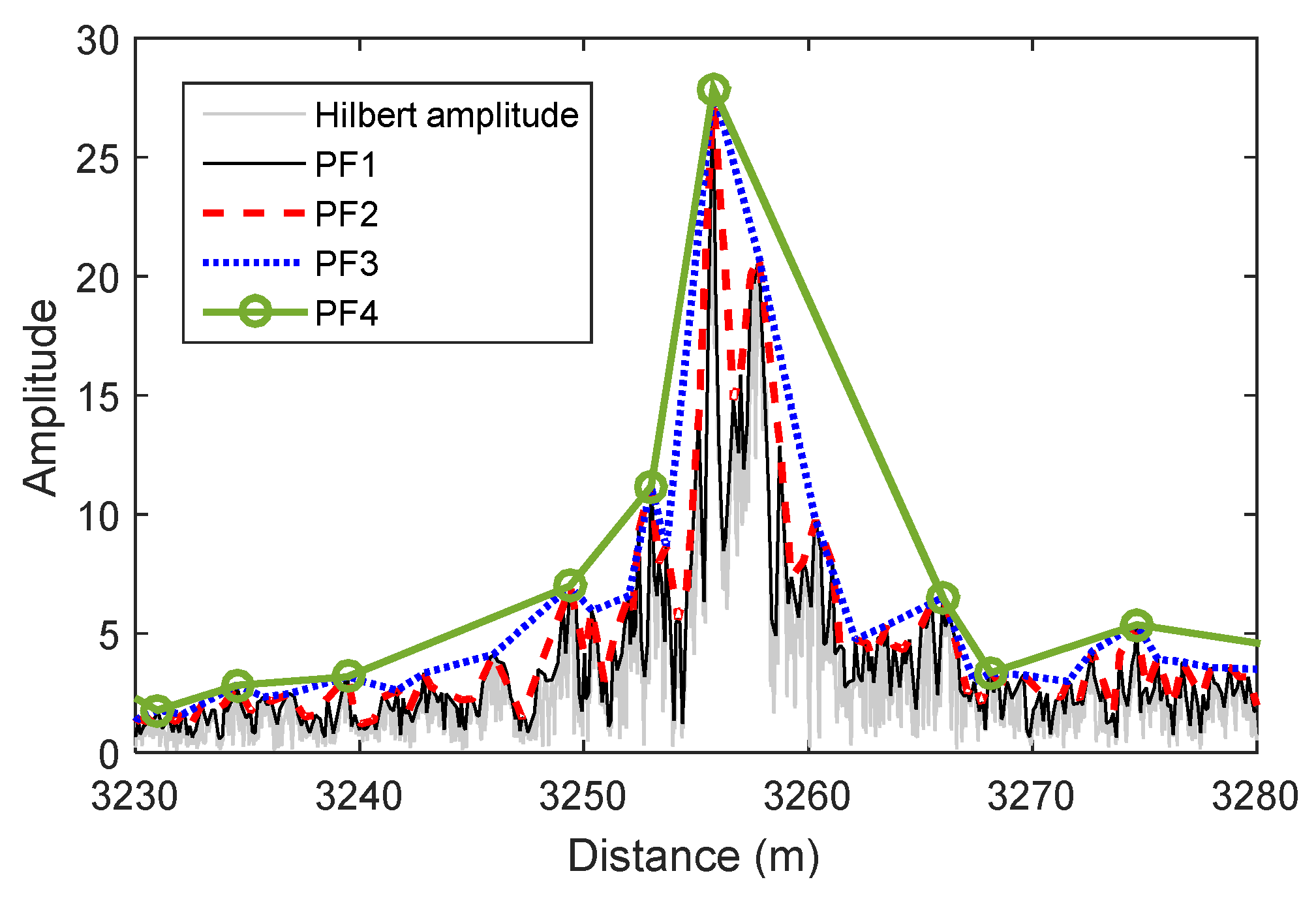
The instantaneous amplitude of a signal is sampled at the same rate as the original signal, which means that they have same length. When the dataset for the entire track length is being processed, it is necessary to reduce the size of the data to avoid time consuming and computationally expensive signal processing. At the same time, the energy information in the signal needs to be retained. In this section, a simple process, called peak based decomposition (PBD), is proposed to represent the signal energy in a much more compact function. PBD employs a simple multi-step process. In each step, the local maxima of the Hilbert amplitudes are taken and stored as a new representation of the same signal. In this way, small peaks in the original amplitude signal are removed, but the main peaks are kept. The output of this process constitutes a shorter length version of the original signal, but it contains the significant energy levels of the signal in the space domain. The output of the first step is called Peak Function 1 (PF1). If the process is repeated on PF1, then a new shorter version of the signal is obtained, which is called PF2. The process can be repeated several times until the desired combination of signal energy and length is obtained. Figure 5 shows how PBD works by approximating the original signal in each step and decomposing it to reduced sizes while the main amplitudes are kept.
The PBD process is applied to a 400 m sample of measurement in Figure 6. It can be observed how PF4 and PF5 represent the energy level of the raw signal. The average signal energy that was proposed by Lederman et al. [23] using a 25 m window is also shown. As this algorithm averages the energy of the signal in a pre-specified window, it might not accurately find the locations in which the signal contains high levels of energy. In addition, if the width of the window is not properly chosen, the algorithm will sort the energy of part of signal into two windows and reduce the real amplitude. This might cause some parts of the signal with high energy levels not to be discovered. Fortunately, there is no need to select a window band with PBD.
Accurately finding the peaks is important when multiple train runs are studied where the alignment of multiple measurements in the space domain is required. The proposed PD process produces a peak at the right location with good accuracy. This allows for the peaks to be aligned from several runs. However, there are several factors contributing to the accuracy of peak locations, e.g., the performance of the GNSS under different train forward speeds. These factors may cause some levels of mismatch between the responses in different passes.
4. Forward Speed of the Train
4.1. Forward Speed
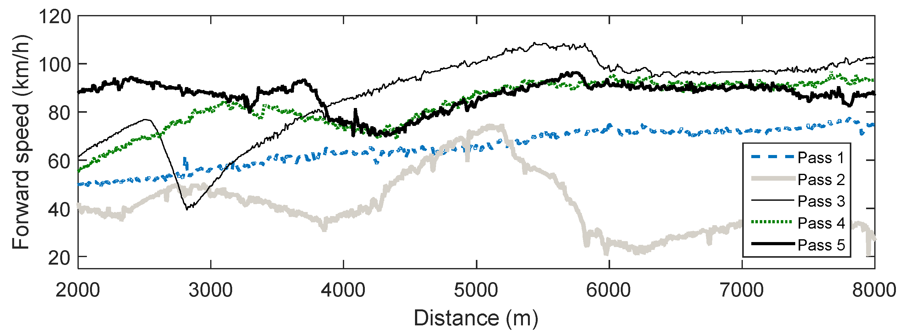
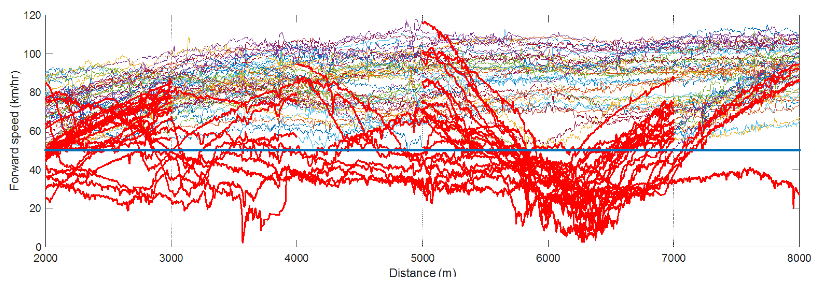
The forward speed of the train has a direct influence on the energy of the signal. For example, if the train passes over a defect with low speed, it might not create enough energy for that defect to be detected. As a result, there may be some passes that show high energy levels at a specific location, but some others with low amplitudes. Figure 7 shows the forward speeds for the first five passes from the dataset. It can be seen that there is considerable speed variation, which is the result of several factors, such as driver behavior, temporary speed restrictions, earlier delays, or weather. The second pass has the lowest speed through most of the sample zone.
Figure 2 shows that, in the second pass, there is a low amplitude between 6000 and 7000 m relative to the other passes in this zone. This amplitude level is not useful in this study. Therefore, a cleaning process was employed to remove the low-speed signals from the dataset. In this work, the forward speed of the train at each kilometer point was monitored and data removed for segments of data for which the minimum speed was less than 50 km/h.
4.2. Energy Scaling Using Forward Speed
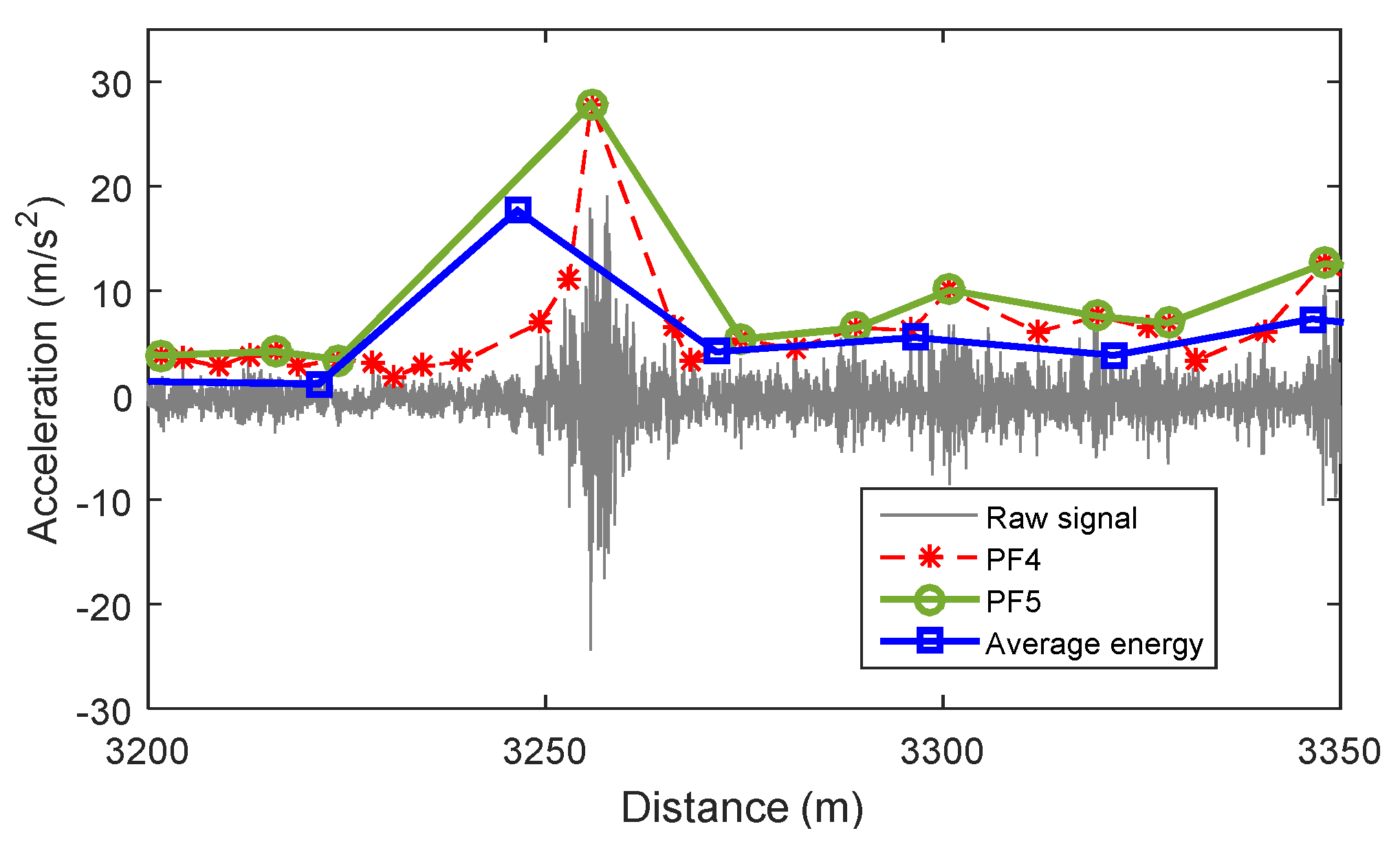
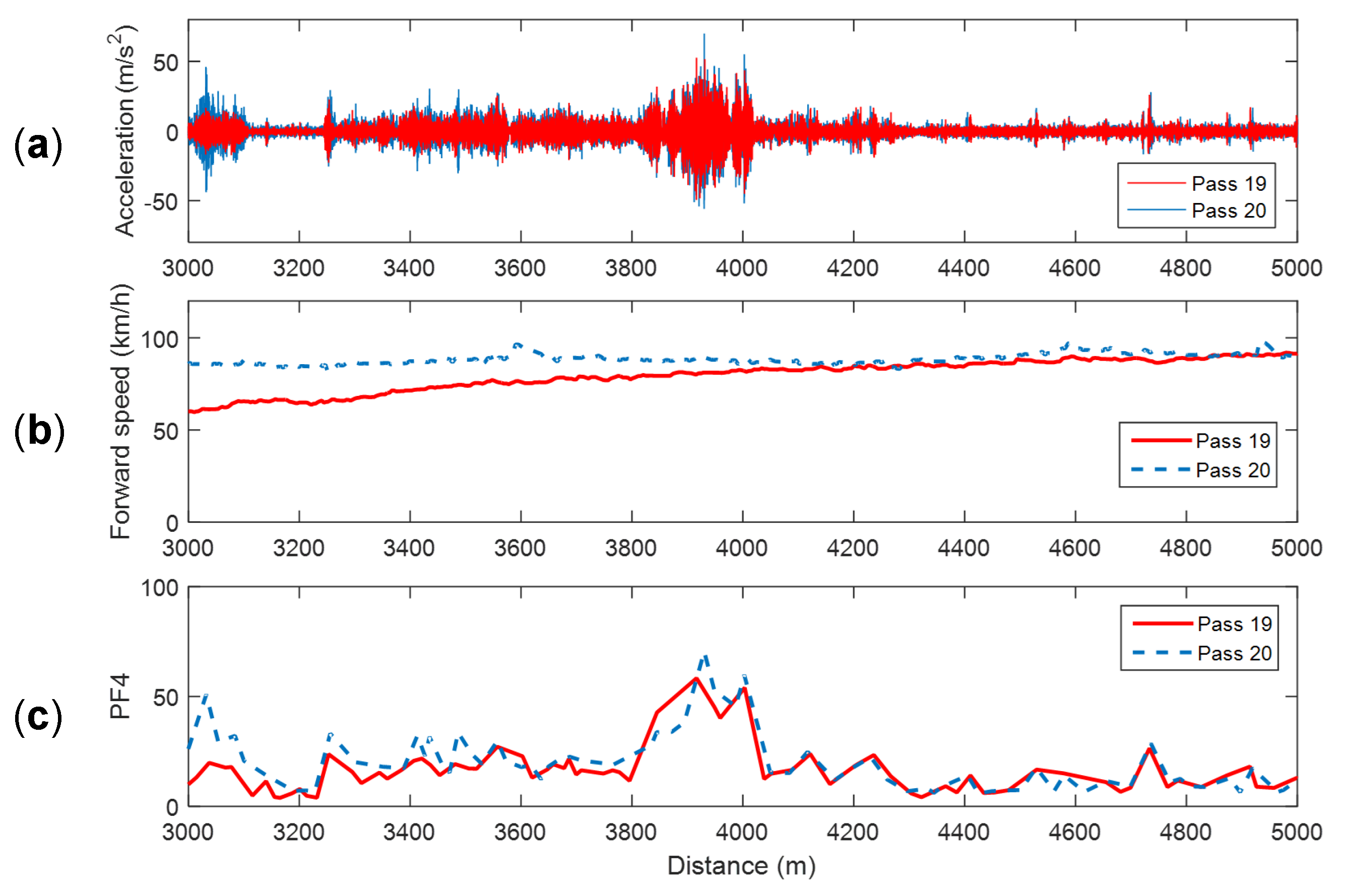
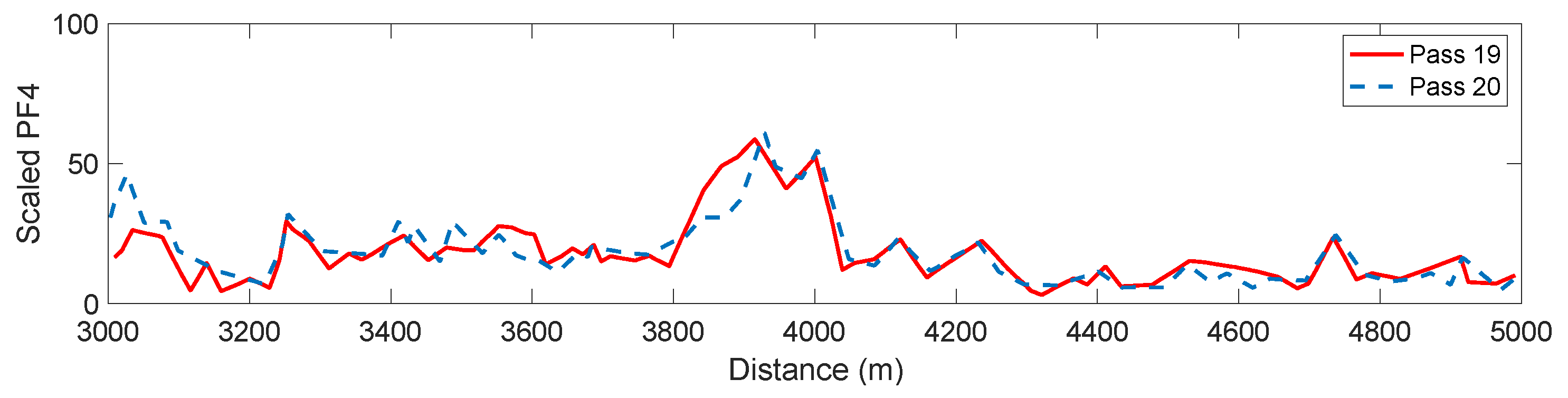
Even when data with speed less than 50 km/h are removed from the dataset, there is high influence of speed on signal energy. In some cases, this variability might cause fluctuations in calculated energy and it might de-emphasize the features caused by track faults. For example, the acceleration signals for two consecutive passes, Passes 19 and 20, are shown in Figure 8a for the zone, 3000 to 5000 m. Figure 8b shows the train forward speeds corresponding to these two passes. Figure 8c shows the PF5 of these two signals. The forward train speed of Pass 19 is about 30% less that Pass 20 in the range from 3000 to 3200 m, but it is increasing and catches up with the speed of Pass 20 at about 4000 m. There are two distance ranges in the signals where high energy levels are present; 3000 to 3100 m and 3800 to 4000 m. Figure 8c shows that there is a considerable difference in the energy of signals at the first range, while both of the signals give almost similar levels of energy for the second one. This shows that a higher forward speed creates a higher energy at the same section of track, with the lower speed of Pass 19 de-emphasizing the peak around 3000 to 3100 m.
The influence of forward speed on the signal amplitude is clearly not desirable for drive-by railway track monitoring.
A scaling method is proposed in order to minimize the effect of forward speed. Several scaling methods (linear, quadratic, etc.) were tested and showed a nonlinear relationship between the energy of vertical acceleration responses and the train forward speeds (horizontal speed). However, a linear scaling method is adopted, as it gives a reasonable performance while being simple and easy to apply. The linear scaling factor corrects the signal energy while using the corresponding train forward speed. To get consistent amplitudes for different passes at different speeds, a scaling factor using the train forward speed is applied:
where is the scaled amplitude at location , is an arbitrary average speed used as a baseline for all passes (taken to be 80 km/h here), is the speed of the train at location x, and is the amplitude obtained from the PD algorithm. Figure 9 shows the scaled PF4 for both passes 19 and 20 while using 80 km/h. Except for the first peak around 3020 m, the peaks are more consistent in the scaled PF4 for these passes.
There are several factors (e.g., change in the total mass of the train, temperature change, etc.) that impact the energy levels. However, the focus of this study is more on the impact of vehicle forward speed and the other data were not measured during the experiment.
5. Fault Detection on Dublin-Belfast Route
5.1. Fault Detection Method
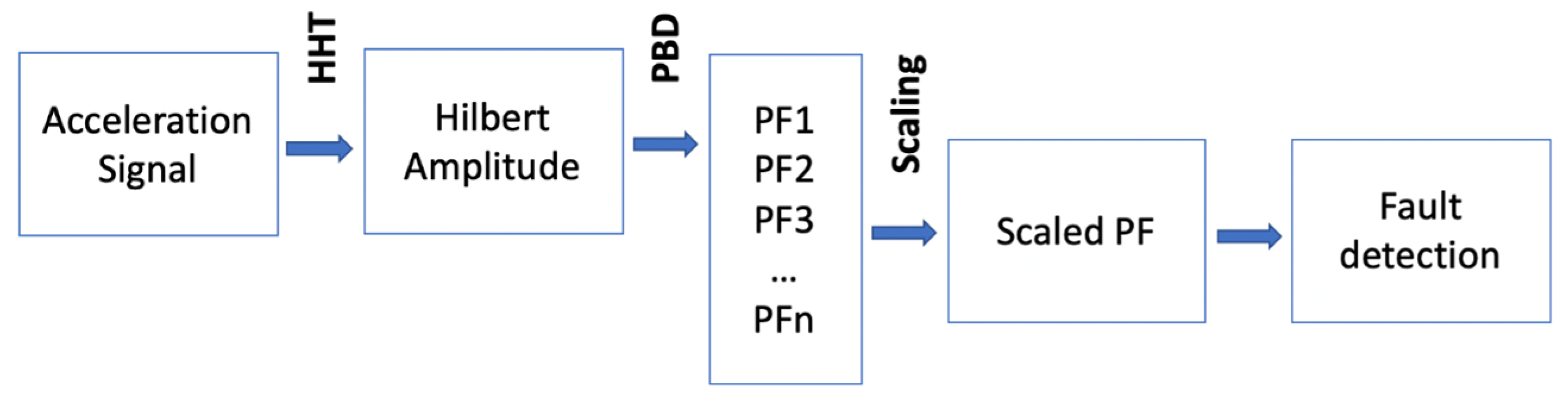
Figure 10 gives an overview of the proposed fault detection algorithm. The raw acceleration data are first processed using the Hilbert Huang Transform (HHT) method, as explained in Section 3.1, which results in Hilbert amplitudes. Subsequently, the Hilbert amplitudes are decomposed while using the PBD method explained in Section 3.2. The selected PF is then scaled using the scaling process that is explained in Section 4.2. Finally, the scaled PF is used to detect faults on the railway track. The procedure is employed in an experimental case study in the following sections.
5.2. Data Scaling
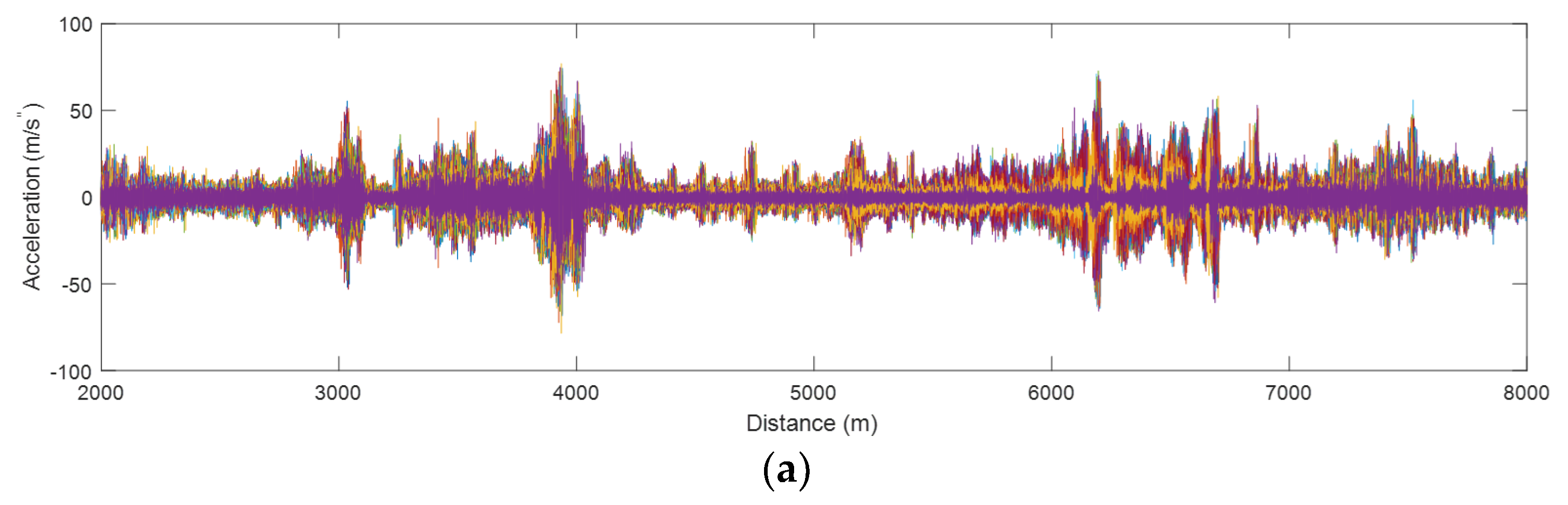
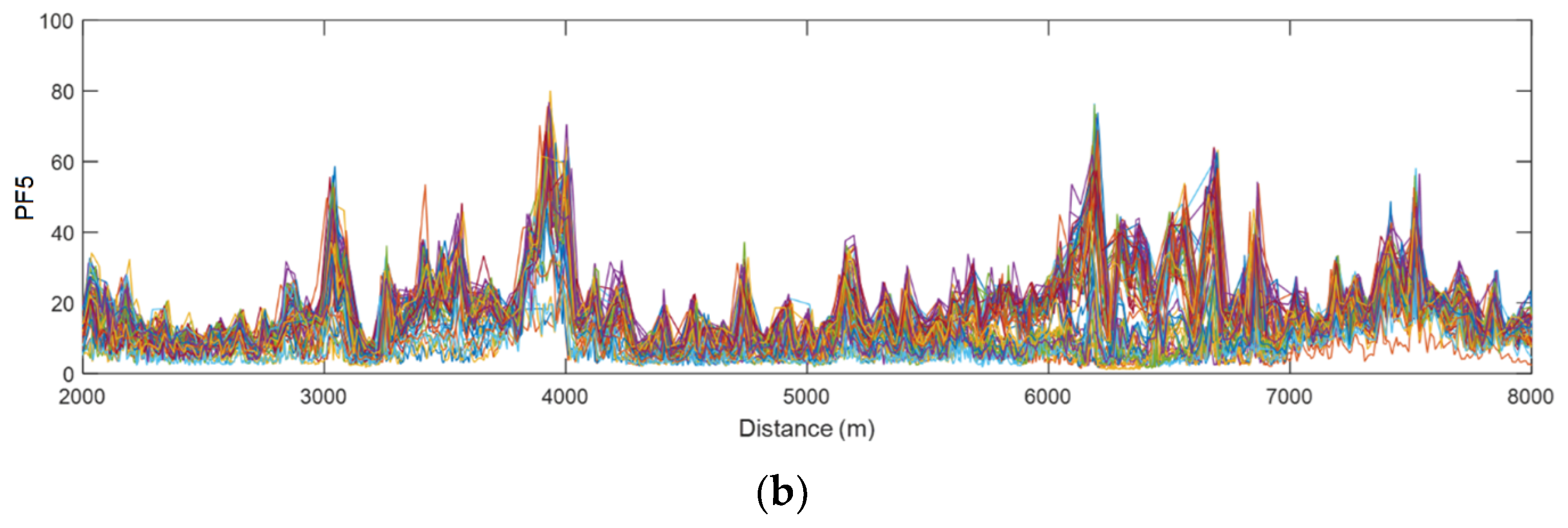
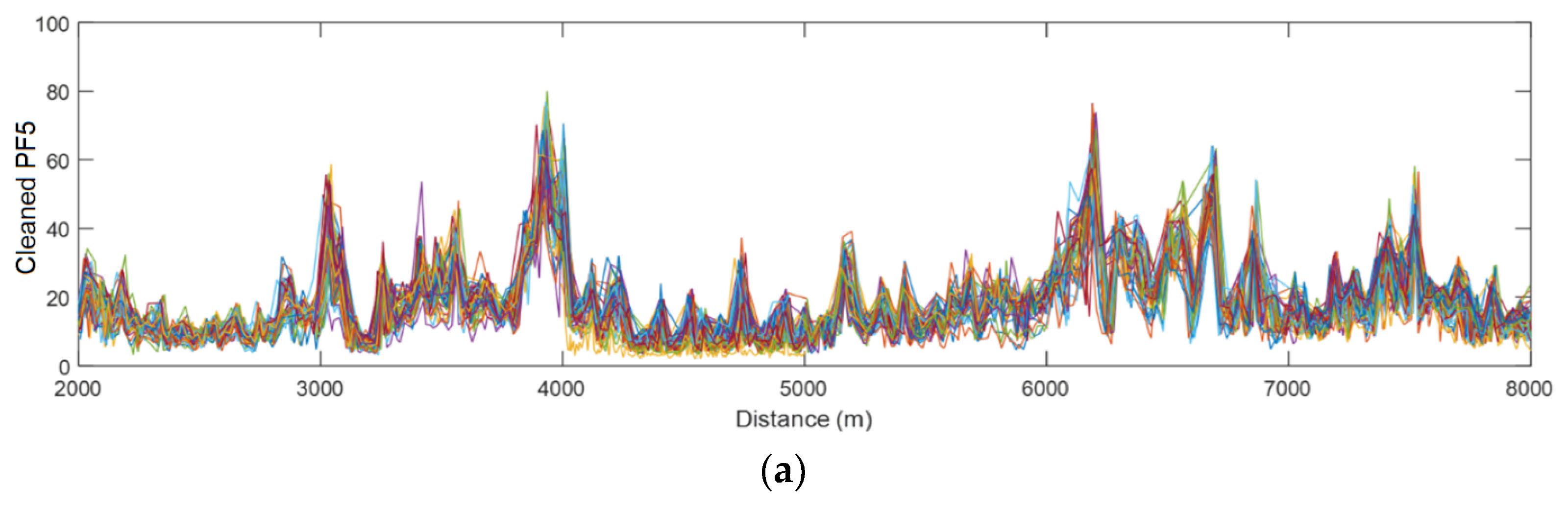
The TRV data shows several possible track defects in a zone between 2 to 8 km from Conolly station in Dublin. The measured bogie vertical accelerations from this 6 km of the Dublin-Belfast railway line is the dataset considered for fault detection. Figure 11a shows the 60 acceleration signals measured at the bogie. There are different energy levels in each signal, which makes it hard to infer the condition of the track. Figure 11b shows the PF5 of the Hilbert amplitudes of the signals that were calculated while using Equation (5). Although it constitutes an improvement, high variations remain between passes, e.g., between 6000 to 7000 m.
Figure 12 shows the forward speeds for all passes and show a great deal of variation. As proposed in Section 4.1, data are removed for any 1 km length in which the minimum forward speed of the train is less than 50 km/h. The 1 km segments for which data has been removed are shown in bold red in the figure. It can be seen that there are many passes between 5000 to 7000 m that need to be removed from the data set. This could explain the high amplitude variations in this zone in Figure 11b.
Figure 13a shows the cleaned version of Figure 11b, where segments of passes with speed below the limit have been removed. This figure clearly shows greater consistency in the amplitudes as compared to Figure 11b, particularly in the peaks. This is further improved with the energy scaling of Equation (5). The scaled amplitudes are plotted in Figure 13b and they can be seen to be more consistent than those of Figure 13a. Table 2 gives the average standrard deviations of the amplitudes in Figure 13a,b for different ranges. It shows that the average standard deviation of the data at all ranges has decreased after rescaling, which is a sign of greater consistency.
Figure 11 and Figure 13 show how the raw acceleration signals are processed to create a robust and reliable representation of the signal energy along the track. The mean value of the amplitudes in Figure 13b can be treated as a condition indictor for the track that can be used for long term monitoring. A current high energy level can be considered as a possible defect at the track. Therefore, monitoring the track condition while using the proposed indicator and keeping the energy level of the indicator minimum might be good practice for railway track maintenance.
5.3. Comparison of Results with Track Recording Vehicle Data
The locations in Figure 13 where the amplitudes exhibit high energy are inspected in this section for the purpose of fault detection. There are four main zones in Figure 13b that show high energy levels: around 3100 m, 3900 m, 6000–7000 m, and 7550 m. Irish Rail’s Track Recording Vehicle (TRV) monitored the track shortly after the acceleration measurements were taken. The TRV data are used here as a baseline to check the effectiveness of the proposed damage indicator.
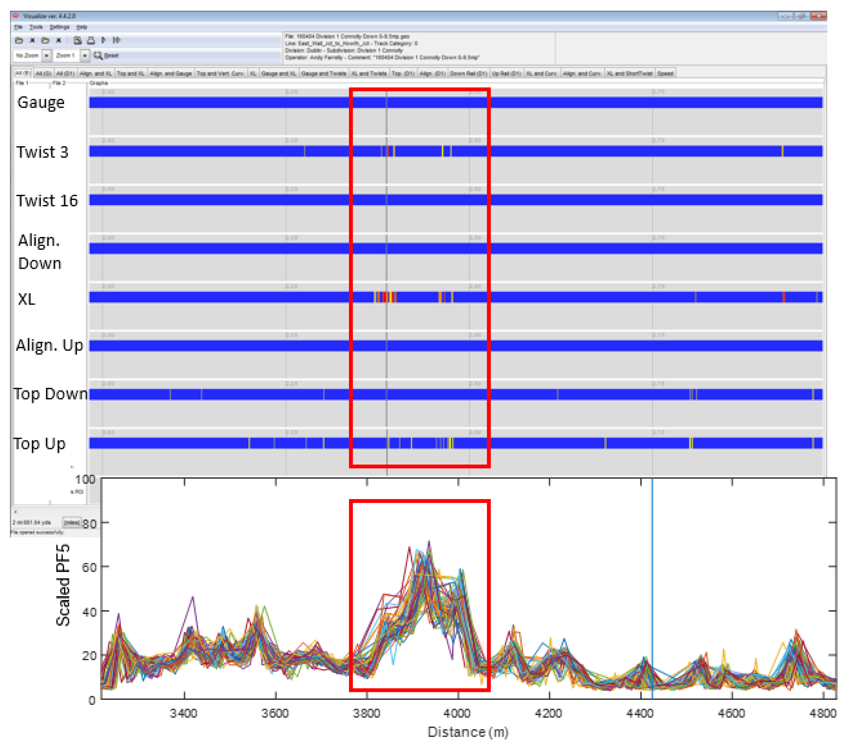
The scaled amplitudes around the second peak close to 3900 m are shown in Figure 14 with the corresponding TRV data. The TRV data includes eight track properties, named here using the colloquial terms and being represented by colour bars. The properties shown in this output (from the top) include ‘Gauge’ (track gauge), ‘Twist 3′ (3 m twist), ‘Twist 10′ (10 m twist), ‘Align Down’ (alignment (horizontal) of the down rail), ‘XL’ (cross level), ‘Align Up’ (alignment (horizontal) of the up rail), ‘Top Down’ (longitudinal level (vertical alignment) of the down rail), and ‘Top Up’ (longitudinal level (vertical alignment) of the up rail). These properties are defined in detail in EN 13848. The blue colour implies no irregularity or defect, while yellow, orange, and red indicate the alert and intervention limits that are defined by the standard.
The TRV data clearly show some defects between 3800 and 4000 m corresponding to the dominant peak in the scaled Hilbert amplitudes. The cross level parameter, ‘XL’, in the TRV data shows that the intervention limit has been exceeded at this location. Cross level is a measure of the difference in height of the running tables of both rails. It can be observed that this is caused by two changes in the longitudinal level of the up rail, which also manifests itself as a 3 m twist. This defect in the longitudinal level would have caused significant vertical motion of the bogie frame, which was measured by the sensor attached to the bogie. The resulting scaled amplitudes show a strong correlation between the Hilbert amplitude and recorded TRV damage.
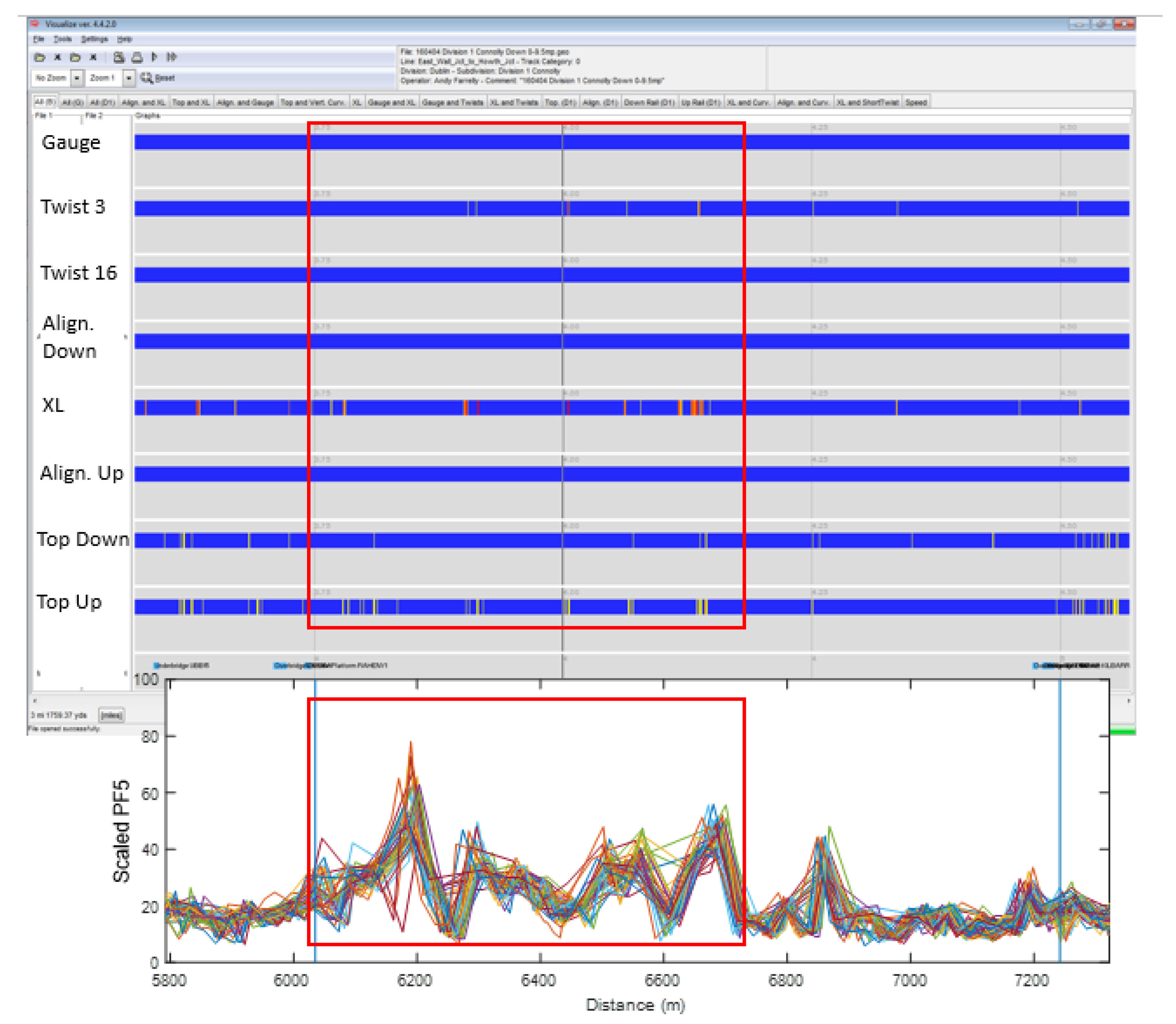
Figure 15 shows the scaled amplitudes and TRV data between 5800 to 7200 m, where there are also high energy levels. Again, the deviations in the vertical alignment of the up rail produce defects, which are also measured as defects in cross level and 3 m twist. The good match between the energy indicator and the TRV data confirms that the idea of drive-by train monitoring has good potential for railway track monitoring while using an in-service vehicle.
Figure 14 and Figure 15 are two samples that show the effectiveness of the proposed method. However, further work is needed to improve the accuracy of the locations and also find the types of the faults detected by this method. For example, the accuracy of the defect locations is a function of the performance of the GNSS under different train forward speeds. This could create some levels of mismatching between different passes. There is also some error in the PBD process in terms of the accuracy of the peak locations. However, there is reasonable consistency over several passes, which indicates acceptable performance.
6. Conclusions
In this paper, the idea of drive-by railway track monitoring is investigated while using field measurements. An operational train from the Irish Rail fleet is instrumented using accelerometers installed on the train bogie. The train location and forward velocity are recorded while using a GPS system. A data set including acceleration and train velocity measurements from 60 passes on the Dublin-Belfast line is studied. The energy of the signals is extracted from the amplitudes of the accelerations using a Hilbert transform and considered as a track condition indicator. It is shown that, when the train has a forward speed less than 50 km/h, the energy indicator is no longer reliable. The data set is cleaned by removing these low speed passes for each 1 km data segment and the remaining passes are scaled using the train forward speed. It is demonstrated that the scaled amplitudes provide good repeatability for multiple measurements and they show considerable potential for drive-by track monitoring. The scaled amplitudes for a 6 km dataset are compared with TRV measurements. This confirms that the locations with high energy levels correspond to parts of the track that exhibit faults in the TRV data.
Author Contributions
Conceptualization, A.M. and P.Q.; methodology, A.M.; formal analysis and investigation, A.M and P.Q.; writing—original draft preparation, A.M. and E.OB.; writing—review and editing, A.M., E.OB. and P.Q.; supervision, E.OB. and C.B.
Funding
The project has received funding from the European Union’s Seventh Framework Programme for research, technological development and demonstration under grant agreement number 607524. The authors are thankful for this support. The authors wish to acknowledge the financial support received from Science Foundation Ireland under the US-Ireland Research Partnership Scheme. This research also was funded by the ‘Irish Research Council New Foundations’.
Conflicts of Interest
The authors declare no conflict of interest.
References
- Malekjafarian, A.; Brien, E.J.O.; Golpayegani, F. Indirect Monitoring of Critical Transport Infrastructure: Data Analysis and Signal Processing. In Data Anlytics Applications for Smart Cities; Alavi, A.H., Buttlar, W.G., Eds.; Auerbach/CRC Press: Boston, MA, USA, 2018. [Google Scholar]
- Berggren, E.G.; Nissen, A.; Paulsson, B.S. Track deflection and stiffness measurements from a track recording car. Proc. Inst. Mech. Eng. Part F J. Rail Rapid Transit. 2014, 228, 570–580. [Google Scholar] [CrossRef]
- Malekjafarian, A.; McGetrick, P.J.; Brien, E.J.O. A Review of Indirect Bridge Monitoring Using Passing Vehicles. Shock Vib. 2015, 2015, 286139. [Google Scholar] [CrossRef]
- Malekjafarian, A.; OBrien, E.J. On the use of a passing vehicle for the estimation of bridge mode shapes. J. Sound Vib. 2017. [Google Scholar] [CrossRef]
- Flintsch, G.W.; Ferne, B.; Diefenderfer, B.; Katicha, S.; Bryce, J.; Nell, S. Evaluation of Traffic-Speed Deflectometers. Transp. Res. Rec. 2012, 37–46. [Google Scholar] [CrossRef]
- Heirich, O.; Lehner, A.; Robertson, P.; Strang, T. Measurement and analysis of train motion and railway track characteristics with inertial sensors. In Proceedings of the 2011 14th International IEEE Conference on Intelligent Transportation Systems (ITSC), Washington, DC, USA, 5–7 October 2011. [Google Scholar]
- Weston, P.; Roberts, C.; Yeo, G.; Stewart, E. Perspectives on railway track geometry condition monitoring from in-service railway vehicles. Veh. Syst. Dyn. 2015, 53, 1063–1091. [Google Scholar] [CrossRef]
- Fallah Nafari, S.; Gül, M.; Roghani, A.; Hendry, M.T.; Cheng, J.R. Evaluating the potential of a rolling deflection measurement system to estimate track modulus. Proc. Inst. Mech. Eng. Part F-J. Rail Rapid Transit. 2018, 232, 14–24. [Google Scholar] [CrossRef]
- Bar-Am, M. On-Train Rail Track Monitoring System. Google Patents. U.S. 8,942,426, 27 January 2015. [Google Scholar]
- Fosburgh, B.A.; Nichols, M.E.; Holmgren, P.M.; Larsson, N.T. Railway Track Monitoring. Google Patents. U.S. 9,810,533, 7 November 2017. [Google Scholar]
- OBrien, E.J.; Quirke, P.; Bowe, C.; Cantero, D. Determination of railway track longitudinal profile using measured inertial response of an in-service railway vehicle. Struct. Health Monit. 2017, 17, 1425–1440. [Google Scholar] [CrossRef]
- Zemp, A.; Muller, R.; Hafner, M. Characterization of Train-Track Interactions based on Axle Box Acceleration Measurements for Normal Track and Turnout Passages. In Proceedings of the Eurodyn 2014: Ix International Conference on Structural Dynamics, Porto, Portugal, 30 June–2 July 2014; pp. 827–833. [Google Scholar]
- Wei, Z.; Núñez, A.; Li, Z.; Dollevoet, R. Evaluating Degradation at Railway Crossings Using Axle Box Acceleration Measurements. Sensors 2017, 17, 2236. [Google Scholar]
- Oregui, M.; Li, S.; Núñez, A.; Li, Z.; Carroll, R.; Dollevoet, R. Monitoring bolt tightness of rail joints using axle box acceleration measurements. Struct. Control Health Monit. 2017, 24, e1848. [Google Scholar] [CrossRef]
- Molodova, M.; Oregui, M.; Núñez, A.; Li, Z.; Dollevoet, R. Health condition monitoring of insulated joints based on axle box acceleration measurements. Eng. Struct. 2016, 123, 225–235. [Google Scholar] [CrossRef]
- Salvador, P.; Naranjo, V.; Insa, R.; Teixeira, P. Axlebox accelerations: Their acquisition and time-frequency characterisation for railway track monitoring purposes. Measurement 2016, 82, 301–312. [Google Scholar] [CrossRef]
- Real, J.; Salvador, P.; Montalbán, L.; Bueno, M. Determination of rail vertical profile through inertial methods. Proc. Inst. Mech. Eng. Part F J. Rail Rapid Transit. 2011, 225, 14–23. [Google Scholar] [CrossRef]
- Quirke, P.; Cantero, D.; OBrien, E.J.; Bowe, C. Drive-by detection of railway track stiffness variation using in-service vehicles. Proc. Inst. Mech. Eng. Part F J. Rail Rapid Transit. 2017, 231, 498–514. [Google Scholar] [CrossRef]
- Le Pen, L.; Watson, G.; Powrie, W.; Yeo, G.; Weston, P.; Roberts, C. The behaviour of railway level crossings: Insights through field monitoring. Transp. Geotech. 2014, 1, 201–213. [Google Scholar] [CrossRef]
- Cantero, D.; Basu, B. Railway infrastructure damage detection using wavelet transformed acceleration response of traversing vehicle. Struct. Control Health Monit. 2015, 22, 62–70. [Google Scholar] [CrossRef]
- Chen, S.; Cerda, F.; Rizzo, P.; Bielak, J.; Garrett, J.H.; Kovačević, J. Semi-Supervised Multiresolution Classification Using Adaptive Graph Filtering With Application to Indirect Bridge Structural Health Monitoring. IEEE Trans. Signal Process. 2014, 62, 2879–2893. [Google Scholar] [CrossRef]
- Tsai, H.C.; Wang, C.Y.; Huang, N.E.; Kuo, T.W.; Chieng, W.H. Railway track inspection based on the vibration response to a scheduled train and the Hilbert-Huang transform. Proc. Inst. Mech. Eng. Part F-J. Rail Rapid Transit. 2015, 229, 815–829. [Google Scholar] [CrossRef]
- Lederman, G.; Chen, S.; Garrett, J.; Kovačević, J.; Noh, H.Y.; Bielak, J. Track-monitoring from the dynamic response of an operational train. Mech. Syst. Signal Process. 2017, 87, 1–16. [Google Scholar] [CrossRef]
- Tsunashima, H.; Naganuma, Y.; Matsumoto, A.; Mizuma, T.; Mori, H. Condition monitoring of railway track using in-service vehicle. Reliab. Saf. Railw. 2012, 12, 334–356. [Google Scholar]
- Kobayashi, T.; Naganuma, Y.; Tsunashima, H. Condition Monitoring of Shinkansen Tracks based on Inverse Analysis. Int. J. Perform. Eng. 2014, 10, 703–708. [Google Scholar]
- Paixão, A.; Fortunato, E.; Calçada, R. Smartphone’s Sensing Capabilities for On-Board Railway Track Monitoring: Structural Performance and Geometrical Degradation Assessment. Adv. Civ. Eng. 2019, 2019, 1729153. [Google Scholar] [CrossRef]
- Lederman, G.; Chen, S.; Garrett, J.H.; Kovačević, J.; Noh, H.Y.; Bielak, J. Track monitoring from the dynamic response of a passing train: A sparse approach. Mech. Syst. Signal Process. 2017, 90, 141–153. [Google Scholar] [CrossRef]
- Liu, K.; Reynders, E.; De Roeck, G.; Lombaert, G. Experimental and numerical analysis of a composite bridge for high-speed trains. J. Sound Vib. 2009, 320, 201–220. [Google Scholar] [CrossRef]
- Kouroussis, G.; Verlinden, O.; Conti, C. Free field vibrations caused by high-speed lines: Measurement and time domain simulation. Soil Dyn. Earthq. Eng. 2011, 31, 692–707. [Google Scholar] [CrossRef]
- Domenech, A.; Museros, P.; Martinez-Rodrigo, M.D. Influence of the vehicle model on the prediction of the maximum bending response of simply-supported bridges under high-speed railway traffic. Eng. Struct. 2014, 72, 123–139. [Google Scholar] [CrossRef]
- Antolín, P.; Zhang, N.; Goicolea, J.M.; Xia, H.; Astiz, M.Á.; Oliva, J. Consideration of nonlinear wheel-rail contact forces for dynamic vehicle-bridge interaction in high-speed railways. J. Sound Vib. 2013, 332, 1231–1251. [Google Scholar] [CrossRef]
- Quirke, P. Drive-by detection of railway track longitudinal profile, stiffness and bridge damage. In School of Civil Engineering; University College Dublin: Dubli, Ireland, 2017. [Google Scholar]
- Huang, N.E.; Shen, Z.; Long, S.R.; Wu, M.C.; Shih, H.H.; Zheng, Q.; Yen, N.C.; Tung, C.C.; Liu, H.H. The empirical mode decomposition and the Hilbert spectrum for nonlinear and non-stationary time series analysis. Proc. R. Soc. A-Math. Phys. Eng. Sci. 1998, 454, 903–995. [Google Scholar] [CrossRef]
Figure 1.
The measurement set up: (a) the instrumented train, and (b) the triaxial accelerometer.

Figure 2.
The acceleration signals of the first five passes.

Figure 3.
Frequency content of the accelerations of Pass 3, (a) the Fast Fourier Transform (FFT) spectrum and (b) Short Time FFT (STFFT) spectrum.
Figure 3.
Frequency content of the accelerations of Pass 3, (a) the Fast Fourier Transform (FFT) spectrum and (b) Short Time FFT (STFFT) spectrum.

Figure 4.
Hilbert amplitude of a sample acceleration signal, (a) 6500 to 6600 m, and (b) 6500 to 6510 m.
Figure 4.
Hilbert amplitude of a sample acceleration signal, (a) 6500 to 6600 m, and (b) 6500 to 6510 m.

Figure 5.
The peak decomposition (PD) process.

Figure 6.
Comparison of the raw acceleration, Peak 4, Peak 5, and average energy.

Figure 7.
Forward speed of the first five passes.

Figure 8.
Two sample signals, (a) the accelerations, (b) the forward speed, and (c) the energy level (PF 4).
Figure 8.
Two sample signals, (a) the accelerations, (b) the forward speed, and (c) the energy level (PF 4).

Figure 9.
The scaled energy level for two sample signals (PF 4).

Figure 10.
The fault detection algorithm.

Figure 11.
Sixty passes of data: (a) Acceleration signals, and (b) PF5 of Hilbert amplitudes.


Figure 12.
The train forward speeds for all 60 passes (red indicates 1 km segments for which data has been removed).
Figure 12.
The train forward speeds for all 60 passes (red indicates 1 km segments for which data has been removed).

Figure 13.
The PF5 (a) after cleaning to remove segments below the speed limit, (b) after rescaling the cleaned signals.
Figure 13.
The PF5 (a) after cleaning to remove segments below the speed limit, (b) after rescaling the cleaned signals.


Figure 14.
The Track Recording Vehicle (TRV) data and scaled amplitudes.

Figure 15.
The TRV data and scaled amplitudes.


Table 1.
The main track parameters for drive-by monitoring using inertial measurements.
| Category number | Monitoring Purpose | Example | Literature |
|---|---|---|---|
| 1 | Track components | Crossings, joints, turnout frogs, squats etc. | [12,13,14,15,16] |
| 2 | Track profile | Stiffness profile, elevation profile | [11,17,18,19] |
| 3 | Others | Track replacement, tamping, rail bump and rail surface irregularities | [20,21,22,23] |
Table 2.
Statistical properties of the signals before and after rescaling.
| Average Standard Deviation | ||||||
|---|---|---|---|---|---|---|
| Range | 2000–3000 m | 3000–4000 m | 4000–5000 m | 5000–6000 m | 6000–7000 m | 7000–8000 m |
| Not-scaled | 3.42 | 6.68 | 4.43 | 4.20 | 8.15 | 4.82 |
| Scaled | 2.96 | 5.80 | 3.49 | 2.92 | 6.61 | 3.95 |
© 2019 by the authors. Licensee MDPI, Basel, Switzerland. This article is an open access article distributed under the terms and conditions of the Creative Commons Attribution (CC BY) license (http://creativecommons.org/licenses/by/4.0/).
Share and Cite
MDPI and ACS Style
Malekjafarian, A.; OBrien, E.; Quirke, P.; Bowe, C. Railway Track Monitoring Using Train Measurements: An Experimental Case Study. Appl. Sci. 2019, 9, 4859. https://0-doi-org.brum.beds.ac.uk/10.3390/app9224859
AMA Style
Malekjafarian A, OBrien E, Quirke P, Bowe C. Railway Track Monitoring Using Train Measurements: An Experimental Case Study. Applied Sciences. 2019; 9(22):4859. https://0-doi-org.brum.beds.ac.uk/10.3390/app9224859
Chicago/Turabian StyleMalekjafarian, Abdollah, Eugene OBrien, Paraic Quirke, and Cathal Bowe. 2019. "Railway Track Monitoring Using Train Measurements: An Experimental Case Study" Applied Sciences 9, no. 22: 4859. https://0-doi-org.brum.beds.ac.uk/10.3390/app9224859
Note that from the first issue of 2016, this journal uses article numbers instead of page numbers. See further details here.