Three Rapid Methods for Averaging GPS Segments


School of Computing, University of Eastern Finland, 80101 Joensuu, Finland
*
Author to whom correspondence should be addressed.
Appl. Sci. 2019, 9(22), 4899; https://0-doi-org.brum.beds.ac.uk/10.3390/app9224899
Submission received: 8 October 2019
/
Revised: 25 October 2019
/
Accepted: 12 November 2019
/
Published: 15 November 2019
(This article belongs to the Section Electrical, Electronics and Communications Engineering)
Abstract
:Extracting road segments by averaging GPS trajectories is very challenging. Most existing averaging strategies suffer from high complexity, poor accuracy, or both. For example, finding the optimal mean for a set of sequences is known to be NP-hard, whereas using Medoid compromises the quality. In this paper, we introduce three extremely fast and practical methods to extract the road segment by averaging GPS trajectories. The methods first analyze three descriptors and then use either a simple linear model or a more complex curvy model depending on an angle criterion. The results provide equal or better accuracy than the best existing methods while being very fast, and are therefore suitable for real-time processing. The proposed method takes only 0.7% of the computing time of the best-tested baseline method, and the accuracy is also slightly better (62.2% vs. 61.7%).
1. Introduction
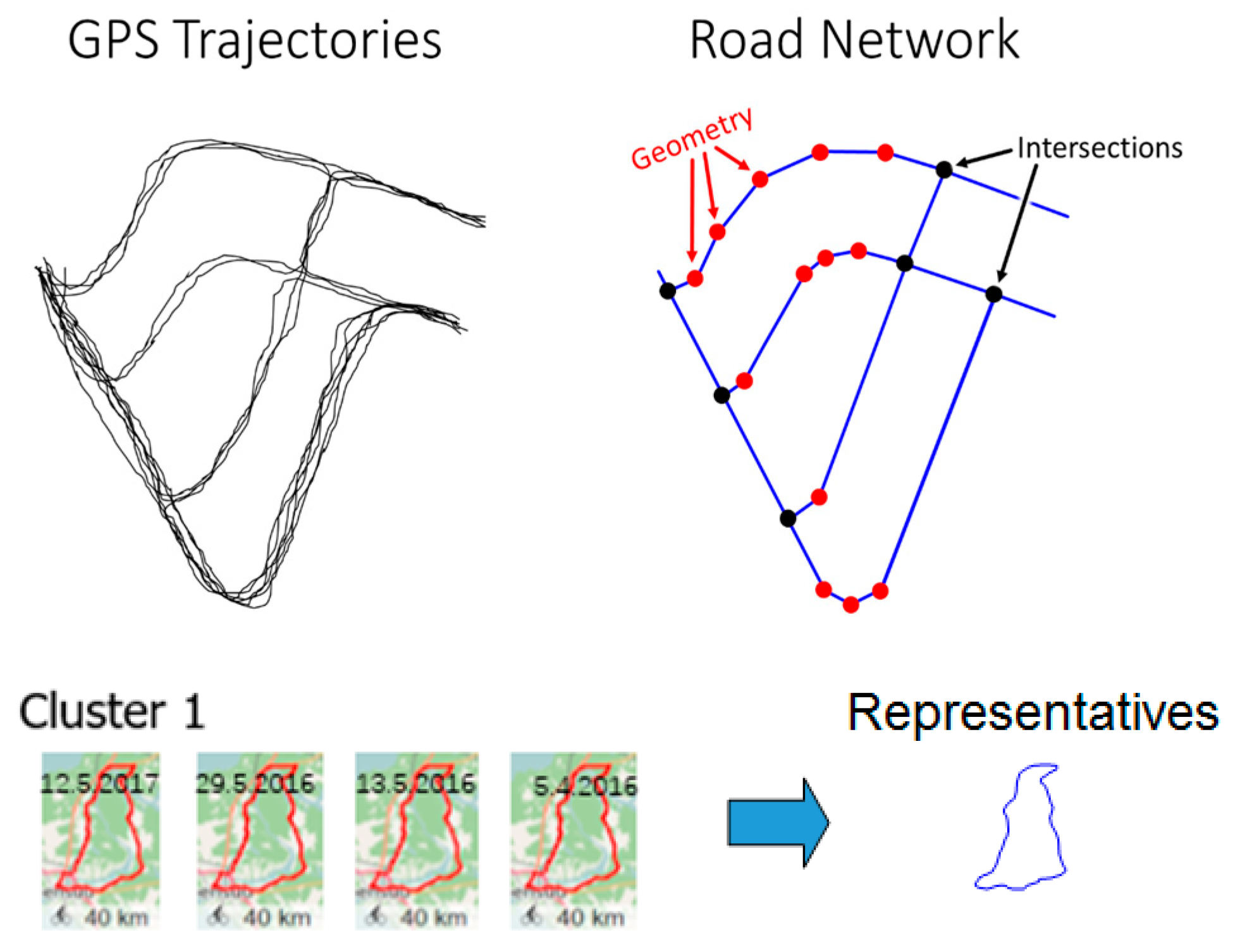
We study the problem of finding a good representative of a set of GPS trajectories. Solutions are needed in several applications such as extracting road network, trajectory clustering, and calculating average routes for taxi trips, see Figure 1. The input is an ordered sequence of geographical points (latitude, longitude), and the output is a polygon that approximates the path traveled.
The problem is closely related to averaging time series, which has been studied actively in recent years in the context of dynamic time warping (DTW) distance. The common problem is that the observations may have been collected with different frequency, and the number of samples varies across the sequences. The major issue is how to align the sequences before averaging. Earlier studies have considered the problem as multiple sequence alignment (MSA), which is equivalent to the Steiner sequence [1]. However, it was recently shown that the multiple alignment approach does not guarantee optimality [2].
It is possible to solve the averaging problem by using “Mean”, which is defined as any sequence that minimizes the sum of squared distances to all the input sequences:
where X = {x1, x2, …, xk} is the set of input sequences and C is the mean. This definition defines averaging as an optimization problem. However, the search space is huge, and exhaustive search by enumeration is not feasible. An exponential time algorithm for solving the exact DTW-mean was recently given in [2], but the problem was shown to be NP-hard concerning the number of sequences [3].
The GPS trajectories differ from time series in a few ways. First, the alignment of the time series is performed in the time domain, whereas the GPS points need to be aligned in geographical space. Second, GPS data can be noisy. This means that the mean might not even be the best solution to the problem.
The averaging problem of GPS trajectories has been recently studied in a Segment averaging challenge (http://cs.uef.fi/sipu/segments/), with several new solutions proposed [4]. Most methods in the competition apply the four-step procedure shown in Figure 2. Some trajectories can be stored in reverse order, and reordering of the sequences is needed. Outlier removal is commonly applied to reduce the effect of the noisy trajectories. After these steps, the problem reduces to normal sequence averaging. Postprocessing by polygonal approximation is sometimes also done to simplify the final representation.
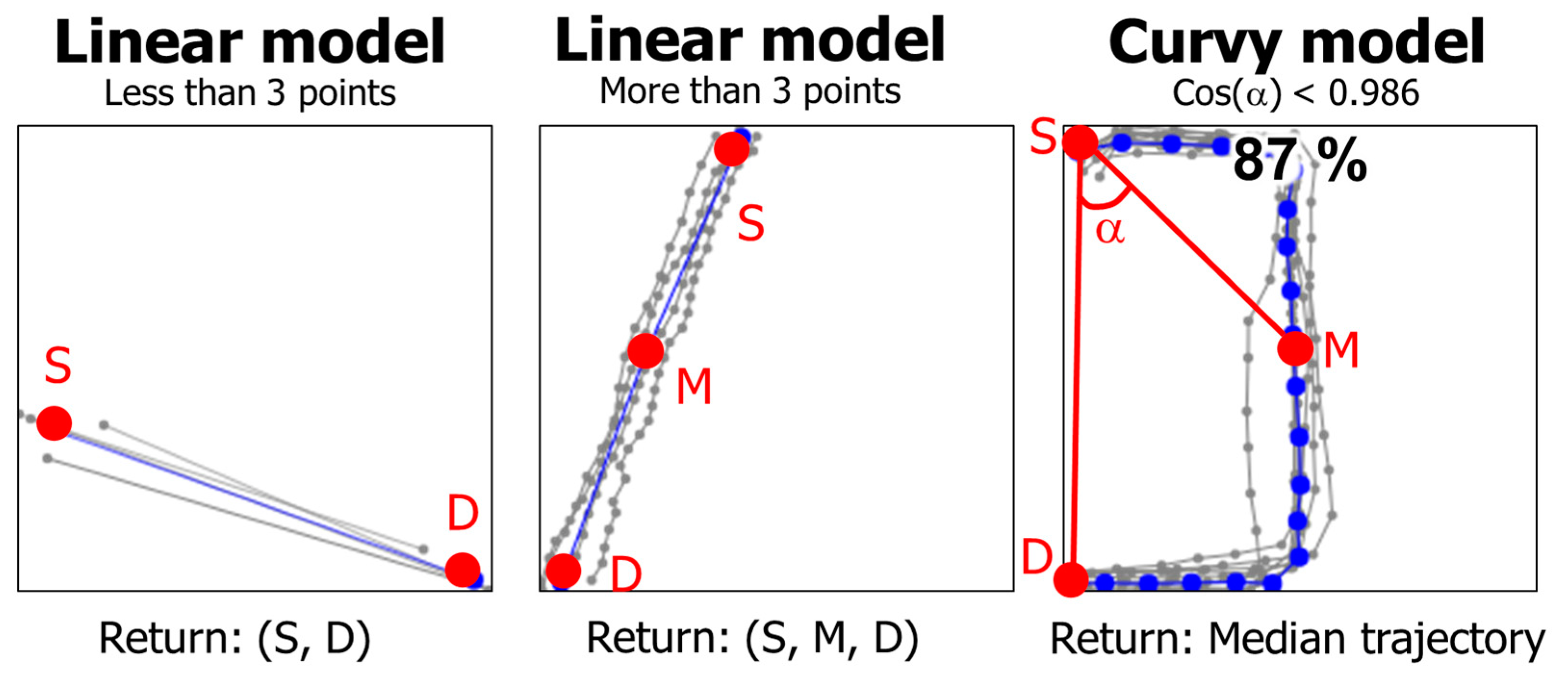
Although several reasonable solutions have been proposed, several of them are rather complicated, and some also suffer from high time complexity. In this paper, we present three rapid and simple methods based on analyzing three descriptors of the curves: start (S), middle (M), and destination (D), see Figure 3. If the trajectory resembles a line, a simple linear model with 3 points is produced; except when no intermediate points exist. Otherwise, a more complex curvy model is applied as a backup. Three methods are considered for this: Median, Medoid, and Divide-and-Conquer.
2. Existing Works on Segment Averaging
In [5], average segments (called “centerline”) were used for k-means clustering of the GPS trajectories to detect road lanes. The averaging method was later defined in [6] based on piecewise linear regression. The data is treated as an unordered set of points for which piecewise polynomials are fit with continuity conditions at the knot points [7]. The drawback of using regression is that we lose the information in which order points were collected, which makes the problem harder to solve. In the Segment averaging challenge [4], only one proposal was based on the regression approach, and its performance was not among the best.
Recent solutions consider the problem as sequence averaging and apply methods from a time series context using dynamic time warping as the distance function. For example, the CellNet segment averaging [8] takes the shortest path as the initial guess [9] and then applies the Majorize-minimize iterative algorithm [1] to estimate the mean. Another iterative algorithm uses kernelized time elastic averaging (iTEKA) for the averaging [10]. It considers all possible alignment paths and integrates a forward and backward alignment principle jointly.
Medoid is an alternative approach to mean. It is also defined as an optimization problem but with the difference that, instead of allowing any sequence, Medoid is selected as one of the input sequences. The problem can then be solved brute force by calculating all pairwise distances and selecting the sequence that minimizes the optimization function. Possible functions to measure the distance (or similarity) between GPS trajectories have been extensively studied in [11] and tested with the Medoid in [4]. In this paper, we use Hausdorff distance [12], as it is invariant to the travel order of the trajectories, and it provides competitive results among the other choices.
Medoid has two main drawbacks: First, it requires O(k2) distance calculations, where k is the number of trajectories. Standard implementations of distance functions like dynamic time warping usually require O(n2), where n is the number of points in the longest trajectory. Thus, the total time complexity can be as high as O(k2n2). Another drawback is that Medoid is limited to be one of the input trajectories, which can be a poor approximation of the average segment, especially if k is small.
3. Three Rapid Methods
The expected input for the algorithm is a set of trajectories; each consisting of an ordered sequence of locations (x, y). We assume that the trajectories provide point-to-point paths roughly from the same target and to the same destination locations. The direction of the travelling is not defined, i.e., some of the trajectories may have reverse direction; GPS errors are expected.
We next present three new methods for solving the problem:
- RapSeg-A: Median for curvy segments
- RapSeg-B: Medoid for curvy segments
- RapSeg-C: Divide-and-conquer approach
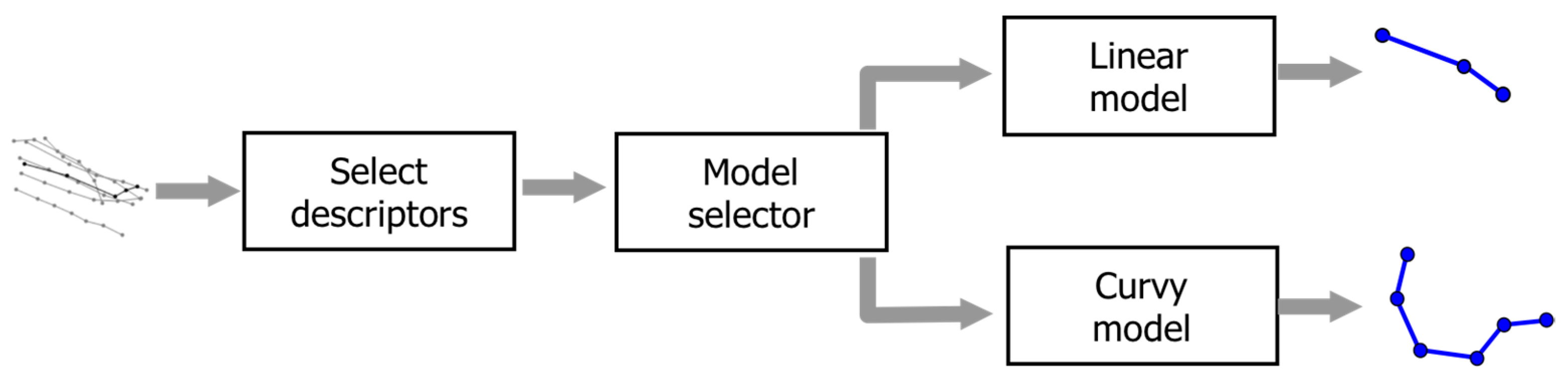
All methods use the same overall structure, as shown in Figure 4. Three descriptors are first calculated to describe the set of trajectories. Based on these descriptors, we estimate whether a simple linear model can describe the set, or a more complex model is necessary. We design two alternative models for these: the linear model and the curvy model.
3.1. Descriptors and Model Selector
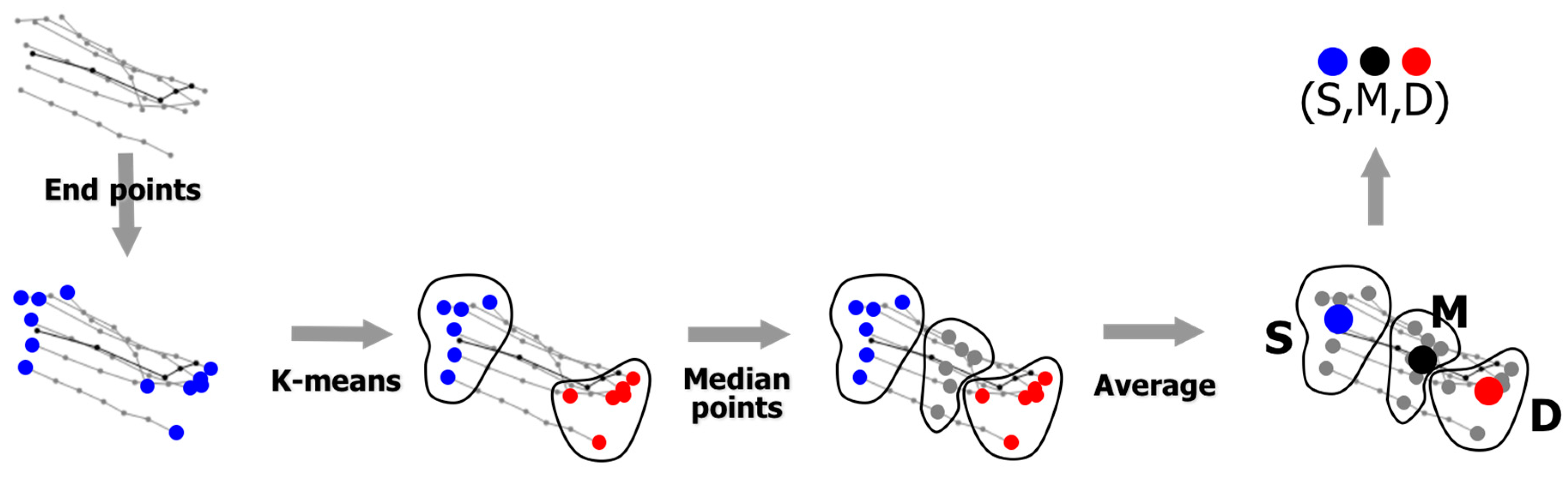
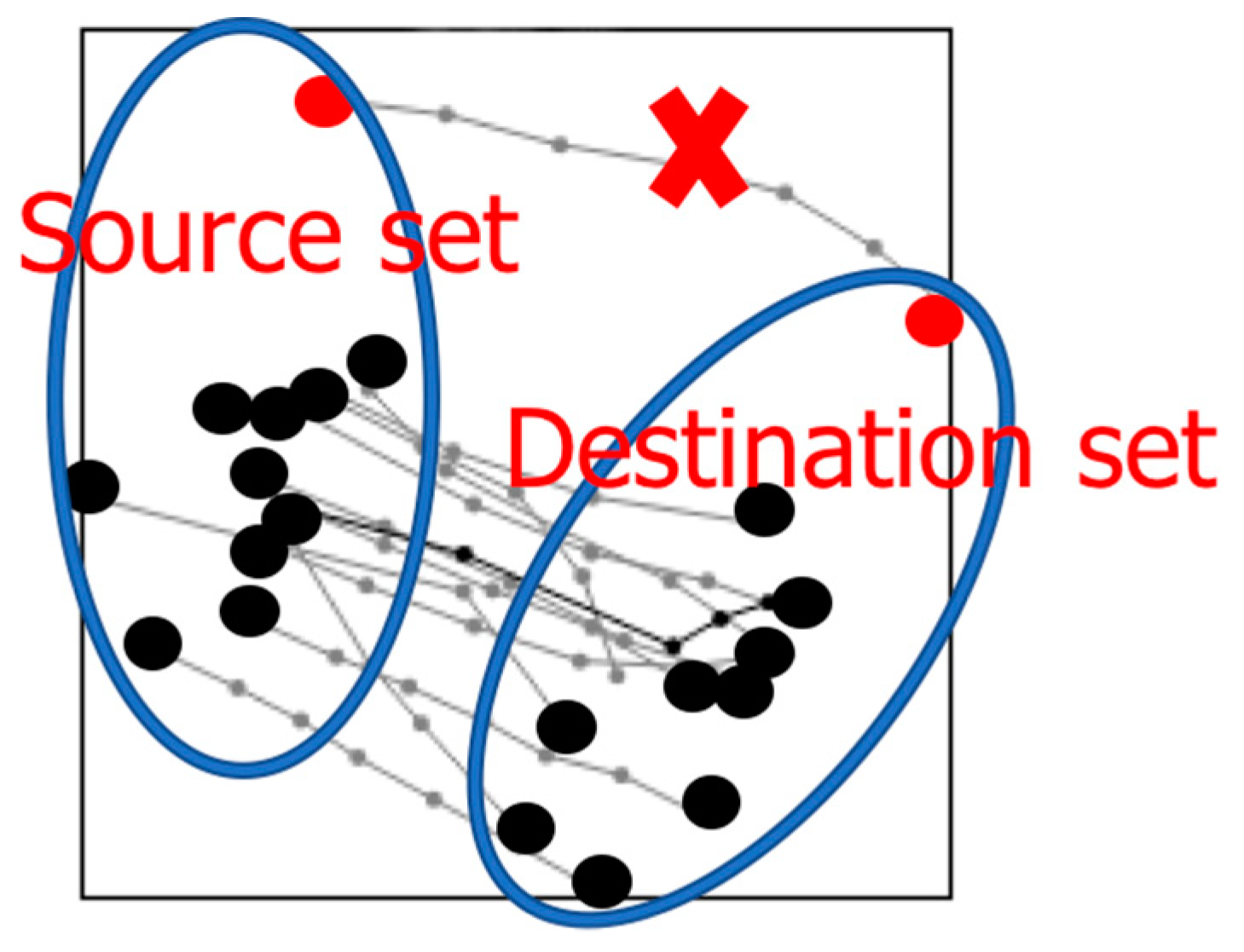
We calculate three descriptors to estimate the segment: source (S), median (M), and destination (D). We first select the endpoints from all trajectories and cluster them by k-means into two clusters. We denote these two clusters as source set and destination set for simplicity. As the method is invariant to the travel direction, the order of S and D can be chosen arbitrarily. Next, we analyze the trajectories and select the median (middle point) from every trajectory to get median set. Finally, we calculate the average (centroid) of each of those three sets to produce the triple (S, M, D). The process is summarized in Figure 5.
The descriptors are then used to decide whether the set can be described by a linear model. We compare the straight line SD against the two-segment line SMD, which makes detour via the median point M. The more the detour deviates from the direct connection, the less likely a simple linear model is suitable to describe the segment. The exact criterion is the angle ∠SDM and ∠DSM. If the cosine of the angle is less than a threshold value, we use a curvy model. We call the method as Rapid Segment (RapSeg), see Algorithm 1 and Figure 3.
| Algorithm 1: RapSeg (X, T): |
| 1: Input: GPS trajectories: X; threshold value: T 2: Output: representative: Y 3: S, M, D ← LineSegment(X); 4: IF cos(∠SDM) ≤ T || cos(∠DSM) ≤ T: 5: Y = CurveSegment(X); 6: ELSE: 7: Y = [S, M, D]; |
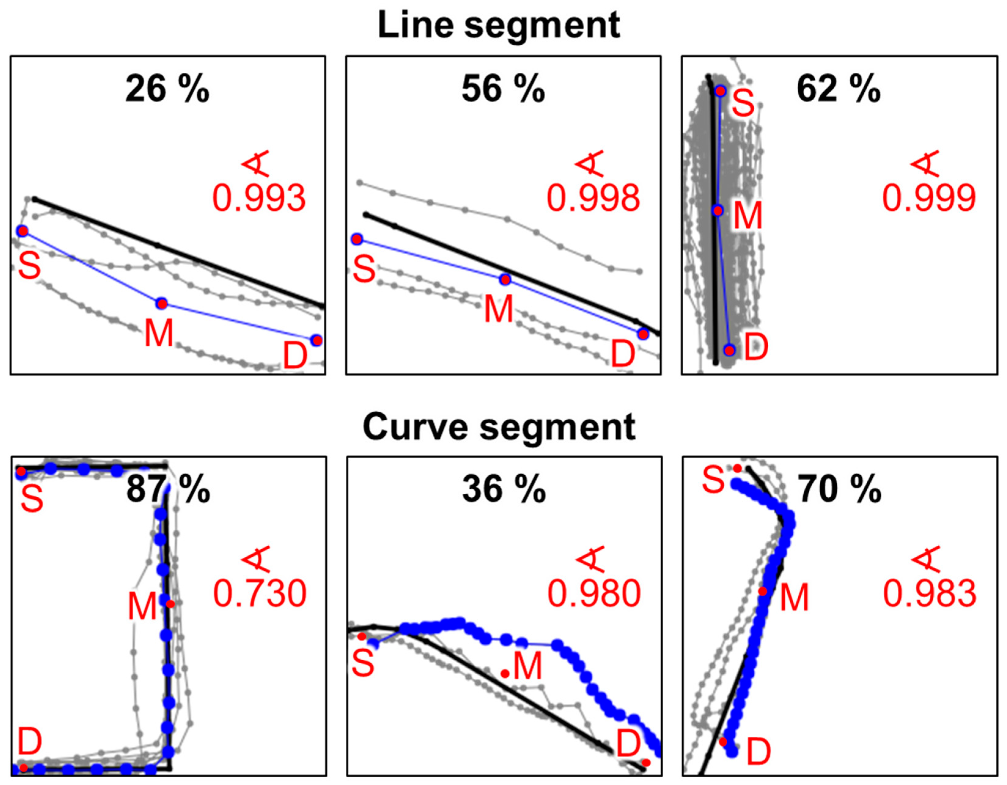
Examples of sets and their descriptors are shown in Figure 6. The first four examples have an only slight change of direction, and the linear model is therefore applied. The four examples below did not meet the angle criterion, and the curvy model is applied. Examples are shown using the median segment.
3.2. Linear Model
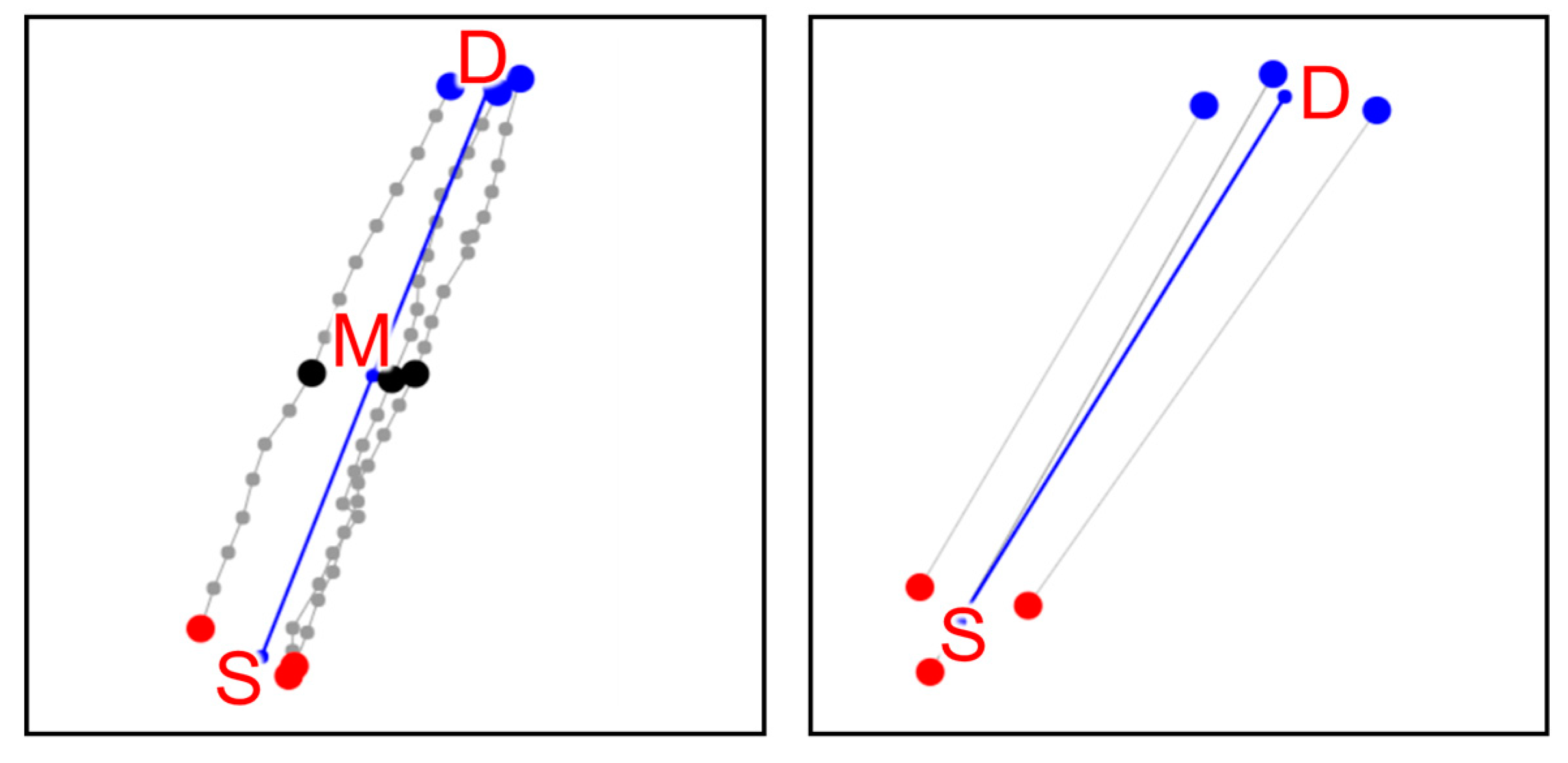
Our linear model is straightforward. We use the triple (S, M, D) as a three-point model to represent the segment. Algorithm 2 details the process, and examples are shown in Figure 7. Only in the case when all trajectories have only two points, the set M becomes empty, and we output only the pair (S, D) as the model.
| Algorithm 2: LineSegment (X): |
| 1: Input: GPS trajectories: X 2: Output: representative: Y 3: EndPoints ← Take the first and last point of every trajectory in X; 4: S, D ← K-meansClustering(EndPoints, K = 2); 5: MidPoints ← Take median point of every trajectory in X; 6: M ← Average(MidPoints); 7: Y = [S, M, D]; |
3.3. Curvy Model A: MEDIAN
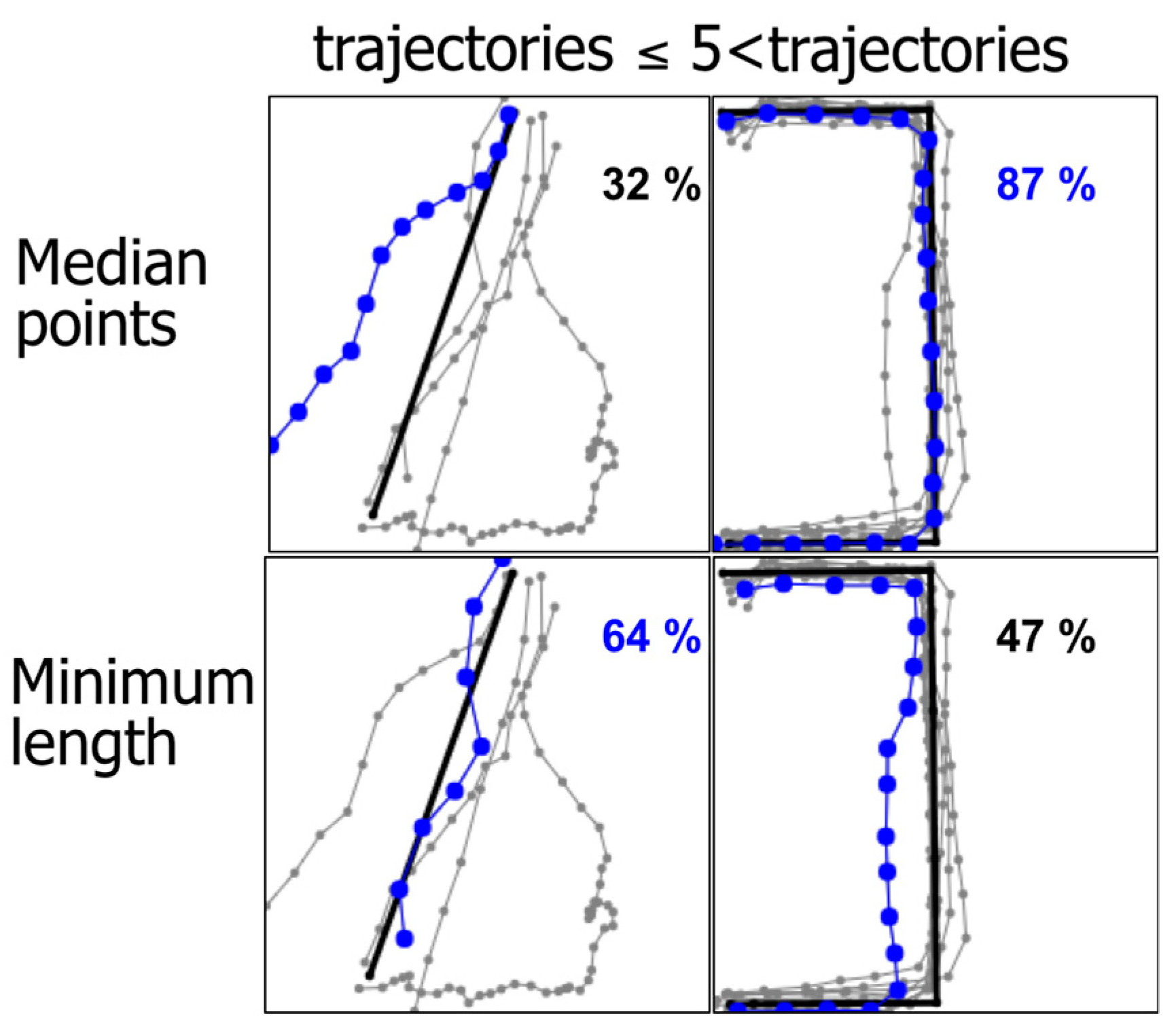
As a backup strategy, we select one of the input trajectories to represent the segment. To save computing time, we calculate the number of points in the trajectories and select the trajectory with the median number, as shown in Algorithm 3. We also considered the alternative strategy used in [8,9], which selects the trajectory with the shortest path length. It can sometimes work better, especially when there are only a few trajectories in the set, but it has problems when there are more trajectories in the set, see Figure 8. For simplicity, we stick to the median points strategy.
| Algorithm 3 (RapSeg-A): CurveSegment (X): |
| 1: Input: GPS trajectories: X 2: Output: representative: Y 3: FOR every trajectory Xi: 4: Ni ← Calculate the number of points in Xi; 5: j ← Select the trajectory with median value of all Nj; 6: Y = XXY; |
3.4. Curvy Model B: Medoid
Although the previous model works better than random guess, it is somewhat naïve. We therefore consider Medoid as a more solid alternative. Medoid is defined as the sample whose total distance to all other samples is minimal, shown in Equation (2). This can also be applied to the segment averaging problem if we define suitable distance function between the GPS trajectories, as shown in Algorithm 4. We use Hausdorff [12] as it is invariant to the travel distance and produces competitive results. Potentially better choices could be found in [11], but as Medoid is not the main strategy, we settle with the Hausdorff distance.
| Algorithm 4 (RapSeg-B): CurveSegment (X): |
| 1: Input: GPS trajectories: X 2: Output: representative: Y 3: j ← find the medoid from X via Eq. (2) 4: Y = Xj; |
In the context of GPS trajectories, we define Medoid as the input sequence xj that minimizes the following function.
The downside of the Medoid is its higher time complexity. Assuming that there are k trajectories to consider, each having at most n points, the time complexity of single Hausdorff computation takes O(n2), and therefore the total time complexity of finding the Medoid is O(k2n2). It is possible to use faster distance measures like Euclidean and Fast-DTW [13], but issues like having trajectories of different lengths and different point orders can have unwanted effects. In addition, linking components from multiple libraries can easily cancel the effect of an otherwise good idea—as also happened in [8]. We, therefore, settle here with the standard Hausdorff function:
where A and B are the two trajectories and dist is the Euclidean distance between two points.
3.5. Curvy Model C: Divide-and-Conquer
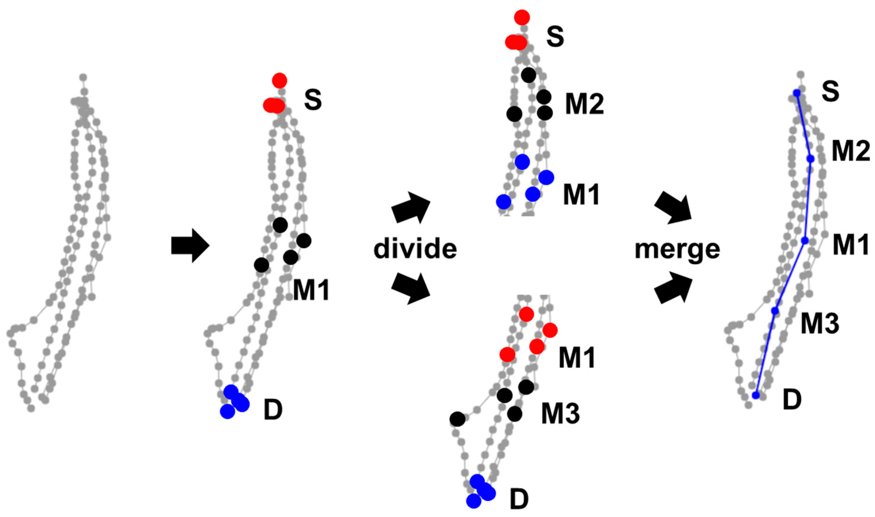
As the third alternative, we consider a simple divide-and-conquer approach as follows. If the descriptors indicate that the curvy model is applied, we divide the trajectories into two sub-segments at the median points (M) of each trajectory. Both sub-segments are then recursively processed by the same overall algorithm until the sub-segment reduces to the linear model, see Algorithm 5 and Figure 9.
| Algorithm 5 (RapSeg-C): CurveSegment (X, S, D, T): |
| 1: Input: GPS trajectories: X; threshold value: T 2: Output: representative: Y 3: M ← calculate the mean of the set of median points from each trajectory in X; 4: IF cos(∠SDM) ≤ T || cos(∠DSM) ≤ T: 5: X1, X2 ← cut each trajectory in X into two parts by the point at the median location; 6: ADD CurveSegment (X1, S, M, T) TO Y; 7: ADD CurveSegment (X2, M, D, T) TO Y; 8: RETURN Y 9: ELSE: 10: RETURN M; |
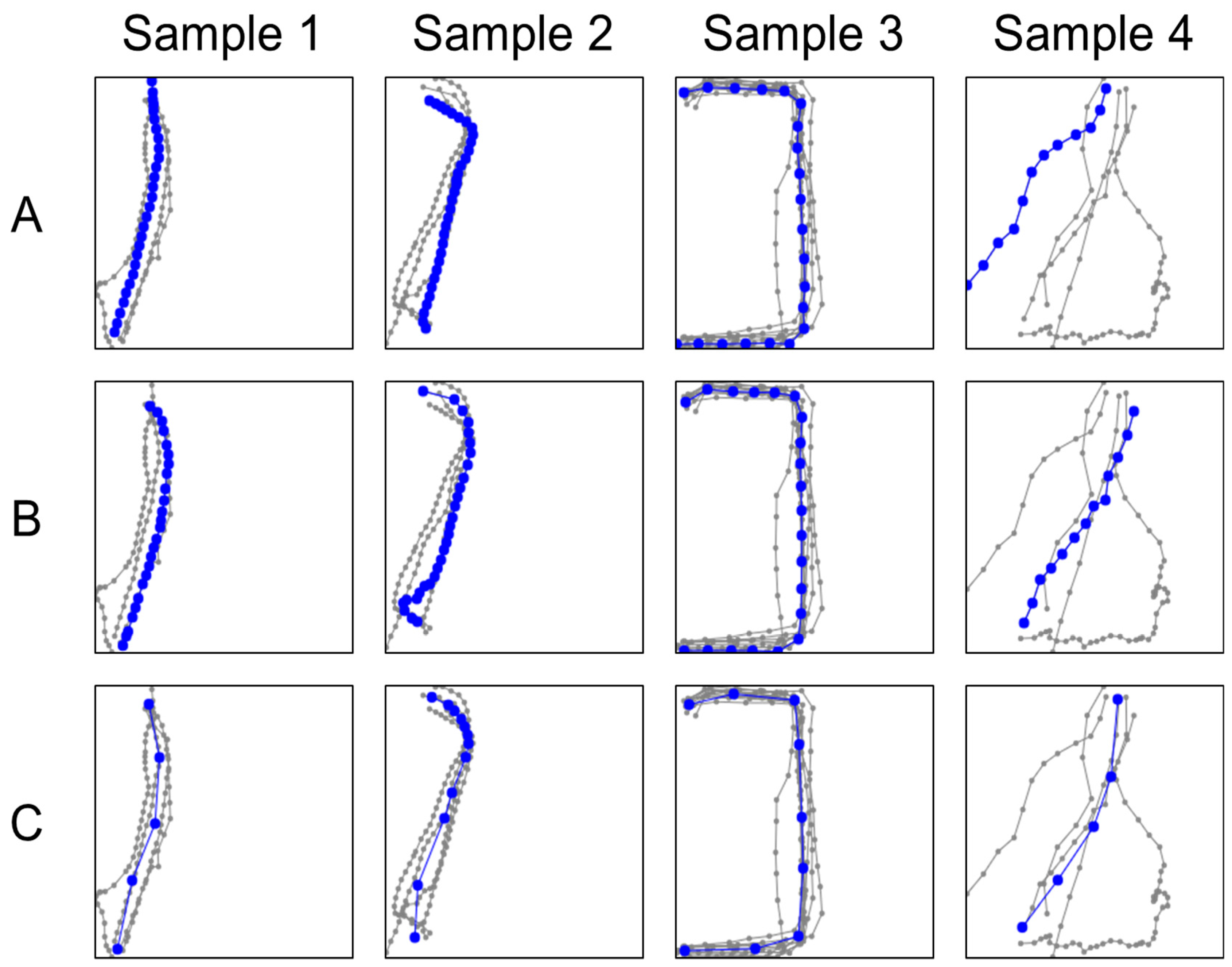
An example of this curvy model is shown in Figure 9. Figure 10 shows selected visual examples of all three variants. We can see that the variant C uses much fewer points than the other two variants. The number of points is also adapted to the situation; more points are allocated for the curvy parts of the segment, whereas the linear parts use only a few points to represent them.
3.6. Outlier Removal
The data contains many noisy trajectories. We, therefore, consider detecting and removing outliers as a preprocessing step. For simplicity, we apply an existing generic outlier detection method called Local outlier factor (LOF) [14], See Figure 11. It calculates the local density for every point as the distance to its furthest k nearest neighbor. Points having a significantly lower density than their neighbors, are more likely to be outliers. The outlierness of a point is the ratio of its density relative to the density of its neighbors. We apply LOF separately to the source and destination sets and detect the top 10% of the outlier points. To be safe, a trajectory is excluded if either its start or end point is detected as an outlier.
We smooth the effect of the outlier removal as follows. We calculate the descriptors (S, M, D) for the set both with (variant 1) and without (variant 2) outlier removal as illustrated in Algorithm 6. The final descriptors are then weighted averages of the two alternatives. We experimentally select the weights as a = 0.016, b = 0.600, and c = 0.510, which are optimized for the training dataset, see Section 4.
| Algorithm 6: Embedding (variant 1, variant 2) |
| 1: a, b, c = 0.016, 0.600, 0.510; 2: IF SIZE (variant 2) > 3: 3: RETURN variant 2; 4: ELSE: 5: S1, M1, D1 ← variant 1; 6: S2, M2, D2 ← variant 2; 7: IF SIZE(M2) == 0://M2 is empty 8: S = 2 * a * S1 +(1 + a) * S2; 9: D = 2 * a * D1 + (1 + a) * D2; 10: RETURN S, D; 11: ELSE: 12: RETURN S2, (b* M2 + (1 − b) * (c * S2 + (1 − c) * D2)), D2; |
3.7. Time Complexity
The time complexity of the method is summarized in Table 1. Considering the number of trajectories in the set k and the maximum number of points of a trajectory n, RapSeg-A takes O(k) per set. RapSeg-B takes O(n2k2), as it has the calculation of Medoid as the bottleneck. The actual processing time, therefore, depends on how many sets are processed by the curvy model. In our case, most sets are processed using the linear model (p = 93% for training data; p = 95% for test data), so this method is not as slow as it might first look. RapSeg-C takes O(Tk), where T is the number of times; we need to calculate M. In our case, T = 4.00 for training data and T = 4.33 for test data, on average. In the worst case, T can theoretically equal to n, in the case where every point in the curve is a turning point. In summary, RapSeg-A is the fastest, and RapSeg-B is the slowest.
4. Experiments
We use the datasets described in (http://cs.uef.fi/sipu/segments) [4]. The data include intersections taken from the open street map (OSM) and trajectories between those intersections, selected from four different data collections: Joensuu 2015 [11], Chicago [15], Berlin [16], and Athens [16]. Ground truth segments are also included as obtained from OSM. The evaluation is done by comparing the resulting average segments against the ground truth. The sets were grouped together and then randomly divided into 10% for training (100 sets) and 90% for testing (901 sets). There is a total of 10,480 trajectories consisting of 90,231 points. More details of the data extraction are available in [4].
For evaluating the accuracy of the segments, we use hierarchical cell-based similarity measure (HC-SIM) as proposed in [4]. It extends C-SIM measure (http://cs.uef.fi/mopsi/routes/grid) [11] to multiple zoom levels. C-SIM uses a grid of 25 × 25 m and counts how many cells the resulting segment average share with the ground truth segments from OSM relative to the total number of cells they occupy. HC-SIM uses six layers with the following grid sizes, 25 × 25 m, 50 × 50 m, 100 × 100 m, 200 × 200 m, 400 × 400 m 800 × 800 m. In case of the [0, 1] scale, the following sizes are used, 0.5%, 1%, 2%, 4%, 8%, 16%.
Results
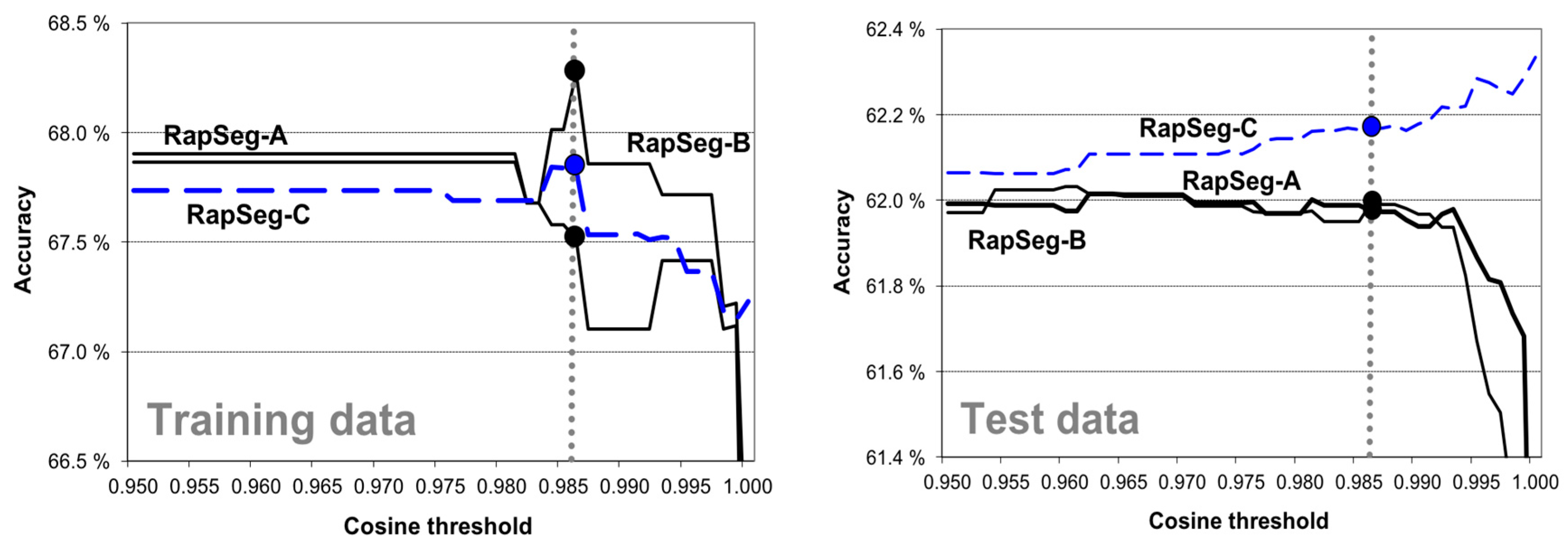
The effect of the threshold is shown in Figure 12. The results show that we can achieve good results even with the linear model. For example, RapSeg-A reaches 62.0% even without the curvy model. We set the threshold to 0.986 based on the training, as the performance seems to peek at that point. RapSeg-C reaches the best performance of 62.2%. If the threshold was increased further, the maximum performance of 62.3% could have been reached. Most of the performance is achieved already by the linear model, which indicates unbalance of the line and curve shapes in the dataset.
The effect of outlier removal is shown in Table 2. It clearly improves the performance with the training data, and the smoothed variant is always better than the full outlier removal as such. However, the results do not generalize to the test data, and the best results are reached by RapSeg-A and RapSeg-C without any outlier removal step at all. We, therefore, drop the outlier removal from the final method completely.
Comparison of the RapSeg method (without the outlier removal) is compared against existing techniques in Table 3. All variants outperform the existing methods on accuracy, processing time and the number of points. In other words, RapSeg does not only provide more accurate approximation of the segment but it also saves processing time. The closest competitor in terms of accuracy is the method by Marteau [17].
The performance of the different curve models is compared in Table 4. We can see that RapSeg-A has the best performance of length and processing time, while RapSeg-C has the best performance on accuracy and the number of points. The reason for the oversample of the other variants is the use of median/medoid, which use the original points as such without any attempt to reduce their amount.
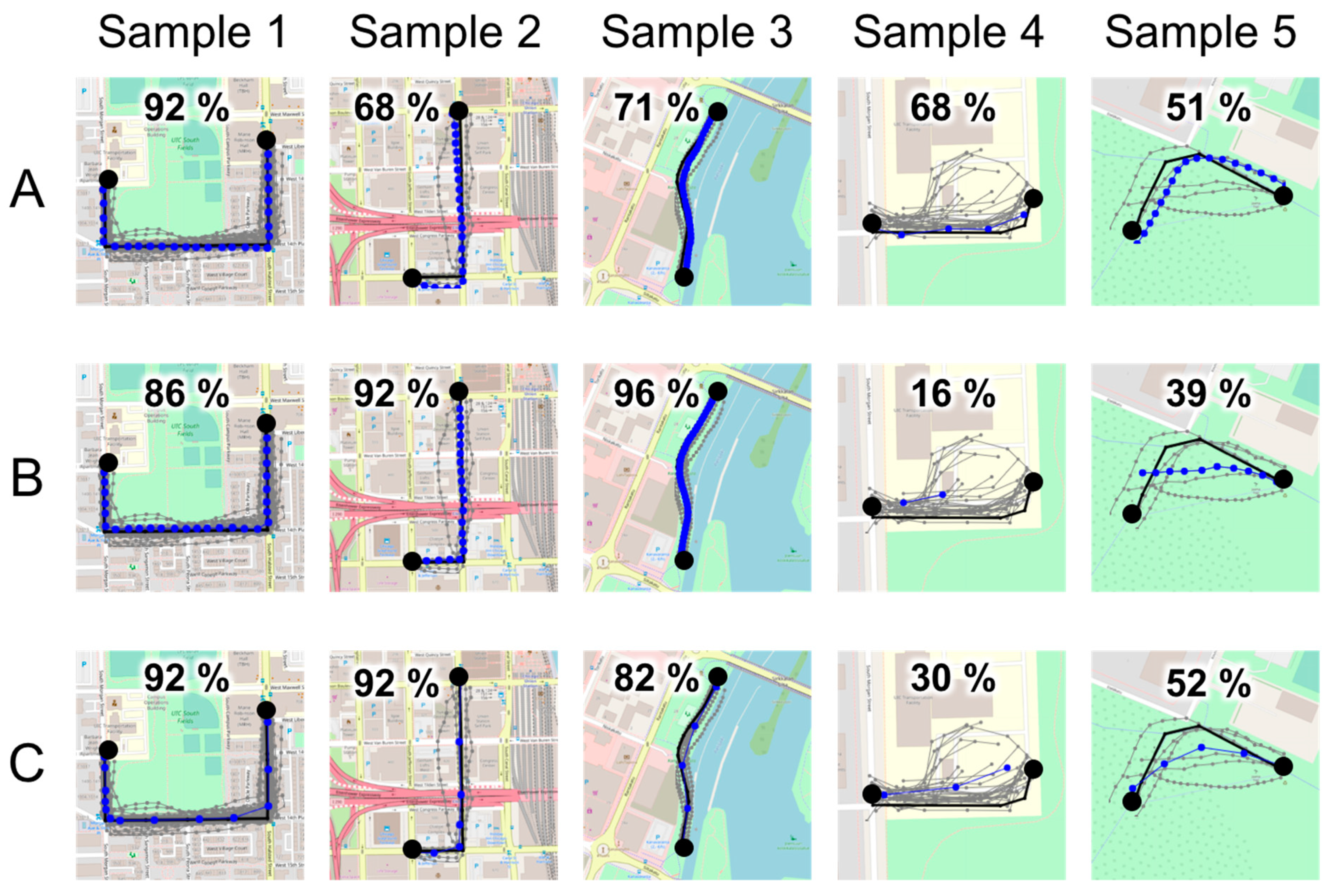
Their main difference between the variants is their processing time; RapSeg-B takes 5 times longer than RapSeg-A (0.59s vs. 3.39s), whereas RapSeg–C is almost as efficient (0.56s vs. 0.67s). From the visual examples in Figure 13, we can see that all methods provide satisfactory results whereas RapSeg-A appears to be more robust on noise.
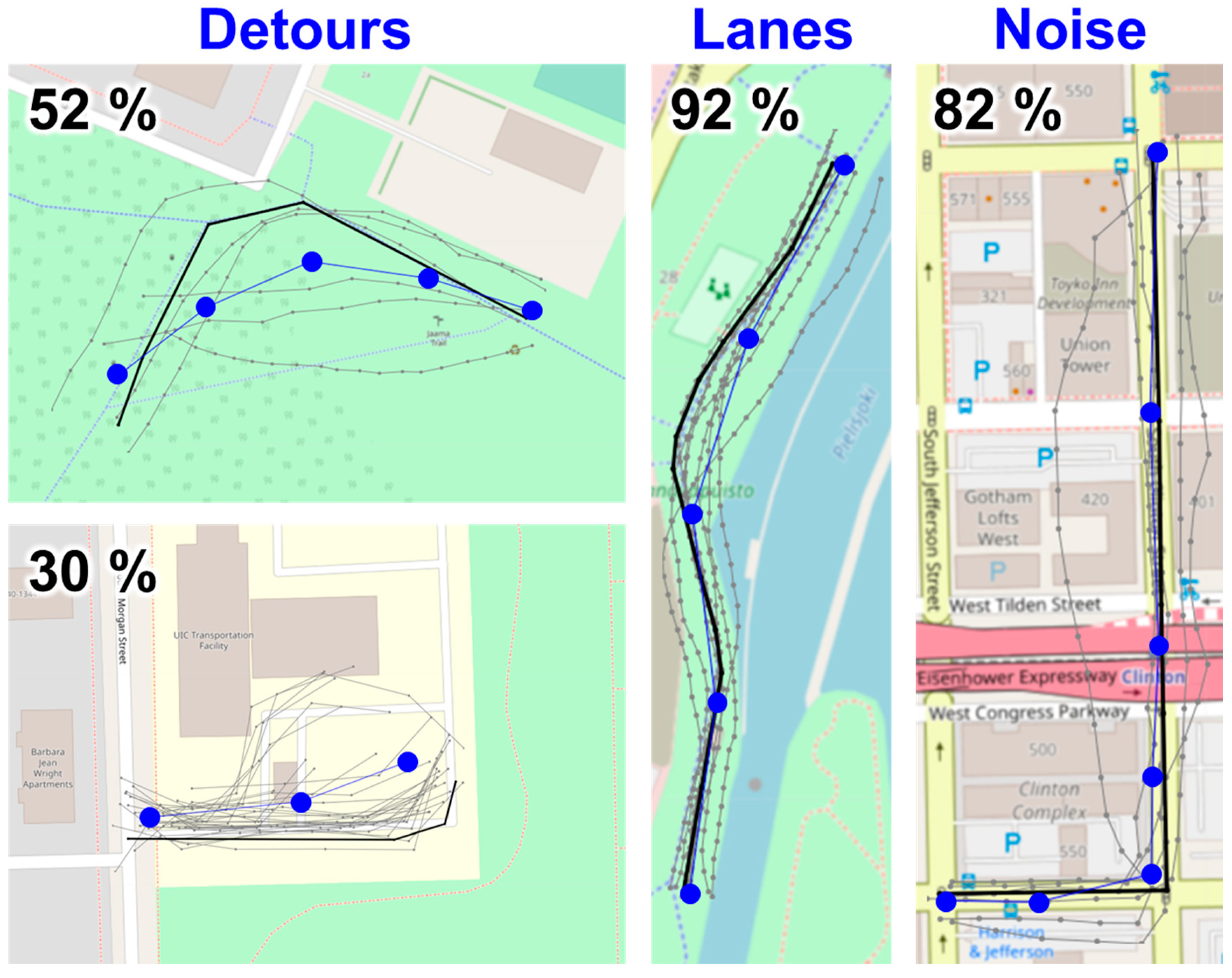
The zoomed examples in Figure 14 demonstrate some issues that could be improved further. First, if the extracted data contain multiple lanes then the averaging might not be accurate enough. In segment averaging, such issues are ignored, and we assume that lane extraction is already done during the data preparation. Second, the segment might also include detours. The top, leftmost example includes shortcut used in summer, whereas in winter, it is part of the crossing skiing track and not used by pedestrians. Similar detour exists in the example below where the campus bus usually follows the southern road to the parking lot, but occasionally takes the longer detour northside of the small building. Third, the bicycle track near the river is partly extended by the nearby boat pier, which partially follows the bicycle track in parallel. As a result, the average segment can be slightly deviated towards the river. Fourth, in the case of GPS noise caused by tall buildings, the segment deviates away from the buildings.
Further analysis by calculating Spearman correlation showed that the performance of RapSeg (all variants) correlates with the number of points (0.19–0.34) and with the number of trajectories (0.22–0.25). A positive correlation is expected, as more samples are expected to provide a better chance to derive the correct segment from the data. On the testing data, a negative correlation was observed between the performance and the variance (calculated using Hausdorff) between the trajectories in the set (−0.25). This is also as expected because it should be easier to find the correct segment average for a set with tighter packed trajectories. However, there is no correlation on the training set (0.06 Spearman correlation), which may be because the training set is smaller and populated by many sets containing only a few sample trajectories, which can skew the numbers.
5. Conclusions
Three fast segment averaging methods were proposed to handle complex curve segments. The two simple methods use linear model as the baseline and either median or medoid as the backup plan when linear model does not work well enough. The third method uses more complex divide-and-conquer technique to divide the problem into sub-problems.
The results showed that the simplest variant (RapSeg-A) achieves similarly good accuracy as the more complex variant (RapSeg-C): 62.0% vs. 62.2%. All methods are fast, simple to implement, and do not suffer serious oversampling. The processing time of RapSeg-A is an order of magnitude faster (12 s) than the comparative methods: Medoid (1 h), Marteau (30 min), and CellNet (49 s).
Author Contributions
The ideas and implementation of the algorithms originated from J.Y. and developed jointly by all authors. R.M.-I. and J.Y. conducted the experiments. Illustrations were prepared jointly by all authors. P.F. was the principal author wringing the paper.
Funding
This research received no external funding.
Acknowledgments
We would like to thank Jiawei Yang for his financial support from the Faculty of Science and Forestry.
Conflicts of Interest
The authors declare no conflicts of interest.
References
- Hautamäki, V.; Nykänen, P.; Fränti, P. Time-series clustering by approximate prototypes. In Proceedings of the International Conference on Pattern Recognition, Tampa, FL, USA, 8–11 December 2008; pp. 1–4. [Google Scholar]
- Brill, M.; Fluschnik, T.; Froese, V.; Jain, B.; Niedermeier, R.; Schultz, D. Exact mean computation in dynamic time warping spaces. Data Min. Knowl. Discov. 2019, 33, 252–291. [Google Scholar] [CrossRef]
- Bulteau, L.; Froese, V.; Niedermeier, R. Tight hardness results for consensus problems on circular strings. arXiv 2019, arXiv:1804.02854-v4. [Google Scholar]
- Fränti, P.; Mariescu-Istodor, R. Averaging GPS segments challenge 2019. 2019; Manuscript (under preparation). [Google Scholar]
- Wagstaff, K.; Cardie, C.; Rogers, S.; Schrödl, S. Constrained k-means clustering with background knowledge. In Proceedings of the International Conference on Machine Learning (ICML’01), San Francisco, CA, USA, 28 June–1 July 2001; pp. 577–584. [Google Scholar]
- Schroedl, S.; Wagstaff, K.; Rogers, S.; Langley, P.; Wilson, C. Mining GPS traces for map refinement. Data Min. Knowl. Discov. 2004, 9, 59–87. [Google Scholar] [CrossRef]
- Piegl, L.; Tiller, W. The NURBS Book, 2nd ed.; Springer: Berlin/Heidelberg, Germany, 1997. [Google Scholar]
- Mariescu-Istodor, R.; Fränti, P. Cellnet: Inferring road networks from GPS trajectories. ACM Trans. Spat. Algorithms Syst. 2018, 4, 8. [Google Scholar] [CrossRef]
- Fathi, A.; Krumm, J. Detecting road intersections from GPS traces. In Proceedings of the International Conference on Geographic Information Science, Zurich, Switzerland, 14–17 September 2010; pp. 56–69. [Google Scholar]
- Marteau, P.-F. Times series averaging and denoising from a probabilistic perspective on time-elastic kernels. Int. J. Appl. Math. Comput. Sci. 2019, 29, 375–392. [Google Scholar] [CrossRef]
- Mariescu-Istodor, R.; Fränti, P. Grid-based method for GPS route analysis for retrieval. ACM Trans. Spat. Algorithms Syst. 2017, 3, 8. [Google Scholar] [CrossRef]
- Rockafellar, T.R.; Wets, R.J.-B. Variational Analysis; Springer: Berlin/Heidelberg, Germany, 2009; Volume 317. [Google Scholar]
- Salvador, S.; Chan, P. Toward accurate dynamic time warping in linear time and space. In Proceedings of the ACM International Conference on Knowledge Discovery and Data Mining Workshop on Mining Temporal and Sequential Data, San Jose, CA, USA, 12–15 August 2007; pp. 70–80. [Google Scholar]
- Breunig, M.M.; Kriegel, H.; Ng, R.T.; Sander, J. LOF: Identifying density-based local outliers. In Proceedings of the ACM SIGMOD International Conference on MANAGEMENT of Data, Dallas, TX, USA, 15–18 May 2000; Volume 29, pp. 93–104. [Google Scholar]
- Biagioni, T.; Eriksson, J. Inferring road maps from global positioning system traces: Survey and comparative evaluation. Transp. Res. Rec. J. Transp. Res. Board 2012, 2291, 61–71. [Google Scholar] [CrossRef]
- Ahmed, M.; Karagiorgou, S.; Pfoser, D.; Wenk, C. A comparison and evaluation of map construction algorithms. GeoInformatica 2015, 19, 601–632. [Google Scholar] [CrossRef]
- Marteau, P.-F. Estimating road segments using kernelized averaging of GPS trajectories. Appl. Sci. 2019, 9, 2736. [Google Scholar] [CrossRef] [Green Version]
Figure 1.
Averaging a set of global positioning system (GPS) trajectories is needed in road network extraction (above) and clustering of GPS trajectories (below).
Figure 1.
Averaging a set of global positioning system (GPS) trajectories is needed in road network extraction (above) and clustering of GPS trajectories (below).

Figure 2.
Generic diagram of most existing methods for segment averaging.

Figure 3.
Sketch of the proposed solution: trajectories are analyzed based on three descriptors: start (S), middle (M), and destination (D). The input trajectories are colored by gray and the predicted average segment as blue.
Figure 3.
Sketch of the proposed solution: trajectories are analyzed based on three descriptors: start (S), middle (M), and destination (D). The input trajectories are colored by gray and the predicted average segment as blue.

Figure 4.
The general structure of the three methods.

Figure 5.
Flow diagram of selecting the three descriptors.

Figure 6.
Examples of descriptors. The red numbers are the minimum of the cos(∠SDM) and cos(∠DSM) values.
Figure 6.
Examples of descriptors. The red numbers are the minimum of the cos(∠SDM) and cos(∠DSM) values.

Figure 7.
Examples of applying the linear model.

Figure 8.
Examples of curved sets. The trajectories of minimum length and the median number of points are considered as representatives.
Figure 8.
Examples of curved sets. The trajectories of minimum length and the median number of points are considered as representatives.

Figure 9.
Examples of divide-and-conquer (RapSeg-C) approach for handling the curvy model.

Figure 10.
Examples of the three methods for handling the curvy model on four distinct samples.

Figure 11.
Outlier removal.

Figure 12.
Effect of the threshold: the higher the value, the more often the curvy model is used.

Figure 13.
Visualizations of the three methods for handling the curvy model on sample trajectories (gray) from the test dataset. Solution is blue, ground truth is black, and the results are shown on top of OpenStreetMap.
Figure 13.
Visualizations of the three methods for handling the curvy model on sample trajectories (gray) from the test dataset. Solution is blue, ground truth is black, and the results are shown on top of OpenStreetMap.

Figure 14.
Zoomed-in visualizations of RapSeg-C for handling the curvy model. Sample trajectories (gray) and the solution (blue) are plotted on top of OpenStreetMap.
Figure 14.
Zoomed-in visualizations of RapSeg-C for handling the curvy model. Sample trajectories (gray) and the solution (blue) are plotted on top of OpenStreetMap.


Table 1.
The time complexity of the proposed methods.
| Step | Solution | Complexity | |
|---|---|---|---|
| Linear Segment | Endpoints | Table look-up | O(k) |
| K-means | Clustering | O(k) 1 | |
| Median points | Table look-up + average | O(k) | |
| Curve Segment | RapSeg-A: Median | Selection | O(k) |
| RapSeg-B: Medoid | Hausdorff | O(n2⋅k2) | |
| RapSeg-C: Divide-and-Conquer | Calculate M | O(T⋅k) |
1 Assuming 10 iterations of k-means with 2 clusters: 2⋅10⋅k = 20⋅k = O(k).
Table 2.
Effect of outlier removal on the three variants, evaluated by hierarchical cell-based similarity measure (HC-SIM) accuracy.
Table 2.
Effect of outlier removal on the three variants, evaluated by hierarchical cell-based similarity measure (HC-SIM) accuracy.
| Outlier Removal | RapSeg-A | RapSeg-B | RapSeg-C | |
|---|---|---|---|---|
| Train | --- | 67.4% | 68.3% | 67.9% |
| Smoothed | 69.4% | 70.2% | 69.5% | |
| Full | 69.0% | 69.7% | 69.3% | |
| Test | --- | 62.0% | 61.9% | 62.2% |
| Smoothed | 61.8% | 61.9% | 62.0% | |
| Full | 61.3% | 61.4% | 61.5% |
Table 3.
Comparison of the methods, as evaluated by HC-SIM accuracy. Length and points are given relative to the corresponding numbers in the ground truth; therefore, 100% denotes the expected result.
Table 3.
Comparison of the methods, as evaluated by HC-SIM accuracy. Length and points are given relative to the corresponding numbers in the ground truth; therefore, 100% denotes the expected result.
| Method | HC-SIM | Length | Points | Time |
|---|---|---|---|---|
| Medoid [4] | 56.40% | 98% | 169% | ~1 h |
| CellNet [8] | 53.80% | 65% | 144% | 49 s |
| CellNet [8] | 61.20% | 96% | 144% | 48 s |
| Marteau [17] | 61.70% | 99% | 145% | 30 min |
| RapSeg-A | 62.00% | 99% | 81% | 12 s |
| RapSeg-B | 62.10% | 99% | 79% | 16 s |
| RapSeg-C | 62.20% | 99% | 77% | 13 s |
Table 4.
Comparison of the proposed methods on curve model, as evaluated by HC-SIM accuracy.
| Method | HC-SIM | Length | Points | Time |
|---|---|---|---|---|
| RapSeg-A | 53.05% | 99% | 194% | 0.59 s |
| RapSeg-B | 53.26% | 89% | 167% | 3.39 s |
| RapSeg-C | 55.53% | 95% | 120% | 0.67 s |
© 2019 by the authors. Licensee MDPI, Basel, Switzerland. This article is an open access article distributed under the terms and conditions of the Creative Commons Attribution (CC BY) license (http://creativecommons.org/licenses/by/4.0/).
Share and Cite
MDPI and ACS Style
Yang, J.; Mariescu-Istodor, R.; Fränti, P. Three Rapid Methods for Averaging GPS Segments. Appl. Sci. 2019, 9, 4899. https://0-doi-org.brum.beds.ac.uk/10.3390/app9224899
AMA Style
Yang J, Mariescu-Istodor R, Fränti P. Three Rapid Methods for Averaging GPS Segments. Applied Sciences. 2019; 9(22):4899. https://0-doi-org.brum.beds.ac.uk/10.3390/app9224899
Chicago/Turabian StyleYang, Jiawei, Radu Mariescu-Istodor, and Pasi Fränti. 2019. "Three Rapid Methods for Averaging GPS Segments" Applied Sciences 9, no. 22: 4899. https://0-doi-org.brum.beds.ac.uk/10.3390/app9224899
Note that from the first issue of 2016, this journal uses article numbers instead of page numbers. See further details here.