Advanced Constraints Management Strategy for Real-Time Optimization of Gas Turbine Engine Transient Performance


Propulsion Engineering Centre, School of Aerospace, Transport and Manufacturing, Cranfield University, Bedford, MK43 0AL, UK
*
Author to whom correspondence should be addressed.
Appl. Sci. 2019, 9(24), 5333; https://0-doi-org.brum.beds.ac.uk/10.3390/app9245333
Submission received: 14 October 2019
/
Revised: 28 November 2019
/
Accepted: 3 December 2019
/
Published: 6 December 2019
(This article belongs to the Special Issue Environmentally Friendly Gas Turbines)
Abstract
:Featured Application
The method that is described in this work can be used to assess the gas turbine engine performance under different control modes when the engine experiences transient operation. During this phase of operation, the engine needs to meet all the predefined constraints while it delivers the required performance efficiently and within its operating envelope.
Abstract
Motivated by the growing technology of control and data processing as well as the increasingly complex designs of the new generation of gas turbine engines, a fully automatic control strategy that is capable of dealing with different aspects of operational and safety considerations is required to be implemented on gas turbine engines. An advanced practical control mode satisfaction method for the entire operating envelope of gas turbine engines is proposed in this paper to achieve the optimal transient performance for the engine. A constraint management strategy is developed to generate different controller settings for short-range fighters as well as long-range intercontinental aircraft engines at different operating conditions by utilizing a model predictive control approach. Then, the designed controller is tuned and modified with respect to different realistic considerations including the practicality, physical limitations, system dynamics, and computational efforts. The simulation results from a verified two-spool turbofan engine model and controller show that the proposed method is capable of maneuverability and/or fuel economy optimization indices while satisfying all the predefined constraints successfully. Based on the parameters, natural frequencies, and dynamic behavior of the system, a set of optimized weighting factors for different engine parameters is also proposed to achieve the optimal and safe operation for the engine at different flight conditions. The paper demonstrates the effects of the prediction length and control horizon; adding new constraints on the computational effort and the controller performance are also discussed in detail to confirm the effectiveness and practicality of the proposed approach in developing a fully automatic optimized real-time controller for gas turbine engines.
1. Introduction
New designs and operations of gas turbine engines (GTEs) are increasingly complex where several constraints and control modes should be satisfied simultaneously to achieve a safe and optimal performance for the engine. To satisfy these requirements, current engine control systems are still mainly working with a min–max control philosophy. This strategy is known as a practical algorithm to satisfy all engine control modes simultaneously without any error and malfunction [1,2]. Results of the design and implementation of the min–max controller were presented within the Basic Research in Industrial Technologies for Europe-Europe/America (BRITE-EURAM) project OBIDICOTE (On Board Identification, Diagnosis and Control of gas Turbine Engines) and confirmed by all OBIDICOTE partners [3,4]. Therefore, this strategy is the most practical control method for gas turbine engines [5,6,7]. However, given the ambitious targets and severe limitations set by governments and organizations (e.g., the advisory council for aviation research and innovation in Europe has a target of a 75% reduction in CO2 emissions and a 90% reduction of NOx emissions by 2050 [8,9]), more robustness and flexibility is required for the next generation of GTEs control systems to adapt GTEs and aircraft performance to these standards and regulations.
So, the application of optimal control strategies for GTEs control modes satisfaction has been investigated extensively in recent years. Generally, the main feature of the optimal control theory is to use quadratic functions to solve the optimal control problems in complex systems. The linear quadratic regulator (LQR) is a typical case for solving general nonlinear optimal control problems that indicates the prospective design for the task of performance optimization [10]. This approach is used extensively for gas turbine engines controller design and optimization [11,12]. So, its basics and methodology are well understood, straightforward, and easy to implement. However, the shortcomings would be the iterative process required to deal with the problem, tuning the weighting matrix, and parameters handling [13,14,15]. An LQR is based on the receding horizon concept such that future outputs are predicted at every time step in order to minimize a global criterion/cost function. By estimating future outputs based on past outputs, the user is able to better regulate offset in tracking. Usually, the output horizon is infinite; otherwise, the user ends up with a model predictive controller. H_∞ and neural networks (NN) are also used for GTEs optimal control problems [16,17]. However, the main shortcomings of these approaches are the level of mathematical understanding needed to apply them successfully and the need for a reasonably good model of the system to be controlled.
Another optimal control theory is model predictive control (MPC). The main advantage of MPC is that it allows the current timeslot to be optimized while keeping future timeslots into account. MPC is working based on the idea of optimizing a finite time horizon, but only implementing the current timeslot and then optimizing again, repeatedly, thus differing from LQR [18]. This approach has also the ability to anticipate future events and can take control actions accordingly (PID (Proportional-Integral-Derivative) controllers do not have this predictive ability) [19]. On one hand, the prediction of future dynamic response in the MPC eliminates the iterative process as well as tuning the weighting matrix of LQR [20,21]. On the other hand, constraints to the engine parameters can be easily implemented to the MPC, which overcomes the problem of handling the parameters in LQR [22]. In comparison with H_∞ and NN, the MPC is simpler, which does not require an accurate dynamic model to initialize transient operation, and the engine constraints can be directly embedded in the control process [23,24]. Therefore, the constrained MPC method is the most suitable one for gas turbine transient process control and performance optimization, as it is fully capable of determining the control inputs and seeking the optimal route based on the prediction of engine dynamics to optimally satisfy all the engine constraints [25].
Consequently, it could be concluded that the next generation of GTE controllers must have:
- Higher flexibility to deal with control requirements and constraints at different flight and weather conditions. So, a lower coupling between the control channels has become a developing trend to improve the performance of classic scheduling technique (e.g., the min–max algorithm) [26].
- More robustness to cope with system uncertainties in order to adapt dynamics of the GTEs to the wide operating range requirements as well as varying working conditions.
This study contributes to the advanced constraint-based optimal control strategy development for the new generation of GTEs in the following ways:
- Practicality considerations: the control strategy and laws are designed based on realistic assumptions with respect to the implementation considerations, engine, and aircraft flight range, and designer requirements such as the maneuverability (to satisfy the control requirements of short-range aircraft engines) and fuel economy (to satisfy the long-range civil aero engines control requirements).
- System dynamics considerations: the dynamic behavior and frequency responses of different parameters such as the pressure, rotational speed, and thrust are considered in controller structure design, and a weighting factors regulation procedure is proposed to achieve a realistic optimal performance for the engine at different flight conditions.
- Implementation considerations: the implementation considerations are considered in two ways: from the simplicity of the controller structure to implement, and from the computational effort point of view to achieve the capability of real-time simulation and optimization.
- Constraints definition: a modular form of constraints definition and implementation will be considered in the control structure as well. The effects of adding more constraints to the system on performance behavior of the engine will be analyzed in detail.
- Controller characteristics: the effects of different controller parameters will be considered on the engine transient performance:
- ○
- Effects of weighting factor on maneuverability and fuel economy.
- ○
- Effects of system dynamics and parameters frequencies on the controller weighting factors selection.
- ○
- Effects of prediction length and control horizon on the controller performance.
- ○
- Effects of adding constraints on the system performance and computational efforts.
For this purpose, a thermodynamic model for a twin-spool turbofan engine, as a case study, is developed by using the inter-component volume (ICV) method to simulate the engine’s transient performance. In order to use the model in a real-time mode, a model identification approach is implemented to develop a recursive least square with varying stabilizing factor (RLS-SV) model for the engine. Then, a model predictive controller (MPC) is designed to deal with engine control modes, where the Lagrangian multipliers and Hildreth’s quadratic programming methods are utilized to deal with constraint inequalities and selecting the controller weighting values, respectively. The designed controller is tested in several operating conditions, and different criteria are discussed comprehensively followed by the conclusions.
2. The Engine Model
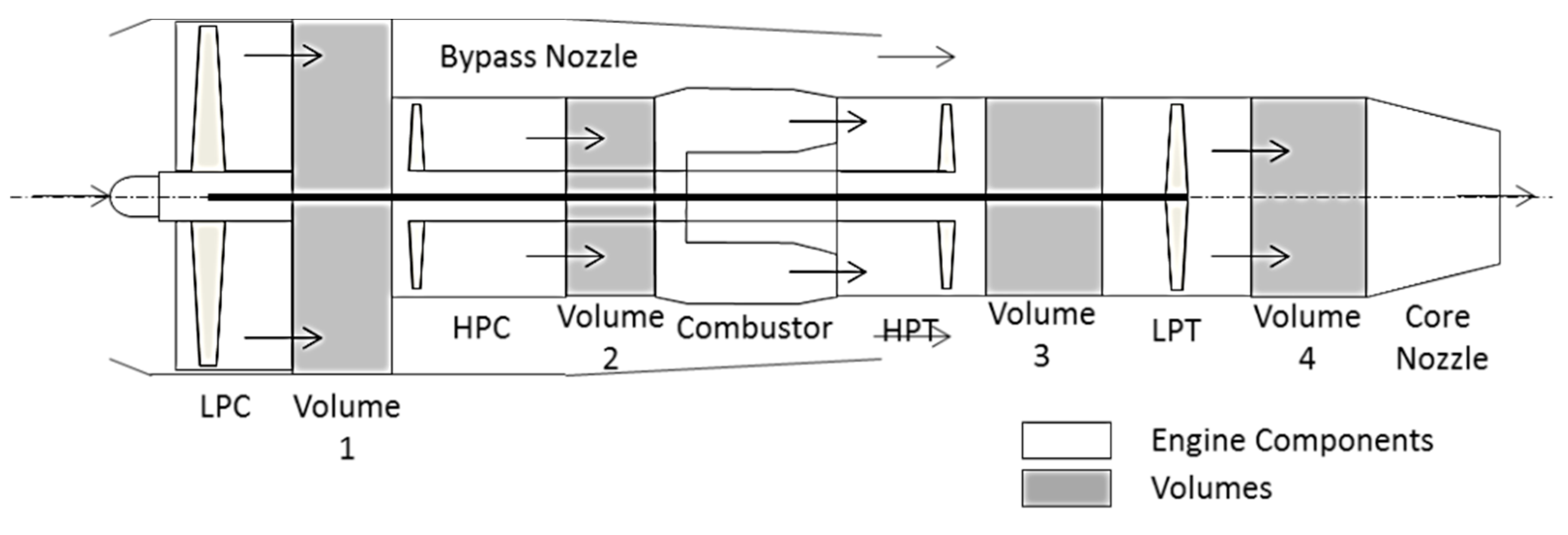
A twin-spool turbofan engine is used as a case study in this paper. The schematic sketch of the engine is shown in Figure 1 and the design point characteristics are shown in Table 1. A volume is added downstream of each turbomachinery component in order to simulate the flow propagation through the gas path (Figure 1), and the ICV method [27] is used to simulate the engine’s transient performance. The volume dynamics eliminate the discontinuity of engine parameters produced by the iterative and matching process in the components, and it simulates the flow propagation, especially on the pressure, temperature, and quantity change, from the inlet to the outlet of each component [28].
For the interest of overall performance, all turbomachinery components (compressors and turbines), as well as the combustor, are modeled individually considering the thermodynamic models. The estimation of the aerodynamic and thermodynamic parameters of these components has been conducted through energy conservation equations by the iterative process and matching the values from component maps [29,30]. The gas properties are estimated from the engine intake to exhaust by predicting the moisture calories [31]. The off-design performance has also been validated against Turbomatch code (a computing simulation platform developed by Cranfield University for performance predictions of gas turbine engines [32]).
The ICV method is realistic, since it includes an allowance for air/gas mass storage; thus, its predictions must be the more valid ones in comparison with other well-known methods such as constant mass flow (CMF) [27]. The ICV modeling technique brings the engine nonlinear transient performance closest to reality. However, to work with the MPC, a much simpler model is required to interpret the dynamics of the required engine parameters respective to the control input. Consequently, a discrete state-space model is identified in order to represent the engine dynamics in this paper.
3. Identification of the Engine Dynamics
The recursive least squares (RLS) algorithm is well known for tracking dynamic systems. Torres et al. [33] attempted to identify the dynamics of the gas turbine engine offline, mainly at steady states with stochastic signals. Arkov et al. [34] focused on real-time identification for transient operations and concluded that an engine system could be averaged to a time-invariant first- or second-order transfer function by the extended RLS. The tracking speed and accuracy for the RLS could be improved with a different design of forgetting factors. The effect of using a forgetting factor is to shift the estimating average toward the most recent data, such as that in the work by Paleologu et al. [35]. In this paper, a modified RLS algorithm (RLS with a varying stabilizing factor (RLS-SV)) is investigated for the online dynamic identification of gas turbine engines. The method is capable of updating itself to adapt to the change of engine dynamics due to the variation of engine transient levels and operating conditions.
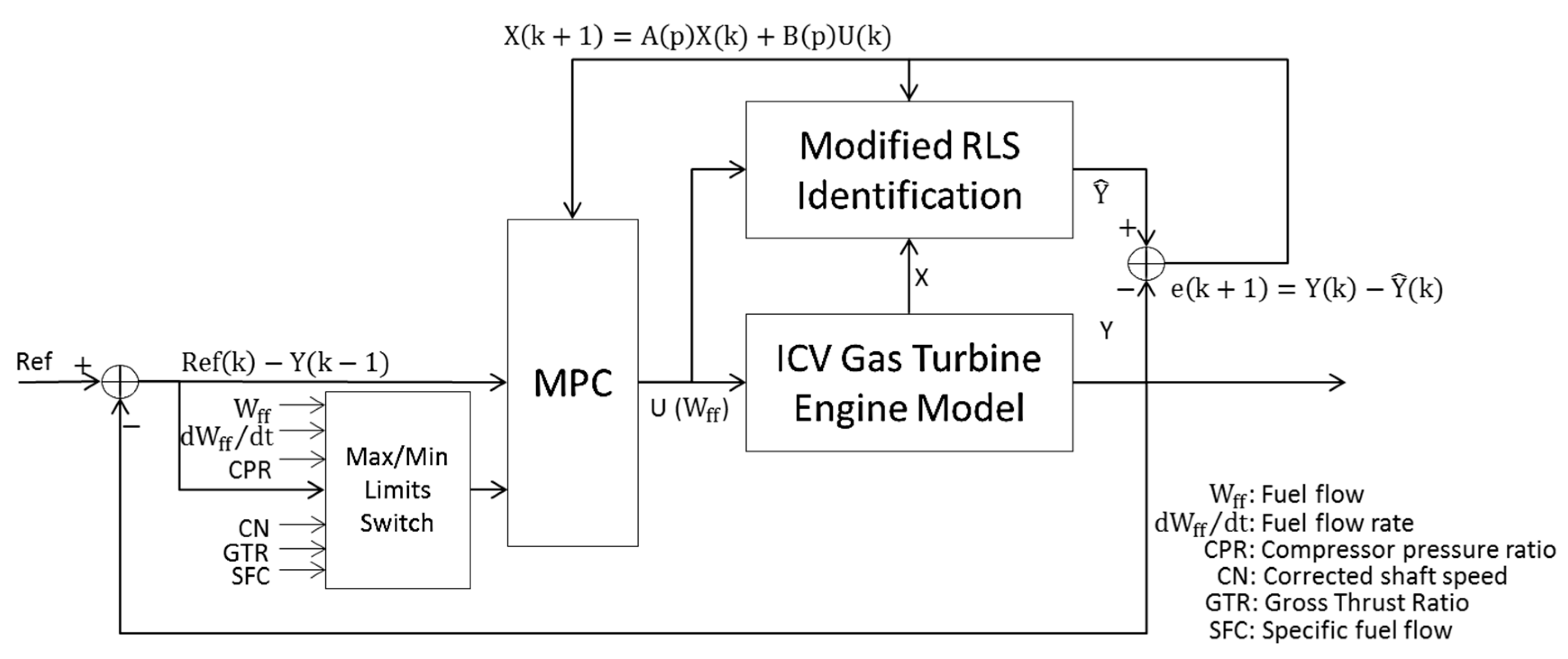
The main structure of the model and controller is shown in Figure 2. The modified RLS model is developed to track the detailed gas turbine engine model, and the ICV method is used to predict the transient behavior. The output of the model is imported to the MPC controller, where reference inputs and constraints are analyzed as well. The MPC controller calculates the optimized fuel flow at any instantaneous time for the engine. This control input will satisfy all engine control modes and constraints simultaneously while guaranteeing the optimized operation for the engine based on a predefined objective function.
A general format of the discrete state-space model is shown in Equation (1). The state matrix () contains state variables that are from engine parameters relative to the output variable including shaft speed, compressor pressure ratio, and thrust. The output matrix () is a subset of the state matrix. The input matrix (U) contains the control inputs and fuel flow, which controls the engine to fulfill the desired output. Moreover, A, B, and C are the system, input, and output matrices, respectively.
The coefficient matrices (A, B) in the state-space model are being identified and updated at each time step for adapting the nonlinear engine dynamics. If there are “m” number of engine state variables, and “n” number of engine input parameters, “A” is a square matrix with the dimensions of , and “B” has the dimensions of . The coefficient “C” is fixed because of the recursive requirement, and the output must be a subset of the states. The parametric matrix and the objective matrix become:
The error between the output measurement and the estimation is defined as:
Using the matrix inversion lemma (MIL), the reversion of the covariance matrix in RLS has been eliminated, and the determination of the covariance only requires the engine data from the previous time step as shown in Equation (4).
As mentioned earlier, a factor multiplies the covariance matrix of Equation (4) in order to shift the estimation average to the recent engine outputs. The state-space model can be more adaptive to the rapid change in engine performance, with an introduction of an adjustable term to the covariance, as shown in Equation (5):
The normalized factor µ (0 ≤ µ ≤ 1) acts as a forgetting factor for the reduction of recursive power. A new term added to the end of Equation (5) is an adjustable weight, which limits the growth of eigenvalues to the matrix within an acceptable range relative to the change in gradient of engine parameter values so that the sensitivity based on the gradient can be automatically adjusted between the engine steady and transient states [36]. The coefficients in Equation (1) are updated continuously in the objective matrix () as follows:
The process is repeated, and the estimated state-space model is being updated at each time step for the supplement to the controller.
4. Model Predictive Controller Design for Gas Turbine Engine
In general, the MPC algorithm predicts the change in the dependent variables of the modelled system that will be caused by changes in the independent variables. So, the MPC would operate on top of the discrete engine model as shown in Figure 2 [37]. The control decisions from the MPC are based on the linear predictions from the linear state-space model (Equation (1)), and the predictions are amended due to the updates of the state-space model by RLS-SV at each time interval. The prediction by the MPC is produced by the incremental state-space model, as shown in Equation (7). The incremental model uses discrete differences (∆U, ∆X) input and state parameters (U, X) from the state-space model.
where k is the time step. Replacing U and X by (∆U, ∆X), the state-space model shown in Equation (1) can be written in the following matrix form, as shown in Equation (8).
Due to the principle of the receding horizon utilized by the MPC, the output parameter must be a subset of the state matrix. The performance prediction is possible when the output of the state-space model, Equation (8), only involves the receded control inputs. The new coefficient and variable matrices in Equation (8) have replaced the original matrices in Equation (1). Nc and Np define a finite length of the control and prediction horizons of MPC, and the length (Np ≥ Nc) can be customized according to the engine configuration, parameters’ natural frequencies, and sampling time. The linear predictions based on Equation (8) can be expressed as:
The linear prediction for the outputs can be written as:
The predictions in Equation (10) can be re-written as matrix form:
To simplify the constants in Equation (11):
To optimize the engine transient performance, optimal control inputs should be achieved by minimizing the objective function, as shown in Equation (13), so that the predicted outputs (Y) can accurately reach the final control target (W) in the cost function:
The minimization of the cost function is obtained from the derivation of Equation (13) for the optimal control solution as follows:
That results in Equation (15):
“” is a weighting factor matrix to the future control inputs, which is used to restrict the amount of change in the control inputs to the plant. This matrix has the length of the prediction horizon (Np), and all of its parameters are chosen between 0 and 1. Each value in the matrix can be different depending on the system dynamics, the natural frequencies of the state and output parameters, and the control task. When the value is close to 0, the input is more responsive to the change of output. While for values closer to 1, more control weight is added, and a slower change of fuel flow rate is being supplied to the engine’s combustor, which is suitable for obtaining a smooth power transition.
The constraints required for the safe and optimal operation of the engine are defined in the form of Equation (16). These constraints are to limit the change rate of fuel flow, the shaft rotational speed, the compressor surge, and the turbine entry temperature.
For the convenience of computation, the constraint values are moved to the right-hand side of Equation (16), and the left side of the inequality becomes a unity. The result for the input parameters is shown by Equation (17), in which the constraints can be added to monitor the magnitudes and the rate of change. However, monitoring the output parameters (output (Y) parameters) requires substituting the prediction functions, as shown in Equation (12), to Equation (16), which gives Equation (18) followed by the same rearranging process as the input parameters.
Other engine parameters, such as the compressor pressure ratio, shaft speed, turbine entry temperature (TET), and Specific Fuel Consumption (SFC) to monitor the engine performance or engine health, can also be included in the Equation (18). The dynamics of the constrained parameters are also predicted linearly in the same way as the outputs, as shown in Equation (12). The right-hand side of Equation (18) is the difference between the outputs/constraints’ limits and the predicted values. Then, all the inequality equations for the input, output, and other engine parameters can be combined, as shown in Equation (19). For simplification, “M” is the identity matrix on the left-hand side of ∆U, and everything on the right-hand side of inequality can be simplified as “γ”:
M ∆U − γ ≤ 0.
Taking the derivative from Equation (13), plus the inequality term of Equation (19), the objective function could be rewritten in the form of Equation (20). This is a well-known form of the objective function that could be dealt with by Lagrange multipliers, which is a strategy for finding the local maxima and minima of a function. This function is subjected to equality constraints, (i.e., subject to the condition that one or more equations have to be satisfied exactly by the chosen values of the variables), to solve challenging constrained optimization problems [37]. The ranking factor “λ” is calculated according to the impact of engine constraints to their corresponding parameters. In Equation (20), the minimization process predicts the optimal control values to achieve the objective output in the shortest time, and the maximization process is to compensate the control values by the constraints from the most severe limit.
The optimal control solution of Equation (21) is taken from the derivative of Equation (20).
The maximum value of “λ” is selected through the Hildreth’s quadratic programming method, which ranks the constraints based on a level of urgency. Higher urgency produces a higher value of “λ” parameters. The optimal future control inputs are predicted through Equation (21). Only the first sample input from the sequence is used by the controller, although the optimal control plan has been predicted throughout the entire control horizon. The process is repeated for each sampling time step. When new data is available, the prediction by the constrained MPC will be updated.
Putting everything into a nutshell, it can be concluded that the numerical procedure and solution for the problem includes four main phases: modeling, control, constraints definition, and solution, as described in Table 2.
5. Implementation and Results
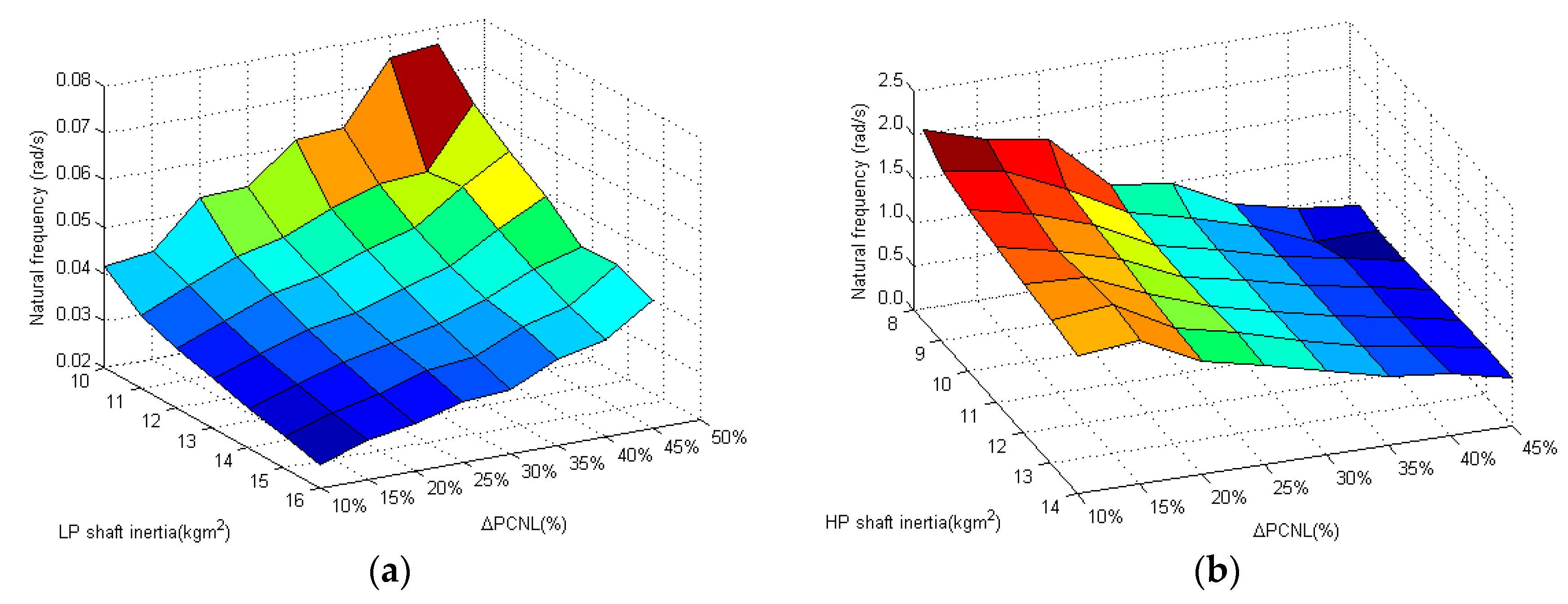
As discussed earlier, the combination of nonlinear characteristics from the components i.e., compressor, turbine and combustor, and variable gas properties contributes to the nonlinear engine performance. This nonlinearity can be noticed in Figure 3 from the frequency distribution through the parameters operating range. The frequency of the compressor pressure ratio changes due to the increment of shaft speed at different shaft inertias. Consequently, the conventional control design requires a control schedule at each operating point, and the control values are interpolated between the scheduled points. However, implementing the modified RLS, (Figure 2), allows the estimation of engine dynamics to adapt to the change of the nonlinear behavior of the modeled engine; then, the optimal transient performance can be obtained through the dynamic prediction according to the identified dynamic models by the MPC so that no control schedule is required.
A small sampling time (0.05 s) (20 Hz data) has been selected for the simulations to ensure the sustainable estimation of engine dynamics in the ICV method. In addition, with such a small sampling time, the control system does not require a nonlinear MPC design for operating the engine to its optimal performance. The dynamics of the selected engine parameters, such as compressor pressure ratio and relative rotational speed, are approximated as second-order functions due to the coupling between high- and low-pressure components and mechanical linkage. Therefore, estimating the speed of one shaft requires the inclusion of speed from the other shaft as a state variable to the state-space model. However, there is no definite technique for determining the order of dynamic functions. The selection of the model order is referred to the experimental results and the equations used in the ICV model [38,39].
In the designed control structure, the engine fuel flow (Wff) is the control input. The total gross thrust ratio (GTR), which is the ratio of the sum between the bypass gross thrust (GTbypass) and core gross thrust (GTcore) to 100% gross thrust at the design point (DP) is the output. However, as the thrust is not measurable in real-world applications, the engine rotational speed or engine pressure ratio could be used as the output as well. During transient operations, the high-pressure components are more likely to exceed their performance boundaries due to the relatively higher frequencies. As the example of high-pressure compressor pressure ratio (HPC-PR) in Figure 3b, the HP shaft speed has approximately a 25 times higher frequency than the LP shaft. The over-speed to the high-pressure shaft speed (CNH) and surge protection to the high-pressure compressor (HPC) are included for compressor protection. The turbine entry temperature (TET) is required to be monitored to prevent turbine overheating. Since the HP turbine is directly downstream of the combustor in Figure 2, the TET relates to the combustor outlet temperature (COT). According to the conservation of energy, Equation (22) calculates the value of COT involving the airflow as well as the fuel flow or fuel–air ratio (FAR), which simplifies the two parameters to one. Therefore, the FAR is also included in the estimated engine model as an additional state variable for the estimation of TET.
As an additional performance specification, the SFC value can be included to improve the engine fuel economy or to limit the emission. So, the final state-space model of Equation (1) can be rewritten in the form of Equation (23), with nine state variables, one control variable, and one output variable.
Table 2 shows the constraints boundaries, which have been implemented to this engine. The first seven constraints are designed for safety protection, and the last two constraints are designed for performance optimization. To set up the engine constraints, the constraint inequality equation can be written as Equation (24). The surge margin on a high-pressure compressor is approximated from a linear function from the high-pressure shaft speed. According to Table 3, “aHPC_max” is 9.5625, “bHPC_min” is −2.1096, “aHPC_min” is 3.0198, and “bHPC_min” is 0.0180, which are the constants for the surge margin.
The constraints in Equation (24) can be separated into factor and constant terms, as shown in Equation (25).
According to Equation (18), the constraint inequality function from Equation (25) can be written as Equation (26).
The simulation results of the designed controller are presented and discussed in detail in the following section.
5.1. Maneuverability and Fuel Economy
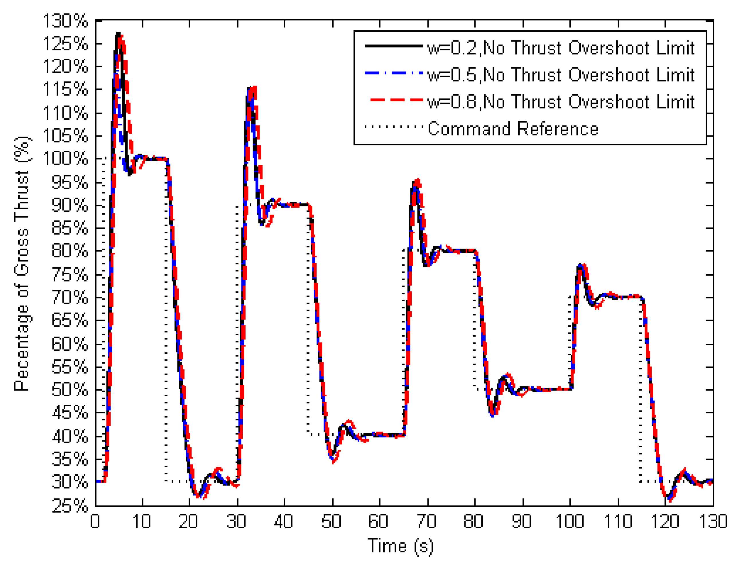
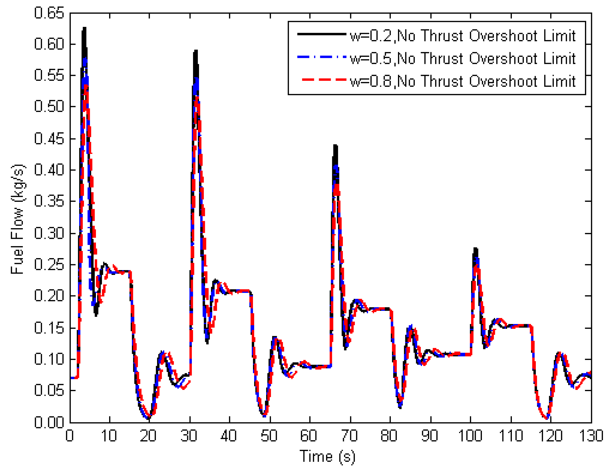
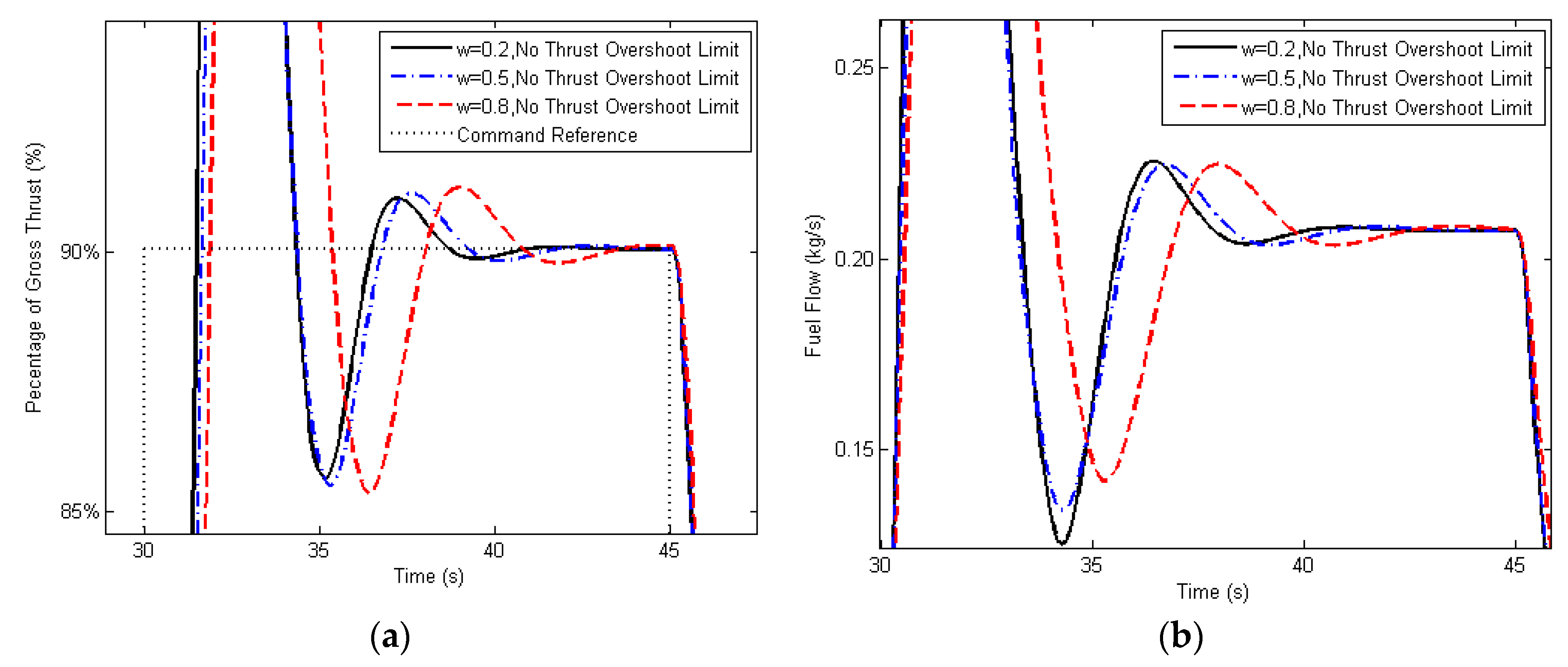
Different values for weighting factor “” in Equation (21) control the change of control input at each time step. The obtained results show as this value becomes closer to 0, a faster transient response can be obtained (Figure 4) with a larger amount of over-fueling (Figure 5). In other words, the smaller values for the weighting factor provide more violent control actions to the change of engine performance. In a close-up view, a slower transient response and a smaller amount of over-fueling are achieved by selecting larger values for the weighting factor (Figure 6). Too small values can reduce the control stability and increase the difficulty of limiting engine parameters within their constraints as well. However, the weighting factor value must be kept sufficiently small for the satisfaction of the time requirement (maximum 5 s) for the transient operations over the entire operating range according to the regulations [40]. In this case, a slightly smaller weighting factor (0.2) is selected for ensuring fast transient operations, and such a value still allows the MPC to constrain the engine parameters within their limits.
Consequently, smaller values for weighting factors enhance the maneuverability of the engine, which is suitable for short-range fighters’ control. However, the larger values for the weighting factor are associated with better fuel economy, which could be a priority in a civil-engine controller design procedure.
5.2. Effects of System Dynamics on the Controller Weighting Factor Selection
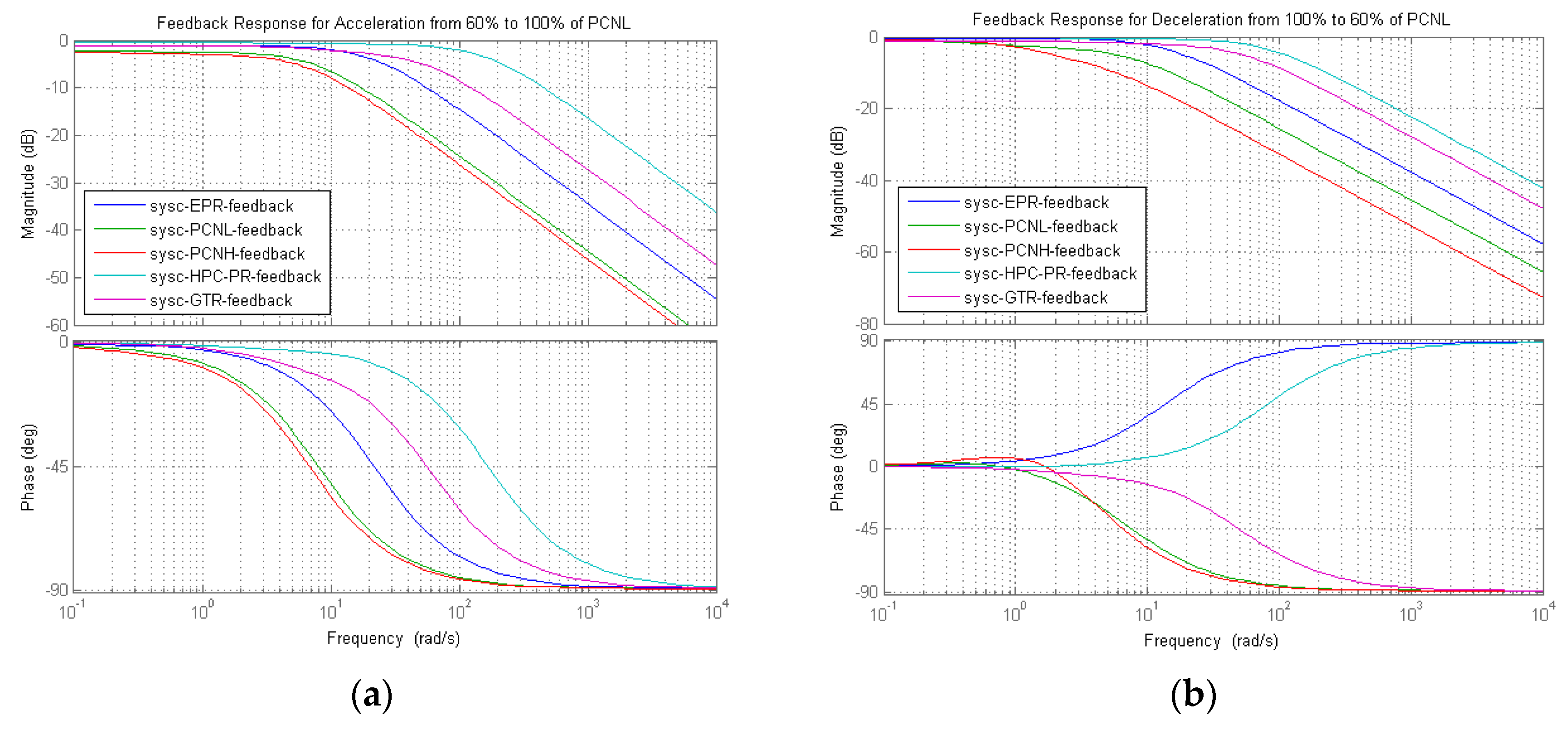
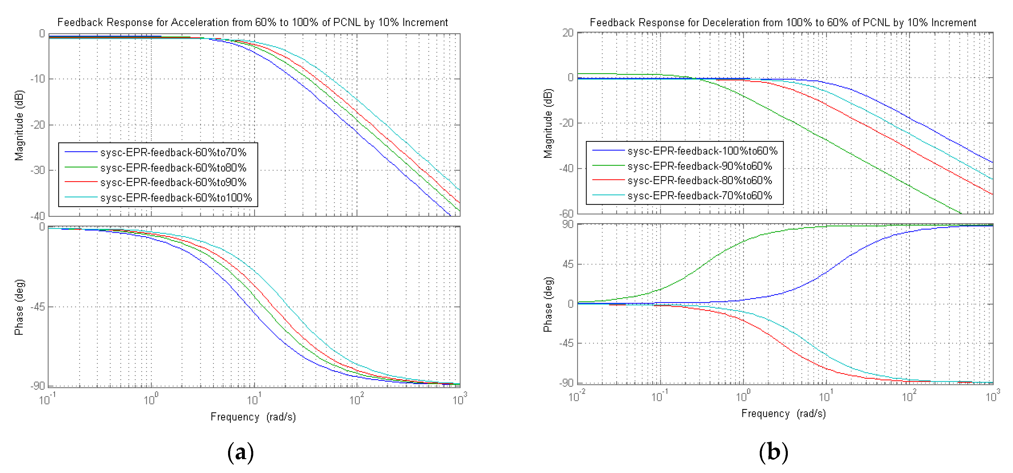
The selection of the weighting factor is also affected by different output parameters due to their different frequencies. Figure 7 shows the closed loop frequency response for the engine output parameters: gross thrust ratio (GTR), engine pressure ratio (EPR), percentage of relative rotational speed for a low-speed shaft (PCNL), percentage of relative rotational speed for high-speed shaft (PCNH), and HPC-PR during transient operation between 60% and 100% of PCNL. From this figure, all of these parameters have infinitive gain and phase margins. So, a relatively smaller weighting factor can be applied by the MPC for the parameters, which have a wider cut-off frequency. In this case, as shown in Figure 7, the order from the highest to the lowest frequency is HPC-PR, GTR, EPR, PCNL, and PCNH. In terms of the overall thrust delivery during transient operations, although HPC-PR has the fastest response, the time to the final steady state is determined by the low-pressure modules. This happens because the low-pressure modules deliver the biggest proportion of thrust, and in order to drive LPC, the high-pressure module was deliberately allowed to overspeed and have a higher percentage of overshoot in order to to allow the LP module to be quickly stabilized to the final steady state.
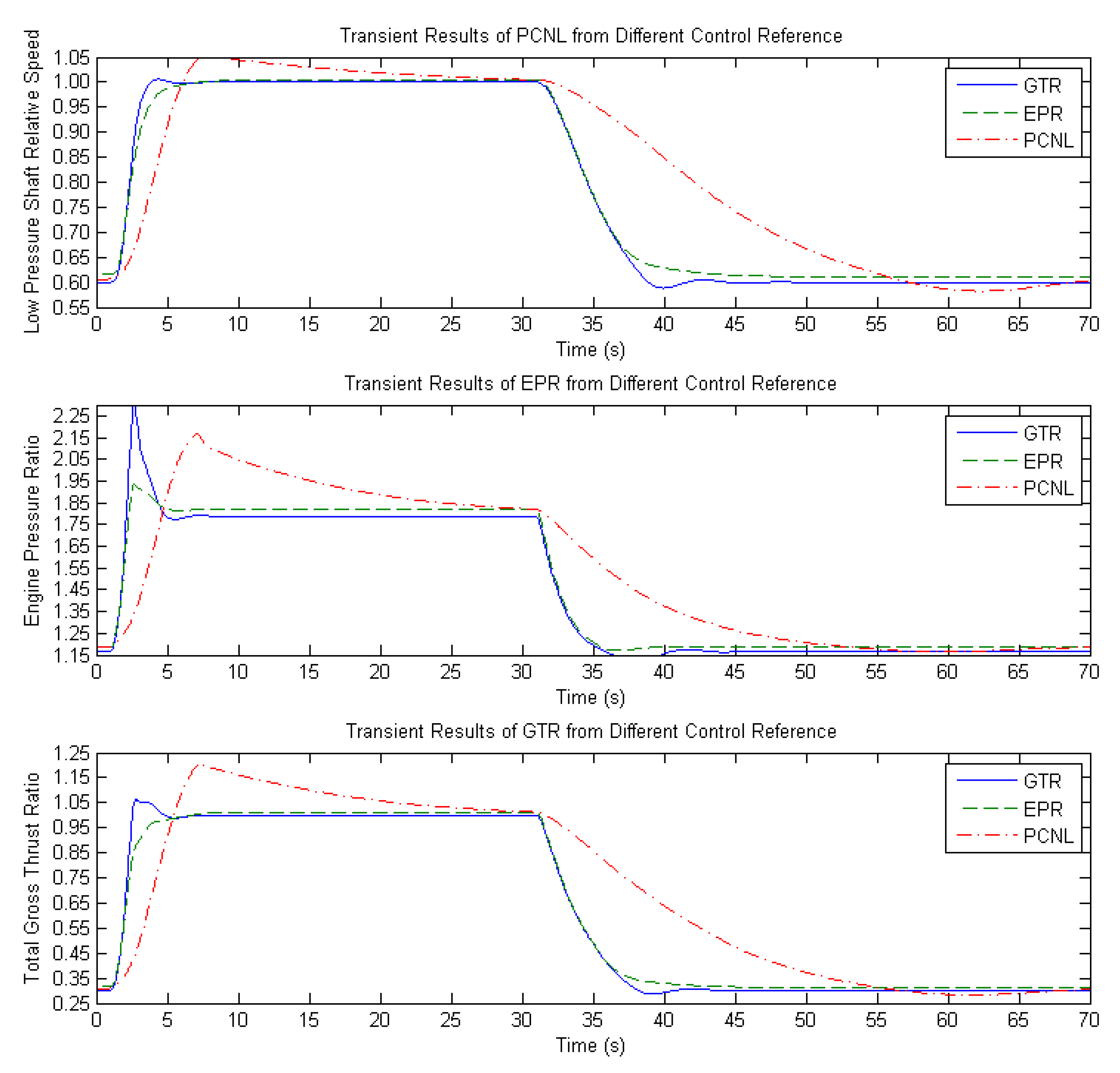
To match the transient response of GTR, EPR, and PCNL for the same transient operation in Figure 8, the weighting factor was chosen as 0.2 for GTR, 0.4 for EPR, and 0.6 for PCNL. Although a larger weighting factor has been set to PCNL for a slow response, PCNL was still containing the largest overshoot with the slowest response due to the coupling effect between the low and high-pressure modules and their inertia (Figure 9).
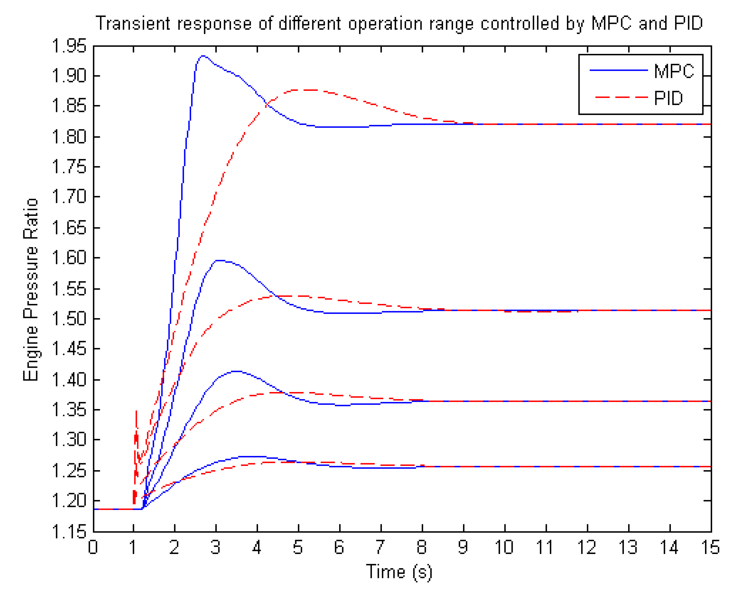
Figure 9 demonstrates the frequency response of closed-loop control to the EPR during transient operations with a different increment of PCNL from 60% to 100%. The results show that a higher frequency response corresponds to a larger range of transient operation. Due to frequency shift, using gain-scheduling method requires adjusting the control gains in order to adapt to the frequency shift when switching between different transient ranges for smooth operations and maintaining the amount of overshoot, such as the values shown in Table 4. Figure 10 shows the comparison results of transient operations under the control of MPC and scheduled PID. It can be seen that a smaller value of weighting factor with a consideration of engine constraints ensures the fastest, smooth, and safe transient response for the entire operating range.
5.3. Effects of Prediction Length and Control Horizon
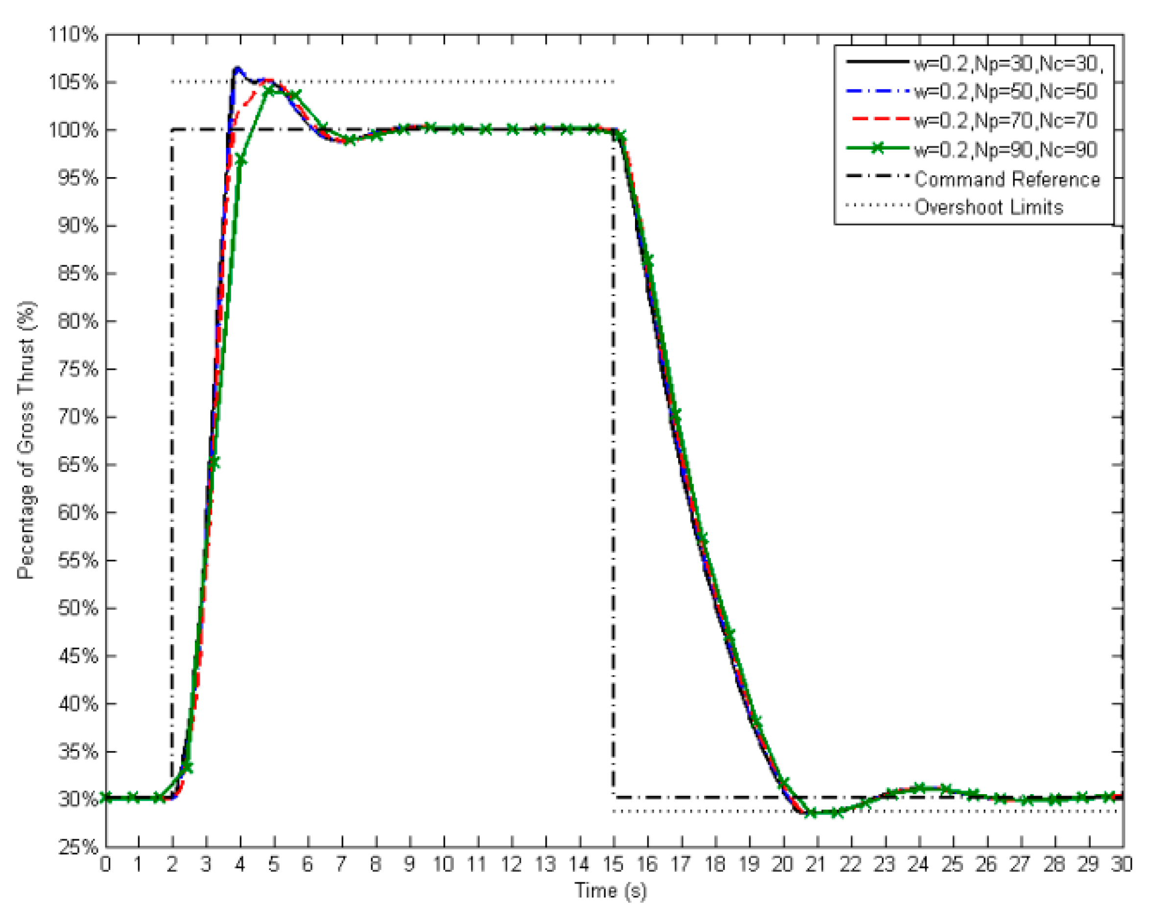
Longer prediction and control horizon allow the MPC to have a longer vision to anticipate the future of engine states. In accordance with the performance prediction, a fuel schedule can be planned so that the control action is applied in advance for the satisfaction of the transient time and constraints. Figure 11 shows the transient results controlled by MPC with different lengths of prediction and control horizon. Unlike the input constraints where the input parameter can be restricted directly, the control efforts cannot immediately result in the performance of state and output variables due to the lag of response. In addition, at certain operating circumstances, the control solution may not exist or is not feasible to satisfy all constraints simultaneously. Therefore, the constraints applied to the state and output variables in the state-space model are often implemented as “soft” conditions. The results given by MPC with 30 and 50 steps of prediction length are almost overlapped (Figure 11). Any horizon is set below 50 steps; the constraints, such as on the output (gross thrust ratio), cannot be kept within their limits (within 5% overshoot). Due to the input constraints in Table 2, the input of the fuel rate is limited, and the output cannot react and be penalized on time when the operating points are close to 105% of the final steady state during acceleration. In this contradictive situation, the MPC chooses to satisfy the input limit and compromise the output limit. As per the illustration, a longer horizon allows the MPC to detect the boundary conditions and prepare the penalized fuel flow earlier so that the running line can be kept within the threshold. However, a longer horizon also brings the consequence of the increase of rise- or fall-time. The increase of horizon length also increases the dimension of all the coefficient matrices in Equation (21) as well as the required computational effort. In the case demonstrated in Figure 11, one of the horizons is 90 steps with six constraints, (Table 2; ignoring the constraints of TET and SFC), and one output variable according to Equation (23). The dimension of matrix “F” in Equation (12) can be as large as at each sampling time. If a moderate horizon length (70 steps) is chosen, the controller is not only capable of allowing the transient operation to be completed within 5 s and within the limit the 5% overshoot, but also saves the computing memory by reducing 120 columns and rows (total elements) of matrix “F” ().
5.4. Effects of Defined Constraints on the Engine Behavior
It is also important to consider the effects of adding an additional constraint on the engine transient response and the computational efficiency. An additional engine constraint adds Np rows with Nc columns to the constraint matrix (F) in Equation (18). For example, according to Equation (22), the change of COT is mainly affected by two variables: the air–gas ratio and the fuel–gas ratio. Since the gas in Equation (22) is the sum of air and fuel flow, FAR is sufficient to replace the two variables with a slightly compromised accuracy of the estimated model, as shown in Equation (23), in order to save computing memory. Furthermore, adding more constraints also increases the possibility of having less control freedom (more active constraints) or a higher chance of contradiction among the constraints. The loss of control freedom can be caused by the conflict between limits of overshoot and the fuel rate at the peak where the overshoot of the gross thrust percentage exceeded the 5% limit, but at the same time, the fuel rate was limited to 0.80 kg/s when the Np and Nc were 30 steps (Figure 11). Since the input limit has higher priority than the output and is easier to be maintained, as the result, the overshoot limit was breached. Therefore, although the increase of the prediction/control horizon can reduce the computational efficiency, it allows the controller to have more time to plan the control inputs, and a slightly slower transient response was produced as a consequence.
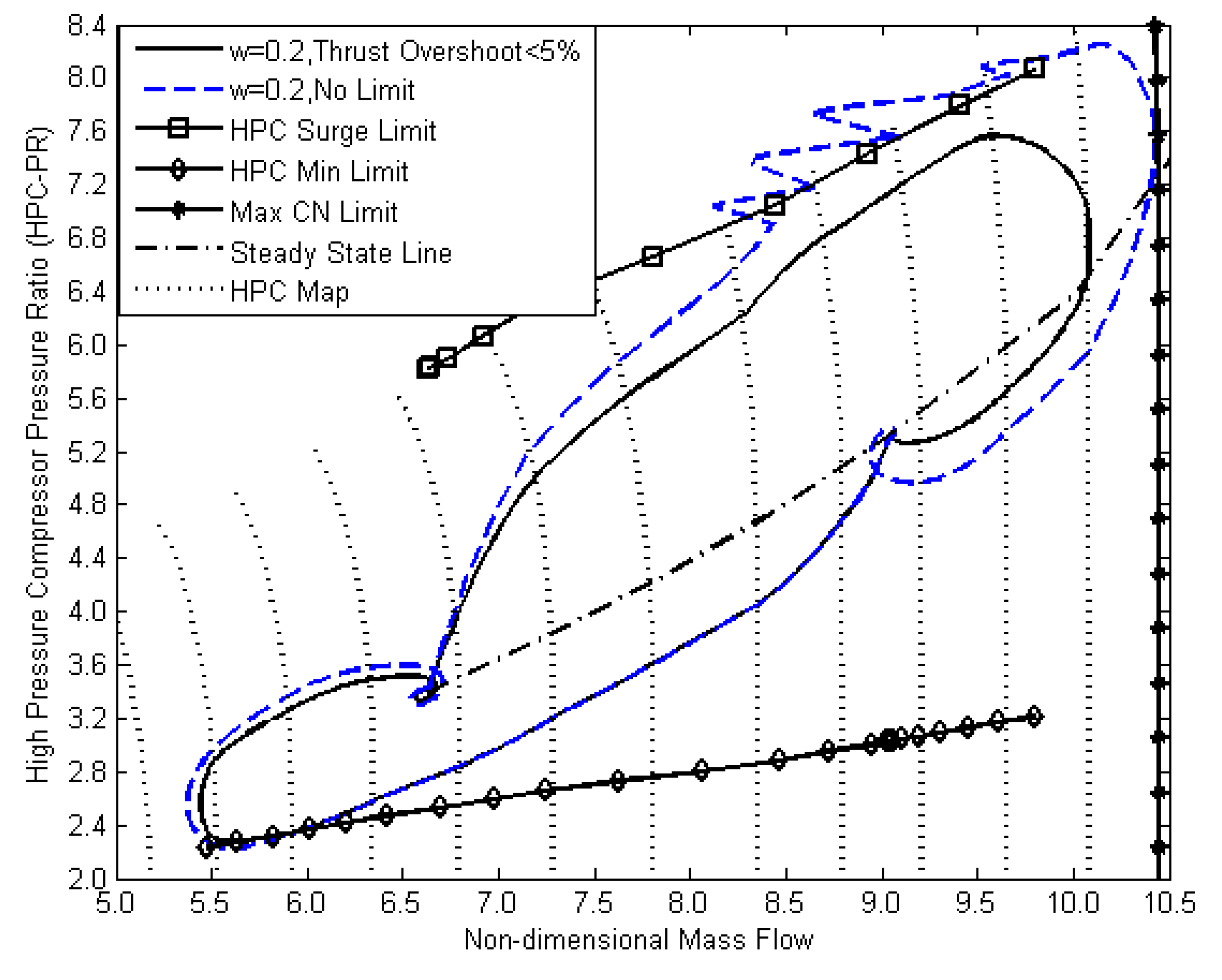
Figure 12 shows the comparison of HPC dynamics with and without the implementation of the surge margin constraint. The penalized transient line includes the constraints shown in Table 2, except for the limits of the HPC-PR, TET, and SFC (Figure 12). The compressor surge exceeding the minimum pressure limit and maximum speed limit occurs when the constraints are removed from the MPC. Preventing compressor surge and combustor flameout requires implementation of the constraints to the HPC-PR. The HPC-PR limits were estimated from the compressor map and implemented as a constraint, which is a linear function of the corrected relative rotational speed of the high-pressure shaft (CNH), as shown in Table 2, so that the limits can evolve together with the variation of the operating points. A rapid transient operation is capable of driving the pressure ratio directly to the boundary lines. As it is demonstrated in Figure 12, the upper limit prevents the compressor from being surged during acceleration. The lower limit prevents engine shutdown due to the lack of compressor exit pressure.
Figure 13 shows the results of transient operations on both compressors, and Figure 14 shows the same operations on the time series. The limit of the gross thrust ratio (Table 2) was designed to maintain the output parameter within the 5% overshoot of the control reference. By removing this limit from the controller, both low and high-pressure shafts were directly driven to their maximum speed limits (Figure 13). The maximum value of the gross thrust ratio (GTR) can reach nearly 130% (30% overshoot) by the acceleration from idle (30%) to 100% of the thrust output, and the maximum speed limits eventually became active on both shafts to stop the further increase of the shaft speed (Figure 14). For a rapid transient operation, the approaching time is normally optimized to 3–5 s, and the percentage of overshoot is required to be controlled to no more than 5% of the target output with a smooth power transition. Therefore, a smaller value of the weighting factor for the MPC (0.2) ensures the satisfaction of the transient time for the entire operating range (Figure 14). As a result, implementing the overshoot limit provides the impact to the shaft speed response, as shown in the solid transient line in Figure 13, retaining a large safety margin to the compressor limits and producing a smoother transient response by reducing the final steady-state oscillations.
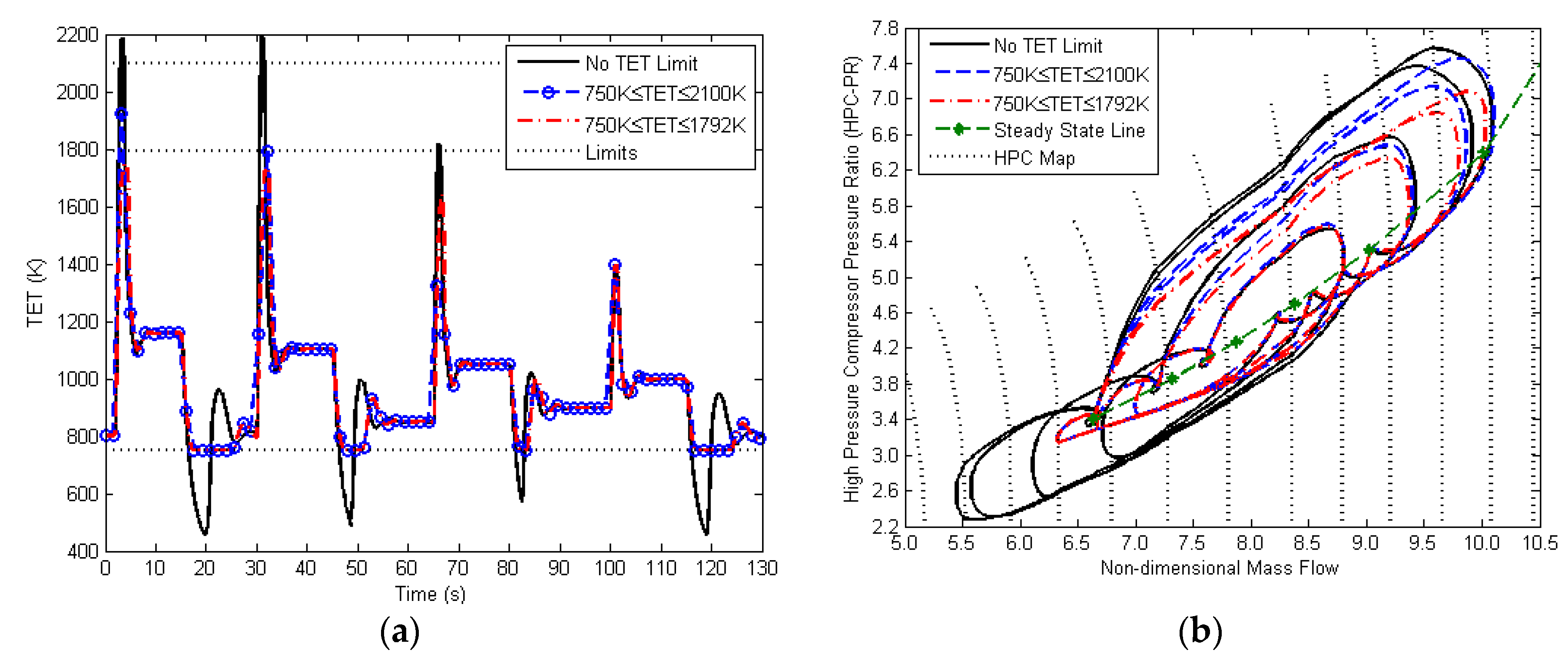
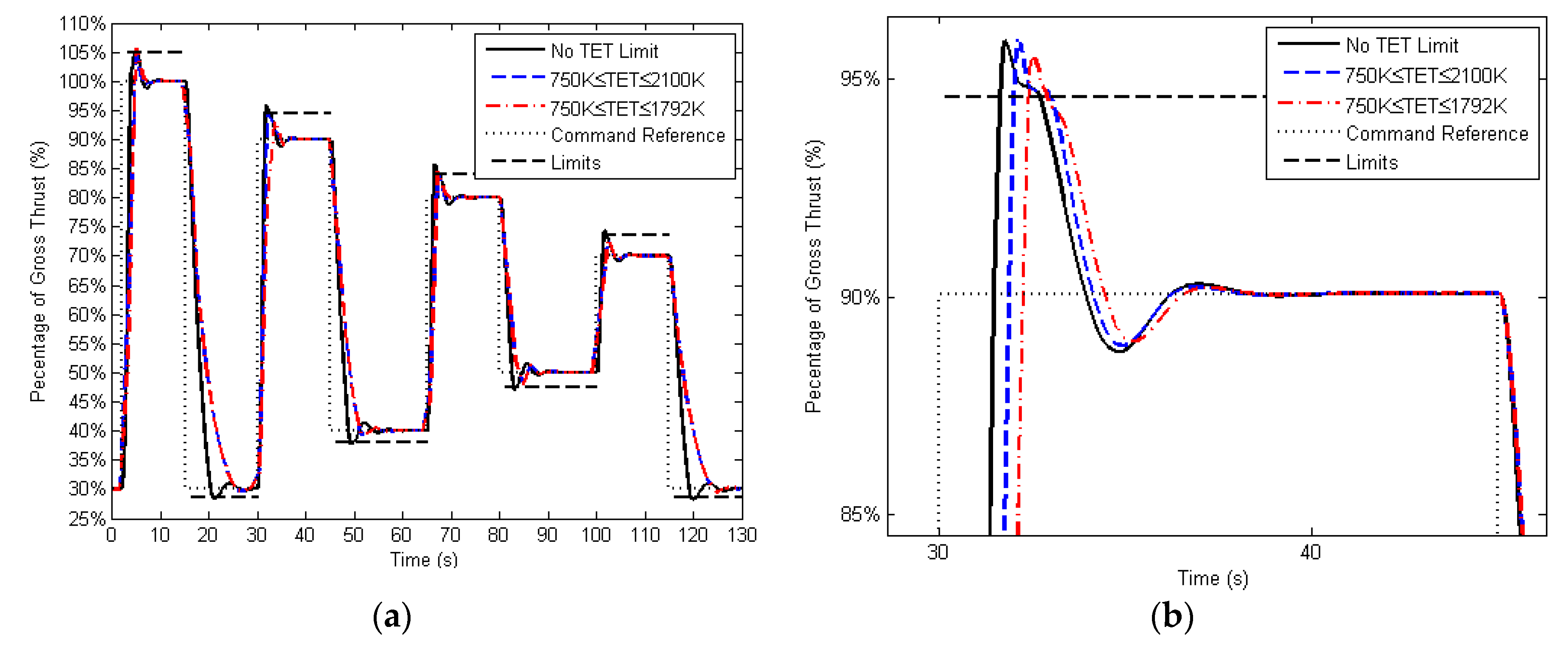
Including the TET limit from Table 2, the MPC monitors the values of TET to prevent the turbine from over-heating. Two different upper limits (1792 K and 2100 K) and one lower limit (679 K) of TET have been included in the test. From Figure 15a, it can be seen that the temperatures can be successfully constrained within their limits throughout the entire operating range. However, longer acceleration and deceleration is produced, as shown in Figure 16. A longer transient time means that a stricter temperature limit has been applied (Figure 16) as well as a larger surge margin, as shown in Figure 15b.
6. Discussion
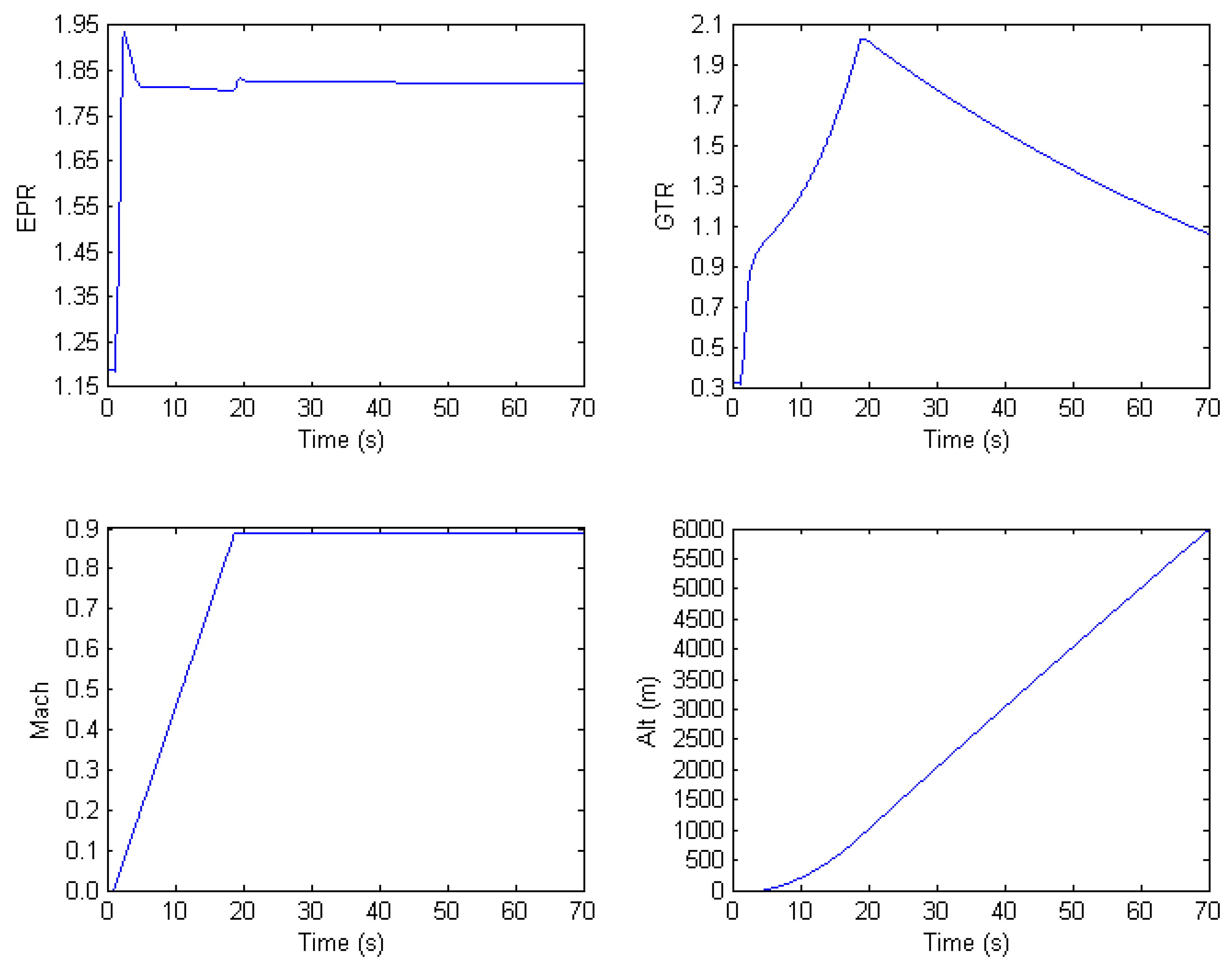
With all the control weights, predictions, and horizon length as well as constraints set-up, the MPC can operate the engine under variable environmental conditions (Figure 17). The MPC accelerated the engine from EPR 1.18 to 1.83 (corresponding from PCNL from 60% to 100% at sea level) within five seconds and maintained the EPR output as close to the final steady-state level as possible while the environmental and the flight condition keeps changing.
In addition to the transient time optimization, fuel economy can be optimized by constraining the maximum fuel flow, the fuel rate, or increasing the control weight to the MPC. However, all of these methods attempt to introduce the actions, which directly influence the input of the fuel value.
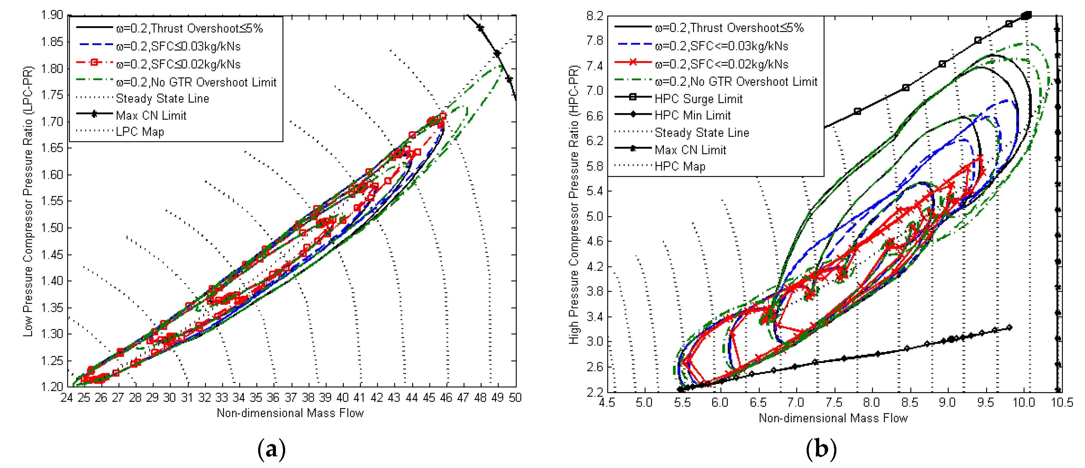
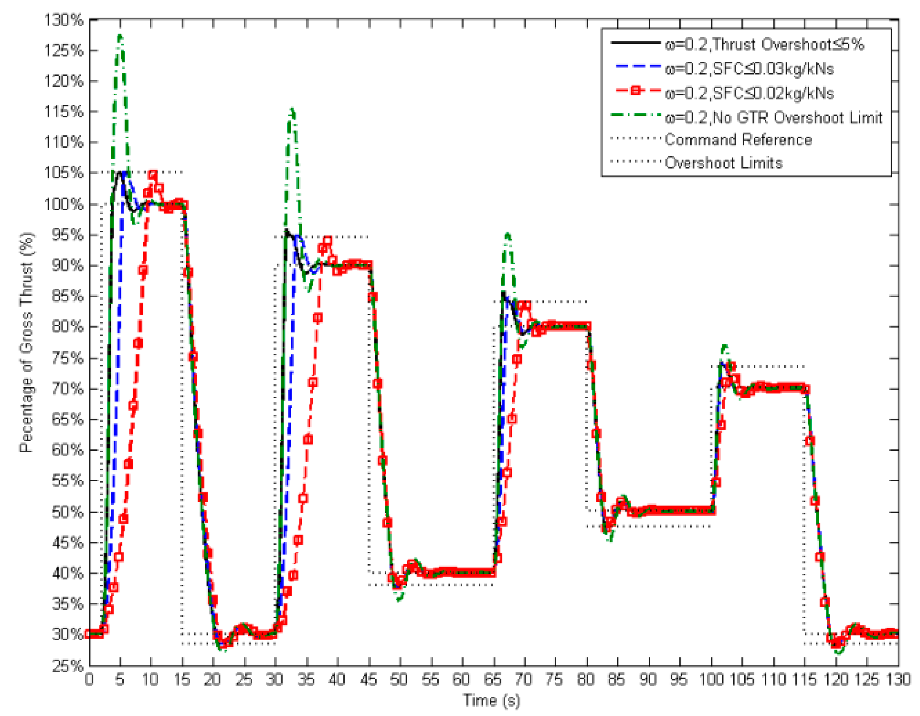
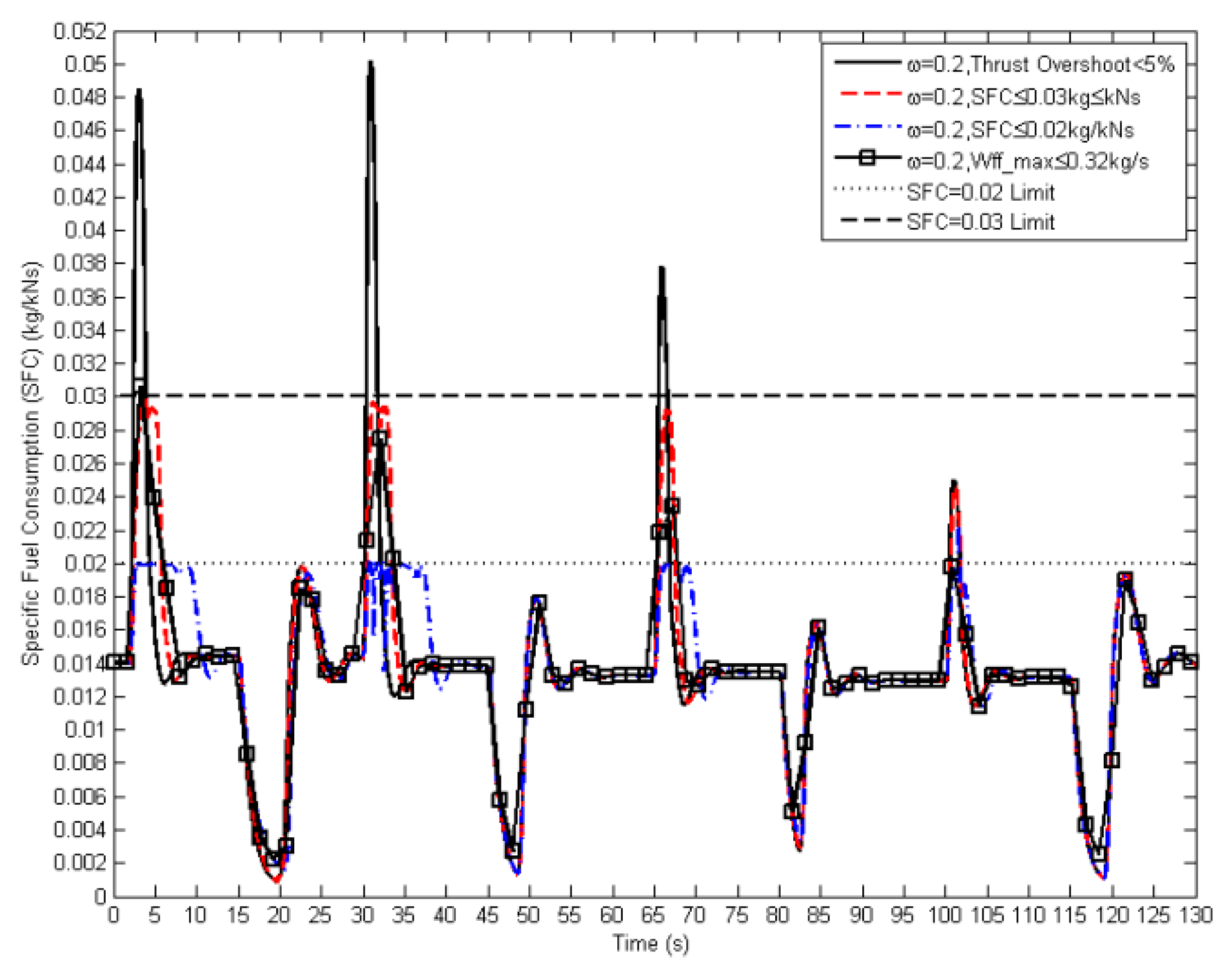
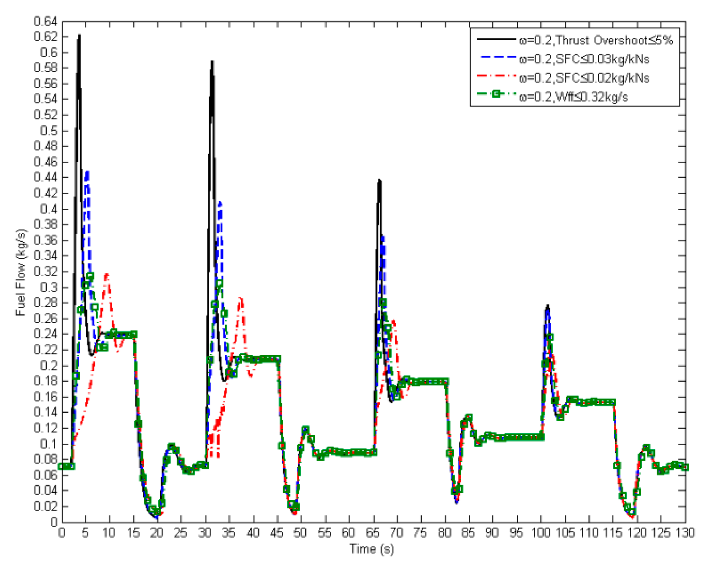
It was found that the value of SFC could be controlled (below 0.03 kg/N∙s) by only limiting the maximum value of fuel flow (Wff ≤ 0.32 kg/s; Figure 18 and Figure 19). Instead, the SFC can be directly added to the constraint, as listed in Table 2. The SFC value was taken as the ratio between the measured fuel flow and the estimated thrust from the engine. The maximum SFC value can be reduced by more than half to the highest peak value given by the transient operation without the limit of SFC. Figure 18 shows that the SFC is successfully kept below the threshold (SFC ≤ 0.03 kg/N∙s and SFC ≤ 0.02 kg/N∙s). The inclusion of an SFC constraint is an example of allowing the controller to monitor engine parameters. By giving a higher control authority to the controller, the more appropriate fuel command can be produced through more specific engine performance restrictions, and different fuel supplies can be determined according to the value given to the engine constraints (Figure 19).
Finally, Table 4 shows the total fuel consumption after the 130 s engine operation test. When the SFC is limited below 0.03 kg/N∙s, the fuel consumption reduces by 2.63%. This value becomes 8.47% when the SFC is limited by a further 0.01 kg/N∙s (SFC ≤ 0.02 kg/Ns). Alternatively, limiting the maximum value of the fuel input means reducing a similar percentage of fuel consumption as well (similar to the results from the constraint of the maximum SFC (0.03 kg/N∙s)).
The total fuel consumption has been increased by 7.57% if a higher value of the weighting factor (ω = 0.8) is used in MPC, due to a longer time in transient states (Table 5). However, if only the first two transient cycles are considered (Figure 19), 0.55% of fuel can be saved by increasing the weighting factor to 0.8.
Consequently, the above results and analyses state that:
The maneuverability of the engine could be achieved by decreasing the weight factor in the designed controller (e.g., 0.2). It will reduce the response time of the engine with the penalty of higher fuel consumption.
The fuel economy will be enhanced by increasing the weighting factor. In this case, the engine response time will be increased as well.
A relatively smaller weighting factor can be applied by the MPC for the parameters, which have a wider cut-off frequency (e.g., GTR and EPR).
In contradictive situations, the designed MPC chooses to satisfy the input limit and compromises the output limit. In other words, the input limits have a higher priority than the output limits.
With a moderate horizon length (70 steps), the controller is capable of allowing the transient operation to be completed within 5 s (≤5% overshoot) as well as saving the computing memory by reducing the columns and rows of constraints in matrix “F”.
Adding more constraints increases the possibility of having less control freedom or a higher chance of contradiction among the constraints. Therefore, it should be taken into account that the definition of a huge number of constraints is not necessarily a positive point in the engine control. The minimum number of required constraints should be defined and formulated.
By utilizing the methodology and results presented in this paper, future studies could be focused on:
- Defining and exploring other constraints, and investigating the effects of ambient temperature and weather conditions.
- Analyzing the fuel consumption for different entry temperatures, and consequently the gas turbine performance.
- Studying the overall vibration of the gas turbine and its effects on the controller and engine performance.
7. Conclusions
A practical constrained model predictive control (MPC) approach is proposed to optimize the real-time transient performance of gas turbine engines for efficient and safe operations. The effectiveness of the algorithm is validated from different points of view by transient simulations of a twin-spool turbofan engine, which is developed by the inter-component volume (ICV) method and validated against Turbomatch, which is an in-house verified gas turbine performance simulation software. Different settings, parameters tuning, and constraints defined for the MPC provide a significant impact on the optimization result of transient performance. However, choosing an appropriate weighting factor value, prediction and control horizons, and implementing a sufficient number of constraints to the engine parameters enables the MPC to control the engine to its best transient performance within the operating and safety requirements.
- The weighting factor is used to adjust the efficiency of the optimization process from the application point of view. A slightly smaller value for the weighting factor ensures that the transient operations can be completed within the specified time for the entire operating range and guarantees the required maneuverability for the engine. However, larger weighting factor values will result in better fuel economy.
- The larger prediction and control length allow the controller to estimate the engine future dynamics with a longer vision. However, the larger the prediction length, the more computational burden to the algorithm. So, a sufficient horizon length should be selected to provide the controller with enough time to plan and realize the control efforts to engine parameters for the satisfaction of the transient time and the performance limitation within the available computing memory.
- Adding constraints to the engine parameters restricts the controller to operate the engine within the operating envelope. The constraints can also be added to improve the performance quality, such as to obtain a fast-transient operation with a limited steady-state overshoot, and to achieve a specific target for fuel consumption (e.g., better fuel economy). However, having more than enough constraints may result in infeasible solutions or huge computational effort.
This research has shown that the constrained MPC can provide the optimal control inputs with no need for the classic scheduling techniques. The MPC is capable of adjusting the fuel flow to adapt the change of the engine performance to the performance requirements and producing the optimal control solution to obtain the optimal transient performance for the entire operating range.
Author Contributions
Conceptualization, T.N. and Z.L.; methodology, T.N. and Z.L.; software, T.N. and Z.L.; validation, Z.L. and S.J.; formal analysis, Z.L. and S.J.; investigation, Z.L.; resources, T.N. and S.J.; writing-original draft preparation, Z.L.; writing-review and editing, T.N. and S.J.; supervision, T.N.
Funding
This research received no external funding.
Conflicts of Interest
The authors declare no conflict of interest.
Nomenclature
| a,b | constant |
| A,B,C,E,F | coefficient matrix |
| CN | corrected relative shaft rotational speed |
| Cp | heat capacity at constant pressure (J/kg∙K) |
| CW | compressor work (N) |
| COT | combustor outlet temperature |
| CMF | constant mass flow |
| ∆H | enthalpy change (J) |
| ∆Q | differential torque (N∙m) |
| DP | design point |
| e | error |
| EPR | engine pressure ratio |
| f | generic functions |
| FAR | fuel–air ratio |
| GTE | gas turbine engine |
| GTR | gross thrust ratio; ratio of gross thrust from engine output to its design point |
| H | enthalpy (J) |
| HP | high-pressure shaft |
| HPC-PR | high-pressure compressor pressure ratio |
| I | moment of inertia for engine model (kg∙m2); identity matrix for MPC |
| ICV | inter-component volume |
| ISA | international standard atmosphere |
| J | objective function |
| k | sampling time, time step |
| LHV | lower heating value (kJ/kg) |
| LP | low pressure shaft |
| LQR | linear–quadratic regulator |
| LPC-PR | low-pressure compressor pressure ratio |
| MIL | matrix inversion lemma |
| MPC | model predictive control |
| m | mass (kg) |
| NDMF | non-dimensional mass flow |
| Np,Nc | prediction, control horizon length |
| NN | neural networks |
| P | pressure for engine model (kPa); covariance matrix for identification process |
| PR | pressure ratio |
| PCNH | percentage of relative rotational speed for high-speed shaft |
| PCNL | percentage of relative rotational speed for low-speed shaft |
| R | gas constant (J/mol∙K) |
| RLS | recursive least squares |
| RLS-SV | recursive least square with varying stabilizing factor |
| SLS | sea level standard |
| SFC | specific fuel consumption |
| T | temperature (K) |
| TET | turbine entry temperature |
| TR | temperature ratio |
| TW | turbine work (N) |
| V | volume (m3) |
| X, U | state, input matrix |
| W | mass flow (kg/s) in engine model; control reference matrix in MPC |
| weighting factor | |
| Wff | engine fuel flow |
| γ | gas constant; constraint matrix for MPC |
| η | efficiency |
| θ | objective parameter |
| φ | parameter matrix |
| µ | forgetting factor |
| Subscripts | |
| L | low-pressure shaft |
| H | high-pressure shaft |
| f | fuel |
References
- Richter, H. Chapter 5 Gain Scheduling and Adaptation. In Advanced Control of Turbofan Engines; Springer: New York, NY, USA, 2011; pp. 91–110. [Google Scholar] [CrossRef]
- Jafari, S.; Montazeri-Gh, M. Evolutionary Optimization for Gain Tuning of Jet Engine Min-Max Fuel Controller. J. Propuls. Power 2011, 27, 1015–1023. [Google Scholar] [CrossRef]
- Kreiner, K.L. The Use of Onboard Real-Time Models for Jet Engine Control; MTU Aero Engines: Munich, Germany, 2002; p. 27. [Google Scholar]
- Jafari, S.; Nikolaidis, T. Turbojet Engine Industrial Min–Max Controller Performance Improvement Using Fuzzy Norms. Electronics 2018, 7, 314. [Google Scholar] [CrossRef] [Green Version]
- Dambrosio, L.; Camporeale, S.; Fortunato, B. Performance of Gas Turbine Power Plants Controlled by One Step Ahead Adaptive Technique; 2000-GT-0037; ASME Turbo Expo: München, Germany, 2000. [Google Scholar]
- Van Essen, H.; Lange, H. Nonlinear Model Predictive Control Experiments on a Laboratory Gas Turbine Installation; 2000-GT-0040; ASME Turbo Expo: München, Germany, 2000. [Google Scholar]
- Orme, J.; Schkolnik, G. Flight Assessment of the Onboard Propulsion System Model for the Performance Seeking Control Algorithm on an F-15 Aircraft; NASA Technical Memorandum 4705; NASA TM-4705; American Institute of Aeronautics and Astronautics, Inc. (AIAA): Reston, VA, USA, 1995. [Google Scholar]
- Directorate-General for Research and Innovation Directorate-General for Mobility and Transport. Flightpath 2050 Europe’s Vision for Aviation Maintaining Global Leadership & Serving Society’s Needs, Report of the High Level Group on Aviation Research; Publications Office of the European Union: Luxembourg, 2011.
- Jafari, S.; Nikolaidis, T. Thermal Management Systems for Civil Aircraft Engines: Review, Challenges and Exploring the Future. Appl. Sci. 2018, 8, 2044. [Google Scholar] [CrossRef] [Green Version]
- Sontag, E. Mathematical Control Theory: Deterministic Finite Dimensional System, 2nd ed.; Springer: Berlin, Germany, 1998; ISBN 0-387-98489-5. [Google Scholar]
- Ali, Q.R.; Mahmoud, S. Application of Optimal control and eigenvalue/eigenvector assignment for Jet engine control. In I Mech E Proceedings C 16/87; Institution of Mechanical Engineers, IMechE: London, UK, 2011; pp. 103–109. [Google Scholar]
- Lutambo, J.; Wang, J. Turbofan Engine Modelling and Control Design using Linear Quadratic Regulator (LQR). Int. J. Eng. Sci. 2017, 6, 49–58. [Google Scholar] [CrossRef]
- Abbott, J. State-Space Control Systems. Utah Telerobotics, University of Utah. Available online: http://www.telerobotics.utah.edu/index.php/StateSpaceControl (accessed on 1 March 2015).
- Samar, R.; Postlethwaite, I. Multivariable Controller Design for a High Performance Aero-Engine. In Proceedings of the 1994 International Conference on Control-Control’94, IET, Coventry, UK, 21–24 March 1994; pp. 1312–1317. [Google Scholar] [CrossRef]
- Kolmanovsky, I.V.; Jaw, L.C.; Merrill, W.; Tran Van, H. Robust Control and Limit Protection in Aircraft Gas Turbine Engines. Control Applications (CCA). In Proceedings of the 2012 IEEE International Conference on Control Applications, Dubrovnik, Croatia, 3–5 October 2012; pp. 812–819. [Google Scholar] [CrossRef]
- Nagahara, M.; Yamamoto, Y.; Miyazaki, S.; Kudoh, T.; Hayashi, N. H∞ Control of Microgrids Involving Gas Turbine Engines and Batteries. In Proceedings of the 51st IEEE Conference on Decision and Control, Maui, HI, USA, 10–13 December 2012. [Google Scholar]
- Esfahani, M.A.; Montazeri-Gh, M. Designing and Optimizing Multi-Objective Turbofan Engine Control Algorithm Using Min-Max Method. Int. J. Comput. Sci. Inf. Secur. 2016, 14, 1040. [Google Scholar]
- Mu, J.; Rees, D. Approximate Model Predictive Control for Gas Turbine Engines. In Proceedings of the 2004 American Control Conference, Boston, MA, USA, 30 June–2 July 2004. [Google Scholar]
- Pandey, A.; de Oliveira, M.; Moroto, R.H. Model Predictive Control for Gas Turbine Engines. In ASME. Turbo Expo: Power for Land, Sea, and Air; Volume 6: Ceramics; Controls, Diagnostics, and Instrumentation; Education; Manufacturing Materials and Metallurgy: Oslo, Norway, 2018; p. V006T05A016. [Google Scholar] [CrossRef]
- Mu, J.; Rees, D. Nonlinear Model Predictive Control for Gas Turbine Engines. In ASME Turbo Expo Power for Land, Sea, and Air; GT2004-53146; ASME: Vienna, Austria, 2004. [Google Scholar]
- Brunell, B.J.; Viassolo, D.E.; Prasanth, R. Model Adaptation and Nonlinear Model Predictive Control of an Aircraft Engine. In ASME Turbo Expo 2004: Power for Land, Sea, and Air; American Society of Mechanical Engineers: New York, NY, USA, 2004; pp. 673–682. [Google Scholar] [CrossRef]
- Brunell, B.J.; Bitmead, R.R.; Connolly, A.J. Nonlinear Model Predictive Control of an Aircraft Gas Turbine Engine. In Proceedings of the 41st IEEE Conference on Decision and Control 2002, Las Vegas, NV, USA, 10–13 December 2002; pp. 4649–4651. [Google Scholar] [CrossRef]
- Aly, A.; Atia, I. Neural Modeling and Predictive Control of a Small Turbojet Engine (SR-30). In Proceedings of the 10th International Energy Conversion Engineering Conference, Atlanta, Georgia, 30 July–1 August 2012; p. 4242. [Google Scholar] [CrossRef]
- Seok, J.; Kolmanovsky, I.; Girard, A. Coordinated Model Predictive Control of Aircraft Gas Turbine Engine and Power System. J. Guid. Control Dyn. 2017, 40, 2538–2555. [Google Scholar] [CrossRef] [Green Version]
- Wang, Y.; Boyd, S. Fast Model Predictive Control Using Online Optimization. IEEE Trans Actions Control Syst. Technol. 2010, 18, 267–278. [Google Scholar] [CrossRef] [Green Version]
- Jafari, S.; Nikolaidis, T. Meta-heuristic global optimization algorithms for aircraft engines modelling and controller design; A review, research challenges, and exploring the future. Prog. Aerosp. Sci. 2019, 104, 40–53. [Google Scholar] [CrossRef]
- Pilidis, P.; Maccallum, N.R.L. A General Program for the Prediction of the Transient Performance of Gas Turbines. In ASME 1985 International Gas Turbine Conference and Exhibit; American Society of Mechanical Engineers: New York, NY, USA, 1985; p. V001T03A053. [Google Scholar] [CrossRef]
- Saravanamuttoo, H.I.H.; Rogers, G.F.C.; Cohen, H. 3. Gas Turbine Cycles for Aircraft Propulsion. In Gas Turbine Theory; Pearson Education: London, UK, 2001. [Google Scholar]
- Rahman, N.U.; Whidborne, J.F. Real-Time Transient Three Spool Turbofan Engine Simulation: A Hybrid Approach. J. Eng. Gas Turbines Power 2009, 131, 051602. [Google Scholar] [CrossRef]
- Kim, S.-K.; Pilidis, P.; Yin, J. Gas Turbine Dynamic Simulation Using Simulink; SAE Technical Paper: Brussels, Belgium, 2000. [Google Scholar] [CrossRef]
- Bücker, D.; Span, R.; Wagner, W. Thermodynamic Property Models for Moist Air and Combustion Gases. J. Eng. Gas Turbines Power 2003, 125, 374–384. [Google Scholar] [CrossRef]
- Nkoi, B.; Pilidis, P.; Nikolaidis, T. Performance assessment of simple and modified cycle turboshaft gas turbines. Propuls. Power Res. 2013, 2, 96–106. [Google Scholar] [CrossRef] [Green Version]
- Torres, M.P.; Sosa, G.; Amezquita-Brooks, L.; Liceaga-Castro, E.; Zambrano-Robledo, P.D.C. Identification of the Fuel-Thrust Dynamics of a Gas Turbo Engine. In Proceedings of the IEEE Conference on Decision and Control, Piscataway, NJ, USA, 10–13 December 2013; pp. 4535–4540. [Google Scholar] [CrossRef]
- Arkov, V.; Evans, C.; Fleming, P.J.; Hill, D.C.; Norton, J.P.; Pratt, I.; Rees, D.; Rodríguez-Vázquez, K. System Identification Strategies Applied to Aircraft Gas Turbine Engines. Annu. Rev. Control 2000, 24, 67–81. [Google Scholar] [CrossRef]
- Paleologu, C.; Benesty, J.; Ciochiňa, S. A Robust Variable Forgetting Factor Recursive Least-Squares Algorithm for System Identification. IEEE Signal Process. Lett. 2008, 15, 597–600. [Google Scholar] [CrossRef]
- Li, Z.; Nikolaidis, T.; Nalianda, D. Recursive least squares for online dynamic identification on gas turbine engines. J. Guid. Control Dyn. 2016, 39, 2594–2601. [Google Scholar] [CrossRef] [Green Version]
- Wang, L. Discrete-Time MPC with Constraints. In Model Predictive Control System Design and Implementation Using MATLAB; Springer: Berlin, Germany, 2009; pp. 2–78. [Google Scholar] [CrossRef]
- Kulikov, G.G.; Thompson, H.A. Dynamic Modelling of Gas Turbines Identification, Simulation, Condition Monitoring and Optimal Control; Springer: London, UK, 2004; ISBN 978-1-4471-3796-2. [Google Scholar] [CrossRef]
- Montazeri-Gh, M.; Jafari, S.; Ilkhani, M.R. Application of particle swarm optimization in gas turbine engine fuel controller gain tuning. Eng. Optim. 2012, 44, 225–240. [Google Scholar] [CrossRef]
- Federal Aviation Administration. Part 33 Airworthiness Standards: Aircraft Engines; U.S. Government Publishing Office: Washington, DC, USA, 2003.
Figure 1.
Schematic of the twin-spool turbofan engine.

Figure 2.
The closed-loop constrained model predictive control (MPC) engine system.

Figure 3.
The natural frequency of LPC-PR (a) and HPC-PR (b) for different levels of power transition and shaft inertias.
Figure 3.
The natural frequency of LPC-PR (a) and HPC-PR (b) for different levels of power transition and shaft inertias.

Figure 4.
The percentage of gross thrust to the design point from the control of MPC with different weighting factors values.
Figure 4.
The percentage of gross thrust to the design point from the control of MPC with different weighting factors values.

Figure 5.
Fuel flow given by MPC with different weighting factor values.

Figure 6.
Close-up percentage gross thrust (a), fuel flow (b).

Figure 7.
The Bode plot of closed loop response of different engine parameters during acceleration (a) and deceleration (b) between 60% and 100% of the percentage of relative rotational speed for a low-speed shaft (PCNL).
Figure 7.
The Bode plot of closed loop response of different engine parameters during acceleration (a) and deceleration (b) between 60% and 100% of the percentage of relative rotational speed for a low-speed shaft (PCNL).

Figure 8.
Transient operation between 60% and 100% of PCNL using gross thrust ratio (GTR), engine pressure ratio (EPR) and PCNL as the control reference.
Figure 8.
Transient operation between 60% and 100% of PCNL using gross thrust ratio (GTR), engine pressure ratio (EPR) and PCNL as the control reference.

Figure 9.
The Bode plot of closed loop response of EPR during acceleration (a) and deceleration (b) of different transient ranges between 60% and 100% of PCNL.
Figure 9.
The Bode plot of closed loop response of EPR during acceleration (a) and deceleration (b) of different transient ranges between 60% and 100% of PCNL.

Figure 10.
Comparison of transient acceleration for different operation ranges controlled by MPC and PID.
Figure 10.
Comparison of transient acceleration for different operation ranges controlled by MPC and PID.

Figure 11.
Percent total gross thrust to the design point given by MPC with different prediction length.
Figure 11.
Percent total gross thrust to the design point given by MPC with different prediction length.

Figure 12.
The comparison of HPC transient performance with and without limits of engine parameters.
Figure 12.
The comparison of HPC transient performance with and without limits of engine parameters.

Figure 13.
LPC (a) and HPC (b) transient performance controlled by MPC with different definitions of parameter constraints.
Figure 13.
LPC (a) and HPC (b) transient performance controlled by MPC with different definitions of parameter constraints.

Figure 14.
The gross thrust under the control of MPC with different definitions of parameter constraints.
Figure 14.
The gross thrust under the control of MPC with different definitions of parameter constraints.

Figure 15.
The performance of turbine entry temperature (TET) (a) and the HPC (b) affected by the limited TET compared to the results from the control of MPC without TET constraint.
Figure 15.
The performance of turbine entry temperature (TET) (a) and the HPC (b) affected by the limited TET compared to the results from the control of MPC without TET constraint.

Figure 16.
(a) The transient performance of output gross thrust ratio (GTR) with the limitation of TET; (b) the close-up view.
Figure 16.
(a) The transient performance of output gross thrust ratio (GTR) with the limitation of TET; (b) the close-up view.

Figure 17.
Transient acceleration under increase of Mach number and altitude.

Figure 18.
SFC from transient performance controlled by MPC with different definitions of constraint settings.
Figure 18.
SFC from transient performance controlled by MPC with different definitions of constraint settings.

Figure 19.
Comparison of fuel flow given by MPC with constraints.


Table 1.
Design point of the twin-spool turbofan engine.
| Ambient condition | ISA SLS | [-] |
| Intake Mach number | 0 | [-] |
| Intake mass flow | 44.8 | kg/s |
| Low-pressure compressor pressure ratio (LPC-PR) | 1.70 | [-] |
| Low-pressure compressor isentropic efficiency | 88 | % |
| High-pressure compressor pressure ratio (HPC-PR) | 5.60 | [-] |
| High-pressure compressor isentropic efficiency | 88 | % |
| Bypass ratio | 0.69 | [-] |
| Fuel flow | 0.2466 | kg/s |
| High-pressure turbine isentropic efficiency | 89 | % |
| Low-pressure turbine isentropic efficiency | 89 | % |
| Moment of inertia for low-pressure shaft | 10 | Nm2 |
| Moment of inertia for high-pressure shaft | 8.4 | Nm2 |
| Percentage of low-pressure shaft corrected rotational speed at 170 RPS | 100 | % |
| Percentage of high-pressure shaft corrected rotational speed at 177 RPS | 100 | % |
| Volume 1 | 1.50 | m3 |
| Volume 2 | 0.50 | m3 |
| Volume 3 | 0.38 | m3 |
| Volume 4 | 0.50 | m3 |
Table 2.
Numerical procedure and solution for the modeling, control, and constraints definition procedures.
Table 2.
Numerical procedure and solution for the modeling, control, and constraints definition procedures.
| 1 | Step 1: Modeling Phase | Mathematical model generation and updates | Equations (1)–(6) |
| 2 | Step 2: Control Phase | MPC design and tuning | Equations (7)–(15) |
| 3 | Step 3: Constraints Definition Phase | Constraints definition | Equations (16)–(19) |
| 4 | Step 4: Solution Phase | Optimal control solution definition | Equations (20)–(21) |
Table 3.
The constraints to the engine parameters.
| 0.002 kg/s ≤ Wff ≤ 1.20 kg/s |
| −0.80 kg/s ≤ ΔWff ≤ 0.80 kg/s |
| 55% ≤ CNL ≤ 105% |
| 71% ≤ CNH ≤ 112% |
| PRHPC|surge = f(CNH) = 9.5625∙CNH − 2.1096 |
| PRHPC|idle = f(CNH) = 3.0198∙CNH + 0.0180 |
| 680K ≤ TET ≤ 2100K or 1792K |
| −5% ≤ GTRovershoot or EPR or CNL ≤ 5% |
| SFC ≤ 0.03 or 0.02 kg/kN∙s |
Table 4.
Gain schedule.
| Operation Range of PCNL | Proportional Gain (P) | Integral Gain (I) |
|---|---|---|
| 60–70% | 0.4 | 0.6 |
| 70–80% | 0.4 | 0.5 |
| 80–90% | 0.3 | 0.4 |
| 90–100% | 0.2 | 0.3 |
Table 5.
Total fuel consumption (kg) for 130 s simulation.
| ω = 0.2 | 18.04 |
| ω = 0.8 | 19.40 (+7.57%) |
| ω = 0.2, no overshoot limit | 18.40 (+1.99%) |
| ω = 0.2, Wff ≤ 0.32 kg/s | 17.50 (−2.99%) |
| ω = 0.2, SFC ≤ 0.03 kg/Ns | 17.56 (−2.63%) |
| ω = 0.2, SFC ≤ 0.02 kg/Ns | 16.51 (−8.47%) |
© 2019 by the authors. Licensee MDPI, Basel, Switzerland. This article is an open access article distributed under the terms and conditions of the Creative Commons Attribution (CC BY) license (http://creativecommons.org/licenses/by/4.0/).
Share and Cite
MDPI and ACS Style
Nikolaidis, T.; Li, Z.; Jafari, S. Advanced Constraints Management Strategy for Real-Time Optimization of Gas Turbine Engine Transient Performance. Appl. Sci. 2019, 9, 5333. https://0-doi-org.brum.beds.ac.uk/10.3390/app9245333
AMA Style
Nikolaidis T, Li Z, Jafari S. Advanced Constraints Management Strategy for Real-Time Optimization of Gas Turbine Engine Transient Performance. Applied Sciences. 2019; 9(24):5333. https://0-doi-org.brum.beds.ac.uk/10.3390/app9245333
Chicago/Turabian StyleNikolaidis, Theoklis, Zhuo Li, and Soheil Jafari. 2019. "Advanced Constraints Management Strategy for Real-Time Optimization of Gas Turbine Engine Transient Performance" Applied Sciences 9, no. 24: 5333. https://0-doi-org.brum.beds.ac.uk/10.3390/app9245333
Note that from the first issue of 2016, this journal uses article numbers instead of page numbers. See further details here.