
Decompositions of the λ-Fold Complete Mixed Graph into Mixed 6-Stars
1
Department of Mathematics and Statistics, East Tennessee State University, Johnson City, TN 37614, USA
2
Industrial & Systems Engineering, University of Tennessee, Knoxville, TN 37996, USA
*
Author to whom correspondence should be addressed.
†
These authors contributed equally to this work.
AppliedMath 2024, 4(1), 211-224; https://0-doi-org.brum.beds.ac.uk/10.3390/appliedmath4010011
Submission received: 22 November 2023
/
Revised: 15 January 2024
/
Accepted: 24 January 2024
/
Published: 5 February 2024
Abstract
:Graph and digraph decompositions are a fundamental part of design theory. Probably the best known decompositions are related to decomposing the complete graph into 3-cycles (which correspond to Steiner triple systems), and decomposing the complete digraph into orientations of a 3-cycle (the two possible orientations of a 3-cycle correspond to directed triple systems and Mendelsohn triple systems). Decompositions of the -fold complete graph and the -fold complete digraph have been explored, giving generalizations of decompositions of complete simple graphs and digraphs. Decompositions of the complete mixed graph (which contains an edge and two distinct arcs between every two vertices) have also been explored in recent years. Since the complete mixed graph has twice as many arcs as edges, an isomorphic decomposition of a complete mixed graph into copies of a sub-mixed graph must involve a sub-mixed graph with twice as many arcs as edges. A partial orientation of a 6-star with two edges and four arcs is an example of such a mixed graph; there are five such mixed stars. In this paper, we give necessary and sufficient conditions for a decomposition of the -fold complete mixed graph into each of these five mixed stars for all .
1. Introduction
1.1. Outline
In this paper, we give necessary and sufficient conditions for the existence of mixed 6-star decompositions of the -fold complete mixed graph. In Section 1.2, we give well-known definitions of graph and digraph. Based on the form of these definitions, we define the less well-known objects of fuzzy graph and mixed graph. A broad description of applications of these is mentioned. The main result of this paper concerns a mixed graph decomposition, so in Section 1.3 we define decompositions of graphs/multigraphs, digraphs/multidigraphs, and mixed graphs/multi-mixed graphs, and relate these concepts to each other. Section 2 is the main body of the paper and includes a description of the proof technique, background results, and a statement and proof of the main result. In Section 2.1, we explain the primary proof technique (“difference methods”) used in a large part of the construction, which establishes the validity of our main result. In Section 2.2, we elaborate on the construction method and described a modified difference method that is also employed in our construction. Section 2.3 includes a background result and a lemma containing necessary conditions for the decomposition of interest. In Section 2.4, we give several theorems that combine to give necessary and sufficient conditions for our main result, namely a decomposition of the -fold complete mixed graph into mixed 6-stars. Section 3 discusses the applications of graph decompositions in general, the application of the proof technique to other possible mixed graph structures, and suggests some future directions for additional research.
1.2. Graph Definitions
We largely follow the graph theoretic definitions set out in [1]. A (simple) graph is a pair of (finite) sets , where the elements of are 2-element subsets of . The elements of V are called vertices (though the term nodes is also common) and the elements of E are called edges. Edge is said to join vertices u and v; we will often denote edge as . The complete graph on v vertices, denoted , is the graph with vertex set V, where and . A cycle of length v, denoted , is the graph with vertex set and edge set . A star on vertices, denoted , is a graph with vertex set and edge set . A multigraph is a pair where (finite) set V is the vertex set and E is a (finite) multiset (that is, a finite collection that allows elements to appear a repeated number of times), where the elements of E are multisets of two, not necessarily distinct, elements of V. An element of E of the form is a loop on v. The -fold complete graph on v vertices, denoted , is the multigraph with vertex set V, where and E contains every edge , where , exactly times.
Applications have been part of the reason for the pursuit of graph theory since its origins. One of the most famous graph theory problems (likely due to its difficulty and wide-ranging applications) is the traveling salesman problem. Introduced to find a minimal weighted spanning tree in a given weighted graph, applications of the problem appear in genome mapping, aiming telescopes, guiding machines through a sequence of tasks, and organizing data. In addition, the difficulty of the problem has had an impact on the study of computational complexity and the study of algorithms; for details on this, see [2]. The “assignment problem” (also called the “scheduling problem”) involves finding a maximal matching in a bipartite graph and can be applied to matching a group of workers, each with a certain set of skills, with a group of jobs, each of which requires a certain set of skills [3] (see Section 7.2), ref. [4] (see Section 16.1 and Problem 16.2). The areas of application of graph theory are growing rapidly in the 21st century. In particular, graph neural networks (or “deep learning on graphs”) have received remarkable levels of attention. Applications include computer vision, language recognition, automated planning, social networks, bioinformatics, and cybersecurity [5] (page vii).
A (simple) digraph (or directed graph) is a pair of (finite) sets, , together with two maps, and . Again, the elements of V are called vertices. The elements of A are called arcs (or directed edges). For arc , we call the initial vertex of a and the terminal vertex of a, and we denote a as the ordered pair . The complete digraph on v vertices, denoted , is the graph with vertex set V, where and . A multidigraph is a pair, , where (finite) set V is the vertex set and A is a (finite) multiset, where the elements of A are arcs of the form , where . The -fold complete digraph on v vertices, denoted , is the multidigraph with vertex set V, where and A contains every arc , where , exactly times. A digraph (or multidigraph), D, is an orientation of an (undirected) graph (or multigraph), G, if , and for each we have either or (but not both, unless this results from multiple appearances of edge in ).
A mixed graph is a triple of finite sets , where V is a set of vertices, E is a set of edges (as defined above for graph ), and A is a set of arcs (as defined above for digraph ). A multi-mixed graph is a triple , where V is a set of vertices, E is a multiset of edges (as defined above for multigraph ), and A is a multiset of arcs (as defined above for multidigraph ). We note that Harary and Palmer, who first introduced mixed graphs in 1966, defined a mixed graph as containing “both ordinary and oriented lines” [6]. They followed a convention of combining two anti-parallel arcs into a single edge. We deviate from this practice in our definition and allow the presence of both an edge and two anti-parallel arcs between a pair of vertices (as has become more common in recent years). The complete mixed graph on v vertices, denoted , is the mixed graph , where , edge set E contains each edge , where , exactly once, and arc set A contains every arc , where , exactly once. The -fold complete multi-mixed graph on v vertices, denoted , is the multi-mixed graph with vertex set V, where , multiset E contains every edge , where , exactly times, and multiset A contains every arc , where , exactly times. A multi-mixed graph, M, is a partial orientation of an (undirected) graph (or multigraph), G, if , , and for every edge we have either or (but not both, unless this results from multiple appearances of edge in ).
Of additional interest is the idea of a fuzzy graph. An outgrowth of fuzzy logic (which has recently found a huge number of applications, particularly in the areas of machine learning and artificial intelligence), the theory of fuzzy graphs involves structures that do not fall into the binary relationships of “element of” and “not an element of”, but instead involves a degree of membership (which can be interpreted as a probability of membership). We rely on [7] for definitions and descriptions of this topic, though we modify the notation slightly for consistency with our other definitions. For a given set, X, a fuzzy subset of X (or simply a “fuzzy set”) is a function, , mapping . A fuzzy graph is a quadruple , where V is a finite set of vertices, E is a set of edges (as defined above for graph ), and and are functions, where and , which satisfy the condition for all . Fuzzy set is the fuzzy vertex set of F and fuzzy set is the fuzzy edge set of F. Applications of fuzzy graph theory include cluster analysis and decision analysis in statistical science, pattern classification, neural networks, and social science [7] (page 1). Recent examples of applications of fuzzy graph theory include the use of the concept of the “Randic index” in a connected system applied to Indonesian tourism [8], and the use of Cartesian products, compositions, and unions of “picture fuzzy graphs” applied to railway networks and medical science models [9].
1.3. Decomposition Definitions
A g-decomposition of graph G is a set of subgraphs of G, , where for , for , and . The are called blocks of the decomposition. When G is a complete graph, the g-decomposition is often called a graph design. A -decomposition of is a Steiner triple system of order v, and it is well known that such a triple system exists if and only if or 3 (mod 6) (see [10] for references). Cycle graph designs were a topic of intense interest until the early 2000s, when necessary and sufficient conditions for a -decomposition of were given for all m and v [11,12]. An easier and self-contained construction for odd cycle systems is given in [13]. Necessary and sufficient conditions for decompositions of into copies of (not necessarily isomorphic) stars are given in [14]. To illustrate the potential application of graph decompositions, consider a (hypothetical) machine that runs samples three at a time. The machine can only make comparisons between samples that are run together in the machine (it cannot be calibrated from run to run, say). If one desires to compare a collection of samples of size v, can this be done optimally (that is, by comparing every pair of samples exactly once)? By representing the samples as vertices of a graph, comparisons of a pair of samples as an edge, and a run of the machine as a , an optimal solution is equivalent to a Steiner triple system of order v, and the subgraphs in the decomposition give the runs of the machine in the optimal solution. A g-decomposition of multigraph G is defined similar to that of a g-decomposition of a graph, with the edges of G repeated an appropriate number of times in the multiset of the . Necessary and sufficient conditions for a -decomposition of are given in [15]. Notice that the three-at-a-time comparison application can be solved, if exactly comparisons per pair of samples is required, by considering a -decomposition of .
A d-decomposition of digraph D is a set of subdigraphs of D, , where for , for , and . The are called blocks of the decomposition. When D is a complete digraph, the d-decomposition is often called a digraph design. There are two orientations of , a 3-circuit (in which case the three arcs are oriented in the “same” direction, say clockwise) and the transitive triple (say, with two clockwise-oriented arcs and one counterclockwise-oriented arc). A decomposition of into 3-circuits is a Mendelsohn triple system of order v, and a decomposition of into transitive triples is a directed triple system of order v. Each of these exists if and only if or 1 (mod 3), , except in the case of for a Mendelsohn triple system [16,17]. A d-decomposition of multidigraph D is defined similar to that of a d-decomposition of a digraph, with the arcs of D repeated an appropriate number of times in the multiset of the . Decompositions of into Mendelsohn triples are considered in [18] and decompositions of into transitive triples are considered in [19]. The literature on graph designs and graph decompositions (and of digraph decompositions) is extensive [10,20], especially in the case of triple systems [21].
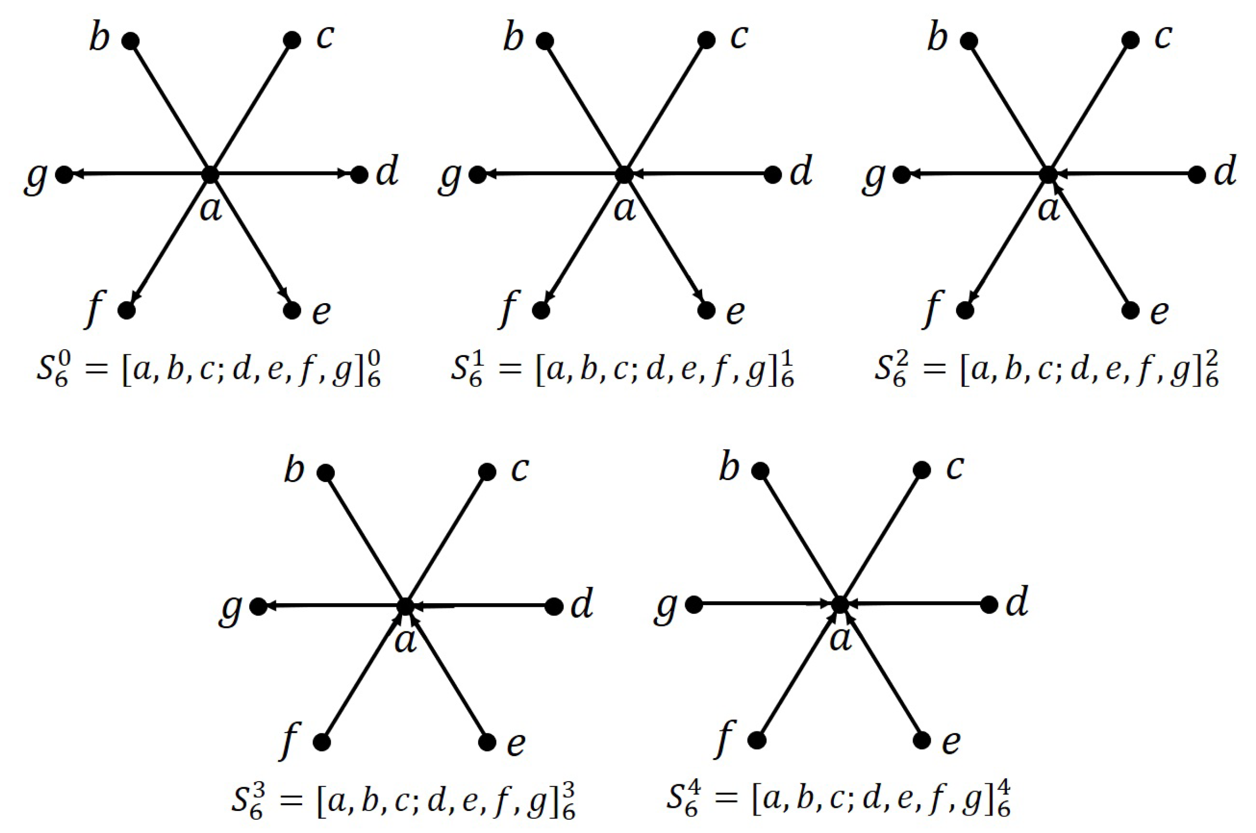
An m-decomposition of mixed graph M is a set of sub-mixed graphs of M, , where for , and for , , and . The are called blocks of the decomposition. When M is a complete mixed graph, the m-decomposition is often called a mixed graph design. Since the complete mixed graph, , has twice as many arcs as edges, then for an m-decomposition of we must have that m also has twice as many arcs as edges. This gives a necessary condition for the existence of a mixed graph design. For example, each partial orientation of with two arcs and one edge could yield a decomposition of . Such a decomposition is called a mixed triple system of order v. Necessary and sufficient conditions for the existence of the various types of mixed triple systems of order v are given in [22]. A partial orientation of the star with two arcs and one edge could yield a decomposition of . Necessary and sufficient conditions for the existence of a decomposition of is given for each such partial orientation of in [23]. Of particular interest to the current work is the decomposition of into partial orientations of with four arcs and two edges; such mixed graph designs are classified in [24]. An m-decomposition of multi-mixed graph M is defined similar to that of an m-decomposition of a mixed graph, with the arcs of M repeated an appropriate number of times in the multiset of the . The purpose of this paper is to classify decompositions of into partial orientations of with four arcs and two edges for all . In this way, the research gap between decompositions of simple mixed graphs and decompositions of multi-mixed graphs is filled in the case of partial orientations of . There are five partial orientations of with four arcs and two edges, and these are given in Figure 1.
2. Decompositions of the -Fold Complete Mixed Graph into Mixed 6-Stars
2.1. Difference Methods
For the complete mixed graph , we take . Define the edge difference associated with edge as . Define the arc difference associated with arc as . Notice that the total set of edge differences associated with E is , and the total set of arc differences associated with A is . Under the permutation , the orbit of the edge includes all edges of , with associated edge difference . Similarly, under permutation , the orbit of arc includes all arcs of , with associated arc differences . Suppose , where for , is a collection of sub-mixed graphs of , such that every edge difference (respectively, arc difference ) is associated with exactly one edge (respectively, arc) in the edge sets (respectively, arc sets) of the . Then, if we take all of the images of the under the powers of , we obtain an m-decomposition of , with . The set is a set of base blocks for the m-decomposition of under . Similarly, if multiset contains edges and arcs that give each edge difference and each arc difference exactly times, then the images of the under the powers of give an m-decomposition of . This is the construction technique often used in the proof of the main result of this paper when v is odd.
2.2. Automorphisms of Decompositions
An automorphism of a decomposition, , of graph is a permutation of V that fixes set . Automorphisms of a digraph decomposition and of a mixed graph decomposition (as well as the multigraph/multidigraph/multi-mixed graph versions) are similarly defined. A decomposition admitting the automorphism of Section 2.1 is a cyclic decomposition. Cyclic automorphisms and difference methods are a frequently used method of construction for various decompositions. For example, a cyclic Steiner triple system of order v exists for all possible orders or 3 (mod 6), except for . The construction of such systems, along with an explanation of the difference methods used, is given in [10].
A decomposition of one of the classes of graphs discussed, where , which admits the automorphism , is a rotational decomposition. Rotational Steiner triple systems were the first class of objects studied in terms of the question: “For what orders does a graph decomposition admit a given type of permutation as an automorphism?” [25]. The use of a rotational permutation in the construction of a decomposition is related to the idea of difference methods, as discussed in Section 2.1. However, the differences are associated with the cycle of length , and edges and/or arcs to/from the fixed point ∞ must be taken into consideration. When using a rotational permutation, a set of base blocks would need each edge/arc difference to be present an appropriate number of times (either 1 or ), and an edge/arc with ∞ as an end/terminal end/initial end would need to be present an appropriate number of times (either 1 or each). We often use rotational permutations in the proof of the main result of this paper when v is even.
2.3. Background Result and a Lemma
The necessary and sufficient conditions for the existence of an -decomposition of are as follows [24].
Theorem 1.
An -decomposition of exists if and only if ,
- 1.
- if then (mod , and
- 2.
- if then or 1 (mod .
The next lemma gives necessary conditions for the existence of an -decomposition, where , of when is odd.
Lemma 1.
For λ odd and , if an -decomposition of exists then or 1 (mod .
Proof.
First, notice that for odd and (mod 4), say , the number of edges of is , which is odd. In this case, no -decomposition of exists since has two edges.
Next, for odd and (mod 4), say , the number of edges of is , which is odd. In this case, no -decomposition of exists.
Therefore, if an -decomposition of exists then or 1 (mod , as claimed. □
2.4. The Decomposition Theorem and Proof
Since has seven vertices for each i, then of course a necessary condition for an -decomposition of any mixed graph on v vertices is . In several of the following constructions, we take as the vertex set of . We will also use the permutation in several of the constructions. We now give necessary and sufficient conditions for the existence of an -decomposition of in each case (with the exception of the small cases and when and , which we leave open).
Theorem 2.
An -decomposition of exists if and only if and
- 1.
- (mod and (mod , or
- 2.
- (mod and , or
- 3.
- (mod and (mod .
Proof.
Each vertex of has out-degree and each vertex of has out-degree 0 (mod 4) so, if an -decomposition of exists, then (mod 4) is necessary. This observation, along with Lemma 1, gives the necessary conditions. We now show these necessary conditions are sufficient.
Case 1. Suppose (mod 4), , say where , and (mod 4). Consider the blocks:
These blocks, along with their images under powers of permutation , form an -decomposition of . By taking copies of the blocks of such a decomposition, we obtain an -decomposition of .
Case 2. Suppose (mod 4). Then by Theorem 1 an -decomposition of exists by Theorem 1. For any , we take copies of the blocks of such a decomposition and this gives an -decomposition of .
Case 3. Suppose (mod 4), , say where , and (mod 4). Consider the blocks
These blocks, along with their images under powers of permutation , form an -decomposition of . By taking copies of the blocks of such a decomposition, we obtain an -decomposition of .
Case 4a. Suppose . Consider the blocks
These blocks, along with their images under powers of permutation , form an -decomposition of . By taking copies of the blocks of such a decomposition, we obtain an -decomposition of .
Case 4b. Suppose (mod 4), , say where , and (mod 4). Consider the blocks
These blocks, along with their images under powers of permutation , form an -decomposition of . By taking copies of the blocks of such a decomposition, we obtain an -decomposition of . □
Since is self-converse and the converse of is , then an -decomposition of exists if and only if an -decomposition of exists. So, the conditions for the existence of an -decomposition of , given in Theorem 2, are also the conditions for the existence of an -decomposition of .
Theorem 3.
An -decomposition of exists if and only if and
- 1.
- or 1 (mod and , where when , or
- 2.
- (mod and (mod , or
- 3.
- (mod and (mod ,
with the possible exceptions of and when , which we leave open.
Proof.
Theorem 1 and Lemma 1 give the necessary conditions. We now show these necessary conditions are sufficient.
Case 1a. Suppose . Consider the blocks
These blocks, along with their images under powers of permutation , form an -decomposition of . Consider the blocks
These blocks, along with their images under powers of permutation , form an -decomposition of . Consider the blocks
These blocks, along with their images under powers of permutation , form an -decomposition of . Since any can be written as a sum of a multiple of 3 and a multiple of 4 (except for 5), then an -decomposition of , where , exists and can be constructed by taking appropriate numbers of copies of decompositions of and (with the exception of , which we have dealt with separately).
Case 1b. Suppose or 1 (mod 4), . Then by Theorem 1 an -decomposition of exists by Theorem 1. For any , we take copies of the blocks of such a decomposition and this gives an -decomposition of .
Case 2a. Suppose . Consider the blocks
These blocks, along with their images under powers of permutation , form an -decomposition of . Consider the blocks
These blocks, along with their images under powers of permutation , form an -decomposition of . Since any even can be written as a sum of a multiple of 4 and a multiple of 6, then an -decomposition of , where is even, exists and can be constructed by taking appropriate numbers of copies of decompositions of and .
Case 2b. Suppose . Consider the blocks
These blocks, along with their images under powers of permutation , form an -decomposition of . By taking copies of the blocks of such a decomposition, we obtain an -decomposition of .
Case 2c. Suppose (mod 8), say where , and (mod 2). Consider the blocks
These blocks, along with their images under powers of permutation , form an -decomposition of . By taking copies of the blocks of such a decomposition, we obtain an -decomposition of .
Case 3. Suppose (mod 4), , say where , and (mod 2). Consider the blocks
These blocks, along with their images under powers of permutation , form an -decomposition of . By taking copies of the blocks of such a decomposition, we obtain an -decomposition of .
Case 4. Suppose (mod 8), , say where , and (mod 2). Consider the blocks
These blocks, along with their images under the powers of permutation , form an -decomposition of . By taking copies of the blocks of such a decomposition, we obtain an -decomposition of . □
Since is self-converse and the converse of is , then an -decomposition of exists if and only if an -decomposition of exists. So, the conditions for the existence of an -decomposition of , given in Theorem 3, are also the conditions for the existence of an -decomposition of (with the exceptions of and when ).
Theorem 4.
An -decomposition of exists if and only if and
- 1.
- or 1 (mod and , where in the case , or
- 2.
- (mod and (mod , or
- 3.
- (mod and (mod .
Proof.
Theorem 1 and Lemma 1 give the necessary conditions. We now show these necessary conditions are sufficient.
Case 1a. Suppose or 1 (mod 4), . Then by Theorem 1 an -decomposition of exists by Theorem 1. For any , we take copies of the blocks of such a decomposition and this gives an -decomposition of .
Case 1b. Suppose . Take the blocks of an -decomposition of (which exists by Case 1a), where the vertices of are . To this, add the images of under the permutation . This gives an -decomposition of , where the vertex set is . Next, consider the blocks:
These blocks, along with their images under permutation , form an -decomposition of . Since any can be written as a sum of a multiple of 2 and a multiple of 3, then an -decomposition of , where , exists and can be constructed by taking appropriate numbers of copies of decompositions of and .
Case 2a. Suppose . Take the blocks of an -decomposition of (which exists by Case 1a), where the vertices of are . To this, add the images of under the permutation . This gives an -decomposition of , where the vertex set is . By taking copies of the blocks of such a decomposition, we obtain an -decomposition of for all even .
Case 2b. Suppose . Consider the blocks
These blocks, along with their images under permutation , form an -decomposition of . By taking copies of the blocks of such a decomposition, we obtain an -decomposition of for all even .
Case 2c. Suppose (mod 8), say where , and (mod 2). Consider the blocks
These blocks, along with their images under the powers of permutation , form an -decomposition of . By taking copies of the blocks of such a decomposition, we obtain an -decomposition of .
Case 3. Suppose (mod 4), , say where , and (mod 2). Consider the blocks
These blocks, along with their images under powers of permutation , form an -decomposition of . By taking copies of the blocks of such a decomposition, we obtain an -decomposition of .
Case 4. Suppose (mod 8), , say where , and (mod 2). Consider the blocks
These blocks, along with their images under powers of permutation , form an -decomposition of . By taking copies of the blocks of such a decomposition, we obtain an -decomposition of . □
In conclusion, Theorems 2–4 (along with the observations about converses) give necessary and sufficient conditions for an -decomposition of for each , with the exceptions of the small cases and when and .
3. Discussion
In this paper, a classification of mixed 6-star decompositions of the complete -fold mixed graph is given for all .
Graph decompositions have applications in coding theory, crystallography, radio astronomy, radio location, communication networks, and other fields [20]. Graph designs have their beginning in the design and analysis of statistical experiments, but now also have applications in tournament scheduling, mathematical biology, algorithmic design, and cryptography [26]. There has been a flurry of recent activity in applications of graph theory in general to neural networks [5]. The study of mixed graph decompositions and mixed graph designs is relatively new, but it is expected that they will have similar applications. For example, a network of roads can be represented by a mixed graph, where the edges represent two-way roads and arcs represent one-way roads. Notice that, in the event of a two-way main road connecting two locations where there are one-way access roads on either side of the main road, these connections can be represented by an edge and two anti-parallel arcs joining the locations. This example shows that there is potential for applications of mixed graphs in network theory, where now only graphs and digraphs play a role [27] (notice Chapters 2 and 3 on graphs and digraphs).
Since the area of mixed graph decompositions is little studied, there is significant potential for future research. The approach presented here, as explained in Section 2.1 and Section 2.2, could be applied, for example, to additional mixed star decompositions of complete mixed graphs and -fold complete mixed graphs. Since a mixed star in such a decomposition must have twice as many arcs as edges, then this requires a partially oriented mixed star, , with arcs. There are such partial orientations of . Constructions of -decompositions of (and of ) should lend themselves, at least in part, to the approach used here. Decompositions of complete bipartite mixed graphs (and -fold versions thereof) are unsolved; in fact, they could form part of a recursive construction for decompositions of and . The complete mixed graph with a hole also offers an opportunity for various decompositions. When considering these different types of complete mixed graphs, or any other type (in which any two vertices are either not adjacent or are joined by one edge and two distinct arcs), there is the possibility for a decomposition into partial orientations of stars.
We have used cyclic and rotational permutations in our approach to the constructions of Section 2. This motivates the study of star decompositions of (and ), which admit certain permutations as automorphisms. In addition to cyclic and rotational permutations, Steiner triple systems have been studied for the existence of k-rotational automorphisms (such automorphisms consist of one fixed point and k disjoint cycles of the same length; therefore a “rotational” automorphism is a special case of a k-rotational automorphism, since it is just a 1-rotational automorphism) [25]. The question of k-rotational mixed star designs is unaddressed (except for the parts of the special case , which appears in this work). A reverse permutation on a set of even size consists of n disjoint transpositions, and on an odd set of size consists of one fixed point and n disjoint transpositions. Steiner triple systems admitting a reverse automorphism have been considered [28]. A bicyclic permutation is one consisting of two disjoint cycles, and a tricyclic permutation is one consisting of three disjoint cycles. Future research on mixed star designs (closely related to the topic of this paper) could include the conditions under which they admit reverse, bicyclic, or tricyclic automorphisms. Many of the other design theory ideas, such as automorphism groups, packings, coverings, and embeddings, are available for study in the setting of mixed star designs. The area is fertile for further exploration.
Author Contributions
Conceptualization, R.G. and K.K.; formal analysis, R.G. and K.K.; writing—original draft preparation, R.G. and K.K.; writing—review and editing, R.G. and K.K. All authors have read and agreed to the published version of the manuscript.
Funding
This research received no external funding.
Institutional Review Board Statement
Not applicable.
Informed Consent Statement
Not applicable.
Data Availability Statement
No new data were created nor any data used in this study.
Acknowledgments
The authors thank the anonymous reviewers for their useful suggestions, which have resulted in a more thorough and clearer presentation of our results.
Conflicts of Interest
The authors declare no conflict of interest.
List of Symbols
The following table includes the symbols used in this paper and their meaning.
| Graph with vertex set V and edge set E | |
| Edge joining vertices u and v | |
| Complete graph on v vertices | |
| Cycle of length v | |
| Star on vertices | |
| The -fold complete graph on v vertices | |
| Digraph with vertex set V and arc set A | |
| Initial vertex of arc a | |
| Terminal vertex of arc a | |
| The arc with initial vertex u and terminal vertex v | |
| The complete digraph on v vertices | |
| The -fold complete digraph on v vertices | |
| Mixed graph with vertex set V, edge set E, and arc set A | |
| The complete mixed graph on v vertices | |
| The -fold complete mixed graph | |
| Fuzzy graph with vertex set V, edge set E, | |
| fuzzy edge set , and fuzzy vertex set | |
| A g-decomposition of graph G | |
| A d-decomposition of digraph D | |
| A m-decomposition of mixed graph M |
References
- Diestel, R. Graph Theory, 5th ed.; Graduate Texts in Mathematics #173; Springer: New York, NY, USA, 2017. [Google Scholar]
- Cook, W. In Pursuit of the Traveling Salesman; Princeton University Press: Princeton, NJ, USA, 2012. [Google Scholar]
- Hartsfield, N.; Ringel, G. Pearls in Graph Theory; Revised and Augmented; Academic Press: San Diego, CA, USA, 1994. [Google Scholar]
- Bondy, J.A.; Murty, U.S.R. Graph Theory; Graduate Texts in Mathematics #244; Springer: New York, NY, USA, 2008. [Google Scholar]
- Wu, L.; Cui, P.; Pei, J.; Zhao, L. (Eds.) Graph Neural Networks: Foundations, Frontiers, and Applications; Springer: New York, NY, USA, 2022. [Google Scholar]
- Harary, F.; Palmer, E. Enumeration of mixed graphs. Proc. Amer. Math. Soc. 1966, 17, 682–687. [Google Scholar] [CrossRef]
- Mathew, S.; Mordeson, J.; Malik, D. Fuzzy Graph Theory; Springer: New York, NY, USA, 2018. [Google Scholar]
- Poulik, S.; Ghorai, G.; Xin, Q. Explication of crossroads order based on Randic index of graph with fuzzy information. Soft. Comput. 2024, 28, 1851–1864. Available online: https://0-link-springer-com.brum.beds.ac.uk/article/10.1007/s00500-023-09453-6#citeas (accessed on 21 November 2023). [CrossRef]
- Das, S.; Poulik, S.; Ghorai, G. Picture fuzzy φ-tolerance competition graphs with its application. J. Ambient. Intell. Human. Comput. 2023. Available online: https://0-link-springer-com.brum.beds.ac.uk/article/10.1007/s12652-023-04704-8#citeas (accessed on 21 November 2023). [CrossRef]
- Lindner, C.; Rodger, C. Design Theory, 2nd ed.; CRC Press: Baton Rouge, LA, USA, 2008. [Google Scholar]
- Alspach, B.; Gavlas, H. Cycle decompositions of Kn and Kn-I. J. Combin. Theory Ser. B 2001, 81, 77–99. [Google Scholar] [CrossRef]
- Šajna, M. Cycle decompositions III: Complete graphs and fixed length cycles. J. Combin. Des. 2002, 10, 27–78. [Google Scholar] [CrossRef]
- Buratti, M. Rotational k-cycle systems of order v<3k; another proof of the existence of odd cycle systems. J. Combin. Des. 2003, 11, 433–441. [Google Scholar]
- Lin, C.; Shyu, T. A necessary and sufficient condition for the star decomposition of complete graphs. J. Graph Theory 1996, 23, 361–364. [Google Scholar] [CrossRef]
- Hanani, H. The existence and construction of balanced incomplete block designs. Annals Math. Stat. 1961, 32, 361–386. [Google Scholar] [CrossRef]
- Mendelsohn, N. A natural generalization of Steiner triple systems. In Computers in Number Theory; Atkin, A., Birch, B., Eds.; Academic Press: New York, NY, USA, 1971; pp. 323–338. [Google Scholar]
- Hung, S.; Mendelsohn, N. Directed triple systems. J. Combin. Th. Ser. A 1973, 14, 310–318. [Google Scholar] [CrossRef]
- Bennett, F. Direct constructions for perfect 3-cyclic designs. Annals Discrete Math. 1982, 15, 63–68. [Google Scholar]
- Seberry, J.; Skillcorn, D. All directed BIBDs with k=3 exist. J. Combin. Theory Ser. A 1980, 29, 244–248. [Google Scholar] [CrossRef]
- Bosák, J. Decompositions of Graphs; Mathematics and its Applications #47; Kluwer Academic Publishers: Boston, MA, USA, 1990. [Google Scholar]
- Colbourn, C.; Rosa, A. Triple Systems; Oxford Science Publications; Clarendon Press: Oxford, UK, 1999. [Google Scholar]
- Gardner, R. Triple systems from mixed graphs. Bull. Inst. Combin. Appl. 1999, 27, 95–100. [Google Scholar]
- Beeler, R.A.; Meadows, A.M. Decompositions of mixed graphs using partial orientations of P4 and S3. Int. J. Pure Appl. Math. 2009, 56, 63–67. [Google Scholar]
- Culver, C.; Gardner, R. Decompositions of the complete mixed graph into mixed stars. Int. J. Innov. Sci. Math. 2020, 8, 110–114. [Google Scholar]
- Phelps, K.; Rosa, A. Steiner triple systems with rotational automorphisms. Discrete Math. 1981, 22, 57–66. [Google Scholar] [CrossRef]
- Stinson, D. Combinatorial Designs: Constructions and Analysis; Springer: New York, NY, USA, 2004. [Google Scholar]
- Steen, M. Graph Theory and Complex Networks: An Introduction; Maarten van Steen: Amsterdam, The Netherlands, 2010. [Google Scholar]
- Teirlinck, L. The existence of reverse Steiner triple systems. Discrete Math. 1973, 6, 301–302. [Google Scholar] [CrossRef]
Figure 1.
The five partial orientations of with four arcs and two edges and the notation we use to represent them.
Figure 1.
The five partial orientations of with four arcs and two edges and the notation we use to represent them.

Disclaimer/Publisher’s Note: The statements, opinions and data contained in all publications are solely those of the individual author(s) and contributor(s) and not of MDPI and/or the editor(s). MDPI and/or the editor(s) disclaim responsibility for any injury to people or property resulting from any ideas, methods, instructions or products referred to in the content. |
© 2024 by the authors. Licensee MDPI, Basel, Switzerland. This article is an open access article distributed under the terms and conditions of the Creative Commons Attribution (CC BY) license (https://creativecommons.org/licenses/by/4.0/).
Share and Cite
MDPI and ACS Style
Gardner, R.; Kosebinu, K. Decompositions of the λ-Fold Complete Mixed Graph into Mixed 6-Stars. AppliedMath 2024, 4, 211-224. https://0-doi-org.brum.beds.ac.uk/10.3390/appliedmath4010011
AMA Style
Gardner R, Kosebinu K. Decompositions of the λ-Fold Complete Mixed Graph into Mixed 6-Stars. AppliedMath. 2024; 4(1):211-224. https://0-doi-org.brum.beds.ac.uk/10.3390/appliedmath4010011
Chicago/Turabian StyleGardner, Robert, and Kazeem Kosebinu. 2024. "Decompositions of the λ-Fold Complete Mixed Graph into Mixed 6-Stars" AppliedMath 4, no. 1: 211-224. https://0-doi-org.brum.beds.ac.uk/10.3390/appliedmath4010011