A Strange Result Regarding Some MHD Motions of Generalized Burgers’ Fluids with a Differential Expression of Shear Stress on the Boundary

Abstract

In this work, we investigate isothermal MHD motions of a large class of rate type fluids through a porous medium between two infinite horizontal parallel plates when a differential expression of the non-trivial shear stress is prescribed on the boundary. Exact expressions are provided for the dimensionless steady state velocities, shear stresses and Darcy’s resistances. Obtained solutions can be used to find the necessary time to touch the steady state or to bring to light certain characteristics of the fluid motion. Graphical representations showed the fluid moves slower in presence of a magnetic field or porous medium. In addition, contrary to our expectations, the volume flux across a plane orthogonal to the velocity vector per unit width of this plane is zero. Finally, based on a simple remark regarding the governing equations of velocity and shear stress for MHD motions of incompressible generalized Burgers’ fluids between infinite parallel plates, provided were the first exact solutions for MHD motions of these fluids when the two plates apply oscillatory or constant shear stresses to the fluid. This important remark offers the possibility to solve any isothermal MHD motion of these fluids between infinite parallel plates or over an infinite plate when the non-trivial shear stress is prescribed on the boundary. As an application, steady state solutions for MHD motions of same fluids have been developed when a differential expression of the fluid velocity is prescribed on the boundary.

1. Introduction

Long time ago, Burgers proposed the one-dimensional linear model [1]:

$$\eta +a_1\dot{\eta }+a_2\ddot{\eta }=b_1\dot{\epsilon }+b_2\ddot{\epsilon },$$

(1)

where $\eta$ is the stress, $\epsilon$ is the one-dimensional strain and $a_1,\hspace{0.17em}\hspace{0.17em}{a}_2,\hspace{0.17em}\hspace{0.17em}{b}_1,\hspace{0.17em}\hspace{0.17em}{b}_2$ are material constants. This rate type fluid model was often used to describe the mechanical behavior of asphalt and the asphalt mixes or different food products like cheese [2,3,4,5]. It was also used to determine the transient creep properties of the earth’s mantle and to model high temperature viscoelasticity of the fine-grained polycrystalline olivine [6,7,8]. Its extension to a frame-indifferent three dimensional form has been realized by Krishnan and Rajagopal [9] and the first exact solutions for the flow of such a fluid seem to be those of Ravindran et al. [10] in an orthogonal rheometer. At the same time, many exact solutions have been developed for steady or unsteady motions of these fluids that are called incompressible Burgers’ fluids.

In this work, we want to bring to light a surprising result concerning some motions of incompressible rate type fluids. To do that, we choose the most general class of rate type fluids, namely incompressible generalized Burgers’ fluids (IGBFs). The constitutive equations of these fluids are given by the relations [11]:

$$\mathit{T}=-p\mathit{I}+{\mathit{T}}_e,\hspace{1em}\left(1+a\frac{\delta }{\delta t}+b\frac{{\delta }^2}{\delta t^2}\right){\mathit{T}}_e=2\mu \left(1+c\frac{\delta }{\delta t}+d\frac{{\delta }^2}{\delta t^2}\right)\mathit{D}\hspace{0.17em},$$

(2)

where T is the stress tensor, ${\mathit{T}}_e$ is the extra-stress tensor, D is the rate of deformation tensor, I is the unit tensor, p is the hydrostatic pressure, $\mu$ is the fluid viscosity, a, b, c, d are material constants and $\delta /\delta t$ represents the time upper-convected derivative. When $d=0,\hspace{0.17em}\hspace{0.17em}d=b=0$ or $\hspace{0.17em}d=b=c=0$, the governing Equation (2) define incompressible Burgers’, Oldroyd-B or Maxwell fluids, respectively. If all constants a, b, c and d are zero, the corresponding governing Equation (2) define incompressible Newtonian fluids.

In the existing literature there are many studies regarding motions of IGBFs in which, velocity, non-trivial shear stress or a differential expression of this shear stress is prescribed on the boundary. Among them we mention those of Zheng et al. [12], Jamil [13], Sultan et al. [14], Khan et al. [15], Khan et al. [16], Sultan and Nazar [17], Abro et al. [18], Alqahtani and Khan [19], Hussain et al. [20] and Fetecau et al. [21] which study motions over an infinite flat plate or between two infinite horizontal parallel plates. Early enough, Renardy [22,23] remarked that differential expressions of shear stresses have to be prescribed on the boundary in order to formulate well-posed boundary value problems for motions of rate type fluids like Maxwell and Jeffrey fluids. Actually, in some practical situations, what is known as the force is applied to the boundary in order to move it. Some results regarding such motions of IGBFs have been recently provided by Fetecau et al. [24].

In the following, in order to bring to light a strange result regarding some motions of rate type fluids, we consider isothermal motions of IGBFs between two infinite horizontal parallel plates when a differential expression of shear stress is prescribed on plates. For a larger generality, the magnetic and porous effects are taken into consideration and analytical expressions are provided for the steady components of dimensionless velocity, shear stress and Darcy’s resistance. They can be used to determine the necessary time to touch the steady or permanent state. This is the time after which the diagrams of starting solutions (numerical solutions) overlap with those of their steady state components. Some important characteristics of the fluid behavior are also graphically underlined and discussed. It was also found that, contrary to our expectations, the volume flux across a plane normal to the flow direction per unit width of this plane is zero for such motions of IGBFs.

2. Governing Equations

Velocity vector for isothermal motions of the incompressible Newtonian or non-Newtonian fluids between two infinite horizontal parallel plates can be provided by the relation [13,14,15,16,17,18,19,20,21]:

$$\mathit{w}=\mathit{w}(z,t)=w(z,t){\mathit{e}}_y,$$

(3)

where ${\mathit{e}}_y$ is the unit vector along the y-axis of a convenient Cartesian coordinate system x, y and z whose z-axis is vertical to plates. Under this form, the velocity vector $\mathit{w}(z,t)$ fulfills the continuity equation. We also suppose that the extra-stress tensor ${\mathit{T}}_e$, as well as the fluid velocity $w(z,t)$, is a function of z and t only. If the fluid has been at rest at the initial moment $t=0$, one can prove that the non-null shear stress $\eta (z,t)=T_{eyz}(z,t)$ and the fluid velocity $w(z,t)$ have to satisfy the next partial differential equation [11,12,13,14,15,16]

$$\left(1+a\frac{\partial }{\partial t}+b\frac{{\partial }^2}{\partial t^2}\right)\eta (z,t)=\mu \left(1+c\frac{\partial }{\partial t}+d\frac{{\partial }^2}{\partial t^2}\right)\frac{\partial w(z,t)}{\partial z};\hspace{0.17em}\hspace{0.17em}\hspace{0.17em}z\in (0,h),\hspace{0.17em}\hspace{0.17em}\hspace{0.17em}t>0,$$

(4)

where h is the distance between plates.

The balance of a linear momentum, in the absence of a pressure gradient in the y-direction but in the presence of a transverse magnetic field of the magnitude B and a porous medium, reduces to the following relevant partial differential equation [16,20]:

$$\rho \frac{\partial w(z,t)}{\partial t}=\frac{\partial \eta (z,t)}{\partial z}-\sigma B^{2}w(z,t)+R(z,t);\hspace{0.17em}\hspace{0.17em}\hspace{0.17em}z\in (0,h),\hspace{0.17em}\hspace{0.17em}\hspace{0.17em}t>0.$$

(5)

In the above relation, $\rho$ is the fluid density, $\sigma$ is its electrical conductivity and $R(z,t)$ that has to satisfy the next partial differential equation [16]:

$$\left(1+a\frac{\partial }{\partial t}+b\frac{{\partial }^2}{\partial t^2}\right)R(z,t)=-\mu \frac{\varphi }{k}\left(1+c\frac{\partial }{\partial t}+d\frac{{\partial }^2}{\partial t^2}\right)w(z,t);\hspace{0.17em}\hspace{0.17em}\hspace{0.17em}z\in (0,h),\hspace{0.17em}\hspace{0.17em}\hspace{0.17em}t>0,$$

(6)

is the Darcy’s resistance. Here, $\varphi$ is porosity and k is the permeability of porous medium.

The corresponding initial conditions are:

$$\begin{array}{l}w(z,0)={\frac{\partial w(z,t)}{\partial t}|}_{t=0}={\frac{{\partial }^{2}w(z,t)}{\partial t^2}|}_{t=0}=0,\\ \hspace{0.17em}\eta (z,0)={\frac{\partial \eta (z,t)}{\partial t}|}_{t=0}={\frac{{\partial }^2\eta (z,t)}{\partial t^2}|}_{t=0}=0,\\ R(z,0)={\frac{\partial R(z,t)}{\partial t}|}_{t=0}=0\hspace{0.17em};\hspace{0.17em}\hspace{0.17em}\hspace{0.17em}z\in (0,h).\end{array}$$

(7)

The boundary conditions to be here imposed are:

$$\begin{array}{l}\left(1+a\frac{\partial }{\partial t}+b\frac{{\partial }^2}{\partial t^2}\right)\eta (0,t)=\mu \left(1+c\frac{\partial }{\partial t}+d\frac{{\partial }^2}{\partial t^2}\right){\frac{\partial w(z,t)}{\partial z}|}_{z=0}\\ =S\cos (\omega t)\hspace{0.17em}\hspace{0.17em}\hspace{0.17em}\mathrm{or}\hspace{0.17em}\hspace{0.17em}\mathrm{equal}\hspace{0.17em}\hspace{0.17em}\mathrm{with}\hspace{0.17em}\hspace{0.17em}S\sin (\omega t);\hspace{0.17em}\hspace{0.17em}\hspace{0.17em}\hspace{0.17em}t>0,\end{array}$$

(8)

$$\begin{array}{l}\left(1+a\frac{\partial }{\partial t}+b\frac{{\partial }^2}{\partial t^2}\right)\eta (h,t)=\mu \left(1+c\frac{\partial }{\partial t}+d\frac{{\partial }^2}{\partial t^2}\right){\frac{\partial w(z,t)}{\partial z}|}_{z=h}\\ =S\cos (\omega t))\hspace{0.17em}\hspace{0.17em}\hspace{0.17em}\mathrm{or}\hspace{0.17em}\hspace{0.17em}\mathrm{equal}\hspace{0.17em}\hspace{0.17em}\mathrm{with}\hspace{0.17em}\hspace{0.17em}S\sin (\omega t);\hspace{0.17em}\hspace{0.17em}\hspace{0.17em}\hspace{0.17em}t>0,\end{array}$$

(9)

where S is a constant shear stress and $\omega$ is the oscillations’ frequency.

In the special case when $a=b=c=d=0$, corresponding to incompressible Newtonian fluids, the boundary conditions (8) and (9) take the simple forms:

$$\eta (0,t)=\mu {\frac{\partial w(z,t)}{\partial z}|}_{z=0}=S\cos (\omega t),\hspace{0.17em}\hspace{0.17em}\hspace{0.17em}\eta (h,t)=\mu {\frac{\partial w(z,t)}{\partial z}|}_{z=h}=S\cos (\omega t);\hspace{0.17em}\hspace{0.17em}\hspace{0.17em}\hspace{0.17em}t>0,$$

(10)

respectively,

$$\eta (0,t)=\mu {\frac{\partial w(z,t)}{\partial z}|}_{z=0}=S\sin (\omega t),\hspace{0.17em}\hspace{0.17em}\hspace{0.17em}\eta (h,t)=\mu {\frac{\partial w(z,t)}{\partial z}|}_{z=h}=S\sin (\omega t);\hspace{0.17em}\hspace{0.17em}\hspace{0.17em}\hspace{0.17em}t>0.$$

(11)

In this case, the shear stress $\eta (z,t)$ is prescribed on the boundary.

The volume flux $V(t)$ across a plane orthogonal to the flow direction per unit width of that plane can be determined using the next relation

$$V(t)={\displaystyle \underset{0}{\overset{h}{\int }}w(z,t)dz;\hspace{1em}t>0.}$$

(12)

Introducing the next non-dimensional variables, functions and parameters

$$\begin{array}{l}{z}^{\ast }=\frac{1}{h}z,\hspace{0.17em}\hspace{0.17em}\hspace{0.17em}{t}^{\ast }=\frac{\nu }{h^2}t,\hspace{0.17em}\hspace{0.17em}\hspace{0.17em}{w}^{\ast }=\frac{\mu }{Sh}w,\hspace{0.17em}\hspace{0.17em}\hspace{0.17em}{\eta }^{\ast }=\frac{1}{S}\eta ,\hspace{0.17em}\hspace{0.17em}\hspace{0.17em}{R}^{\ast }=\frac{h}{S}R,\hspace{0.17em}\hspace{0.17em}\hspace{0.17em}{V}^{\ast }=\frac{\mu }{S{h}^2}V,\\ {\omega }^{\ast }=\frac{h^2}{\nu }\omega ,\hspace{0.17em}\hspace{0.17em}\hspace{0.17em}{a}^{\ast }=\frac{\nu }{h^2}a,\hspace{0.17em}\hspace{0.17em}\hspace{0.17em}{b}^{\ast }={\left(\frac{\nu }{h^2}\right)}^{2}b,\hspace{0.17em}\hspace{0.17em}\hspace{0.17em}{c}^{\ast }=\frac{\nu }{h^2}c,\hspace{0.17em}\hspace{0.17em}\hspace{0.17em}{d}^{\ast }={\left(\frac{\nu }{h^2}\right)}^{2}d,\hspace{0.17em}\hspace{0.17em}\hspace{0.17em}\end{array}$$

(13)

in Equations (4)–(6) and (12) and renouncing to the star notation, one attains to the next dimensionless forms

$$\left(1+a\frac{\partial }{\partial t}+b\frac{{\partial }^2}{\partial t^2}\right)\eta (z,t)=\left(1+c\frac{\partial }{\partial t}+d\frac{{\partial }^2}{\partial t^2}\right)\frac{\partial w(z,t)}{\partial z};\hspace{0.17em}\hspace{0.17em}\hspace{0.17em}z\in (0,1),\hspace{0.17em}\hspace{0.17em}\hspace{0.17em}t>0,$$

(14)

$$\frac{\partial w(z,t)}{\partial t}=\frac{\partial \eta (z,t)}{\partial z}-Mw(z,t)+R(z,t);\hspace{0.17em}\hspace{0.17em}\hspace{0.17em}z\in (0,1),\hspace{0.17em}\hspace{0.17em}\hspace{0.17em}t>0,$$

(15)

$$\left(1+a\frac{\partial }{\partial t}+b\frac{{\partial }^2}{\partial t^2}\right)R(z,t)=-K\left(1+c\frac{\partial }{\partial t}+d\frac{{\partial }^2}{\partial t^2}\right)w(z,t);\hspace{0.17em}\hspace{0.17em}\hspace{0.17em}z\in (0,1),\hspace{0.17em}\hspace{0.17em}\hspace{0.17em}t>0,$$

(16)

$$V(t)={\displaystyle \underset{0}{\overset{1}{\int }}w(z,t)}dz;\hspace{1em}t>0.$$

(17)

of the respective relations. In the above relations, $\nu =\mu /\rho$ is the kinematic viscosity and the magnetic and porous parameters M and K, respectively, are defined by the relations:

$$M=\frac{\sigma B^2}{\rho }\frac{h^2}{\nu }=\frac{h^2}{\mu }\sigma B^2,\hspace{0.17em}\hspace{0.17em}\hspace{0.17em}K=\frac{\varphi }{k}{h}^2.$$

(18)

The non-dimensional initial conditions have the same forms as in relations (7) while the boundary conditions take the simplified forms:

$$\begin{array}{l}\left(1+a\frac{\partial }{\partial t}+b\frac{{\partial }^2}{\partial t^2}\right)\eta (0,t)=\left(1+c\frac{\partial }{\partial t}+d\frac{{\partial }^2}{\partial t^2}\right){\frac{\partial w(z,t)}{\partial z}|}_{z=0}\\ =\cos (\omega t)\hspace{0.17em}\hspace{0.17em}\hspace{0.17em}\mathrm{or}\hspace{0.17em}\hspace{0.17em}\mathrm{equal}\hspace{0.17em}\hspace{0.17em}\mathrm{with}\hspace{0.17em}\hspace{0.17em}\sin (\omega t);\hspace{0.17em}\hspace{0.17em}\hspace{0.17em}t>0,\end{array}$$

(19)

$$\begin{array}{l}\left(1+a\frac{\partial }{\partial t}+b\frac{{\partial }^2}{\partial t^2}\right)\eta (1,t)=\left(1+c\frac{\partial }{\partial t}+d\frac{{\partial }^2}{\partial t^2}\right){\frac{\partial w(z,t)}{\partial z}|}_{z=1}\\ =\cos (\omega t)\hspace{0.17em}\hspace{0.17em}\hspace{0.17em}\mathrm{or}\hspace{0.17em}\hspace{0.17em}\mathrm{equal}\hspace{0.17em}\hspace{0.17em}\mathrm{with}\hspace{0.17em}\hspace{0.17em}\sin (\omega t);\hspace{0.17em}\hspace{0.17em}\hspace{0.17em}t>0.\end{array}$$

(20)

The form of boundary conditions (19) and (20) and the fact that the fluid has been at rest up to the initial moment $t=0$, tells us that the respective motions become steady or permanent in time. The fluid behavior in such motions can be characterized by the start-up (starting) solutions $w_c(z,t),\hspace{0.17em}\hspace{0.17em}{\eta }_c(z,t),\hspace{0.17em}\hspace{0.17em}{R}_c(z,t)$ or $w_s(z,t),\hspace{0.17em}\hspace{0.17em}{\eta }_s(z,t),\hspace{0.17em}\hspace{0.17em}{R}_s(z,t)$ sometime after its initiation. After that time, which is the time to touch the steady or permanent state, the fluid motion is described by the steady state (long time or permanent) solutions. In practice, this time is very important for the experimental researchers and in order to determine it for a given motion, it is necessary and sufficient to know the steady state solutions. This is the reason that, in the next sections, we shall provide the exact expressions for these solutions only. These solutions, denoted by $w_{cp}(z,t),\hspace{0.17em}\hspace{0.17em}{\eta }_{cp}(z,t),\hspace{0.17em}\hspace{0.17em}{R}_{cp}(z,t)$ and $w_{sp}(z,t),\hspace{0.17em}\hspace{0.17em}{\eta }_{sp}(z,t),\hspace{0.17em}\hspace{0.17em}{R}_{sp}(z,t)$ are independent of the initial conditions, but they have to satisfy the governing equations and boundary conditions.

3. Analytical Expressions for the Dimensionless Steady State Solutions

As previously mentioned, the steady state solutions $w_{cp}(z,t),\hspace{0.17em}{\eta }_{cp}(z,t),$ $R_{cp}(z,t)$ and $w_{sp}(z,t),\hspace{0.17em}{\eta }_{sp}(z,t),\hspace{0.17em}{R}_{sp}(z,t)$ have to satisfy the governing Equations (14)–(16) and the boundary conditions (19) and (20), respectively. In addition, they correspond to the steady or permanent state and are valid for any value of the time $t\in \Re$.

3.1. Analytical Expressions for the Dimensionless Steady State Velocity Fields

Eliminating the shear stress $\hspace{0.17em}\eta (z,t)$ and the Darcy’s resistance $\hspace{0.17em}R(z,t)$ between Equations (14)–(16) one obtains the following governing equation:

$$\begin{array}{l}\left(1+a\frac{\partial }{\partial t}+b\frac{{\partial }^2}{\partial t^2}\right)\frac{\partial w(z,t)}{\partial t}=\left(1+c\frac{\partial }{\partial t}+d\frac{{\partial }^2}{\partial t^2}\right)\frac{{\partial }^{2}w(z,t)}{\partial z^2}\\ -M\left(1+a\frac{\partial }{\partial t}+b\frac{{\partial }^2}{\partial t^2}\right)w(z,t)-K\left(1+c\frac{\partial }{\partial t}+d\frac{{\partial }^2}{\partial t^2}\right)w(z,t);\hspace{0.17em}\hspace{0.17em}\hspace{0.17em}z\in (0,1),\hspace{0.17em}\hspace{0.17em}\hspace{0.17em}t\in \Re ,\end{array}$$

(21)

for the fluid velocity. The steady state velocity fields $w_{cp}(z,t)$ and $w_{sp}(z,t)$ have to satisfy this equation and the respective boundary conditions. Let us consider the complex velocity:

$$w_p(z,t)=w_{cp}(z,t)+i\hspace{0.17em}{w}_{sp}(z,t);\hspace{0.17em}\hspace{0.17em}\hspace{0.17em}0<z<1,\hspace{0.17em}\hspace{0.17em}t\in \Re ,$$

(22)

where i is the imaginary unit. This velocity has to satisfy the governing Equation (21) and the next boundary conditions:

$$\left(1+c\frac{\partial }{\partial t}+d\frac{{\partial }^2}{\partial t^2}\right){\frac{\partial w_p(z,t)}{\partial z}|}_{z=0}=\left(1+c\frac{\partial }{\partial t}+d\frac{{\partial }^2}{\partial t^2}\right){\frac{\partial w_p(z,t)}{\partial z}|}_{z=1}={\mathrm{e}}^{i\omega t};\hspace{0.17em}\hspace{0.17em}\hspace{0.17em}t\in \Re .$$

(23)

Bearing in mind the form of the boundary conditions (23) and the linearity of the governing Equation (21), we are looking for a solution of the next form:

$$w_p(z,t)=W(z){\mathrm{e}}^{i\omega t};\hspace{0.17em}\hspace{0.17em}\hspace{0.17em}z\in (0,1),\hspace{0.17em}\hspace{0.17em}\hspace{0.17em}t\in \Re .$$

(24)

Direct computations show that $w_p(z,t)$ is given by the next simple relation:

$$w_p(z,t)=\frac{\sin \mathrm{h}[\delta (z-1/2)]}{\delta (1-d{\omega }^2+\mathrm{i}\omega c\left)\cos \mathrm{h}\right(\delta /2)}{\mathrm{e}}^{i\omega t};\hspace{0.17em}\hspace{0.17em}\hspace{0.17em}z\in (0,1),\hspace{0.17em}\hspace{0.17em}\hspace{0.17em}t\in \Re ,$$

(25)

in which the complex constant $\delta$ is given by the relation:

$$\delta =\sqrt{\frac{(M+i\omega )(1-b{\omega }^2+i\omega a)+K(1-d{\omega }^2+i\omega c)}{1-d{\omega }^2+i\omega c}}.$$

(26)

According with the definition (22) of $w_p(z,t)$ and its expression (25), it results that:

$$w_{cp}(z,t)=\mathrm{Re}\left\{\frac{\sin \mathrm{h}[\delta (z-1/2)]}{\delta (1-\mathrm{d}{\omega }^2+\mathrm{i}\omega \hspace{0.17em}\mathrm{c}\left)\cos \mathrm{h}\right(\delta /2)}{\mathrm{e}}^{i\omega t}\right\};\hspace{0.17em}\hspace{0.17em}\hspace{0.17em}z\in (0,1),\hspace{0.17em}\hspace{0.17em}\hspace{0.17em}t\in \Re ,$$

(27)

$$w_{sp}(z,t)=\mathrm{Im}\left\{\frac{\sin \mathrm{h}[\delta (z-1/2)]}{\delta (1-\mathrm{d}{\omega }^2+\mathrm{i}\omega \hspace{0.17em}\mathrm{c}\left)\cos \mathrm{h}\right(\delta /2)}{\mathrm{e}}^{i\omega t}\right\};\hspace{0.17em}\hspace{0.17em}\hspace{0.17em}z\in (0,1),\hspace{0.17em}\hspace{0.17em}\hspace{0.17em}t\in \Re ,$$

(28)

where Re and Im mean the real and the imaginary part of that which follows. Simple calculus shows that $w_{cp}(z,t)$ and $w_{sp}(z,t)$ given by Equations (27) and (28), respectively, satisfy the governing Equation (21) and the corresponding boundary conditions.

3.2. Analytical Expressions for Shear Stresses and Darcy’s Resistances

To determine the shear stresses ${\eta }_{cp}(z,t),\hspace{0.17em}\hspace{0.17em}{\eta }_{sp}(z,t)$ and Darcy’s resistances $R_{cp}(z,t),$ $R_{sp}(z,t)$ corresponding to the two motions of IGBFs we use the governing Equations (14) and (16) and the expressions of $w_{cp}(z,t)$ and $w_{sp}(z,t)$ from the relations (27) and (28). Following a similar way as before, it is not difficult to show that:

$${\eta }_{cp}(z,t)=\mathrm{Re}\left\{\frac{\cos \mathrm{h}[\delta (z-1/2)]}{(1-b{\omega }^2+\mathrm{i}\omega a\left)\cos \mathrm{h}\right(\delta /2)}{\mathrm{e}}^{i\omega t}\right\};\hspace{0.17em}\hspace{0.17em}\hspace{0.17em}z\in (0,1),\hspace{0.17em}\hspace{0.17em}\hspace{0.17em}t>0,$$

(29)

$${\eta }_{sp}(z,t)=\mathrm{Im}\left\{\frac{\cos \mathrm{h}[\delta (z-1/2)]}{(1-b{\omega }^2+\mathrm{i}\omega a\left)\cos \mathrm{h}\right(\delta /2)}{\mathrm{e}}^{i\omega t}\right\};\hspace{0.17em}\hspace{0.17em}\hspace{0.17em}z\in (0,1),\hspace{0.17em}\hspace{0.17em}\hspace{0.17em}t>0,$$

(30)

$$R_{cp}(z,t)=-K\mathrm{Re}\left\{\frac{\sin \mathrm{h}[\delta (z-1/2)]}{\delta (1-b{\omega }^2+\mathrm{i}\omega a\left)\cos \mathrm{h}\right(\delta /2)}{\mathrm{e}}^{i\omega t}\right\};\hspace{0.17em}\hspace{0.17em}\hspace{0.17em}z\in (0,1),\hspace{0.17em}\hspace{0.17em}\hspace{0.17em}t>0,$$

(31)

$$R_{sp}(z,t)=-K\mathrm{Im}\left\{\frac{\sin \mathrm{h}[\delta (z-1/2)]}{\delta (1-b{\omega }^2+\mathrm{i}\omega a\left)\cos \mathrm{h}\right(\delta /2)}{\mathrm{e}}^{i\omega t}\right\};\hspace{0.17em}\hspace{0.17em}\hspace{0.17em}z\in (0,1),\hspace{0.17em}\hspace{0.17em}\hspace{0.17em}t>0.$$

(32)

It is worth to point out the fact that the expressions that have been obtained for $w_{cp}(z,t),\hspace{0.17em}{\eta }_{cp}(z,t),\hspace{0.17em}{R}_{cp}(z,t)$ and $w_{sp}(z,t),\hspace{0.17em}{\eta }_{sp}(z,t),\hspace{0.17em}{R}_{sp}(z,t)$ satisfy governing Equations (14)–(16) and boundary conditions (19) and (20), respectively. In addition, if $b=c=d=0$, they take simpler forms that have been recently obtained by Vieru and Fetecau [25] for incompressible Maxwell. The velocity fields, for example, have the expressions (see Equations (51) and (52) from [25]):

$$w_{Mcp}(z,t)=\mathrm{Re}\left\{\frac{\sin \mathrm{h}[\beta (z-1/2)]}{\beta \cos \mathrm{h}(\beta /2)}{\mathrm{e}}^{i\omega t}\right\};\hspace{0.17em}\hspace{0.17em}\hspace{0.17em}z\in (0,1),\hspace{0.17em}\hspace{0.17em}t\in R,$$

(33)

$$w_{Msp}(z,t)=\mathrm{Im}\left\{\frac{\sin \mathrm{h}[\beta (z-1/2)]}{\beta \cos \mathrm{h}(\beta /2)}{\mathrm{e}}^{i\omega t}\right\};\hspace{0.17em}\hspace{0.17em}\hspace{0.17em}z\in (0,1),\hspace{0.17em}\hspace{0.17em}t\in R,$$

(34)

in which $\beta =\sqrt{(M+i\omega )(1+i\omega a)+K}$. If in addition $a=0$, the last two relations take the simple forms:

$$w_{Ncp}(z,t)=\mathrm{Re}\left\{\frac{\sin \mathrm{h}[(z-1/2)\sqrt{K_{eff}+i\omega }]}{\sqrt{K_{eff}+i\omega }\cos \mathrm{h}(\sqrt{K_{eff}+i\omega }\hspace{0.17em}/2)}{\mathrm{e}}^{i\omega t}\right\};\hspace{0.17em}\hspace{0.17em}\hspace{0.17em}z\in (0,1),\hspace{0.17em}\hspace{0.17em}t\in R,$$

(35)

$$w_{Nsp}(z,t)=\mathrm{Im}\left\{\frac{\sin \mathrm{h}[(z-1/2)\sqrt{K_{eff}+i\omega }]}{\sqrt{K_{eff}+i\omega }\cos \mathrm{h}(\sqrt{K_{eff}+i\omega }\hspace{0.17em}/2)}{\mathrm{e}}^{i\omega t}\right\};\hspace{0.17em}\hspace{0.17em}\hspace{0.17em}z\in (0,1),\hspace{0.17em}\hspace{0.17em}t\in R,$$

(36)

corresponding to MHD motions of the incompressible Newtonian fluids through a porous medium between two infinite horizontal parallel plates that applies oscillatory shear stresses $S\cos (\omega t)$ or $S\sin (\omega t)$ to the fluid. In the above relations $K_{eff}=M+K$ is called the effective permeability [21].

3.3. Limiting Case $\omega \to 0$

Making $\omega \to 0$ in Equations (27), (29) and (31), one obtains the dimensionless steady solutions:

$$w_{Sp}(z)=\frac{\sin \mathrm{h}[(z-1/2)\sqrt{K_{eff}}]}{\sqrt{K_{eff}}\cos \mathrm{h}(\sqrt{K_{eff}}/2)};\hspace{0.17em}\hspace{0.17em}\hspace{0.17em}z\in (0,1),$$

(37)

$$\hspace{0.17em}{\eta }_{Sp}(z)=\frac{\cos \mathrm{h}[(z-1/2)\sqrt{K_{eff}}]}{\cos \mathrm{h}(\sqrt{K_{eff}}/2)};\hspace{0.17em}\hspace{0.17em}\hspace{0.17em}z\in (0,1),$$

(38)

$$R_{Sp}(z)=-K\frac{\sin \mathrm{h}[(z-1/2)\sqrt{K_{eff}}]}{\sqrt{K_{eff}}\cos \mathrm{h}(\sqrt{K_{eff}}/2)};\hspace{0.17em}\hspace{0.17em}\hspace{0.17em}z\in (0,1),$$

(39)

corresponding to the MHD unsteady motion of IGBFs through a porous medium between two infinite horizontal parallel plates that applies a constant shear stress S to the fluid. These solutions, which are the steady components of the starting solutions $w_S(z,t),\hspace{0.17em}{\eta }_S(z,t),\hspace{0.17em}{R}_S(z,t)$, are identical to the similar solutions of incompressible Newtonian fluids performing the same motion. This is possible because the governing equations, as well as the boundary conditions, are identical in steady motions of incompressible Newtonian and non-Newtonian fluids. Of course, the steady solutions from Equations (37)–(39) can be directly determined solving the corresponding boundary value problem. In all cases, the similar solutions corresponding to same motions of IGBFs in the absence of the magnetic field and porous medium are immediately obtained making $M=K=0$ in the general solutions.

From the equalities (37) and (38) it results that the steady fluid velocity $w_{Sp}(z)$ and the associated shear stress ${\eta }_{Sp}(z)$ do not depend of parameters M and K independently, but by a combination of them which is the effective permeability. Therefore, a two parameter approach for these entities is superfluous. In the absence of magnetic and porous effects, the relations (37) and (38) take the simple forms:

$$w_{Sp}(z)=z-1/2,\hspace{0.17em}\hspace{0.17em}\hspace{0.17em}{\eta }_{Sp}=1;\hspace{0.17em}\hspace{0.17em}\hspace{0.17em}\hspace{0.17em}z\in (0,1).$$

(40)

The second relation from Equation (40) tells us that the shear stress is constant on the entire flow domain although the fluid velocity depends of the spatial variable. This constant is even the shear stress applied by plates to the fluid.

4. Steady State Solutions for MHD Motions of IGBFs with Shear Stress on Boundary

Let us now consider the isothermal MHD unsteady motion of IGBFs between the two infinite horizontal parallel plates that, after the initial moment $t=0$, applies oscillatory shear stresses $S\cos (\omega t)$ or $S\sin (\omega t)$ to the fluid. Due to the shear the fluid is gradually moved and its velocity is characterized by the same relation (3). In the same assumptions as before, the governing equations for these motions are given by the relations (4) and

$$\rho \frac{\partial w(z,t)}{\partial t}=\frac{\partial \eta (z,t)}{\partial z}-\sigma B^{2}w(z,t);\hspace{0.17em}\hspace{0.17em}\hspace{0.17em}z\in (0,h),\hspace{0.17em}\hspace{0.17em}\hspace{0.17em}t>0.$$

(41)

The initial conditions are given by the first six relations from Equations (7) while the adequate boundary conditions are:

$$\eta (0,t)=\eta (1,t)=S\cos (\omega t);\hspace{0.17em}\hspace{0.17em}\hspace{0.17em}\hspace{0.17em}t>0,$$

(42)

$$\eta (0,t)=\eta (1,t)=S\sin (\omega t);\hspace{0.17em}\hspace{0.17em}\hspace{0.17em}\hspace{0.17em}t>0.$$

(43)

Introducing the same non-dimensional variable, functions and parameters as before, the governing Equation (4) takes the non-dimensional form (14) while Equation (41) becomes:

$$\frac{\partial w(z,t)}{\partial t}=\frac{\partial \eta (z,t)}{\partial z}-M\hspace{0.17em}w(z,t);\hspace{0.17em}\hspace{0.17em}\hspace{0.17em}z\in (0,1),\hspace{0.17em}\hspace{0.17em}\hspace{0.17em}t>0,$$

(44)

Eliminating the fluid velocity $w(z,t)$ between Equations (14) and (44) one finds the next governing equation:

$$\begin{array}{l}\left(1+a\frac{\partial }{\partial t}+b\frac{{\partial }^2}{\partial t^2}\right)\frac{\partial \eta (z,t)}{\partial t}=\left(1+c\frac{\partial }{\partial t}+d\frac{{\partial }^2}{\partial t^2}\right)\frac{{\partial }^2\eta (z,t)}{\partial z^2}\\ -M\left(1+a\frac{\partial }{\partial t}+b\frac{{\partial }^2}{\partial t^2}\right)\eta (z,t);\hspace{0.17em}\hspace{0.17em}\hspace{0.17em}z\in (0,1),\hspace{0.17em}\hspace{0.17em}\hspace{0.17em}t\in \Re ,\end{array}$$

(45)

for the non-null shear stress $\eta (z,t)$. The dimensionless boundary conditions are:

$$\eta (0,t)=\eta (1,t)=\cos (\omega \hspace{0.17em}t);\hspace{0.17em}\hspace{0.17em}\hspace{0.17em}\hspace{0.17em}t>0,$$

(46)

or

$$\eta (0,t)=\eta (1,t)=\sin (\omega t);\hspace{0.17em}\hspace{0.17em}\hspace{0.17em}\hspace{0.17em}t>0.$$

(47)

Keeping the same notations as in previous sections and following the same way as before, one finds for $w_{cp}(z,t),\hspace{0.17em}{\eta }_{cp}(z,t)$ and $w_{sp}(z,t),\hspace{0.17em}{\eta }_{sp}(z,t)$ the next expressions:

$$w_{cp}(z,t)=\mathrm{Re}\left\{\frac{\sin \mathrm{h}[\gamma (z-1/2)]}{\cos \mathrm{h}(\gamma \hspace{0.17em}/2)}\frac{\beta }{\gamma }{\mathrm{e}}^{i\omega t}\right\};\hspace{0.17em}\hspace{0.17em}\hspace{0.17em}z\in (0,1),\hspace{0.17em}\hspace{0.17em}\hspace{0.17em}t\in \Re ,$$

(48)

$${\eta }_{cp}(z,t)=\mathrm{Re}\left\{\frac{\cos \mathrm{h}[\gamma (z-1/2)]}{\cos \mathrm{h}(\gamma \hspace{0.17em}/2)}{\mathrm{e}}^{i\omega t}\right\};\hspace{0.17em}\hspace{0.17em}\hspace{0.17em}z\in (0,1),\hspace{0.17em}\hspace{0.17em}\hspace{0.17em}t\in \Re ,$$

(49)

$$w_{sp}(z,t)=\mathrm{Im}\left\{\frac{\sin \mathrm{h}[\gamma (z-1/2)]}{\cos \mathrm{h}(\gamma \hspace{0.17em}/2)}\frac{\beta }{\gamma }{\mathrm{e}}^{i\omega t}\right\};\hspace{0.17em}\hspace{0.17em}\hspace{0.17em}z\in (0,1),\hspace{0.17em}\hspace{0.17em}\hspace{0.17em}t\in \Re .$$

(50)

$${\eta }_{sp}(z,t)=\mathrm{Im}\left\{\frac{\cos \mathrm{h}[\gamma (z-1/2)]}{\cos \mathrm{h}(\gamma \hspace{0.17em}/2)}{\mathrm{e}}^{i\omega t}\right\};\hspace{0.17em}\hspace{0.17em}\hspace{0.17em}z\in (0,1),\hspace{0.17em}\hspace{0.17em}\hspace{0.17em}t\in \Re ,$$

(51)

In these equalities the complex constants $\gamma$ and $\beta$ are given by the relations:

$$\gamma =\sqrt{\frac{(M+i\omega )(1-b{\omega }^2+i\omega a)}{1-d{\omega }^2+i\omega c}},\hspace{0.17em}\hspace{0.17em}\hspace{0.17em}\beta =\frac{1-b{\omega }^2+i\omega a}{1-d{\omega }^2+i\omega c}.$$

(52)

Making $\omega \to 0$ in Equations (48) and (49) one finds the steady solutions:

$$w_{Sp}(z)=\frac{\sin \mathrm{h}[(z-1/2)\sqrt{M}]}{\sqrt{M}\cos \mathrm{h}(\sqrt{M}/2)},\hspace{0.17em}\hspace{0.17em}\hspace{0.17em}{\eta }_{Sp}(z)=\frac{\cos \mathrm{h}[(z-1/2)\sqrt{M}]}{\cos \mathrm{h}(\sqrt{M}/2)};\hspace{0.17em}\hspace{0.17em}\hspace{0.17em}z\in (0,1),\hspace{0.17em}$$

(53)

corresponding to the MHD unsteady motion of IGBFs between the two parallel plates that applies a constant shear stress S to the fluid. As expected, these solutions are special cases of those from relations (37) and (38). However, the governing Equation (45) for shear stress is completely new. It allows us to solve MHD motion problems of rate type fluids when the shear stress is prescribed on the boundary. This thing is very important because in many practical situations what is known is the force applied to plates in order to move them. In addition, the no slip condition on the boundary may be useless for motions of polymeric fluids that can slide on the boundary. Therefore, as it was previously mentioned by Renardy [22,23], boundary conditions on stresses are meaningful.

As it was to be expected, taking the limit of the equalities (53) when $M\to 0$, one recovers the solutions from Equation (40). The shear stress ${\eta }_{Sp}$ is constant on the entire flow domain although the fluid velocity is a function of the spatial variable z. This constant is exactly the shear stress applied by plates to the fluid. Finally, it is very important to remark the fact that introducing the expressions of $w_{cp}(z,t)$, $w_{sp}(z,t)$ or $w_{Sp}(z)$ from Equations (27), (28), (33)–(37), (40), (48), (50) and (53) in (17) one finds that the volume flux across a plane vertical to the flow per unit width of that plane is zero in all cases. This surprising result will be later visualized by graphical representations.

Finally, we mention the fact that in the existing literature there are many studies concerning motions of incompressible Newtonian or non-Newtonian fluids between infinite parallel plates. In all these motions, in which the fluid velocity is given on the boundary, the volume flux is different of zero. The simplest examples can be found in the Section 3 and Section 4 of the reference [26]. This is the reason that the present result is contrary to our expectations and was called strange. However, we are sure that a scientific explanation exists and it will be theoretical or experimental justified in time.

5. Applications

In the previous sections we provided analytical expressions for the steady state solutions corresponding to isothermal MHD motions of IGBFs through a porous medium between infinite horizontal parallel plates when the shear stress $\eta (z,t)$ or a differential expression of this shear stress is prescribed on the boundary. Now, in order to use these results, we consider isothermal MHD motions of same fluids between the two infinite horizontal parallel plates when the fluid velocity $w(z,t)$ or a differential expression of velocity is prescribed on the boundary. In both cases, in the same conditions as before, the velocity vector and the governing equations are given by Equations (3), (4) and (41). Introducing the following non-dimensional variables, functions and parameters:

$$\begin{array}{l}{z}^{\ast }=\frac{1}{h}z,\hspace{0.17em}\hspace{0.17em}\hspace{0.17em}{t}^{\ast }=\frac{\nu }{h^2}t,\hspace{0.17em}\hspace{0.17em}\hspace{0.17em}{w}^{\ast }=\frac{1}{U}w,\hspace{0.17em}\hspace{0.17em}\hspace{0.17em}{\eta }^{\ast }=\frac{h}{\mu U}\eta ,\hspace{0.17em}\hspace{0.17em}\hspace{0.17em}{R}^{\ast }=\frac{h^2}{\mu U}R,\hspace{0.17em}\hspace{0.17em}\hspace{0.17em}{V}^{\ast }=\frac{1}{Uh}V,\\ {\omega }^{\ast }=\frac{h^2}{\nu }\omega ,\hspace{0.17em}\hspace{0.17em}\hspace{0.17em}{a}^{\ast }=\frac{\nu }{h^2}a,\hspace{0.17em}\hspace{0.17em}\hspace{0.17em}{b}^{\ast }=\frac{{\nu }^2}{h^4}b,\hspace{0.17em}\hspace{0.17em}\hspace{0.17em}{c}^{\ast }=\frac{\nu }{h^2}c,\hspace{0.17em}\hspace{0.17em}\hspace{0.17em}{d}^{\ast }=\frac{{\nu }^2}{h^4}d,\hspace{0.17em}\hspace{0.17em}\hspace{0.17em}\end{array}$$

(54)

where U is a constant velocity, one obtains the corresponding dimensionless governing equations given by the relations (14) and (44).

Eliminating the shear stress $\eta (z,t)$ between Equations (14) and (44), one obtains the next partial differential equation

$$\begin{array}{l}\left(1+a\frac{\partial }{\partial t}+b\frac{{\partial }^2}{\partial t^2}\right)\frac{\partial w(z,t)}{\partial t}=\left(1+c\frac{\partial }{\partial t}+d\frac{{\partial }^2}{\partial t^2}\right)\frac{{\partial }^{2}w(z,t)}{\partial z^2}\\ -M\left(1+a\frac{\partial }{\partial t}+b\frac{{\partial }^2}{\partial t^2}\right)w(z,t);\hspace{0.17em}\hspace{0.17em}z\in (0,1),\hspace{0.17em}\hspace{0.17em}t\in \Re ,\end{array}$$

(55)

for the velocity field $w(z,t)$. The form of this governing equation is identical to Equation (45) for the shear stress $\eta (z,t)$. This simple observation will allow us to easily determine the exact steady state solutions for other motions of IGBFs.

5.1. Both Plates Oscillate in Their Planes with Velocity $U\cos (\omega t)$or $U\sin (\omega \hspace{0.17em}t)$

Let us consider the isothermal MHD motions of IGBFs between the two infinite horizontal parallel plates that oscillate in their planes along the y-axis with the velocity $U\cos (\omega t)$ or $U\sin (\omega t)$ where the constant U is the amplitude of the oscillations. The initial conditions are again given by the equalities (7) while the dimensionless boundary conditions corresponding to these motions are given by the relations:

$$w(0,t)=w(1,t)=\cos (\omega t);\hspace{0.17em}\hspace{0.17em}\hspace{0.17em}t>0,$$

(56)

or

$$w(0,t)=w(1,t)=\sin (\omega t);\hspace{0.17em}\hspace{0.17em}\hspace{0.17em}t>0.$$

(57)

Since the boundary conditions (56) and (57) are identical in form with those from Equations (46) and (47) for shear stress, we can say, without any calculus, that the dimensionless steady state velocities corresponding to these motion problems are given by the relations

$$w_{cp}(z,t)=\mathrm{Re}\left\{\frac{\cos \mathrm{h}[\gamma (z-1/2)]}{\cos \mathrm{h}(\gamma \hspace{0.17em}/2)}{\mathrm{e}}^{i\omega t}\right\};\hspace{0.17em}\hspace{0.17em}z\in (0,1),\hspace{0.17em}\hspace{0.17em}t\in \Re ,$$

(58)

$$w_{sp}(z,t)=\mathrm{Im}\left\{\frac{\cos \mathrm{h}[\gamma (z-1/2)]}{\cos \mathrm{h}(\gamma \hspace{0.17em}/2)}{\mathrm{e}}^{i\omega t}\right\};\hspace{0.17em}\hspace{0.17em}z\in (0,1),\hspace{0.17em}\hspace{0.17em}t\in \Re .$$

(59)

The expressions of the associate shear stresses, namely:

$${\eta }_{cp}(z,t)=\mathrm{Re}\left\{\frac{\sin \mathrm{h}[\gamma (z-1/2)]}{\cos \mathrm{h}(\gamma \hspace{0.17em}/2)}\frac{\gamma }{\beta }{\mathrm{e}}^{i\omega t}\right\};\hspace{0.17em}\hspace{0.17em}z\in (0,1),\hspace{0.17em}\hspace{0.17em}t\in \Re ,$$

(60)

$${\eta }_{sp}(z,t)=\mathrm{Im}\left\{\frac{\sin \mathrm{h}[\gamma (z-1/2)]}{\cos \mathrm{h}(\gamma \hspace{0.17em}/2)}\frac{\gamma }{\beta }{\mathrm{e}}^{i\omega t}\right\};\hspace{0.17em}\hspace{0.17em}z\in (0,1),\hspace{0.17em}\hspace{0.17em}t\in \Re ,$$

(61)

have been obtained using the equality (14). Direct computations show that $w_{cp}(z,t)$, $w_{sp}(z,t)$ and ${\eta }_{cp}(z,t),\hspace{0.17em}\hspace{0.17em}{\eta }_{sp}(z,t)$ given by (58), (59) and (60), (61), respectively, satisfy the governing Equations (14), (44) and (55) and the boundary conditions (56), (57).

Taking $\omega \to 0$ in Equations (58) and (60) one obtains the steady solutions:

$$w_{Up}(z)=\frac{\cos \mathrm{h}[(z-1/2)\sqrt{M}]}{\cos \mathrm{h}(\sqrt{M}/2)},\hspace{0.17em}\hspace{0.17em}{\eta }_{Up}(z)=\sqrt{M}\frac{\sin [(z-1/2)\sqrt{M}]}{\cos \mathrm{h}(\sqrt{M}/2)};\hspace{0.17em}\hspace{0.17em}z\in (0,1),$$

(62)

corresponding to the MHD motion of IGBFs induced by the two plates that moves in their planes with the constant velocity U. These solutions, as well as those from the equalities (53), are identical to the similar solutions of incompressible Newtonian fluids performing the same motions. In the absence of the magnetic field one recovers the results of Erdogan [26], i.e.,

$$w_{Up}=1,\hspace{0.17em}\hspace{0.17em}{\eta }_{Up}=0;\hspace{0.17em}\hspace{0.17em}z\in (0,1).$$

(63)

Consequently, the shear stress is zero on the entire flow domain and the whole system moves as a solid body with the constant dimensional velocity U.

5.2. The Case When a Differential Expression of Velocity Is Prescribed on the Boundary

Let us now assume that, instead of the boundary conditions (8) and (9), by which a differential expression of shear stress is prescribed on the boundary, the same differential expression of the fluid velocity $w(z,t)$ is given on boundary. More precisely, the next boundary conditions:

$$\begin{array}{l}\left(1+a\frac{\partial }{\partial t}+b\frac{{\partial }^2}{\partial t^2}\right)w(0,t)=\left(1+a\frac{\partial }{\partial t}+b\frac{{\partial }^2}{\partial t^2}\right)w(h,t)\\ =U\cos (\omega t)\hspace{0.17em}\hspace{0.17em}\hspace{0.17em}\mathrm{or}\hspace{0.17em}\hspace{0.17em}\mathrm{equal}\hspace{0.17em}\hspace{0.17em}\mathrm{with}\hspace{0.17em}\hspace{0.17em}\hspace{0.17em}U\sin (\omega t);\hspace{0.17em}\hspace{0.17em}\hspace{0.17em}\hspace{0.17em}t>0,\end{array}$$

(64)

are now imposed. Their dimensionless expressions are given by the relations:

$$\begin{array}{l}\left(1+a\frac{\partial }{\partial t}+b\frac{{\partial }^2}{\partial t^2}\right)w(0,t)=\left(1+a\frac{\partial }{\partial t}+b\frac{{\partial }^2}{\partial t^2}\right)w(1,t)\\ =\cos (\omega t)\hspace{0.17em}\hspace{0.17em}\hspace{0.17em}\mathrm{or}\hspace{0.17em}\hspace{0.17em}\mathrm{equal}\hspace{0.17em}\hspace{0.17em}\mathrm{with}\hspace{0.17em}\hspace{0.17em}\sin (\omega t);\hspace{0.17em}\hspace{0.17em}\hspace{0.17em}\hspace{0.17em}t>0,\end{array}$$

(65)

which are identical as form to those for the shear stress $\eta (z,t)$ from Equations (19) and (20).

Consequently, the expressions of steady state velocities $w_{cp}(z,t)$, $w_{sp}(z,t)$ corresponding to these motions are given by the relations (see the relations (29) and (30) for shear stresses)

$$w_{cp}(z,t)=\mathrm{Re}\left\{\frac{\cos \mathrm{h}[\gamma (z-1/2)]}{(1-b{\omega }^2+\mathrm{i}\omega \hspace{0.17em}a\left)\cos \mathrm{h}\right(\gamma /2)}{\mathrm{e}}^{i\omega t}\right\};\hspace{0.17em}\hspace{0.17em}z\in (0,1),\hspace{0.17em}\hspace{0.17em}t>0,$$

(66)

$$w_{sp}(z,t)=\mathrm{Im}\left\{\frac{\cos \mathrm{h}[\gamma (z-1/2)]}{(1-b{\omega }^2+\mathrm{i}\omega \hspace{0.17em}a\left)\cos \mathrm{h}\right(\gamma /2)}{\mathrm{e}}^{i\omega t}\right\};\hspace{0.17em}\hspace{0.17em}z\in (0,1),\hspace{0.17em}\hspace{0.17em}t>0,$$

(67)

The adequate shear stresses ${\eta }_{cp}(z,t),\hspace{0.17em}{\eta }_{sp}(z,t)$, namely:

$${\eta }_{cp}(z,t)=\mathrm{Re}\left\{\frac{\gamma \sin \mathrm{h}[\gamma (z-1/2)]}{\beta (1-b{\omega }^2+\mathrm{i}\omega \hspace{0.17em}a\left)\cos \mathrm{h}\right(\gamma \hspace{0.17em}/2)}{\mathrm{e}}^{i\omega t}\right\};\hspace{0.17em}\hspace{0.17em}z\in (0,1),\hspace{0.17em}\hspace{0.17em}t\in \Re ,$$

(68)

$${\eta }_{sp}(z,t)=\mathrm{Im}\left\{\frac{\gamma \sin \mathrm{h}[\gamma (z-1/2)]}{\beta (1-b{\omega }^2+\mathrm{i}\omega \hspace{0.17em}a\left)\cos \mathrm{h}\right(\gamma \hspace{0.17em}/2)}{\mathrm{e}}^{i\omega t}\right\};\hspace{0.17em}\hspace{0.17em}\hspace{0.17em}z\in (0,1),\hspace{0.17em}\hspace{0.17em}\hspace{0.17em}t\in \Re ,$$

(69)

have been obtained introducing the expressions of $w_{cp}(z,t)$ and $w_{sp}(z,t)$ from Equations (66) and (67) in the relation (14). As it was to be expected, making $\omega \to 0$ in Equations (66) and (68), one recovers the steady solutions from Equation (53).

6. Some Numerical Results and Conclusions

This study provided the simplest analytical expressions for the dimensionless steady state velocity, non-trivial shear stress and Darcy’s resistance corresponding to some isothermal MHD motions of IGBFs through a porous medium between infinite horizontal parallel plates when a differential expression of the shear stress is prescribed on the boundary. Simple computations show that the obtained expressions satisfy the governing equations and the corresponding boundary conditions. The exact solutions, in addition to describing the fluid behavior in different circumstances, can be used to get the necessary time to touch the steady state or to verify numerical schemes that are utilized to study more complex motion problems. A surprising result regarding these motions of rate type fluids refers to the volume flux across a plane vertical to the flow direction per unit width of that plane. This volume flux is zero in all cases, although the boundary conditions on plates are identical. This result is also brought to light by graphical representations.

Another interesting result refers to the governing equations of velocity and shear stress for MHD motions of rate type fluids. The fact that these equations have identical forms has allowed us to provide analytical expressions for the dimensionless steady state solutions corresponding to MHD motions of IGBFs between infinite horizontal parallel plates when the non-trivial shear stress is prescribed on the boundary. Moreover, exact solutions for MHD motions of rate type fluids, with velocity or shear stress on the boundary, are easier obtained if are known similar solutions of same fluids for which the shear stress, respectively the fluid velocity is prescribed on the boundary (see, for instance, the expressions of the velocity fields $w_{cp}(z,t)$ and $w_{sp}(z,t)$ from Equations (66) and (67) which have been directly obtained using results from Section 3.2. This opportunity has been used in Section 5 to provide exact solutions for MHD motions of IGBFs in which the fluid velocity or a differential expression of this velocity is prescribed on the boundary. We also mention the fact that all solutions that have been here obtained satisfy the governing equations and boundary conditions.

Now, in order to bring to light some characteristics of the fluid behavior in MHD motions of IGBFs through a porous medium when a differential expression of shear stress is given on the boundary, Figure 1, Figure 2, Figure 3 and Figure 4 have been prepared for fixed values of the material constants a, b, c, d, the frequency $\omega$ and time t, and increasing values of the magnetic and porous parameters M and 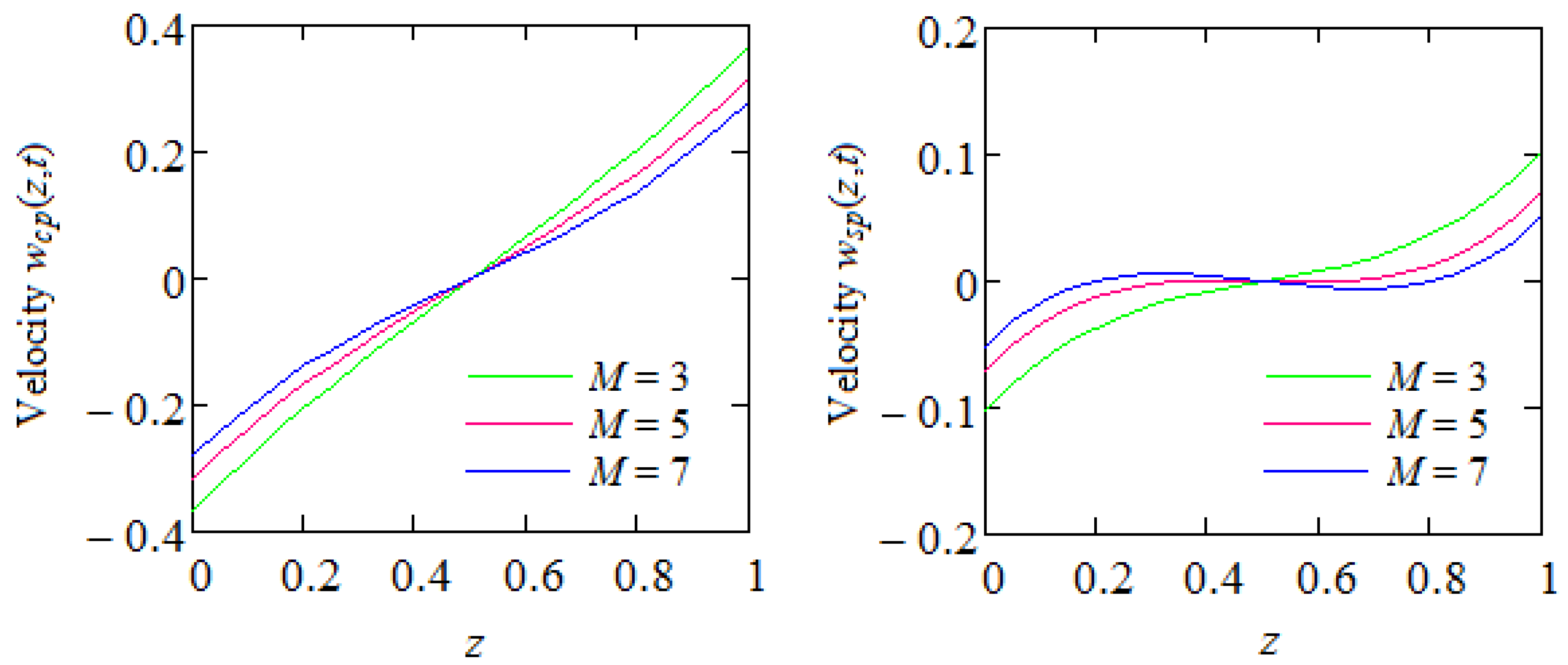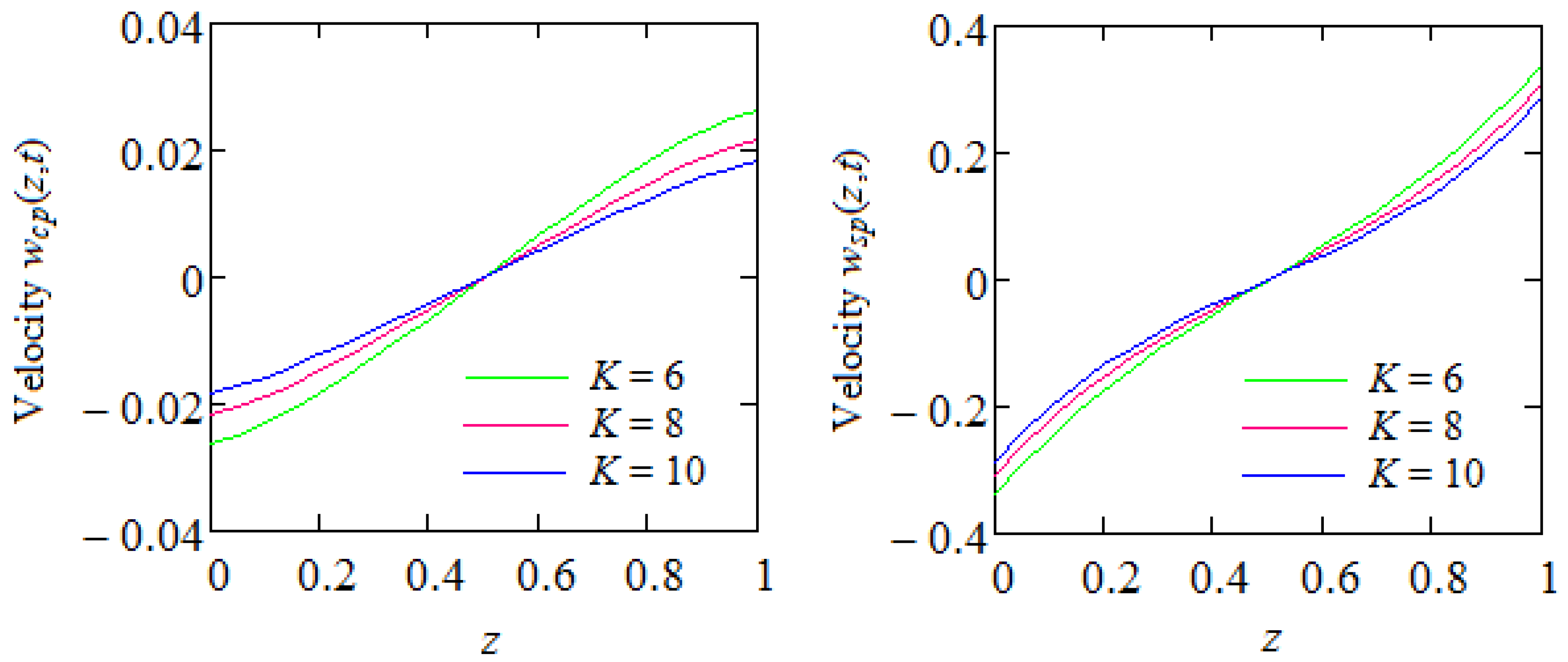K. In Figure 1 and Figure 2, for comparison, are close presented the variations of the dimensionless steady state velocities $w_{cp}(z,t)$ and $w_{sp}(z,t)$ against z for a fixed value of M and increasing values of K, respectively, for a fixed value of K and increasing values of M.

In all cases, the fluid velocities have a sign in the upper half of the channel and opposite sign in the other half. However, in absolute value, the fluid velocities are equal in points located at equal distances from the plates. This important result certificates the fact that the volume flux across a plane vertical to the direction motion per unit width of that plane is zero.

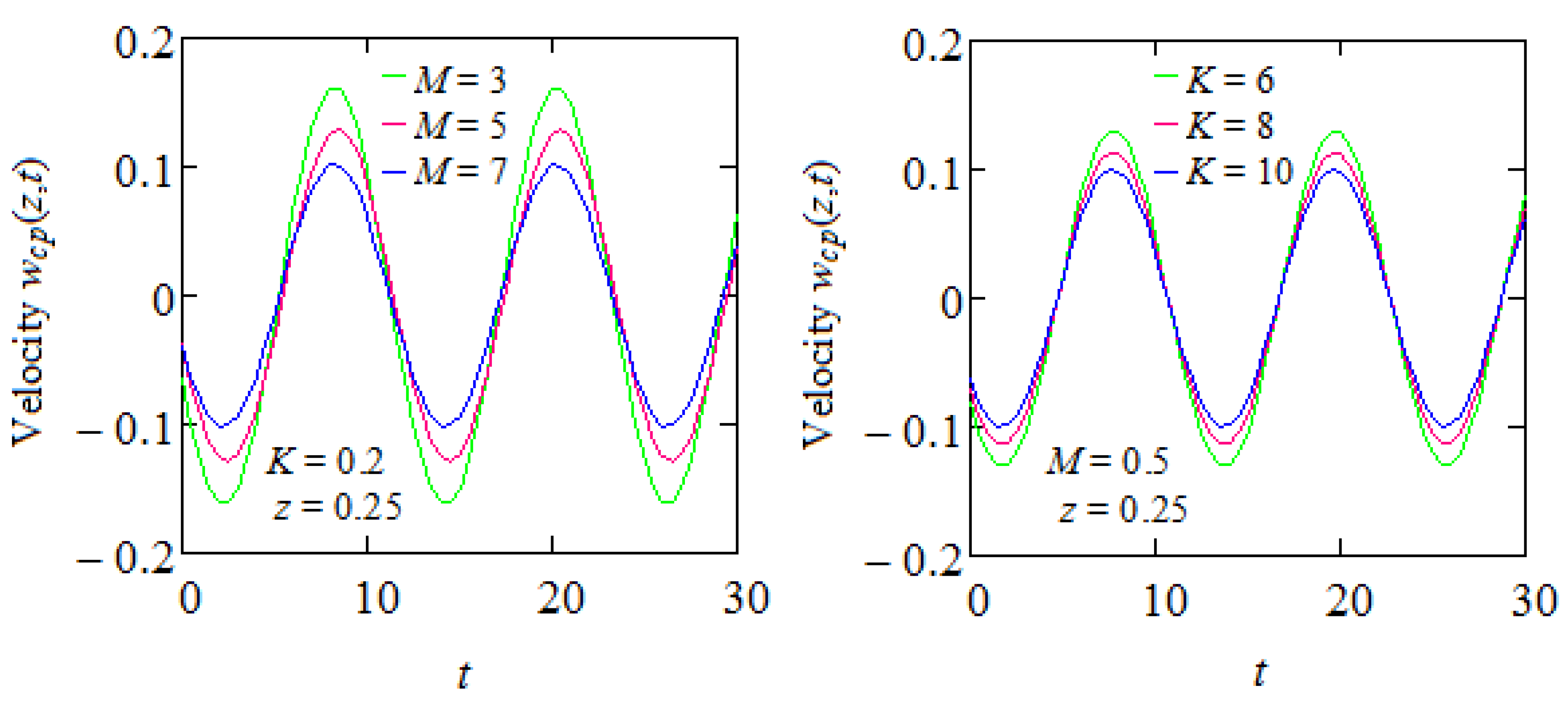
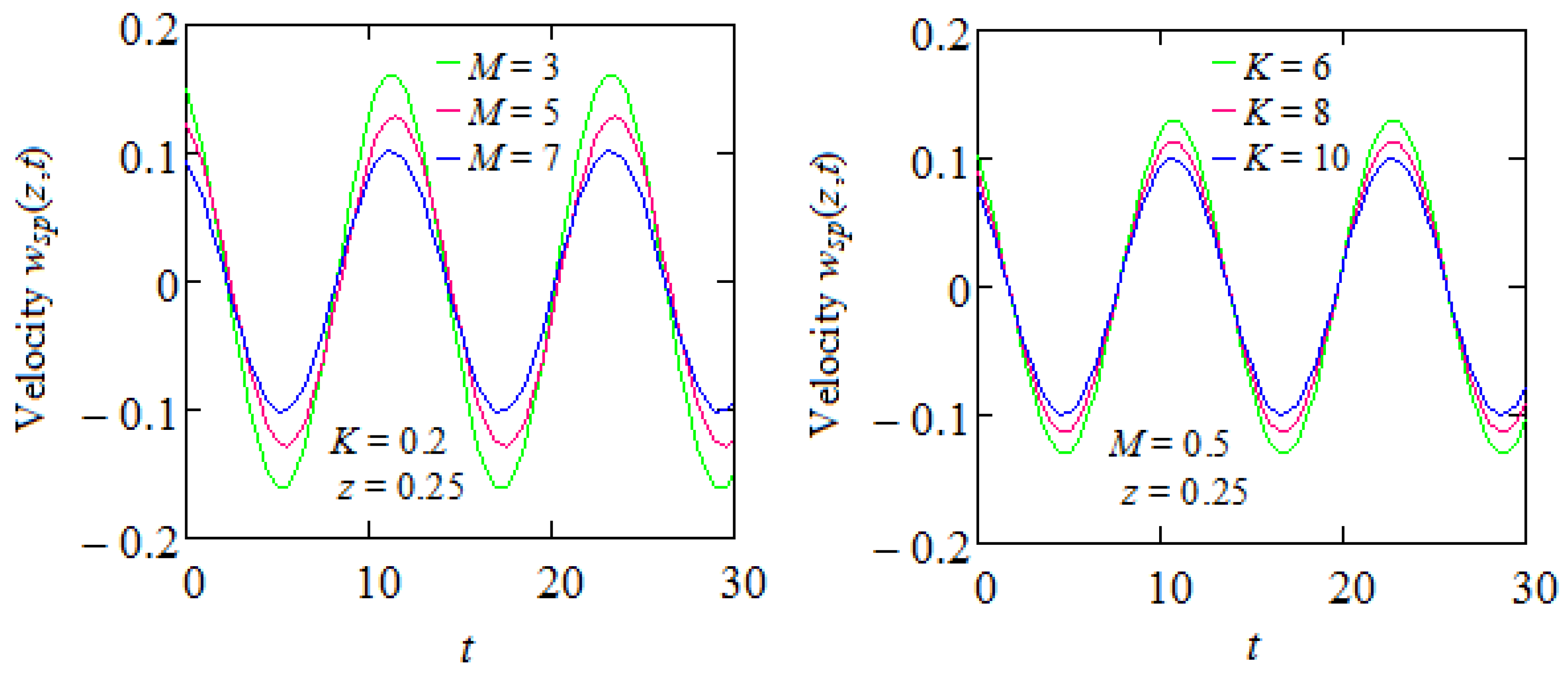
The variations in time of the two steady velocities $w_{cp}(z,t)$ and $w_{sp}(z,t)$ (given by the same Equations (27) and (28)) in the plane $z=1/4$ are depicted in Figure 3 and Figure 4 for increasing values of the magnetic and porous parameters M and K. The oscillatory behavior of the two motions, as well as the phase difference between them, is easily observable. In addition, as it was to be expected from previous results, the amplitude of oscillations declines for increasing values of M or K. Furthermore, the oscillations’ amplitudes of the two motions are identical at equal values of the two parameters M and K.

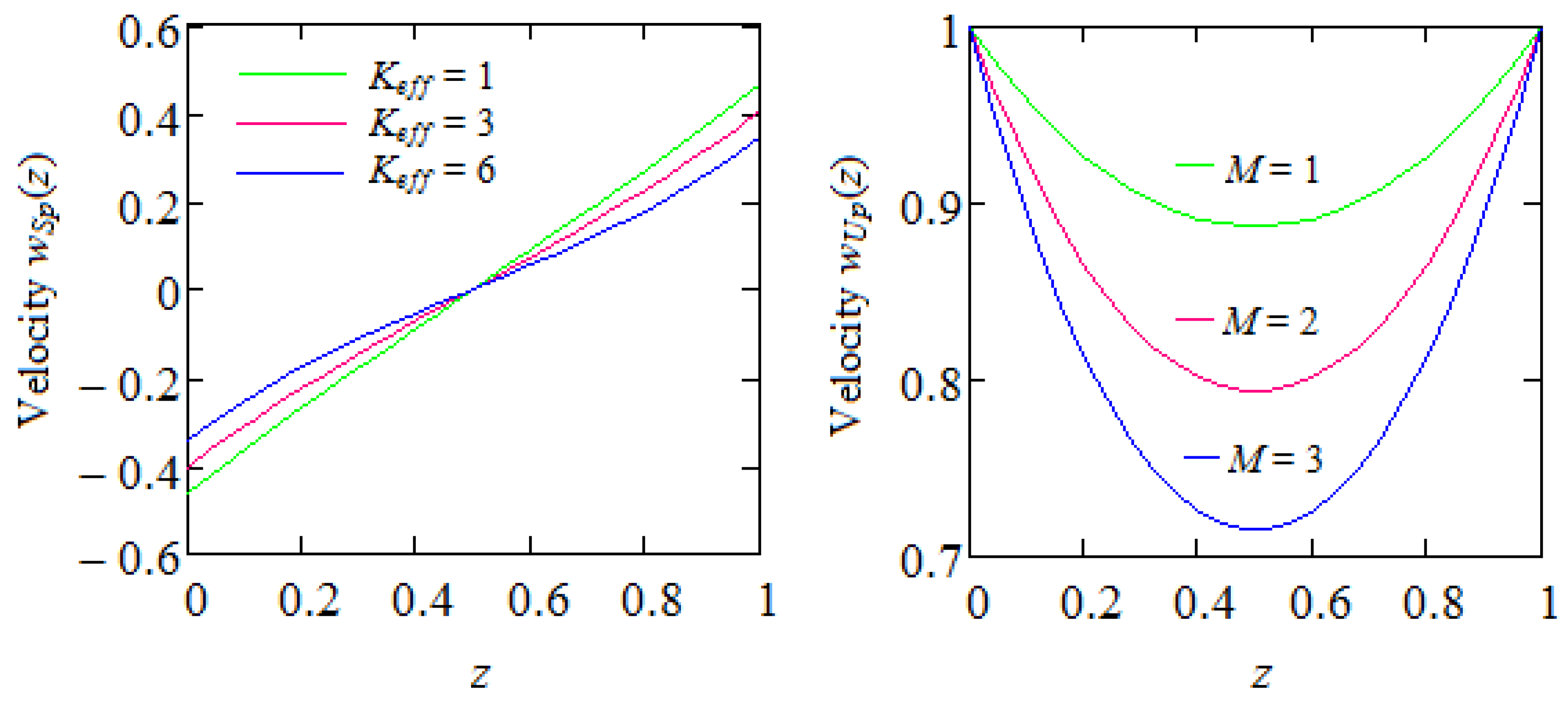
Now, for comparison, diagrams of dimensionless steady velocities $w_{Sp}(z)$ and $w_{Up}(z)$ are depicted adjoining in Figure 5 for increasing values of $K_{eff}$ and M, respectively. They correspond to motions of incompressible Newtonian and rate type fluids between two infinite horizontal parallel plates which apply a constant shear stress to the fluid or move in their planes with the constant velocity U. The difference between their graphical representations is essential. First of all, the velocity $w_{Sp}(z)$ has positive values in the upper half of the channel and negative values in the lower part but their absolute values are equal at the same distances from the midplane $z=1/2$. The second velocity field $w_{Up}(z)$, as expected, has positive values on the entire flow domain, is symmetric with respect to the plane $z=1/2$ and satisfies the boundary conditions. However, both $w_{Sp}(z)$ and $w_{Up}(z)$ in absolute value are decreasing functions with respect to the parameters $K_{eff}$ or M, respectively. It means that the fluid flows slower in the presence of a magnetic field or porous medium.

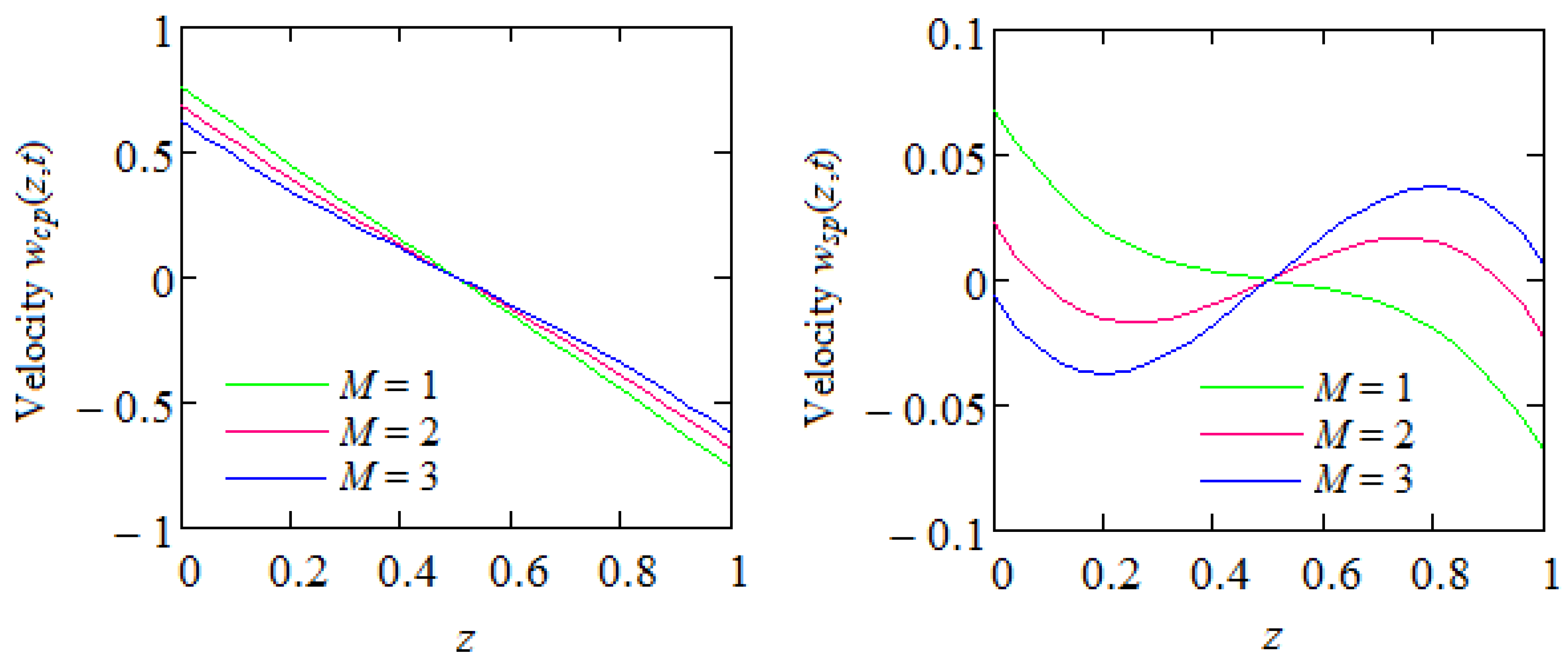
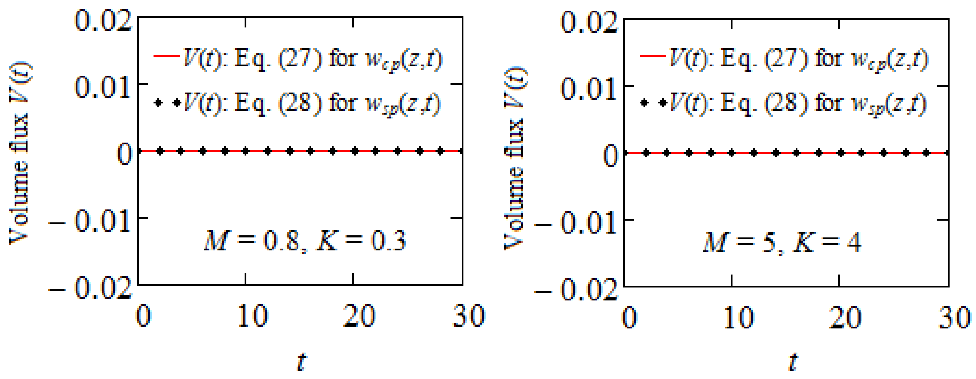
Finally, for a new graphical confirmation concerning the zero value of the volume flux across a plane orthogonal to the flow direction, we include here Figure 6 for the steady velocity fields $w_{cp}(z,t)$ and $w_{sp}(z,t)$ given by Equations (48) and (50). From these graphs it follows that the volume flux on a plane perpendicular to the flow direction is zero both for motions in which a differential expression of shear stress is prescribed on boundary and motions with shear stresses on the boundary. This result is also brought to light by means of Figure 7 for the most general velocity fields $w_{cp}(z,t)$ and $w_{sp}(z,t)$ corresponding to motions of IGBFs with a differential expression of the shear stress prescribed on the boundary.

The main results that have been obtained in this paper are the following:

-

Analytical expressions are provided for the dimensionless steady state solutions of some MHD motions of IGBFs through a porous medium between infinite horizontal parallel plates when a differential expression of shear stress is prescribed on boundary.

-

Volume flux across a plane orthogonal to the flow direction per unit width of that plane, contrary to our expectations, is zero for isothermal motions of IGBFs in which shear stress or a differential expression of shear stress is prescribed on plates having equal values.

-

The governing equations for fluid velocity and shear stress in MHD motions of IGBSs between parallel plates have identical forms. Consequently, any MHD motion problem of IGBFs in such a domain or over an infinite plate can be solved when shear stress is prescribed on the boundary.

-

The steady velocity $w_{Sp}(z)$ and the shear stress ${\eta }_{Sp}(z)$ corresponding to the motion of IGBFs due to a constant shear stress on the boundary do not depend independently on the magnetic and porous parameters M and K. Therefore, a two parameter approach for these entities is superfluous.

-

An IGBF flows slower in the presence of a magnetic field or porous medium.