Four Measures of Association and Their Representations in Terms of Copulas

Abstract

Four measures of association, namely, Spearman’s $\rho$, Kendall’s $\tau$, Blomqvist’s $\beta$ and Hoeffding’s ${\mathsf{\Phi }}^2$, are expressed in terms of copulas. Conveniently, this article also includes explicit expressions for their empirical counterparts. Moreover, copula representations of the four coefficients are provided for the multivariate case, and several specific applications are pointed out. Additionally, a numerical study is presented with a view to illustrating the types of relationships that each of the measures of association can detect.

1. Introduction

Copula representations and sample estimates of the correlation measures attributed to Spearman, Kendall, Blomqvist and Hoeffding are provided in this paper. All these measures of association depend on the ranks of the observations on each variable. They can reveal the strength of the dependence between two variables that are not necessarily linearly related, as is required in the case of Pearson’s correlation. They can as well be applied to ordinal data. While the Spearman, Kendall and Blomqvist measures of association are suitable for observations exhibiting monotonic relationships, Hoeffding’s index can also ascertain the extent of the dependence between the variables, regardless of the patterns that they may follow. Thus, these four measures of association prove quite versatile when it comes to assessing the strength of various types of relationships between variables. Moreover, since they are rank-based, they are all robust with respect to outliers. What is more, they can be readily evaluated.

Copulas are principally utilized for modeling dependency features in multivariate distributions. They enable one to represent the joint distribution of two or more random variables in terms of their marginal distributions and a specific correlation structure. Thus, the effect of the dependence between the variables can be separated from the contribution of each marginal. As measures of dependence, copulas have found applications in numerous fields of scientific investigations, including reliability theory, signal processing, geodesy, hydrology, finance and medicine. We now review certain basic definitions and results on the subject.

In the bivariate framework, a copula function is a distribution whose support is the unit square ${\mathbb{1}}^2={[0,1]}^2$ and whose marginals are uniformly distributed. A more formal definition is now provided.

A function $C:{\mathbb{1}}^2\mapsto \mathbb{1}$ is a bivariate copula if it satisfies the two following properties:

• For every $u,v\in \mathbb{1}$,

  $$\begin{array}{c}\hfill C(u,1)=u,C(1,v)=v,\mathrm{and}C(u,0)=C(0,v)=0.\end{array}$$
• For every $u_1,u_2,v_1,v_2\in \mathbb{1}$ such that $u_1\le u_2$ and $v_1\le v_2$,

  $$C(u_2,v_2)-C(u_2,v_1)-C(u_1,v_2)+C(u_1,v_1)\ge 0.$$

This last inequality implies that $C(u,v)$ is increasing in both variables.

We now state a result due to Sklar (Theorem 1) [1].

Theorem 1. 

Let $H(x,y)$ be the joint cumulative distribution function of the random variables X and Y whose continuous marginal distribution functions are denoted by $F\left(x\right)$ and $G\left(y\right)$. Then, there exists a unique bivariate copula $C:{\mathbb{1}}^2\mapsto$$\mathbb{1}$ such that

$$H(x,y)=C\left(F\left(x\right),G\left(y\right)\right)$$

(1)

where $C(·,·)$ is a joint cumulative distribution function having uniform marginals. Conversely, for any continuous cumulative distribution functions $F\left(x\right)$ and $G\left(y\right)$ and any copula $C(·,·)$, the function $H(·,·)$, as defined in (1), is a joint distribution function with marginal distribution functions $F(·)$ and $G(·)$.

Sklar’s theorem provides a technique for constructing copulas. Indeed, the function

$$C(u,v)=H\left(F^{-1}\left(u\right),G^{-1}\left(v\right)\right)$$

(2)

is a bivariate copula, where the quasi-inverses $F^{-1}(·)$ and $G^{-1}(·)$ are defined by

$$F^{-1}\left(u\right)=inf\left\{x\right|F\left(x\right)\ge u\},u\in (0,1),$$

(3)

and

$$G^{-1}\left(v\right)=inf\left\{y\right|G\left(y\right)\ge v\},v\in (0,1).$$

(4)

Copulas are invariant with respect to strictly increasing transformations. More specifically, assuming that X and Y are two continuous random variables whose associated copula is $C(·,·)$, and letting $\alpha (·)$ and $\beta (·)$ be two strictly increasing functions and $C_{\alpha ,\beta }(·,·)$ be the copula obtained from $\alpha \left(X\right)$ and $\beta \left(Y\right)$, then for all $(u,v)\in {\mathbb{1}}^2,$ one has

$$C_{\alpha ,\beta }(u,v)=C(u,v).$$

(5)

We shall denote the probability density function corresponding to the copula $C(u_1,u_2)$ by

$$c(u,v)=\frac{{\partial }^2}{\partial u\partial v}C(u,v).$$

(6)

The following relationship between $h(·,·)$, the joint density function of the random variables X and Y as defined in Sklar’s theorem, and the associated copula density function $c(·,·)$ can then be readily obtained from Equation (1) as

$$h(x,y)=f\left(x\right)g\left(y\right)c\left(F\right(x),G(y\left)\right)$$

(7)

where $f\left(x\right)$ and $g\left(y\right)$ denote the marginal density functions of X and Y, respectively. Accordingly, a copula density function can be expressed as follows:

$$c(u,v)=\frac{h(F^{-1}\left(u\right),G^{-1}\left(v\right))}{f\left(F^{-1}\left(u\right)\right)g\left(G^{-1}\left(v\right)\right)}.$$

(8)

Now, given a random sample $(x_1,y_1),\dots ,(x_n,y_n)$ generated from the continuous random vector $(X,Y)$, let

$$(u_i,v_i)=(F\left(x_i\right),G\left(y_i\right)),i=1,\dots ,n,$$

(9)

where $F(·)$ and $G(·)$ are the usually unknown marginal cumulative distribution functions (cdfs) of X and Y. The empirical marginal cdfs $\widehat{F}(·)$ and $\widehat{G}(·)$ are then utilized to determine the pseudo-observations:

$$({\widehat{u}}_i,{\widehat{v}}_i)=(\widehat{F}\left(x_i\right),\widehat{G}\left(y_i\right)),i=1,\dots ,n,$$

(10)

where the empirical cdfs (ecdfs) are given by $\widehat{F}\left(x\right)=\frac{1}{n}{\sum }_{i=1}^n\mathcal{I}(x_i\le x)$ and $\widehat{G}\left(y\right)=\frac{1}{n}{\sum }_{i=1}^n\mathcal{I}(y_i\le y)$, with $\mathcal{I}(\aleph )$ denoting the indicator function which is equal to one if the condition ℵ is verified and zero, otherwise. Equivalently, one has

$$({\widehat{u}}_i,{\widehat{v}}_i)=(r_i/n,s_i/n),$$

(11)

where $r_i$ is the rank of $x_i$ among $\{x_1,\dots ,x_n\}$, and $s_i$ is the rank of $y_i$ among $\{y_1,\dots ,y_n\}$.

The frequencies or probability mass function of an empirical copula can be expressed as

$$\begin{array}{cc}\hfill \widehat{c}(u,v)& =\frac{1}{n}\sum _{i=1}^n\mathcal{I}(\widehat{F}\left(x_i\right)=u)\mathcal{I}(\widehat{G}\left(y_i\right)=v)\hfill \\ \hfill & =\frac{1}{n}\sum _{i=1}^n\mathcal{I}(r_i/n=u)\mathcal{I}(s_i/n=v),\hfill \end{array}$$

(12)

and the corresponding empirical copula (distribution function) is then given by

$$\begin{array}{cc}\hfill \widehat{C}(u,v)& =\frac{1}{n}\sum _{i=1}^n\mathcal{I}(\widehat{F}\left(x_i\right)\le u)\mathcal{I}(\widehat{G}\left(y_i\right)\le v)\hfill \\ \hfill & =\frac{1}{n}\sum _{i=1}^n\mathcal{I}(r_i/n\le u)\mathcal{I}(s_i/n\le v),\hfill \end{array}$$

(13)

which is a consistent estimate of $C(u,v)$. We note that, in practice, the ranks are often divided by $n+1$ instead of n in order to mitigate certain boundary effects, and that other adjustments that are specified in Section 2 may also be applied. As pointed out by [2], who refers to [3], “Empirical copulas were introduced and first studied by Deheuvels who called them empirical dependence functions”.

Additional properties of copulas that are not directly relevant to the results presented in this article are discussed for instance in [4,5,6].

This article contains certain derivations that do not seem to be available in the literature and also provides missing steps that complete the published proofs. It is structured as follows: Section 2, Section 3, Section 4 and Section 5, which, respectively, focus on Spearman’s, Kendall’s, Blomqvist’s and Hoeffding’s correlation coefficients, include representations of these measures of dependence in terms of copulas, in addition to providing sample estimates thereof and pointing out related distributional results of interest. The effectiveness of these correlation coefficients in assessing the trends present in five data sets exhibiting distinctive patterns is assessed in a numerical study that is presented in Section 6. Section 7 is dedicated to multivariate extensions of the four measures of association and their copula representations.

To the best of our knowledge, the four major dependence measures discussed here, along with their representations in terms of copulas, have not been previously covered in a single source.

2. Spearman’s Rank Correlation

Spearman’s rank correlation statistic, also referred to as Spearman’s $\rho$, measures the extent to which the relationship between two variables is monotonic—either increasing or decreasing.

First, Spearman’s $\rho$ is expressed in terms of a copula denoted by $C(U,V)$. Then, some equivalent representations of Spearman’s rank correlation statistic are provided; one of them is obtained by replacing $C(U,V)$ by its empirical counterpart.

Let $(X,Y)$ be a bivariate continuous random vector having $h(x,y)$ as its joint density function, and $F\left(X\right)$ and $G\left(Y\right)$ denote the respective marginal distribution functions of X and Y.

Theoretically, Spearman’s correlation is given by

$$\begin{array}{cc}\hfill {\rho }_S& =\frac{Cov\left[F\right(X),G(Y\left)\right]}{\sqrt{Var\left[F\right(X\left)\right]Var\left[G\right(Y\left)\right]}}\hfill \end{array}$$

(14)

$$\begin{array}{cc}\hfill & =\frac{{\int \int }_{{\mathbb{R}}^2}F\left(x\right)G\left(y\right)h(x,y)\mathrm{d}x\mathrm{d}y-\left({\int }_{\mathbb{R}}F\left(x\right)\mathrm{d}F\left(x\right)\right)\left({\int }_{\mathbb{R}}G\left(y\right)\mathrm{d}G\left(y\right)\right)}{\sqrt{[{\int }_{\mathbb{R}}F{\left(x\right)}^2\mathrm{d}F\left(x\right)-\left({\int }_{\mathbb{R}}{\left(F\left(x\right)\mathrm{d}F\left(x\right)\right)}^2\right][{\int }_{\mathbb{R}}G{\left(y\right)}^2\mathrm{d}G\left(y\right)-\left({\int }_{\mathbb{R}}{\left(G\left(y\right)\mathrm{d}G\left(y\right)\right)}^2\right]}}\hfill \end{array}$$

(15)

$$\begin{array}{cc}\hfill & =\frac{{\int }_0^1{\int }_0^{1}uvc(u,v)\mathrm{d}u\mathrm{d}v-(1/2)(1/2)}{\sqrt{(1/12)(1/12)}}\mathrm{in}\mathrm{light}\mathrm{of}\left(8\right),\hfill \end{array}$$

(16)

$\begin{array}{cc}\hfill & \mathrm{with}\mathrm{the}\mathrm{transformation}\{x=F^{-1}\left(u\right)\mathrm{and}y=G^{-1}\left(v\right)\}\mathrm{whose}\mathrm{Jacobian}\mathrm{is}\mathrm{the}\hfill \\ \hfill & \mathrm{inverse}\mathrm{of}\mathrm{the}\mathrm{Jacobian}\mathrm{associated}\mathrm{with}\mathrm{the}\mathrm{following}\mathrm{transformation}:\hfill \end{array}$

$$\begin{array}{c}\hfill \{u=F\left(x\right)\mathrm{and}v=G\left(y\right)\},\mathrm{that}\mathrm{is},1/\left[f\left(F^{-1}\left(u\right)\right)g\left(G^{-1}\left(v\right)\right)\right],\end{array}$$

$$\begin{array}{cc}\hfill & =12{\int }_0^1{\int }_0^{1}C(u,v)\mathrm{d}u\mathrm{d}v-3,\hfill \end{array}$$

(17)

$$\begin{array}{cc}\hfill & =12E\left[UV\right]-3,\hfill \end{array}$$

(18)

where $C(·,·)$ and $c(·,·)$, respectively, denote the copula and copula density function associated with $(X,Y)$, and $\mathbb{R}$ represents the set of real numbers. In [7,8], it is taken as a given that the double integral appearing in (16) can be expressed as that appearing in (17). We now prove that this is indeed the case. First, recall that $\frac{{\partial }^{2}C(u,v)}{\partial u\partial v}=c(u,v)$, the copula density function. On integrating by parts twice, one has

$$\begin{array}{cc}\hfill {\int }_0^1{\int }_0^{1}uv\mathrm{d}C(u,v)& ={\int }_0^1{\int }_0^{1}uv\frac{{\partial }^{2}C(u,v)}{\partial u\partial v}\mathrm{d}v\mathrm{d}u\hfill \\ \hfill & ={\int }_0^{1}u\left[{\int }_0^{1}v\frac{\partial }{\partial v}\left(\frac{\partial C(u,v)}{\partial u}\right)\mathrm{d}v\right]\mathrm{d}u\hfill \\ \hfill & ={\int }_0^{1}u\left[v{\left.\frac{\partial C(u,v)}{\partial u}\right|}_0^1-{\int }_0^1\frac{\partial C(u,v)}{\partial u}\mathrm{d}v\right]\mathrm{d}u\hfill \\ \hfill & ={\int }_0^{1}u\left[1-{\int }_0^1\frac{\partial C(u,v)}{\partial u}\mathrm{d}v\right]\mathrm{d}u,\mathrm{as}C(u,1)=u\hfill \\ \hfill & ={\int }_0^{1}u\mathrm{d}u-{\int }_0^1{\int }_0^{1}u\frac{\partial C(u,v)}{\partial u}\mathrm{d}v\mathrm{d}u\hfill \\ \hfill & =\frac{1}{2}-{\int }_0^1\left[uC(u,v){|}_0^1-{\int }_0^{1}C(u,v)\mathrm{d}u\right]\mathrm{d}v\hfill \\ \hfill & =\frac{1}{2}-\frac{1}{2}+{\int }_0^1{\int }_0^{1}C(u,v)\mathrm{d}u\mathrm{d}v,\mathrm{as}C(1,v)=v\hfill \\ \hfill & ={\int }_0^1{\int }_0^{1}C(u,v)\mathrm{d}u\mathrm{d}v.\hfill \end{array}$$

(19)

Now, let $(X_1,Y_1),\dots ,(X_n,Y_n)$ be a random sample generated from the random vector $(X,Y)$, and denote by $\widehat{F}\left(X\right)$ and $\widehat{G}\left(Y\right)$ the respective empirical distribution functions of X and Y. Throughout this article, the sample size is assumed to be n. On denoting by $R_i$ and $S_j$, the rank of $X_i$ among $\{X_1,\dots ,X_n\}$ and the rank of $Y_j$ among $\{Y_1,\dots ,Y_n\}$, respectively, one has $\widehat{F}\left(X_i\right)=R_i/n\equiv U_i$ and $\widehat{G}\left(Y_j\right)=S_j/n\equiv V_j$, where $U_i$ and $V_j$ denote the canonical pseudo-observations on each component. Note that the rank averages $\overline{R}$ and $\overline{S}$ are both equal to $(n+1)/2$. Then, Spearman’s rank correlation estimator admits the following equivalent representations:

$$\begin{array}{cc}\hfill {\widehat{\rho }}_S& =\frac{{\sum }_{i=1}^n(R_i-\overline{R})(S_i-\overline{S})}{\sqrt{{\sum }_{i=1}^n{(R_i-\overline{R})}^2{\sum }_{i=1}^n{(S_i-\overline{S})}^2}}\hfill \end{array}$$

(20)

$$\begin{array}{cc}\hfill & =\frac{\left({\sum }_{i=1}^n{R}_i{S}_i\right)-n\overline{R}\overline{S}}{\sqrt{[\left({\sum }_{i=1}^n{R}_i^2\right)-n{\overline{R}}^2][\left({\sum }_{i=1}^n{S}_i^2\right)-n{\overline{S}}^2)]}}\hfill \end{array}$$

(21)

$$\begin{array}{cc}\hfill & =\frac{\left({\sum }_{i=1}^n\widehat{F}\left(x_i\right)\widehat{G}\left(y_i\right)\right)-n{(n+1)}^2/4}{\sqrt{[\left({\sum }_{i=1}^n\widehat{F}{\left(x_i\right)}^2\right)-n{(n+1)}^2/4][\left({\sum }_{i=1}^n\widehat{G}{\left(y_i\right)}^2\right)-n{(n+1)}^2/4]}}\hfill \end{array}$$

(22)

$$\begin{array}{cc}\hfill & =\frac{\left({\sum }_{i=1}^n{U}_i{V}_i\right)-n{(n+1)}^2/4}{\sqrt{[\left({\sum }_{i=1}^n{U}_i^2\right)-n{(n+1)}^2/4][\left({\sum }_{i=1}^n{V}_i^2\right)-n{(n+1)}^2/4]}}\hfill \end{array}$$

(23)

$$\begin{array}{cc}\hfill & =\frac{{\sum }_{i=1}^n(U_i-\overline{U})(V_i-\overline{V})}{\sqrt{{\sum }_{i=1}^n{(U_i-\overline{U})}^2{\sum }_{i=1}^n{(V_i-\overline{V})}^2}},\hfill \end{array}$$

(24)

where $\overline{U}={\sum }_{i=1}^n{U}_i/n$ and $\overline{V}={\sum }_{i=1}^n{V}_i/n$.

Of course, (24) readily follows from (20), and it is seen from either one of these expressions that Spearman’s rank correlation is not be affected by any monotonic affine transformation, whether applied to the ranks or the canonical pseudo-observations. As pointed out for instance in [9], the pseudo-observations are frequently taken to be

$${\widehat{U}}_i=\frac{R_i}{n+1}=\frac{n}{n+1}\widehat{F}\left(x_i\right)=\frac{1}{n+1}\sum _{k=1}^n\mathcal{I}(x_k\le x_i)$$

(25)

and

$${\widehat{V}}_j=\frac{S_j}{n+1}=\frac{n}{n+1}\widehat{G}\left(y_j\right)=\frac{1}{n+1}\sum _{k=1}^n\mathcal{I}(y_k\le y_j).$$

(26)

Alternatively, one can define the pseudo-observations so that they be uniformly—and less haphazardly—distributed over the unit interval as follows:

$$\widetilde{U_i}=\frac{R_i}{n}-\frac{1}{2n}=\widehat{F}\left(x_i\right)-\frac{1}{2n}$$

(27)

and

$$\widetilde{V_j}=\frac{S_j}{n}-\frac{1}{2n}=\widehat{G}\left(y_j\right)-\frac{1}{2n}.$$

(28)

In a simulation study, Dias (2022) [10] observed that such pseudo-observations have a lower bias than those obtained by dividing the ranks by $n+1$. What is more, it should be observed that if we extend the pseudo-observations ${\tilde{U}}_i,i=1,\dots ,n,$ and ${\tilde{V}}_j,j=1,\dots ,n,$ by $\frac{1}{2n}$ on each side and assign their respective probability, namely, $\frac{1}{n}$, to each of the n resulting subintervals, the marginal distributions is then uniformly distributed within the interval $[0,1]$, which happens to be a requirement for a copula density function. However, this is not the case for any other affine transformation of the ranks. The alternative transformations $\frac{\mathrm{rank}-1/3}{n+1/3}$ and $\frac{\mathrm{rank}-1}{n-1}$ were also considered by [10,11], respectively. As established in [10], the pseudo-observation estimators resulting from any of the above-mentioned transformations as well as the canonical pseudo-observations are consistent estimators of the underlying distribution functions.

Kojanovik and Yan (2010) [7] pointed out that ${\widehat{\rho }}_S$, as specified in (21), can also be expressed as

$${\widehat{\rho }}_S=\frac{12}{n(n+1)(n-1)}\sum _{i=1}^n{R}_i{S}_i-3\frac{(n+1)}{(n-1)},$$

(29)

where ${\widehat{\rho }}_S$ is a consistent estimator of ${\rho }_S$.

Moreover, it can be algebraically shown that, alternatively,

$${\widehat{\rho }}_S=1-6\sum _{i=1}^n\frac{{(R_i-S_i)}^2}{n(n^2-1)}$$

(30)

when the ranks are distinct integers.

On writing (17) as

$${\rho }_S=12{\int }_0^1{\int }_0^{1}uv\mathrm{d}C(u,v)-3,$$

(31)

and replacing $C(u,v)$ by $\widehat{C}(u,v)$ as defined in (13), the double integral becomes

$$\frac{1}{n}\sum _{i=1}^n{\int }_0^{1}u\mathrm{d}\left(\mathcal{I}(r_i/n\le u)\right){\int }_0^{1}v\mathrm{d}\left(\mathcal{I}(s_i/n\le v)\right).$$

For instance, on integrating the first integral by parts, one has

$$u\mathcal{I}(r_i/n\le u){|}_0^1-{\int }_0^1\mathcal{I}(r_i/n\le u)\mathrm{d}u=1-(1-r_i/n)=r_i/n.$$

Thus, the resulting estimator of Spearman’s rank correlation is given by

$${\widehat{\rho }}_S=\frac{12}{n^3}\sum _{i=1}^n{R}_i{S}_i-3,$$

which is approximately equal to that given in (29).

Now, letting $C_{\theta }(u,v)$ be a copula whose functional representation is known, and assuming that it is a one-to-one function of the dependence parameter $\theta$, it follows from (17) that

$${\rho }_S\left(\theta \right)=12{\int \int }_{{\mathbb{1}}^2}{C}_{\theta }(u,v)\mathrm{d}u\mathrm{d}v-3,$$

(32)

which provides an indication of the extent to which the variables are monotonically related. Moreover, since ${\widehat{\rho }}_S$, as defined in (21), (29) or (30), tends to ${\rho }_S\left(\theta \right)$, $\widehat{\theta }={\rho }_S^{-1}\left({\widehat{\rho }}_S\right)$ can serve as an estimate of $\theta$.

It follows from (17) that Spearman’s $\rho$ can be expressed as

$${\rho }_S=12{\int \int }_{{\mathbb{1}}^2}[C(u,v)-uv]\mathrm{d}u\mathrm{d}v.$$

(33)

On replacing $\left[C\right(u,v)-uv]$ in (33) by $\left|C\right(u,v)-uv|$, one obtains a measure based on the $L_1$ distance between the copula C and the product copula $\Pi =uv$ ( [5]). This is the so-called Schweizer–Wolff’s sigma as defined in [12], which is given by

$${\sigma }_{X,Y}={\sigma }_C=12{\int \int }_{{\mathbb{1}}^2}|C(u,v)-uv|\mathrm{d}u\mathrm{d}v.$$

(34)

The expression (34) is a measure of dependence which satisfies the properties of Rényi’s axioms [13] for measures of dependence [12], [14] (p. 145).

Note that Pearson’s correlation coefficient,

$$\widehat{r}=\frac{{\sum }_{i=1}^n(x_i-\overline{x})(y_i-\overline{y})}{\sqrt{{\sum }_{i=1}^n{(x_i-\overline{x})}^2{\sum }_{i=1}^n{(y_i-\overline{y})}^2}},$$

(35)

only measures the strength of a linear relationship between X and Y, whereas Spearman’s rank correlation ${\rho }_S$ assesses the strength of any monotonic relationship between X and Y. The latter is always well-defined, which is not the case for the former. Both vary between $-1$ and 1 and ${\rho }_S=\pm 1$ indicates that Y is either an increasing or a decreasing function of X. Moreover, it should be noted that Pearson’s correlation coefficient cannot be expressed in terms of copulas since its estimator is a function of the observations themselves rather than their ranks.

The next three sections include results that were gleaned from the following books among others: [4,5,15,16].

3. Kendall’s Rank Correlation Coefficient

Kendall’s $\tau$, also referred to as Kendall’s rank correlation coefficient, was introduced by [17]. Maurice Kendall also proposed an estimate thereof and published several papers as well as a monograph in connection with certain ordinal measures of correlation. Further historical details are available from [18].

Kendall’s $\tau$ is a nonparametric measure of association between two variables, which is based on the number of concordant pairs minus the number of discordant pairs. Consider two observations $(x_i,y_i)$ and $(x_j,y_j),$ with $(i,j)\in \{1,\dots ,n\}$ such that $i\ne j$, that are generated from a vector $(X,Y)$ of continuous random variables. Then, for any such assignment of pairs, define each pair as being concordant, discordant or equal, as follows:

○

$(x_i,y_i)$ and $(x_j,y_j)$ are concordant if

$\{x_i<x_j\mathrm{and}{y}_i<y_j\mathrm{or}\mathrm{if}{x}_i>x_j\mathrm{and}{y}_i>y_j\}$, or equivalently

$(x_i-x_j)(y_i-y_j)>0$, i.e., the slope of the line connecting the two points is positive.

○

$(x_i,y_i)$ and $(x_j,y_j)$ are discordant if

$\{x_i<x_j\mathrm{and}{y}_i>y_j\mathrm{or}\mathrm{if}{x}_i>x_j\mathrm{and}{y}_i<y_j\}$, or equivalently

$(x_i-x_j)(y_i-y_j)<0$, i.e., the slope of the line connecting the two points is negative.

○

$(x_i,y_i)\mathrm{and}(x_j,y_j)$ are equal if $x_i=x_j \mathrm{or} y_i=y_j$. Actually, pair equality can be disregarded as the random variables X and Y are assumed to be continuous.

3.1. The Empirical Kendall’s τ

Let $\{(x_1,y_1),(x_2,y_2),\dots ,(x_n,y_n)\}$ be a random sample of n pairs arising from the vector $(X,Y)$ of continuous random variables. There are $C_2^n=\left(\genfrac{}{}{0pt}{}{n}{2}\right)$ possible ways of selecting distinct pairs $(x_i,y_i)$ and $(x_j,y_j)$ of observations in the sample, with each pair being either concordant or discordant.

Let $S_{ij}$ be defined as follows:

$$S_{ij}=\mathrm{sign}(X_i-X_j)\mathrm{sign}(Y_i-Y_j),$$

(36)

where

$$\mathrm{sign}\left(u\right)=\left\{\begin{array}{cccc}\hfill -& 1\hfill & \hfill \mathrm{if}& u<0\hfill \\ \hfill & 0\hfill & \hfill \mathrm{if}& u=0\hfill \\ \hfill & 1\hfill & \hfill \mathrm{if}& u>0.\hfill \end{array}\right.$$

Then, the values that $S_{ij}$ can take on are

$$s_{ij}=\left\{\begin{array}{ccc}\hfill -& 1\hfill & \hfill \mathrm{when}\mathrm{the}\mathrm{pairs}\mathrm{are}\mathrm{discordant}\\ \hfill & 0\hfill & \hfill \mathrm{when}\mathrm{the}\mathrm{pairs}\mathrm{are}\mathrm{neither}\mathrm{concordant}\mathrm{nor}\mathrm{discordant}\\ \hfill & 1\hfill & \hfill \mathrm{when}\mathrm{the}\mathrm{pairs}\mathrm{are}\mathrm{concordant}.\end{array}\right.$$

Kendall’s sample $\widehat{\tau }$ is defined as follows:

$$\widehat{\tau }=\sum _{1\le i<j\le n}\frac{s_{ij}}{C_2^n}=\frac{2}{n(n-1)}\sum _{1\le i<j\le n}{s}_{ij}.$$

(37)

Alternatively, on letting c denote the number of concordant pairs and d the number of discordant pairs in a given sample of size n, one can express the estimate of Kendall’s $\tau$ as

$$\widehat{\tau }=\frac{c-d}{c+d}=\frac{c-d}{C_2^n}=\frac{2(c-d)}{n(n-1)}.$$

(38)

As it is assumed that there can be no equality between pairs, $C_2^n=c+d$, so that

$$\widehat{\tau }=\frac{4c}{n(n-1)}-1\mathrm{or},\mathrm{equivalently},\widehat{\tau }=1-\frac{4d}{n(n-1)}.$$

(39)

In fact, $\widehat{\tau }$ is an unbiased estimator of $\tau$. As well, Kendall and Gibbons (1990) [19] (Chapter 5) established that Var$\left(\widehat{\tau }\right)=\frac{2(2n+5)}{9n(n-1)}$. A coefficient related to that specified in (39) was discussed in [20,21,22] in the context of double time series.

3.2. The Population Kendall’s τ

Letting $(X_1,Y_1)$ and $(X_2,Y_2)$ be independent and identically distributed random vectors, with the joint distribution function of $(X_i,Y_i)$ being $H(x,y)$, $F\left(x\right)$ and $G\left(y\right)$ denote the respective distribution functions of $X_i$ and $Y_j$, $i,j=1,2,$ and the associated copula be $C(u,v)=H(F^{-1}\left(u\right),G^{-1}\left(v\right))$, the population Kendall’s $\tau$ is defined as follows:

$$\begin{array}{cc}\hfill \tau & ={\tau }_{X,Y}=\mathrm{Pr}[\mathrm{concordant}\mathrm{pairs}]-\mathrm{Pr}[\mathrm{discordant}\mathrm{pairs}]\hfill \\ \hfill & \equiv p_c-p_d\hfill \end{array}$$

$$\begin{array}{cc}\hfill & =\mathrm{Pr}[(X_1-X_2)(Y_1-Y_2)>0]-\mathrm{Pr}[(X_1-X_2)(Y_1-Y_2)<0]\hfill \end{array}$$

(40)

$$\begin{array}{cc}\hfill & =2\mathrm{Pr}[(X_1-X_2)(Y_1-Y_2)>0]-1\hfill \end{array}$$

(41)

$$\begin{array}{cc}\hfill & =4\mathrm{Pr}\left[(X_1<X_2,Y_1<Y_2)\right]-1\hfill \end{array}$$

(42)

$$\begin{array}{cc}\hfill & =4{\int \int }_{{\mathbb{R}}^2}\mathrm{Pr}(X_2\le x,Y_2\le y)\mathrm{d}H(x,y)-1,\mathrm{with}H(x,y)=C(F\left(x\right),G\left(y\right))\hfill \end{array}$$

(43)

$$\begin{array}{cc}\hfill & =4{\int \int }_{{\mathbb{R}}^2}H(x,y)c(F\left(x\right),G\left(y\right))f\left(x\right)g\left(y\right)\mathrm{d}x\mathrm{d}y-1\hfill \\ \hfill & =4{\int \int }_{{\mathbb{1}}^2}\frac{H(F^{-1}\left(u\right),G^{-1}\left(v\right))c(u,v)f\left(F^{-1}\left(u\right)\right)g\left(G^{-1}\left(v\right)\right)}{f\left(F^{-1}\left(u\right)\right)g\left(G^{-1}\left(v\right)\right)}\mathrm{d}u\mathrm{d}v-1\hfill \end{array}$$

$$\begin{array}{cc}\hfill & =4{\int }_0^1{\int }_0^{1}C(u,v)\mathrm{d}C(u,v)-1\hfill \end{array}$$

(44)

$$\begin{array}{cc}\hfill & =4\mathrm{E}\left[C\right(U,V\left)\right]-1,\hfill \end{array}$$

(45)

where

$U\mathrm{and}V$ have a Uniform $(0,1)$ distribution, their joint cdf being $C(u,v)$;

$u=F_X\left(x\right)$ and $v=F_Y\left(y\right)$;

${\mathbb{R}}^2\equiv \left\{(x,y)\right|x\mathrm{and}y\mathrm{are}\mathrm{real}\mathrm{numbers}\}$;

$\mathrm{d}C(u,v)=\frac{{\partial }^{2}C(u,v)}{\partial u\partial v}\mathrm{d}u\mathrm{d}v=c(u,v)\mathrm{d}u\mathrm{d}v$.

Clearly, (41) follows from (40) since

$$\mathrm{Pr}[(X_1-X_2)(Y_1-Y_2)<0]=1-\mathrm{Pr}[(X_1-X_2)(Y_1-Y_2)>0].$$

We now state Theorem 5.1.1 from [5]:

Theorem 2. 

Let $(X_1,Y_1)$ and $(X_2,Y_2)$ be independent vectors of continuous random variables with joint distributions functions $H_1$ and $H_2$, respectively, with common marginals $F(·)$ and $G(·)$. Let $C_1$ and $C_2$ be the copulas of $(X_1,Y_1)$ and $(X_2,Y_2)$, respectively, so that $H_1(x,y)=C_1(F\left(x\right),G\left(y\right))$ and $H_2(x,y)=C_2(F\left(x\right),G\left(y\right))$. Let

$$Q=P[(X_1-X_2)(Y_1-Y_2)>0]-P[(X_1-X_2)(Y_1-Y_2)<0].$$

(46)

Then,

$$Q(C_1,C_2)=4{\int \int }_{{\mathbb{1}}^2}{C}_2(u_1,u_2)d{C}_1(u_1,u_2)-1.$$

(47)

If X and Y are continuous random variables whose copula is C, then Equation (44) follows from (40), (46) and (47).

3.3. Marginal Probability of S_ij

The marginal probability of $S_{ij}$ is

$$p_{S_{ij}}\left(s_{ij}\right)=\left\{\begin{array}{cc}{p}_c,\hfill & \hfill s_{ij}=1\\ p_d,\hfill & \hfill s_{ij}=-1\\ 1-p_c-p_d,\hfill & \hfill s_{ij}=0.\end{array}\right.$$

Gibbons and Chakraborti (2003) [15] proved that

$$E\left(S_{ij}\right)=1p_c+(-1)p_d=\tau .$$

3.4. Certain Properties of $\tau$

○

The correlation coefficient $\tau$ is invariant with respect to strictly increasing transformations.

○

If $X_1$ and $Y_1$ are independent, then the value of $\tau$ is zero:

$$\begin{array}{cc}\hfill \tau (X_1,Y_1)& =2\mathrm{Pr}[(X_1-X_2)(Y_1-Y_2)>0]-1\hfill \\ \hfill & =2\{\mathrm{Pr}[X_1-X_2>0,Y_1-Y_2>0]+\mathrm{Pr}[X_1-X_2<0,Y_1-Y_2<0]\}-1\hfill \\ \hfill & =2\left(\frac{1}{4}+\frac{1}{4}\right)-1=0.\hfill \end{array}$$

○

Kendall’s $\tau$ takes on values in the interval $[-1,1]$.

○

As stated in [4], when the number of discordant pairs is 0, the value of $\tau$ is maximum and equals 1, which means a perfect relationship; the variables are then comonotonic, i.e., one variable is an increasing transform of the other; if the variables are countermonotonic, i.e., one variable is a decreasing transform of the other, the correlation coefficient $\tau$ equals $-1$. Note that these two properties do not hold for Pearson’s correlation coefficient. Moreover, it proves more appropriate to make use of Kendall’s $\tau$ when the joint distribution is not Gaussian.

4. Blomqvist’s Correlation Coefficient

Blomqvist (1950) [23] proposed a measure of dependence that was similar in its structure to Kendall’s correlation coefficient, except that in this instance, medians were utilized. Blomqvist’s correlation coefficient can be defined as follows:

$$\begin{array}{cc}\hfill \beta ={\beta }_{X,Y}=& P[(X-F_X^{-1}(1/2))(Y-G_Y^{-1}(1/2))>0]\hfill \\ \hfill & -P[(X-F_X^{-1}(1/2))(Y-G_Y^{-1}(1/2))<0],\hfill \end{array}$$

(48)

where $F_X^{-1}(1/2)\equiv \tilde{x}$ and $G_Y^{-1}(1/2)\equiv \tilde{y}$ are the respective medians of X and Y, which explains why this coefficient is also known as the median correlation coefficient.

Now, letting X and Y be continuous random variables whose joint cdf is $H(·,·)$, $F(·)$ and $G(·)$ denote the respective marginal cdfs, and $C(·,·)$ be the associated copula, then,

$$F\left(\tilde{x}\right)=F\left(F_X^{-1}(1/2)\right)=1/2,G\left(\tilde{y}\right)=G\left(G_Y^{-1}(1/2)\right)=1/2,$$

and

$$\begin{array}{cc}\hfill \beta & ={\beta }_{X,Y}=2\mathrm{Pr}[(X-F_X^{-1}(1/2))(Y-G_Y^{-1}(1/2))>0]-1\hfill \end{array}$$

(49)

$$\begin{array}{cc}\hfill & =2\{\mathrm{Pr}[X<F_X^{-1}(1/2),Y<G_Y^{-1}(1/2)]+\mathrm{Pr}[X>F_X^{-1}(1/2),Y>G_Y^{-1}(1/2)]\}-1\hfill \end{array}$$

(50)

$$\begin{array}{cc}\hfill & =4H(F_X^{-1}(1/2),G_Y^{-1}(1/2))-1\hfill \end{array}$$

(51)

$$\begin{array}{cc}\hfill & =4C(1/2,1/2)-1.\hfill \end{array}$$

(52)

In the development of these equations, the following relationships were utilized in addition to $H(x,y)=C\left(F\right(x),G(y\left)\right)$:

$$\begin{array}{cc}\hfill & P[(X-F_X^{-1}(1/2))(Y-G_Y^{-1}(1/2))>0]\hfill \\ \hfill =& P[X-F_X^{-1}(1/2)>0,Y-G_Y^{-1}(1/2)>0]\hfill \\ \hfill & +P[X-F_X^{-1}(1/2)<0,Y-G_Y^{-1}(1/2)<0];\hfill \end{array}$$

(53)

$$P[X>F_X^{-1}(1/2),Y>G_Y^{-1}(1/2)]=P[X<F_X^{-1}(1/2),Y<G_Y^{-1}(1/2)].$$

(54)

4.1. Estimation of β

Let ${\tilde{x}}_n$ and ${\tilde{y}}_n$ be the respective medians of the samples $x_1,\dots ,x_n$ and $y_1,\dots ,y_n$. The computation of Blomqvist’s correlation coefficient is based on a $2\times 2$ contingency table that is constructed from these two samples.

According to Blomqvist’s suggestion, the $xy$-plane is divided into four regions by drawing the lines $x={\tilde{x}}_n$ and $y={\tilde{y}}_n$. Let $n_1$ and $n_2$ be the number of points belonging to the first or third quadrant and to the second or fourth quadrant, respectively.

Blomqvist’s sample ${\beta }_n$ or the median correlation coefficient is defined by

$${\beta }_n=\frac{n_1-n_2}{n_1+n_2}=2\frac{n_1}{n_1+n_2}-1.$$

(55)

If the sample size n is even, then clearly, no sample points fall on the lines $x={\tilde{x}}_n$ and $y={\tilde{y}}_n$. Moreover, $n_1$ and $n_2$ are then both even. However, if n is odd, then one or two sample points must fall on the lines $x={\tilde{x}}_n$ and $y={\tilde{y}}_n$. In the first case (a single point lying on a median), Blomqvist proposed that this point shall not be counted. For the second case, one point has to fall on each line; then, one of the points is assigned to the quadrant touched by both points, while the other is not counted.

Genest et al. (2013) [24] provided an accurate interpretation of ${\beta }_n$ as “the difference between the proportion of sample points having both components either smaller or greater than their respective medians, and the proportion of the other sample points”. Finally, as pointed out by [23], the definition of ${\beta }_n$ as given in (55) was not new [25]; however, its statistical properties had not been previously fully investigated.

4.2. Some Properties of Blomqvist’s Correlation Coefficient

○

The coefficient $\beta$ is invariant under strictly increasing transformations of X and Y.

○

The correlation coefficient $\beta$ takes on values in the interval $[-1,1]$.

○

If X and Y are independent, then $C(1/2,1/2)=F(1/2)G(1/2)=1/4$, and $\beta =0.$

5. Hoeffding’s Dependence Index

To measure the strength of relationships that are not necessarily monotonic, one may make use of Hoeffding’s dependence coefficient. Letting $H(X,Y)$ denote the joint distribution function of X and Y, and $F\left(X\right)$ and $G\left(Y\right)$ stand for the marginal distribution functions of X and $Y,$ Hoeffding’s nonparametric rank statistic for testing bivariate independence is based on

$$D(x,y)=H(x,y)-F\left(x\right)G\left(y\right),$$

(56)

which is equal to zero if and only if X and Y are independently distributed.

The nonparametric estimator of the quantity ${\mathcal{D}}^2=30\int D^2(x,y)\mathrm{d}H(x,y)$ results in the statistic

$${\widehat{\mathcal{D}}}^2=30\frac{Q-2(n-2)R+(n-2)(n-3)S}{n(n-1)(n-2)(n-3)(n-4)},$$

(57)

where

$$Q=\sum _{i=1}^n(R_i-1)(R_i-2)(S_i-1)(S_i-2),$$

(58)

$$R=\sum _{i=1}^n(R_i-2)(S_i-2)C_i,$$

(59)

and

$$S=\sum _{i=1}^n(C_i-1)C_i,$$

(60)

with $R_i$ and $S_j$ representing the rank of $X_i$ among $\{X_1,\dots ,X_n\}$ and the rank of $Y_j$ among $\{Y_1,\dots ,Y_n\}$, respectively, and $C_i$ denoting the number of bivariate observations $(X_j,Y_j)$ for which $X_j\le X_i$ and $Y_j\le Y_i$.

We now state Hoeffding’s Lemma [26]: Let X and Y be random variables with joint distribution function $H(x,y)$ and marginal distributions $F\left(x\right)$ and $G\left(y\right)$. If $E\left(XY\right)$ and $E\left(X\right)E\left(Y\right)$ are finite, then

$$\mathrm{Cov}(X,Y)={\int }_{-\infty }^{\infty }{\int }_{-\infty }^{\infty }[H(x,y)-F\left(x\right)G\left(y\right)]\mathrm{d}x\mathrm{d}y.$$

(61)

This result became known when it was cited by [27]. Refs. [28,29] discussed multivariate versions of this lemma.

The correlation coefficient is thus given by

$$\mathrm{Cor}(X,Y)=\frac{{\int }_{-\infty }^{\infty }{\int }_{-\infty }^{\infty }[H(x,y)-F\left(x\right)G\left(y\right)]\mathrm{d}x\mathrm{d}y}{\sqrt{Var\left(X\right)}\sqrt{Var\left(Y\right)}}$$

(62)

or

$$\mathrm{Cor}(X,Y)=\frac{{\int }_{-\infty }^{\infty }{\int }_{-\infty }^{\infty }[C(F\left(x\right),G\left(y\right))-F\left(x\right)G\left(y\right)]\mathrm{d}x\mathrm{d}y}{\sqrt{Var\left(X\right)}\sqrt{Var\left(Y\right)}},$$

(63)

with (63) resulting from Sklar’s theorem.

Invoking Hoeffding’s lemma, Hofert et al. (2019) [16] (p. 47) pointed out two fallacies about the uniqueness and independence of random variables. Hoeffding appealed to his lemma to identify the bivariate distributions with given marginal distribution functions $F\left(x\right)$ and $G\left(y\right)$, which minimize or maximize the correlation between X and Y.

Hoeffding’s Φ²

Hoeffding (1940) [26] defined the stochastic dependence index of the random variables X and Y as

$${\mathsf{\Phi }}_{X,Y}^2=90{\int }_0^1{\int }_0^1{(C(u,v)-uv)}^2\mathrm{d}u\mathrm{d}v,$$

(64)

where

$${\mathsf{\Phi }}_{X,Y}^2=\left\{\begin{array}{cc}0\hfill & \hfill \mathrm{in}\mathrm{the}\mathrm{case}\mathrm{of}\mathrm{independence}\sin \mathrm{ce}\mathrm{then}C(u,v)=uv,\\ 1\hfill & \hfill \mathrm{in}\mathrm{the}\mathrm{case}\mathrm{of}\mathrm{monotone}\mathrm{dependence},\\ {\mathsf{\Phi }}^2\in (0,1)\hfill & \hfill \mathrm{otherwise}.\end{array}\right.$$

Hoeffding (1940) [26] showed that ${\mathsf{\Phi }}_{X,Y}^2$ takes the value one in the cases of monotonically increasing and monotonically decreasing continuous functional dependence; it is otherwise less than one and greater than zero.

Let ${\mathbf{X}}_1,\dots ,{\mathbf{X}}_n$ be a simple random sample generated from the two-dimensional random vector $\mathbf{X}$ whose distribution function and copula are denoted by $H(·)$ and $C(·)$, respectively, and assumed to be unknown. The copula C is then estimated by the empirical copula ${\widehat{C}}_n$, which is defined as

$${\widehat{C}}_n\left(\mathbf{u}\right)=\frac{1}{n}\sum _{j=1}^n\prod _{i=1}^{2}I({\widehat{U}}_{ij}\le u_i)\mathrm{for}\mathbf{u}=(u_1,u_2)\in {\mathbb{1}}^2,$$

(65)

with the pseudo-observations ${\widehat{U}}_{ij}={\widehat{F}}_i\left(X_{ij}\right)\mathrm{for}i=1,2,\mathrm{and}j=1,\dots ,n$ and ${\widehat{F}}_i\left(x\right)$$=\frac{1}{n}$${\sum }_{j=1}^{n}I(X_{ij}\le x),x\in \mathbb{R}$. Since ${\widehat{U}}_{ij}=\frac{1}{n}$(rank of $X_{ij}$ in $X_{i1},\dots ,X_{in}$), statistical inference is based on the ranks of the observations.

A nonparametric estimator of ${\mathsf{\Phi }}^2$ is then obtained by replacing the copula $C(·)$ in (64) by the empirical copula ${\widehat{C}}_n(·)$, i.e.,

$${\widehat{\mathsf{\Phi }}}_n^2:={\mathsf{\Phi }}^2\left({\widehat{C}}_n\right)=90\int {\int }_{{\mathbb{1}}^2}{\{{\widehat{C}}_n\left(\mathbf{u}\right)-\Pi \left(\mathbf{u}\right)\}}^2\mathrm{d}\mathbf{u},$$

(66)

where $\Pi \left(\mathbf{u}\right)=u_1{u}_2$ denotes the independence copula.

As explained in [30], this estimator can be evaluated as follows:

$${\widehat{\mathsf{\Phi }}}_n^2=90\left\{\frac{1}{n^2}\sum _{j=1}^n\sum _{k=1}^n\prod _{i=1}^2(1-\max \{{\widehat{U}}_{ij},{\widehat{U}}_{ik}\})-\frac{1}{2n}\sum _{j=1}^n\prod _{i=1}^2(1-{\widehat{U}}_{ij}^2)+{\left(\frac{1}{3}\right)}^2\right\}.$$

(67)

The asymptotic distribution of ${\widehat{\mathsf{\Phi }}}_n^2$ can be deduced from the asymptotic behavior of the empirical copula process which, for instance, has been discussed by [31,32,33].

The quantity ${\mathsf{\Phi }}_{X,Y}^2$ was introduced by [34] without the normalizing factor 90, as a distribution-free statistic for testing the independence of X and Y.

Referring to [12], Nelsen (2006) [5] (p. 210) states that “… any $L_p$ distance should yield a symmetric nonparametric measure of dependence”. For any $p,1<p<\infty$, the $L_p$ distance between the copula $C(·)$ and the product copula $\Pi (·)$ is given by the following expression:

$${\left(k_p{\int \int }_{{\mathbb{1}}^2}{\left|C(u,v)-uv\right|}^p\mathrm{d}u\mathrm{d}v\right)}^{\frac{1}{p}},$$

(68)

where $k_p$ is the normalizing factor. On letting $p=2$, one obtains ${\mathsf{\Phi }}_{X,Y}$.

6. Illustrative Examples

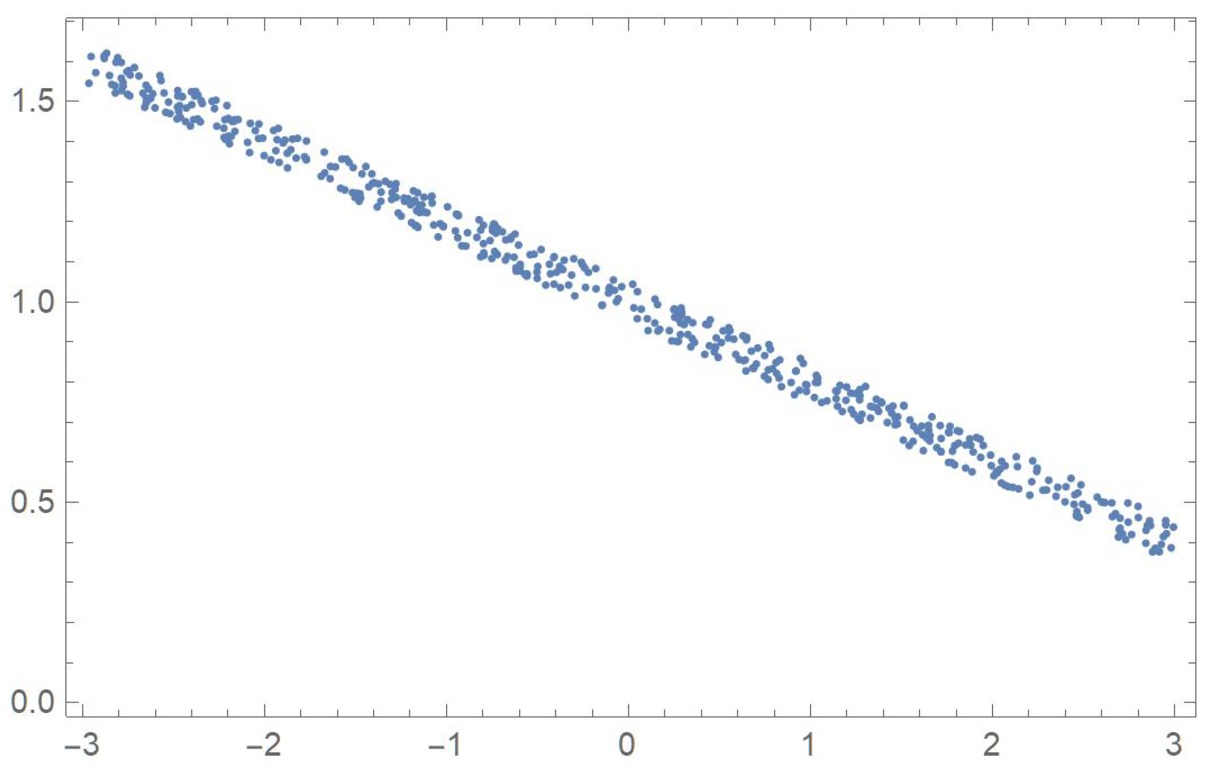
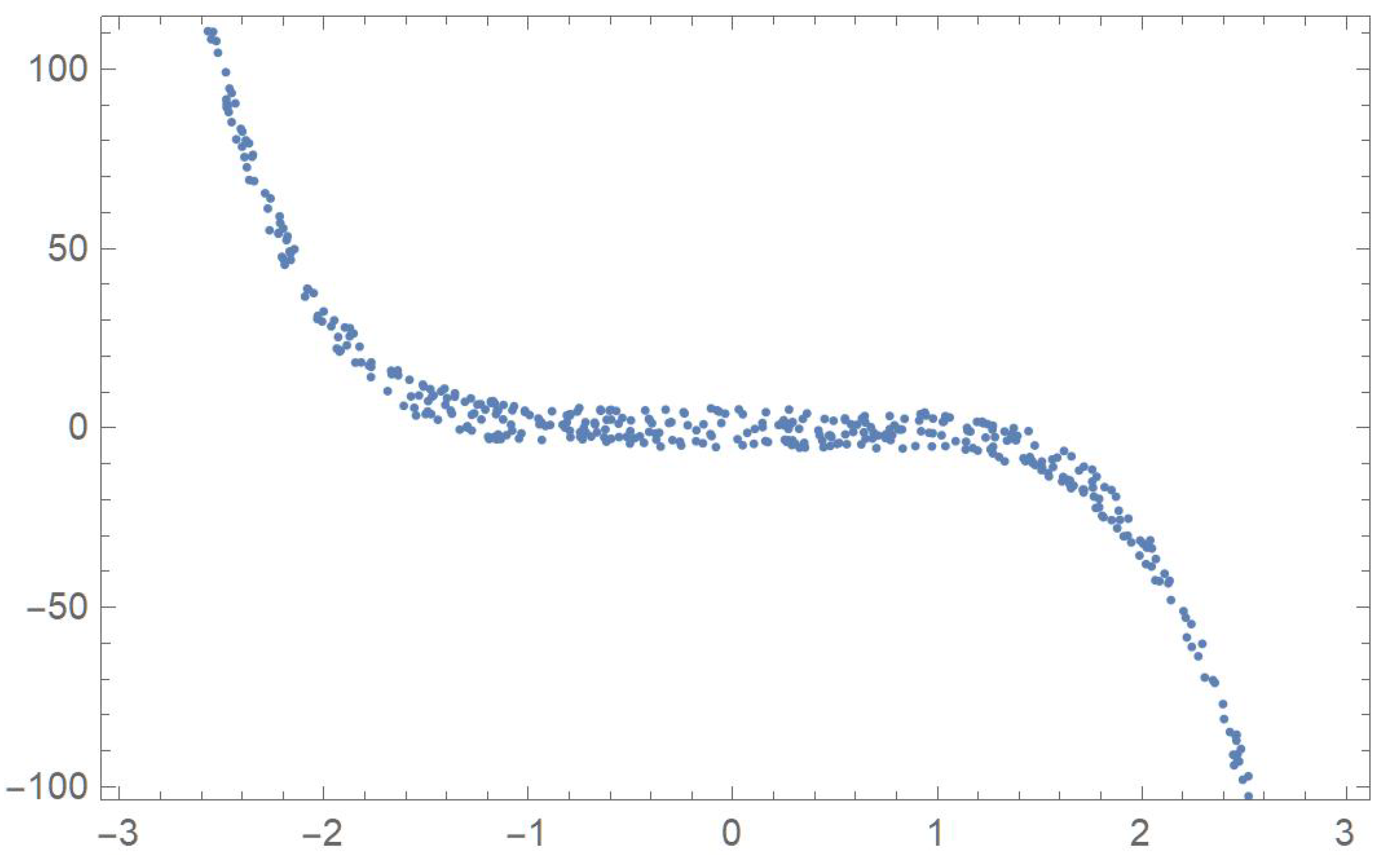
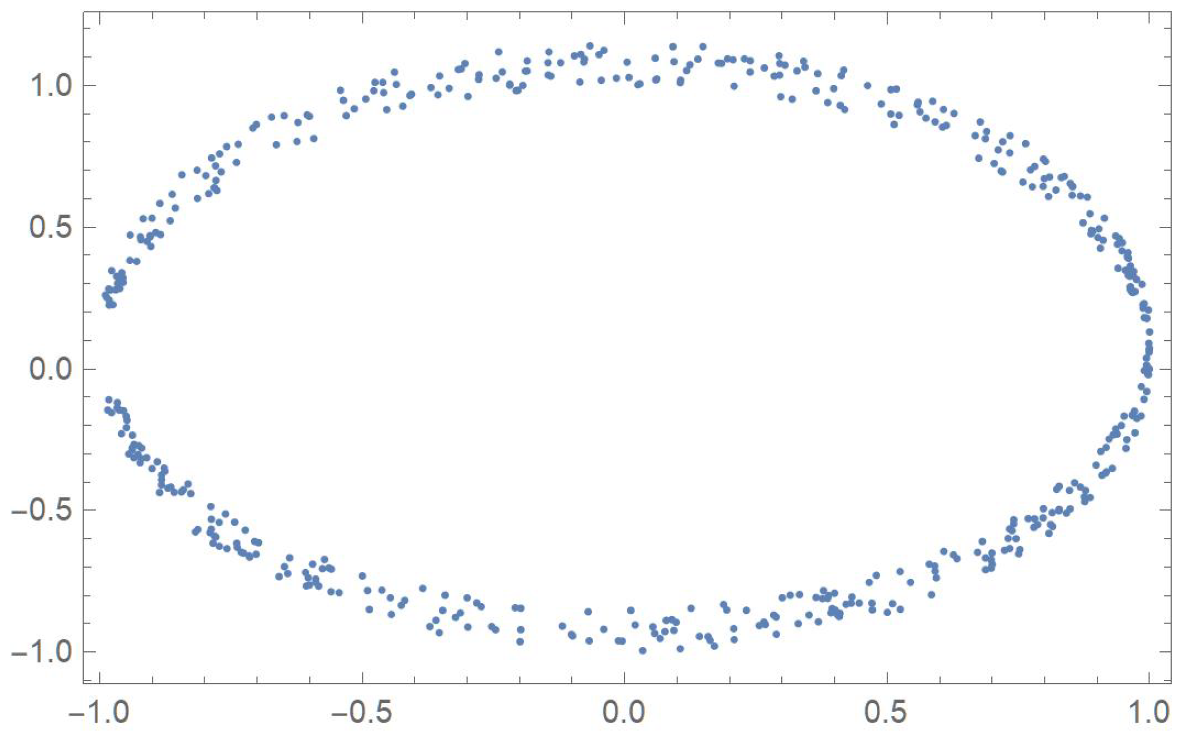
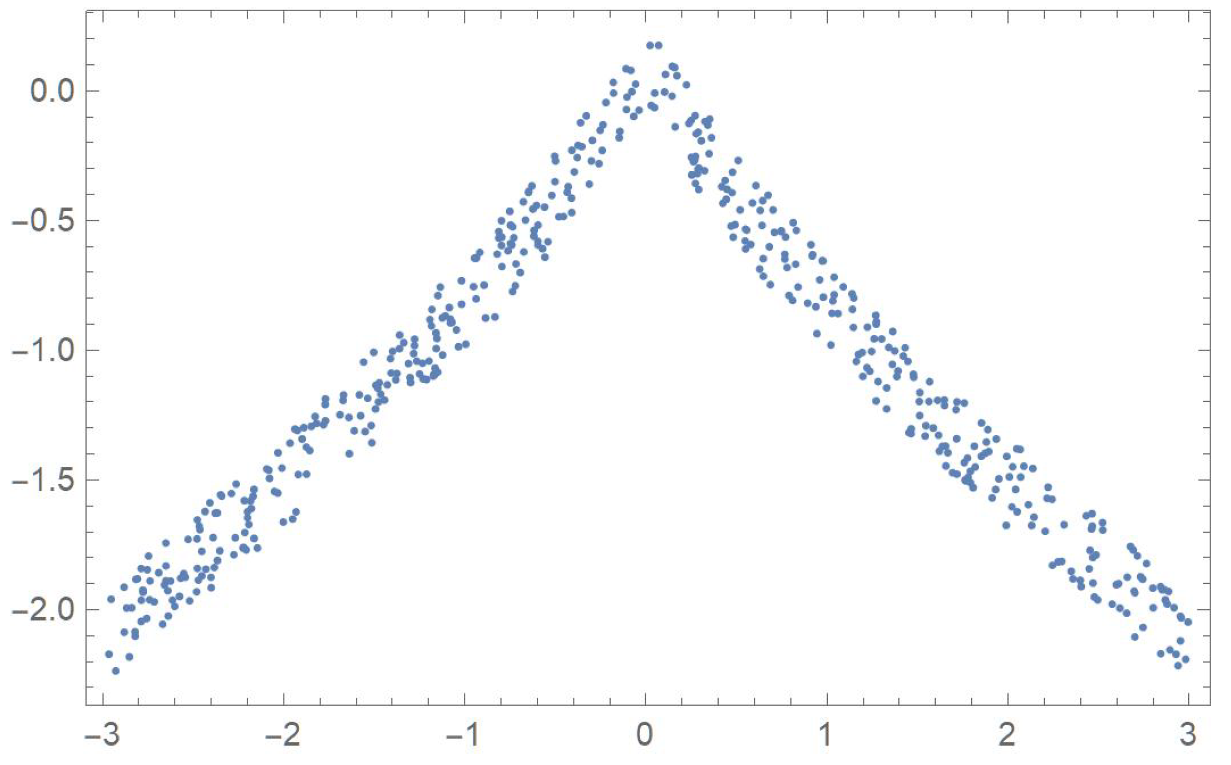
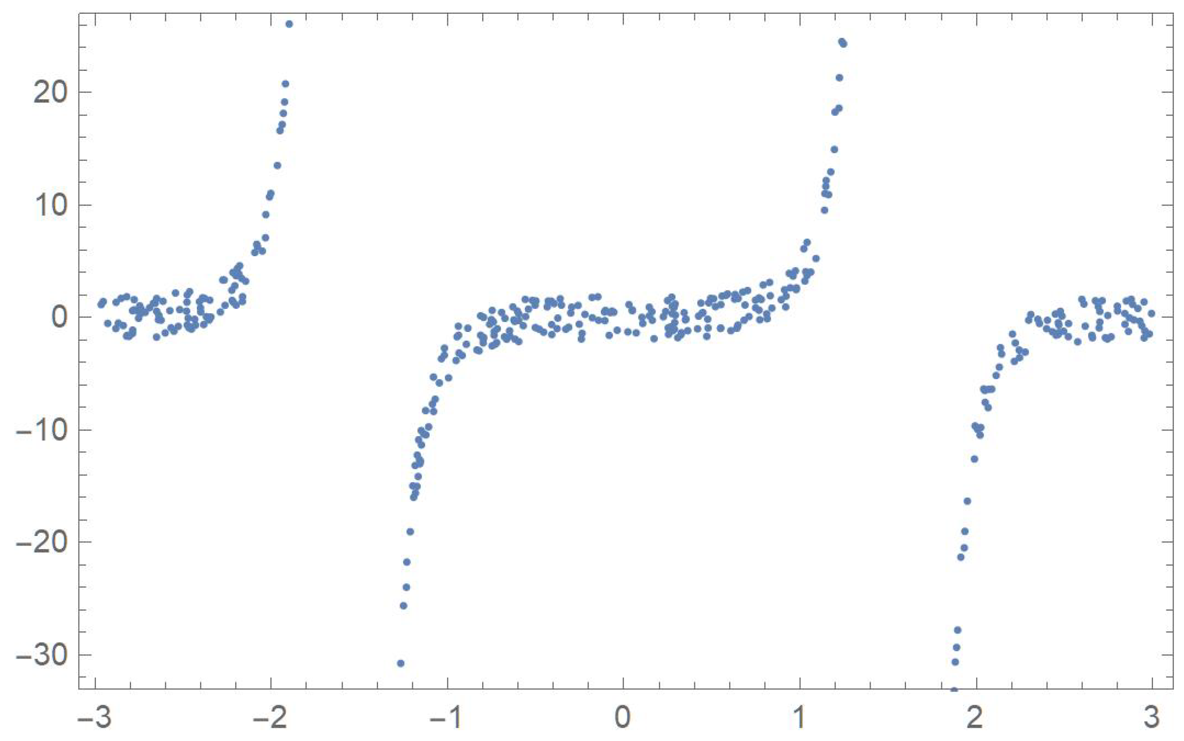
In order to compare the measures of association discussed in the previous sections, five two-dimensional data sets exhibiting different patterns that will be identified by the letters A, B, C, D and E, are considered. The first one was linearly decreasing, in which case Pearson’s correlation ought to be the most appropriate coefficient. The strictly monotonic pattern of the second set ought to be readily detected by Spearman’s, Kendall’s and Blomqvist’s coefficients, whose performance is assessed when applied to the fourth pattern, which happens to be piecewise monotonic. In the case of patterns C and E, whose points exhibit distinctive patterns, Hoeffding’s measure of dependence is expected to be more suitable than any of the other measures of association.

First, 500 random values of x, denoted by $\mathcal{S}$, were generated within the interval $(-3,3)$. Now, let

• $f_A\left(x\right)=-x/5+1+ϵ$,
• $f_B\left(x\right)=-x^5+ϵ$,
• $f_C\left(x\right)=\sin \left(x\right)+ϵ$,
• $f_D\left(x\right)=-\sqrt{|x^{3/2}|}+ϵ$ and
• $f_E=\tan {\left(x\right)}^3+ϵ,$

where $ϵ$ represents a slight perturbation consisting of a multiple of random values generated from a uniform distribution on the interval $[-1,1]$. The five resulting data sets, $A=\left\{(x,f_A\left(x\right))\right|x\in \mathcal{S}\}$, $B=\left\{(x,f_B\left(x\right))\right|x\in \mathcal{S}\}$, $C=\left\{(\cos \left(x\right),f_C\left(x\right))\right|x\in \mathcal{S}\}$, $D=\left\{(x,f_D\left(x\right))\right|x\in \mathcal{S}\}$ and $E=\left\{(x,f_E\left(x\right))\right|x\in \mathcal{S}\}$ are plotted in Figure 1, Figure 2, Figure 3, Figure 4 and Figure 5.

We then evaluated Spearman’s, Kendall’s, Blomqvist’s and Hoeffding’s statistics, as well as Pearson’s sample correlation coefficient for each data set. Their numerical values and associated p-values are reported in

Table 1. Five statistics and their associated p-values.

Statistics and p-Values	A	B	C	D	E
Spearman	{$-0.9963,0$}	{$-0.9218,0$}	{0.0022, 0.9602}	{0.1028, 0.0215}	{$-0.0745,0.0961$}
Kendall	{$-0.9456,0$}	{$-0.8072,0$}	{0.0071, 0.8136}	{0.0919, 0.0021}	{$-0.0350,0.2419$}
Blomqvist	{$-0.9600,0$}	{$-0.6160,0$}	{0.0320, 0.4209}	{0.0720, 0.0891}	{0.0640, 0.1283}
Hoeffding	{0.8679, 0}	{0.5302, 0}	{0.0472, 0}	{0.1902, 0}	{0.0104, 0}
Pearson	{$-0.9964,0$}	{$-0.8207,0$}	{0.0202, 0.6529}	{0.0555, 0.2152}	{$-0.0092,0.8377$}

.

Hoeffding’s statistic strongly rejects the null hypothesis of independence since the p-values are all virtually equal to zero. This correctly indicates that, in all five cases, the variables are functionally related.

As anticipated, Pearson’s correlation coefficient is larger in absolute value in the case of a linear relationship (data set A) with a value of $-0.9964,$ than in the case of a monotonic relationship (data set B) with a value of $-0.8207$.

Spearman’s, Kendall’s and Blomqvist’s statistics readily detect the monotonic relationships that data sets A and B exhibit. Interestingly, in the case of data set D, which happens to be monotonically increasing and then decreasing, at the 5% significance level, both Spearman’s and Kendall’s statistics manage to reject the independence assumption.

7. Multivariate Measures of Association

7.1. Blomqvist’s β

Consider the random vector $(X_1,X_2,\dots ,X_n)$ whose joint distribution function is $F\left(\mathbf{x}\right)=P(X_1\le x_1,X_2\le x_2,\dots ,X_n\le x_n)$ and marginal continuous distribution functions are $F_i\left(x_i\right)=P(X_i\le x_i)$ for $x_i\in \mathbb{R}$, $i\in \{1,2,\dots ,n\}$. We now state Sklar’s Theorem for the multivariate case:

Let F be an n-dimensional continuous distribution function with continuous marginal distribution functions ${(F}_1,F_2,\dots ,F_n)$. Then, there exists a unique n-copula $C:{\mathbb{1}}^n\to \mathbb{1}$ such that

$$F(x_1,x_2,\dots ,x_n)=C(F_1\left(x_1\right),F_2\left(x_2\right),\dots ,F_n\left(x_n\right)).$$

(69)

Conversely, if C is an n-copula and $F_1,F_2,\dots ,F_n$ are continuous distribution functions, then the function F is an n-dimensional distribution function with marginal distribution functions $(F_1,F_2,\dots ,F_n)$ [5] (Theorem 2.10.9, p. 46).

Clearly, the copula $C(·)$ in Equation (69) is the joint distribution function of the random variables $U_i=F_i\left(x_i\right)$, $i\in \{1,2,\dots ,n\}$. Observe that $C\left(\mathbf{u}\right)=P(\mathbf{U}\le \mathbf{u})=F(F_1^{-1}\left(u_1\right),F_2^{-1}\left(u_2\right),\dots ,F_n^{-1}\left(u_n\right))$ for all $\mathbf{u}=(u_1,\dots ,u_n)\in {\mathbb{1}}^n$.

Letting $W^n\left(\mathbf{u}\right)=\max (u_1+u_2+\cdots +u_n-n+1,0)$ and $M^n\left(\mathbf{u}\right)=\min (u_1,u_2,\dots ,u_n)$, the Fréchet–Hoeffding inequality,

$$W^n\left(\mathbf{u}\right)\le C\left(\mathbf{u}\right)\le M^n\left(\mathbf{u}\right),$$

(70)

provides lower and upper bounds for any copula. This inequality is attributed to [26,35]. We note that a related result appeared in [36].

The Fréchet–Hoeffding upper bound is a copula when the random variables are perfectly positively dependent, i.e., they are comonotonic. However, the lower bound is a copula only in the bivariate case [8].

Blomqvist’s $\beta$, as given in Equation (52), can also be expressed as

$$\beta =\frac{C(1/2,1/2)-\Pi (1/2,1/2)+\overline{C}(1/2,1/2)-\overline{\Pi }(1/2,1/2)}{M(1/2,1/2)-\Pi (1/2,1/2)+\overline{M}(1/2,1/2)-\overline{\Pi }(1/2,1/2)}.$$

(71)

where ${\Pi }^n\left(\mathbf{u}\right)=u_1{u}_2\cdots u_n$, and the survival function $\overline{C}\left(\mathbf{u}\right)=P(\mathbf{U}>\mathbf{u})$. When C is a copula involving n random variables, Equation (71) can be generalized as follows:

$$\begin{array}{cc}\hfill \beta & =\frac{C(\mathbf{1}/\mathbf{2})-\Pi (\mathbf{1}/\mathbf{2})+\overline{C}(\mathbf{1}/\mathbf{2})-\overline{\Pi }(\mathbf{1}/\mathbf{2})}{M(\mathbf{1}/\mathbf{2})-\Pi (\mathbf{1}/\mathbf{2})+\overline{M}(\mathbf{1}/\mathbf{2})-\overline{\Pi }(\mathbf{1}/\mathbf{2})}\hfill \\ \hfill & =k_n(C(\mathbf{1}/\mathbf{2})+\overline{C}(\mathbf{1}/\mathbf{2})-2^{1-n}),\hfill \end{array}$$

(72)

where $\mathbf{1}/\mathbf{2}=(1/2,1/2,\dots ,1/2)$, $k_n=\frac{2^{n-1}}{2^{n-1}-1}$, $\Pi (\mathbf{1}/\mathbf{2})=2^{-n}$, and $M(\mathbf{1}/\mathbf{2})=1/2$. When $n=2$, one has $C(1/2,1/2)=\overline{C}(1/2,1/2)$ for any copula; however, this is not the case for $n\ge 3$. The coefficient $\beta$ can be interpreted as the normalized average distance between the copula C and the independence copula $\Pi$.

Ref. [37] utilized the multivariate Blomqvist measure of dependence to analyze main GDP (gross domestic product) aggregates per capita in the European Union, Germany and Portugal for the period 2008–2019.

7.2. Spearman’s ρ

In the bivariate case, Spearman’s rank correlation can be expressed as

$${\rho }_S=\frac{E\left(UV\right)-E\left(U\right)E\left(V\right)}{\sqrt{\mathrm{Var}\left(U\right)\mathrm{Var}\left(V\right)}},$$

(73)

where U and V are uniformly distributed, so that $E\left(U\right)=E\left(V\right)=1/2$ and $\mathrm{Var}\left(U\right)=\mathrm{Var}\left(V\right)=1/12$. As previously established,

$$\begin{array}{cc}\hfill {\rho }_S& =\frac{{\int }_0^1{\int }_0^{1}uv\mathrm{d}C(u,v)-{(1/2)}^2}{1/12}\hfill \\ \hfill & =12{\int }_0^1{\int }_0^{1}C(u,v)\mathrm{d}u\mathrm{d}v-3,\hfill \end{array}$$

(74)

where C is the joint distribution of $(U,V)$.

Employing the same notation as in the previous section, we now present different versions of Spearman’s $\rho$ for the multivariate case:

(i)

Kendall (1970) [38]:

$${\rho }_{S4}=h_2(4\sum _{i<j}{\left(C_2^n\right)}^{-1}{\int }_{{[0,1]}^n}{C}_{ij}(u,v)\mathrm{d}u\mathrm{d}v-1);$$

(75)

(ii)

Ruymgaart and van Zuijlen (1978) [39]:

$${\rho }_{S1}=h_n(2^n{\int }_{{[0,1]}^n}C\left(\mathbf{u}\right)\mathrm{d}\mathbf{u}-1);$$

(76)

(iii)

Joe (1990) [40]:

$${\rho }_{S2}=h_n(2^n{\int }_{{[0,1]}^n}\mathbf{\Pi }\left(\mathbf{u}\right)\mathrm{d}C\left(\mathbf{u}\right)-1);$$

(77)

(iv)

Nelsen (2002) [2]:

$${\rho }_{S3}=h_n\left\{2^{n-1}({\int }_{{[0,1]}^n}C\left(\mathbf{u}\right)\mathrm{d}\mathbf{\Pi }\left(\mathbf{u}\right)+{\int }_{{[0,1]}^n}\mathbf{\Pi }\left(\mathbf{u}\right)\mathrm{d}C\left(\mathbf{u}\right)-1)\right\};$$

(78)

where $h_n=\frac{1+n}{2^n-(1+n)}$, $C_2^n=\frac{n!}{2!(n-2)!}$, and $\mathbf{u}=(u_1,u_2,\dots ,u_n)$.

We observe that ${\rho }_{S3}$ appears in [41] (p. 227) as a measure of average upper and lower orthant dependence, and that ${\rho }_{S4}$ constitutes the population version of the weighted average pairwise Spearman’s rho given in Chapter 6 of [38], where $C_{ij}(u,v)$ is the bivariate marginal copula [6] (p. 22).

As obtained by [41] (p. 228), a lower bound for ${\rho }_{Si},i\in \{1,2,3\}$, is given by

$$\frac{2^n-(n+1)!}{n!\{2^n-(n+1)\}}\mathrm{for}n\ge 2.$$

For $n=3$, this lower bound is at least equal to $-4/3$, and for $n=2$, we have ${\rho }_{S1}={\rho }_{S2}={\rho }_{S4}$. As noted by [42] (p. 787), the aforementioned lower bound may fail to be the best possible.

Spearman’s rank correlation can also be expressed as follows for the bivariate case:

$$\begin{array}{cc}\hfill {\rho }_S& =\frac{{\int }_{{[0,1]}^2}C(u,v)\mathrm{d}u\mathrm{d}v-{\int }_{{[0,1]}^2}\Pi (u,v)\mathrm{d}u\mathrm{d}v}{{\int }_{{[0,1]}^2}M(u,v)\mathrm{d}u\mathrm{d}v-{\int }_{{[0,1]}^2}\Pi (u,v)\mathrm{d}u\mathrm{d}v}\hfill \end{array}$$

(79)

$$\begin{array}{cc}\hfill & =\frac{{\int }_{{[0,1]}^2}uv\mathrm{d}C(u,v)-{\int }_{{[0,1]}^2}uv\mathrm{d}\Pi (u,v)}{{\int }_{{[0,1]}^2}uv\mathrm{d}M(u,v)-{\int }_{{[0,1]}^2}uv\mathrm{d}\Pi (u,v)},\hfill \end{array}$$

(80)

where ${\int }_{{[0,1]}^2}M(u,v)\mathrm{d}u\mathrm{d}v=1/3$ and ${\int }_{{[0,1]}^2}\Pi (u,v)\mathrm{d}u\mathrm{d}v=1/4$. It is readily seen that representation (79) coincides with that given in (74). The coefficient ${\rho }_S$ can be interpreted as the normalized average distance between the copula C and the independence copula $\Pi$.

Equation (79) suggests the following natural generalization for the multivariate case:

$${\rho }_S=\frac{{\int }_{{[0,1]}^n}C\left(\mathbf{u}\right)\mathrm{d}\mathbf{u}-{\int }_{{[0,1]}^n}\Pi \left(\mathbf{u}\right)\mathrm{d}\mathbf{u}}{{\int }_{{[0,1]}^n}M\left(\mathbf{u}\right)\mathrm{d}\mathbf{u}-{\int }_{{[0,1]}^n}\Pi \left(\mathbf{u}\right)\mathrm{d}\mathbf{u}},$$

(81)

which, incidentally, agrees with the representation specified in Equation (76).

For instance, Liebscher (2021) [43] made use of the multivariate Spearman measure of correlation to determine the dependence of a response variable on a set of regressor variables in a nonparametric regression model.

7.3. Kendall’s τ

Joe (1990) [40] provides the following representation of Kendall’s $\tau$ for the multivariate case:

$${\tau }_{n,c}={(2^{n-1}-1)}^{-1}\{2^n{\int }_{{[0,1]}^n}C\left(\mathbf{u}\right)\mathrm{d}C\left(\mathbf{u}\right)-1\},$$

(82)

which also appears in [5] (p. 231) as measure of average multivariate total positivity. In fact, Equation (82) generalizes Equation (44), i.e.,

$${\tau }_{2,c}=4{\int }_0^1{\int }_0^{1}C(u_1,u_2)\mathrm{d}C(u_1,u_2)-1.$$

(83)

Nelsen (1996) [41] also notes that a lower bound for ${\tau }_{n,c}$ is given by

$$-{(2^{n-1}-1)}^{-1}\sin \mathrm{ce}{\int }_{{[0,1]}^n}C\left(\mathbf{u}\right)\mathrm{d}C\left(\mathbf{u}\right)\ge 0.$$

(84)

As shown by [42] (Theorem 5.1), and reported by [44] (p. 218), this lower bound is attained if at least one of the bivariate margins of the copula C equals W (the Fréchet–Hoeffding lower bound).

Kendall and Babington Smith (1940) [45] introduced an extension of Kendall’s $\tau$ as a coefficient of agreement among $n\ge 2$ rankings. Another generalization is proposed in [46].

A test based on the nonparametric estimator of the multivariate extension of Kendall’s $\tau$ was utilized in [47] to establish links between innovation and higher education in certain regions.

7.4. Hoeffding’s Φ²

Using the same notation as in the previous sections, one can express Hoeffding’s dependence index as follows for the bivariate case:

$$\begin{array}{cc}\hfill {\mathsf{\Phi }}_{X,Y}^2& =90{\int }_0^1{\int }_0^1{\{C(u,v)-uv\}}^2\mathrm{d}u\mathrm{d}v\hfill \\ \hfill & =90{\int }_{{[0,1]}^2}{\{C(u,v)-\Pi (u,v)\}}^2\mathrm{d}u\mathrm{d}v,\hfill \end{array}$$

(85)

where

$${\mathsf{\Phi }}_{X,Y}^2=\left\{\begin{array}{cc}0\hfill & \mathrm{in}\mathrm{the}\mathrm{case}\mathrm{of}\mathrm{stochastic}\mathrm{independence},\hfill \\ 1\hfill & \mathrm{in}\mathrm{the}\mathrm{case}\mathrm{of}\mathrm{monotone}\mathrm{dependence},\hfill \\ (0,1),\hfill & \mathrm{otherwise}.\hfill \end{array}\right.$$

(86)

Observe that ${\mathsf{\Phi }}_{X,Y}^2=0$ if and only if $C=\Pi$.

For the multivariate case, ${\mathsf{\Phi }}^2$ is defined as

$${\mathsf{\Phi }}^2=h_n{\int }_{{[0,1]}^n}{\{C\left(\mathbf{u}\right)-\Pi \left(\mathbf{u}\right)\}}^2\mathrm{d}\mathbf{u},$$

(87)

where $h_n={\left[{\int }_{{[0,1]}^n}{\{M\left(\mathbf{u}\right)\mathrm{d}\mathbf{u}-\Pi \left(\mathbf{u}\right)\mathrm{d}\mathbf{u}\}}^2\right]}^{-1}$ is the normalizing constant.

Gaißer et al. (2010) [30] determined that the inverses of the normalizing constants for the upper and lower bounds are, respectively, given by

$$\begin{array}{cc}\hfill {\left(h_n\right)}^{-1}& ={\int }_{{[0,1]}^n}{\{M\left(\mathbf{u}\right)\mathrm{d}\mathbf{u}-\Pi \left(\mathbf{u}\right)\}}^2\mathrm{d}\mathbf{u}\hfill \\ \hfill & =\frac{2}{(n+1)(n+2)}-\frac{2^{-n}n!}{{\prod }_{i=0}^n(i+1/2)}+{(1/3)}^n\hfill \end{array}$$

(88)

and

$$\begin{array}{cc}\hfill {\left(g_n\right)}^{-1}& ={\int }_{{[0,1]}^n}{\{W\left(\mathbf{u}\right)\mathrm{d}\mathbf{u}-\Pi \left(\mathbf{u}\right)\}}^2\mathrm{d}\mathbf{u}\hfill \\ \hfill & =\frac{2}{(n+2)!}-2\sum _{i=0}^n{C}_i^n{(-1)}^i\frac{1}{(n+1+i)!}+{(1/3)}^n,\hfill \end{array}$$

(89)

where $C_i^n=\frac{n!}{i!(n-i)!}$.

For instance, Medovikov and Prokhorov (2017) [48] made use of Hoeffding’s multivariate index to determine the dependence structure of financial assets and evaluate the risk of contagion.

7.5. Note

As pointed out by [49], Spearman’s $\rho$ and Blomqvist’s $\beta$ can be expressed as follows:

$$k_n\left(C\right)={\alpha }_n\left\{{\int }_{{[0,1]}^n}(C+{\sigma }^{*})\mathrm{d}{\mu }_n-\frac{1}{2^{n-1}}\right\},$$

(90)

where ${\mu }_n$ is a probability measure on ${[0,1]}^n$, whereas Kendall’s $\tau$ has the following representation:

$${\tau }_n\left(C\right)={\alpha }_n\left\{{\int }_{{[0,1]}^n}C\mathrm{d}C-\frac{1}{2^n}\right\},$$

(91)

with

$$\begin{array}{cc}\hfill {\alpha }_n& =\frac{(1+n)2^{n-1}}{2^n-(1+n)},\mathrm{for}\mathrm{Spearman}’\mathrm{s}\mathrm{rho},\hfill \\ \hfill {\alpha }_n& =\frac{2^{n-1}}{2^{n-1}-1},\mathrm{for}\mathrm{Blomqvist}’\mathrm{s}\mathrm{beta},\hfill \end{array}$$

and

$$\begin{array}{cc}\hfill {\alpha }_n& =\frac{2^n}{2^{n-1}-1},\mathrm{for}\mathrm{Kendall}’\mathrm{s}\mathrm{tau}.\hfill \end{array}$$

8. Conclusions

Bivariate and multivariate measures of dependence originally due to Spearman, Kendall, Blomqvist and Hoeffding, as well as related results of interest such as their sample estimators and representations in terms of copulas, were discussed in this paper. Various recent applications were also pointed out. Additionally, a numerical study corroborated the effectiveness of these coefficients of association in assessing dependence with respect to five sets of generated data exhibiting various patterns.

A potential avenue for future research would consist in studying matrix-variate rank correlation measures as was achieved very recently by [50] for the case of Kendall’s $\tau$.

References

- Sklar, A. Fonctions de répartition à n dimensions et leurs marges. Publ. l’Institut Stat. l’Université Paris 1959, 8, 229–231. [Google Scholar]
- Nelsen, R.B. Concordance and copulas: A survey. In Distributions with Given Marginals and Statistical Modelling; Cuadras, C.M., Fortiana, J., Rodriguez-Lallena, J.A., Eds.; Kluwer Academic Publishers: London, UK, 2002; pp. 169–177. [Google Scholar]
- Deheuvels, P. La fonction de dépendance empirique et ses propriétés, un test non-paramétrique d’indépendance. Bullettin l’Académie R. Belg. 1979, 65, 274–292. [Google Scholar] [CrossRef]
- Joe, H. Multivariate Models and Dependence Concepts; Chapman & Hall: Boca Raton, FL, USA, 1997. [Google Scholar]
- Nelsen, R.B. An Introduction to Copulas, 2nd ed.; Springer: New York, NY, USA, 2006. [Google Scholar]
- Cherubini, U.; Fabio, G.; Mulinacci, S.; Romagno, S. Dynamic Copula Methods in Finance; John Wiley & Sons: New York, NY, USA, 2012. [Google Scholar]
- Kojadinovic, I.; Yan, J. Comparison of three semiparametric methods for estimating dependence parameters in copula models. Math. Econ. 2010, 47, 52–63. [Google Scholar] [CrossRef]
- Schmid, F.; Schmidt, R. Nonparametric inference on multivariate versions of Blomqvist’s beta and related measures of tail dependence. Metrika 2007, 66, 323–354. [Google Scholar] [CrossRef]
- Genest, C.; Ghoudi, K.; Rivest, L.-P. A semiparametric estimation procedure of dependence parameters in multivariate families of distribution. Biometrika 1995, 82, 543–552. [Google Scholar] [CrossRef]
- Dias, A. Maximum pseudo-likelihood estimation in copula models for small weakly dependent samples. arXiv 2022, arXiv:2208.01322. [Google Scholar]
- Kerman, J. A closed-form approximation for the median of the beta distribution. arXiv 2011, arXiv:1111.0433. [Google Scholar]
- Schweizer, B.; Wolff, E.F. On nonparametric measures of dependence for random variables. Ann. Stat. 1981, 9, 879–885. [Google Scholar] [CrossRef]
- Rényi, A. On measures of dependence. Acta Math. Hung. 1959, 10, 441–451. [Google Scholar] [CrossRef]
- Lai, C.D.; Balakrishnan, N. Continuous Bivariate Distributions, 2nd ed.; Springer: New York, NY, USA, 2009. [Google Scholar]
- Gibbons, J.D.; Chakraborti, S. Nonparametric Statistical Inference, 4th ed.; Revised and Expanded; Statistics Textbooks and Monographs; Marcel Dekker, Inc.: New York, NY, USA, 2003; Volume 168. [Google Scholar]
- Hofert, M.; Kojadinovic, I.; Mächler, M.; Yan, J. Elements of Copula Modeling with R; Springer: New York, NY, USA, 2019. [Google Scholar]
- Kendall, M.G. A new measure of rank correlation. Biometrika 1938, 30, 81–93. [Google Scholar] [CrossRef]
- Kruskal, W.H. Ordinal measures of association. J. Am. Stat. Assoc. 1958, 53, 814–861. [Google Scholar] [CrossRef]
- Kendall, M.G.; Gibbons, J.D. Rank Correlation Methods, 5th ed.; Griffin: London, UK, 1990. [Google Scholar]
- Lipps, G.F. Die Betimmung der Abhängigkeit zwischen den Merkmalen eines Gegeständes. Berichte Königlich Säsischen Ges. Wiss. 1905, 57, 1–32. [Google Scholar]
- Lipps, G.F. Die Psychischen Massmethoden; (No. 10); F. Vieweg und Sohn: Braunschweig, Germany, 1906. [Google Scholar]
- Fechner, G.T. Kollektivmasslehre; Engelmann: Kogarah, Australia, 1897. [Google Scholar]
- Blomqvist, N. On a measure of dependence between two random variables. Ann. Math. Stat. 1950, 21, 593–600. [Google Scholar] [CrossRef]
- Genest, C.; Carabarín-Aguirre, A.; Harvey, F. Copula parameter estimation using Blomqvist’s beta. J. Société Française Stat. 2013, 154, 5–24. [Google Scholar]
- Mosteller, F. On some useful “inefficient” statistics. Ann. Math. Stat. 1946, 17, 377–408. [Google Scholar] [CrossRef]
- Hoeffding, W. Masstabinvariante Korrelationstheorie. Schriften Math. Instituts Instituts Angew. Math. Universität Berlin 2012, 5, 181–233. [Google Scholar]
- Lehmann, E.L. Some concepts of dependence. T Ann. Math. Stat. 1966, 37, 1137–1153. [Google Scholar] [CrossRef]
- Jogdeo, K. Characterizations of independence in certain families of bivariate and multivariate distributions. Ann. Math. Stat. 1968, 39, 433–441. [Google Scholar] [CrossRef]
- Block, H.W.; Fang, Z. A multivariate extension of Hoeffding’s lemma. Ann. Probab. 1988, 16, 1803–1820. [Google Scholar] [CrossRef]
- Gaißer, S.; Ruppert, M.; Schmid, F. A multivariate version of Hoeffding’s phi-square. J. Multivar. Anal. 2010, 101, 2571–2586. [Google Scholar] [CrossRef]
- Gänssler, P.; Stute, W. Seminar on Empirical Processes; DMV Seminar 9; Birkhäuser: Basel, Switzerland, 1987. [Google Scholar]
- Van der Vaart, A.W.; Wellner, J.A. Weak Convergence and Empirical Processes; Springer: New York, NY, USA, 1996. [Google Scholar]
- Tsukahara, H. Semiparametric estimation in copula models. Can. J. Stat. 2005, 33, 357–375. [Google Scholar] [CrossRef]
- Blum, J.R.; Kiefer, J.; Rosenblatt, M. Distribution free tests of independence based on the sample distribution function. Ann. Math. Stat. 1961, 32, 485–498. [Google Scholar] [CrossRef]
- Fréchet, M. Sur les tableaux de corrélations dont les marges sont données. Ann. L’Université Lyon 1951, 9, 53–77. [Google Scholar]
- Fréchet, M. Généralisations du théorème des probabilités totales. Fundam. Math. 1935, 25, 379–387. [Google Scholar] [CrossRef]
- Ferreira, H.; Ferreira, M. Multivariate medial correlation with applications. Depend. Model. 2020, 8, 361–372. [Google Scholar] [CrossRef]
- Kendall, M.G. Rank Correlation Methods; Griffin: London, UK, 1970. [Google Scholar]
- Ruymgaart, F.H.; van Zuijlen, M.C.A. Asymptotic Normality of Multivariate Linear Rank Statistics in the Non-I.I.D. Case. Ann. Stat. 1978, 6, 588–602. [Google Scholar] [CrossRef]
- Joe, H. Multivariate Concordance. J. Multivar. Anal. 1990, 35, 12–30. [Google Scholar] [CrossRef]
- Ne1sen, R.B. Nonparametric measures of multivariate association. In Distributions with Fixed Marginals and Related Topics; Rüschendorf, L., Schweizer, B., Taylor, M.D., Eds.; Institute of Mathematical Statistics: Hayward, CA, USA, 1996; pp. 223–232. [Google Scholar]
- Úbeda-Flores, M. Multivariate versions of Blomqvist’s Beta and Spearman’s footrule. Ann. Inst. Stat. Math. 2005, 57, 781–788. [Google Scholar] [CrossRef]
- Liebscher, E. On a multivariate version of Spearman’s correlation coefficient for regression: Properties and Applications. Asian J. Stat. Sci. 2021, 1, 123–150. [Google Scholar]
- Schmid, F.; Schmidt, R.; Blumentritt, T.; Gaißer, S.; Ruppert, M. Copula-Based Measures of Multivariate Association in Copula Theory and Its Applications. In Lecture Notes in Statistics; Jaworski, P., Durante, F., Härdle, W., Rychlik, T., Eds.; Springer: Berlin, Germany, 2010; Volume 198. [Google Scholar]
- Kendall, M.G.; Babington Smith, B. On the method of paired comparisons. Biometrika 1940, 31, 324–345. [Google Scholar] [CrossRef]
- Genest, C.; Nešlehová, J.; Ghorbal, N.B. Estimators based on Kendall’s tau in multivariate copula models. Aust. N. Z. J. Stat. 2011, 53, 157–177. [Google Scholar] [CrossRef]
- Ascorbebeitia, J.; Ferreira, E.; Orbe, S. Testing conditional multivariate rank correlations: The effect of institutional quality on factors influencing competitiveness. TEST 2022, 31, 931–949. [Google Scholar] [CrossRef]
- Medovikov, I.; Prokhorov, A. A new measure of vector dependence, with applications to financial risk and contagion. J. Financ. Econom. 2017, 15, 474–503. [Google Scholar] [CrossRef]
- Taylor, M.D. Multivariate measures of concordance for copulas and their marginals. Depend. Model. 2016, 4, 224–236. [Google Scholar] [CrossRef]
- McNeil, A.J.; Nešlehová, J.G.; Smith, A.D. On Attainability of Kendall’s Tau Matrices and Concordance Signatures. J. Multivar. Anal. 2022, 191, 105033. [Google Scholar] [CrossRef]
Figure 1.
Plot of data set A.
Figure 2.
Plot of data set B.
Figure 3.
Plot of data set C.
Figure 4.
Plot of data set D.
Figure 5.
Plot of data set E.