The Reliability Inference for Multicomponent Stress–Strength Model under the Burr X Distribution

Abstract

The reliability of the multicomponent stress–strength system was investigated under the two-parameter Burr X distribution model. Based on the structure of the system, the type II censored sample of strength and random sample of stress were obtained for the study. The maximum likelihood estimators were established by utilizing the type II censored Burr X distributed strength and complete random stress data sets collected from the multicomponent system. Two related approximate confidence intervals were achieved by utilizing the delta method under the asymptotic normal distribution theory and parametric bootstrap procedure. Meanwhile, point and confidence interval estimators based on alternative generalized pivotal quantities were derived. Furthermore, a likelihood ratio test to infer the equality of both scalar parameters is provided. Finally, a practical example is provided for illustration.

1. Introduction

Systems or units that are subject to the competition between strength and stress have been studied under the commonly called stress–strength model. The system survives if the imposed stress is less than the system strength. Therefore, the stress–strength model plays a substantial role in many aspects, such as lifetime study, engineering, and supply and demand applications.

Let X be the system strength and Y be the stress applied. Then, the stress–strength reliability (SSR) is labeled as $R=P(Y<X)$. Generally, X indicates the measurement of quality characteristics for the main subject and Y indicates the measurement of quality characteristics for the opposite subject in the system. Next, three cases are presented to illustrate the applications of a stress–strength system. In mechanical engineering, the strength measure X of a long horizontal part for a crane needs to exceed the stress of the loading weight Y from the lifted object of operation. The reliability $R=P(Y<X)$ is an essential quantity for assessing the quality of a crane. In the application of civil engineering, the tolerable bearing capacity of a suspension bridge is an important quality measure. The bearing capacity X from a pair of cables for the suspension bridge should exceed the total weight Y of the cars. In this application, a high reliability $R=P(Y<X)$ is essential for a suspension bridge design. In logistics applications, the supply capacity X can represent the strength and the demand Y can represent the stress. A high reliability $R=P(Y<X)$ indicates a reliable logistics system. In recent years, the stress–strength model has been broadly used in a variety of fields, such as economics, hydrology, reliability engineering, seismology, and survival analysis. The system reliability has also been studied by numerous researchers. Eryilmaz [1] developed formulae for R and the mean residual life at random time based on phase-type distributions, such as the Erlang distribution. Kundu and Raqad [2] investigated a modified maximum likelihood estimation for R based on Weibull distributions, each of which possess three parameters: shape, scale, and location. Krishnamoorthy and Lin [3] studied confidence limits for R by using the generalized variable approach through the maximum likelihood estimation method with two independent Weibull distributions. Mokhlis et al. [4] investigated the inferences of R under distributions that include general exponential and inverse-exponential forms. Surles and Padgett [5] studied the maximum likelihood estimate and Bayesian inference for R based on Burr X distributions with the equal scale parameter set to one. Wang et al. [6] acquired inference procedures for R with a generalized exponential distribution.

Very often, like in the aforementioned references, the studies of reliability inference are mainly concentrated on a system with a main component. Nevertheless, several practical systems, such as a system with series components, parallel components, or any combination of these two, are composed of multiple components to accomplish the required functions. Therefore, multicomponent system reliability investigations have attracted more attention lately. Commonly, multicomponent systems consist of $k>1$ main components, of which the strengths follow an independent and identical distribution (i.i.d.) subject to an opposite commonly distributed stress. The system survives if at least $s(1\le s\le k)$ main components concurrently function. The multicomponent system is generally referred to as the s-out-of-k G system. There are numerous practical multicomponent systems in the world. For example, a communication system with three transmitters, where the expected message load requires at least two transmitters to be operational; otherwise, critical messages are lost. Hence, this transmission system is called a two-out-of-three G system. A second example, where the Airbus A-380 with four engines is capable of flying if and only if at least two of the four engines are functioning, is referred to as a two-out-of-four G system. Another example is a suspension bridge with k pairs of cables, which needs at least s pairs of unbroken cables to withstand the stress.

Let the k components’ strength variables in an s-out-of-k G system, where each component is subject to a stress measure Y, be $X_1,X_2,\dots ,X_k$. The multicomponent stress–strength reliability (MSR) $R_{s,k}$, as presented by Bhattacharyya and Johnson [7], is given by

$$\begin{array}{cc}\hfill R_{s,k}& =P\left(\mathrm{at}\mathrm{least}s\mathrm{of}\mathrm{the}(X_1,X_2,\dots ,X_k)\mathrm{exceed}Y\right)\hfill \\ \hfill & =\sum _{i=s}^k\left(\begin{array}{c}k\\ i\end{array}\right){\int }_{-\infty }^{\infty }{[1-F\left(w\right)]}^i{\left[F\left(w\right)\right]}^{k-i}dG\left(w\right),\hfill \end{array}$$

(1)

where $F(·)$ is the common cumulative distribution (CDF) of $X_1,X_2,\dots ,X_k$ and $G(·)$ is the CDF of Y. The reliability $R_{s,k}$ inferences for s-out-of-k G systems based on different distribution models have been extensively investigated by several researchers. The work by Dey et al. [8] was based on random samples from Kumaraswamy distributions. The work by Kayal et al. [9] was based on random samples from Chen distributions. The works by Kizilaslan [10,11] were based on random samples from proportional reversed hazard rate distributions and a general class of inverse exponentiated distributions, respectively. The work by Kizilaslan and Nadar [12] was based on complete sample sets from bivariate Kumaraswamy distributions. The work by Nadar and Kizilaslan [13] was based on complete samples from Marshall–Olkin bivariate Weibull distributions. The works by Rao [14,15] were, respectively, based on complete random samples from Rayleigh and generalized Rayleigh distributions. The work by Rao et al. [16] was based on complete random samples from Burr XII distributions. The work by Shawky and Khan [17] was based on random samples from inverse Weibull distributions. The work by Lio et al. [18] was based on type II sample of strength and complete random sample of stress Burr XII distributions. The work by Sauer et al. [19] was based on progressively type II censored samples from generalized Pareto distributions. And the work by Wang et al. [20] was based on type II censored strength and complete stress samples from Rayleigh stress–strength models.

Burr [21] developed numerous distributions. Among them, both Burr X and Burr XII have been the most attractive in recent reliability studies. Meanwhile, Belili et al. [22] explored an elastic two-parameter family of distributions and provided numerous theoretical results that include vital parameters and behaviors of distribution functions, reliability measurements for the proposed two-parameter family, and applications to annual maximum floods and survival times for breast cancer patients. The proposed two-parameter family of distributions include the two-parameter Lindley distributions I and II, gamma Lindley distribution, quasi-Lindley distributions, pseudo-Lindley distribution, and XLindley distribution as special cases, but do not include the Burr types. Their proposed family of distributions could potentially be applied to the stress–strength reliability inference for the multicomponent system. Yousof et al. [23] and Jamal and Nasir [24] proposed two Burr X generators to create different families of distributions by using the CDF of a one-parameter Burr X distribution composite with $-\ln \left(\overline{G}(t;\eta )\right)$ and $\frac{G(t;\eta )}{\overline{G}(t;\eta )}$, where $G(t;\eta )$ and $\overline{G}(t;\eta )$ are the CDF and survival function of a second distribution with parameter vector $\eta$ of one dimension or two dimensions, respectively. Therefore, both Burr X generalized distributions have two parameters or three parameters. Both papers developed numerous properties of these two generalized Burr X distributions that include stress–strength reliability for a one-component system. However, the practical application of stress–strength reliability was not provided. They also applied these two generalized Burr X distributions to model a random sample of 128 bladder cancer patients’ remission times (in months) and concurrently concluded that their respective extended Burr X distributions performed better than a one-parameter Burr X distribution. These two generalized Burr X distributions do not contain the current two-parameter Burr X distribution as a special case and could potentially be applied to the stress–strength reliability inference for a multicomponent system as well.

The Burr XII distribution has two shape parameters. For more information about Burr XII, readers may refer to Lio et al. [18]. The Burr X distribution considered in the current study has two parameters and the probability density function (PDF) and CDF, respectively, are defined as

$$\begin{array}{cc}\hfill & f(x;\lambda ,\alpha )=\frac{2x\alpha }{\lambda }exp(-x^2/\lambda ){(1-exp(-x^2/\lambda ))}^{(\alpha -1)}\mathrm{and}\hfill \\ \hfill & F(x;\lambda ,\alpha )={(1-exp(-x^2/\lambda ))}^{\alpha },x>0,\lambda >0,\alpha >0,\hfill \end{array}$$

(2)

where $\lambda$ and $\alpha$ are the scale and shape parameters, respectively. For easy reference, BurrX$(\lambda ,\alpha )$ is used as the Burr X distribution with parameters $\lambda$ and $\alpha$, hereafter. Because of the flexibility of use for any two-parameter distribution, BurrX$(\lambda ,\alpha )$ has been investigated in the reliability studies of numerous scholars. Jaheen [25] explored the reliability and failure rate functions for the Burr X model by utilizing the empirical Bayesian estimation method based on complete random samples. Ahmad et al. [26] considered the empirical Bayes estimate of R based on random samples from a Burr X distribution. When both stress and strength Burr X distributions have scale parameters of one, Surles and Padgett [5] and Akgul and Senoglu [27] studied the inference of R using maximum likelihood and Bayes methods based on random samples and using a modified maximum likelihood estimate method based on ranked set samples, respectively. Surles and Padgett [5] applied a Burr X distribution to model the stress and strength reliability of a one-component system based on the strengths of two carbon fibers. However, according to a literature search, work that investigated $R_{s,k}$ based on a Burr X distribution has not appeared.

In reality, we do not always obtain a complete random sample, except for censored data. Moreover, under the current multicomponent model, usually only type II strength sample and complete random stress observations can be observed from the system. Therefore, the current research focused on some alternative inferential methodologies for $R_{s,k}$ when the strength data are a type II censored Burr X distributed sample and the stress data are a Burr X distributed random sample. The estimation methods for $\lambda$, $\alpha$, and $R_{s,k}$ include maximum likelihood and pivotal quantity estimation methods for type II censored strength and random stress samples. Based on our best knowledge, the approaches used in this work have not appeared in the literature regarding BurrX$(\lambda ,\alpha )$.

Section 2 briefly describes the structure information about typical type II censored strength and associated stress data sets from the aforementioned G system and the likelihood function based on those data sets from n G systems. In Section 3, the maximum-likelihood-based approaches are addressed for Burr X distributions. Additionally, asymptotic confidence intervals (ACIs) are derived via utilizing the delta method and bootstrap percentile procedure. Inferences based on pivotal quantities are given in Section 4, where numerous theorems to support the existence and uniqueness of each pivotal-quantity-based estimator are established. For the model test of the equivalence of Burr X scale parameters for strength and stress, Section 5 provides a ratio test. Section 6 provides a real data example for demonstration. Some concluding remarks are given in Section 7.

2. The Likelihood Function Based on Sample from G System

In a lifetime-testing experiment using n s-out-of-k G systems, where each system contains k strength components subject to a common stress, the strength and stress samples can be obtained, respectively, as

$$\begin{array}{c}\hfill \begin{array}{ccc}\mathrm{Observed}\mathrm{strength}\mathrm{sample}& & \mathrm{Observed}\mathrm{stress}\mathrm{sample}\\ \left(\begin{array}{cccc}{X}_{11}& X_{12}& \cdots & X_{1s}\\ ⋮& ⋮& \ddots & ⋮\\ X_{n1}& X_{n2}& \cdots & X_{ns}\end{array}\right)& \mathrm{and}& \left(\begin{array}{c}{Y}_1\\ ⋮\\ Y_n\end{array}\right),\end{array}\end{array}$$

(3)

where $\{X_{i1}\le X_{i2}\le \dots \le X_{is}\}$ represents the first s ordered strength statistics under type II censoring and $Y_i$ represents the stress variable accordingly for $i=1,2,\dots ,n$. The strength quantities from all system components are independent and follow the common CDF $F_X(·)$ with the PDF $f_X(·)$ and the related stress measure follows the CDF $F_Y(·)$ with the PDF $f_Y(·)$. Hence, the joint likelihood function based on the sample in Equation (3) is described as

$$\begin{array}{c}\hfill L\left(\mathrm{data}\right)\propto \prod _{i=1}^n\left(\prod _{m=1}^s{f}_X\left(x_{im}\right)\right){[1-F_X\left(x_{is}\right)]}^{k-s}{f}_Y\left(y_i\right).\end{array}$$

(4)

When $s=1$, the likelihood function of Equation (4) is for a series system; when $s=k$, it is for a parallel system.

3. The Maximum Likelihood Estimators

The maximum likelihood estimation method is addressed based on the Burr X distributed strength and stress samples from n s-out-of-k G systems in this section. Let $X=\{X_{i1},X_{i2},\dots ,X_{is}\}$ with $i=1,2,\dots ,n$ and $Y=\{Y_1,Y_2,\dots ,Y_n\}$ of (3) be the observed strength and associated stress samples for BurrX$({\lambda }_1,{\alpha }_1)$ and BurrX$({\lambda }_2,{\alpha }_2)$, respectively. Via Equations (2) and the samples of (3), the likelihood function (4) of $\Theta =({\lambda }_1,{\alpha }_1,{\lambda }_2,{\alpha }_2)$ is given according to

$$\begin{array}{cc}\hfill L(\Theta )& \propto \prod _{i=1}^n\left(\prod _{m=1}^{s}f(x_{im};{\lambda }_1,{\alpha }_1)\right){\left[1-F(x_{is};{\lambda }_1,{\alpha }_1)\right]}^{k-s}f(y_i;{\lambda }_2,{\alpha }_2)\hfill \\ \hfill & \propto {\alpha }_1^{ns}{\lambda }_1^{-ns}{\alpha }_2^n{\lambda }_2^{-n}\left(\prod _{i=1}^n\prod _{m=1}^s{\left(1-exp(-x_{im}^2/{\lambda }_1)\right)}^{{\alpha }_1-1}\prod _{i=1}^n{\left(1-exp(-y_i^2/{\lambda }_2)\right)}^{{\alpha }_2-1}\right)\hfill \\ \hfill & \prod _{i=1}^n{\left(1-{(1-exp(-x_{is}^2/{\lambda }_1))}^{{\alpha }_1}\right)}^{(k-s)}\times exp\left\{-\left(\sum _{i=1}^n\sum _{m=1}^s{x}_{im}^2/{\lambda }_1+\sum _{i=1}^n{y}_i^2/{\lambda }_2\right)\right\}.\hfill \end{array}$$

(5)

Hence, the log-likelihood function with the constant term deleted is described as

$$\begin{array}{cc}\hfill & \ell (\Theta )=ns(\ln {\alpha }_1-\ln {\lambda }_1)+n(\ln {\alpha }_2-\ln {\lambda }_2)+\sum _{i=1}^n\sum _{m=1}^s({\alpha }_1-1)\ln (1-exp(-x_{im}^2/{\lambda }_1))\hfill \\ \hfill & +\sum _{i=1}^n({\alpha }_2-1)\ln (1-exp(-y_i^2/{\lambda }_2))-\sum _{i=1}^n\sum _{m=1}^s{x}_{im}^2/{\lambda }_1-\sum _{i=1}^n{y}_i^2/{\lambda }_2\hfill \\ \hfill & +\sum _{i=1}^n(k-s)\ln (1-{(1-exp(-x_{is}^2/{\lambda }_1))}^{{\alpha }_1}).\hfill \end{array}$$

(6)

3.1. Case 1: Equal Scale Parameters

Let ${\lambda }_1={\lambda }_2=\lambda$. Equation (1) becomes

$$\begin{array}{cc}\hfill R_{s,k}& =\sum _{i=s}^k\left(\begin{array}{c}k\\ i\end{array}\right){\int }_{-\infty }^{\infty }{[1-F(w;\lambda ,{\alpha }_1)]}^i{\left[F(w;\lambda ,{\alpha }_1)\right]}^{k-i}dF(w;\lambda ,{\alpha }_2)\hfill \\ \hfill & =\sum _{i=s}^k\sum _{m=0}^{k-i}\left(\begin{array}{c}k\\ i\end{array}\right)\left(\begin{array}{c}k-i\\ m\end{array}\right)\frac{{(-1)}^m{\alpha }_2}{(i+m){\alpha }_1+{\alpha }_2}.\hfill \end{array}$$

(7)

Moreover, the likelihood function of (5) is given as

$$\begin{array}{cc}\hfill L_1\left({\Theta }_1\right)& \propto \prod _{i=1}^n\left(\prod _{m=1}^{s}f(x_{im};\lambda ,{\alpha }_1)\right){[1-F(x_{is};\lambda ,{\alpha }_1)]}^{k-s}f(y_i;\lambda ,{\alpha }_2)\hfill \\ \hfill & \propto {\alpha }_1^{ns}{\alpha }_2^n{\lambda }^{-n(1+s)}\left(\prod _{i=1}^n\prod _{m=1}^s{\left(1-exp(-x_{im}^2/\lambda )\right)}^{{\alpha }_1-1}\right)\left(\prod _{i=1}^n{\left(1-exp(-y_i^2/\lambda )\right)}^{{\alpha }_2-1}\right)\hfill \\ \hfill & \times \prod _{i=1}^n{\left(1-{(1-exp(-x_{is}^2/\lambda ))}^{{\alpha }_1}\right)}^{k-s}exp\left(-\frac{1}{\lambda }\left(\sum _{i=1}^n\sum _{m=1}^s{x}_{im}^2+\sum _{i=1}^n{y}_i^2\right)\right),\hfill \end{array}$$

(8)

and after dropping the constant term, the log-likelihood function is

$$\begin{array}{cc}\hfill & {\ell }_1\left({\Theta }_1\right)=n\left(s\ln \left({\alpha }_1\right)+\ln \left({\alpha }_2\right)-(s+1)\ln \left(\lambda \right)\right)+({\alpha }_1-1)\sum _{i=1}^n\sum _{m=1}^s\ln \left(1-exp(-x_{im}^2/\lambda )\right)\hfill \\ \hfill & +({\alpha }_2-1)\sum _{i=1}^n\ln \left(1-exp(-y_i^2/\lambda )\right)+(k-s)\sum _{i=1}^n\ln \left(1-{\left(1-exp(-x_{is}^2/\lambda )\right)}^{{\alpha }_1}\right)\hfill \\ \hfill & -\frac{1}{\lambda }\left(\sum _{i=1}^n\left(\sum _{m=1}^s{x}_{im}^2+y_i^2\right)\right),\hfill \end{array}$$

(9)

where ${\Theta }_1=({\alpha }_1,{\alpha }_2,\lambda )$.

3.1.1. Point Estimators under Equal Scale Parameters

Taking partial derivatives of ${\ell }_1\left({\Theta }_1\right)$ with respective to ${\alpha }_1$, ${\alpha }_2$, and $\lambda$, one obtains

$$\begin{array}{cc}\hfill & \frac{\partial {\ell }_1\left({\Theta }_1\right)}{\partial {\alpha }_1}=\frac{ns}{{\alpha }_1}+\sum _{i=1}^n\sum _{m=1}^s\ln \left(1-exp(-x_{im}^2/\lambda )\right)\hfill \\ \hfill & -(k-s)\sum _{i=1}^n\frac{{(1-exp(-x_{is}^2/\lambda ))}^{{\alpha }_1}\ln (1-exp(-x_{is}^2/\lambda ))}{1-{\left(1-exp(-x_{is}^2/\lambda )\right)}^{{\alpha }_1}}\hfill \end{array}$$

(10)

$$\begin{array}{cc}\hfill & \frac{\partial {\ell }_1\left({\Theta }_1\right)}{\partial {\alpha }_2}=\frac{n}{{\alpha }_2}+\sum _{i=1}^n\ln (1-exp(-y_i^2/\lambda ))\hfill \end{array}$$

(11)

$$\begin{array}{cc}\hfill & \frac{\partial {\ell }_1\left({\Theta }_1\right)}{\partial \lambda }=\frac{-n(s+1)}{\lambda }-({\alpha }_1-1)\sum _{i=1}^n\sum _{m=1}^s\frac{x_{im}^{2}exp(-x_{im}^2/\lambda )}{{\lambda }^2\left(1-exp(-x_{im}^2/\lambda )\right)}\hfill \\ \hfill & -({\alpha }_2-1)\sum _{i=1}^n\frac{y_i^{2}exp(-y_i^2/\lambda )}{{\lambda }^2(1-exp(-y_i^2/\lambda ))}+\frac{1}{{\lambda }^2}\left(\sum _{i=1}^n\sum _{m=1}^s{x}_{im}^2+\sum _{i=1}^n{y}_i^2\right)\hfill \\ \hfill & +{\alpha }_1(k-s)\sum _{i=1}^n\frac{{(1-exp(-x_{is}^2/\lambda ))}^{{\alpha }_1-1}{x}_{is}^{2}exp(-x_{is}^2/\lambda )}{{\lambda }^2(1-{(1-exp(-x_{is}^2/\lambda ))}^{{\alpha }_1})}.\hfill \end{array}$$

(12)

The gradient of ${\ell }_1\left({\Theta }_1\right)$ with respect to ${\alpha }_1,{\alpha }_2$, and $\lambda$ is given as

$$\begin{array}{c}\hfill \nabla {\ell }_1\left({\Theta }_1\right)=\left(\frac{\partial {\ell }_1\left({\Theta }_1\right)}{\partial {\alpha }_1},\frac{\partial {\ell }_1\left({\Theta }_1\right)}{\partial {\alpha }_2},\frac{\partial {\ell }_1\left({\Theta }_1\right)}{\partial \lambda }\right).\end{array}$$

(13)

Then, the MLE ${\widehat{\Theta }}_1=\left({\widehat{\alpha }}_1,{\widehat{\alpha }}_2,\widehat{\lambda }\right)$ of ${\Theta }_1=\left({\alpha }_1,{\alpha }_2,\lambda \right)$ can be obtained by solving the normal equation $\nabla {\ell }_1\left({\Theta }_1\right)=(0,0,0)$. Moreover, the MLE ${\widehat{R}}_{s,k}$ of $R_{s,k}$ can be derived from Equation (7) and is given by

$$\begin{array}{c}\hfill {\widehat{R}}_{s,k}=\sum _{i=s}^k\sum _{m=0}^{k-i}\left(\begin{array}{c}k\\ i\end{array}\right)\left(\begin{array}{c}k-i\\ m\end{array}\right)\frac{{(-1)}^m{\widehat{\alpha }}_2}{(i+m){\widehat{\alpha }}_1+{\widehat{\alpha }}_2}.\end{array}$$

3.1.2. Approximated Confidence Interval for $R_{s,k}$

The exact sampling distribution of ${\widehat{R}}_{s,k}$ is unknown and difficult to develop. Hence, the exact confidence interval of $R_{s,k}$ is not available. Here, two approximated confidence intervals (ACIs) of $R_{s,k}$ are established by utilizing the delta method and bootstrap sampling.

The observed Fisher information matrix, given ${\Theta }_1$, is presented as

$$\begin{array}{c}\hfill I\left({\Theta }_1\right)=\left(\begin{array}{ccc}-\frac{{\partial }^2{\ell }_1}{\partial {\alpha }_1^2}& -\frac{{\partial }^2{\ell }_1}{\partial {\alpha }_1\partial {\alpha }_2}& -\frac{{\partial }^2{\ell }_1}{\partial {\alpha }_1\partial \lambda }\\ -\frac{{\partial }^2{\ell }_1}{\partial {\alpha }_1\partial {\alpha }_2}& -\frac{{\partial }^2{\ell }_1}{\partial {\alpha }_2^2}& -\frac{{\partial }^2{\ell }_1}{\partial {\alpha }_2\partial \lambda }\\ -\frac{{\partial }^2{\ell }_1}{\partial {\alpha }_1\partial \lambda }& -\frac{{\partial }^2{\ell }_1}{\partial {\alpha }_2\partial \lambda }& -\frac{{\partial }^2{\ell }_1}{\partial {\lambda }^2}\end{array}\right),\end{array}$$

and the second derivatives in the matrix can be derived directly. The details are omitted here for concision. An ACI is available via the delta method, as shown in Theorems 1 and 2.

Theorem 1.

Let ${\widehat{\Theta }}_1=({\widehat{\alpha }}_1,{\widehat{\alpha }}_2,\widehat{\lambda })$ be the MLE of ${\Theta }_1$. $\sqrt{n}\left({\widehat{\Theta }}_1-{\Theta }_1\right)\stackrel{d}{⟶}N(0,n{I}^{-1}\left({\Theta }_1\right))$ as $n\to \infty$, where ‘$\stackrel{d}{⟶}$’ indicates ‘converges in distribution’.

Proof. 

The theorem can be proved by following the asymptotic properties of MLEs along with the central limit theorem for the multivariate case.    □

Theorem 2.

Let ${\widehat{R}}_{s,k}$ be the MLE of $R_{s,k}$. If $n\to \infty$, then

$$\begin{array}{c}\hfill \sqrt{n}\left({\widehat{R}}_{s,k}-R_{s,k}\right)\stackrel{d}{⟶}N(0,n\sum \left({\Theta }_1\right)),\end{array}$$

where $\sum \left({\Theta }_1\right)={\left(\frac{\partial R_{s,k}}{\partial {\Theta }_1}\right)}^T{I}^{-1}\left({\Theta }_1\right)\left(\frac{\partial R_{s,k}}{\partial {\Theta }_1}\right)$ and $\frac{\partial R_{s,k}}{\partial {\Theta }_1}={\left(\frac{\partial R_{s,k}}{\partial {\alpha }_1},\frac{\partial R_{s,k}}{\partial {\alpha }_2},\frac{\partial R_{s,k}}{\partial \lambda }\right)}^T$.

Proof. 

Appendix A provides the proof.    □

Let ${\Theta }_1$ be replaced by its MLE ${\widehat{\Theta }}_1$ and $0<\gamma <1$. A $100\times (1-\gamma )\%$ ACI of $R_{s,k}$ is easily established through Theorem 2 and given by

$$\begin{array}{c}\hfill \left({\widehat{R}}_{s,k}-z_{\gamma /2}\sqrt{\widehat{Var}\left({\widehat{R}}_{s,k}\right)},{\widehat{R}}_{s,k}+z_{\gamma /2}\sqrt{\widehat{Var}\left({\widehat{R}}_{s,k}\right)}\right),\end{array}$$

where $\widehat{Var}\left({\widehat{R}}_{s,k}\right)={\widehat{\left(\frac{\partial R_{s,k}}{\partial {\Theta }_1}\right)}}^T\widehat{Var}\left({\widehat{\Theta }}_1\right)\widehat{\left(\frac{\partial R_{s,k}}{\partial {\Theta }_1}\right)},\widehat{Var}\left({\widehat{\Theta }}_1\right)=I^{-1}\left({\widehat{\Theta }}_1\right)$ and

$$\begin{array}{c}\hfill \widehat{\left(\frac{\partial R_{s,k}}{\partial {\Theta }_1}\right)}={\left(\frac{\partial R_{s,k}}{\partial {\alpha }_1},\frac{\partial R_{s,k}}{\partial {\alpha }_2},\frac{\partial R_{s,k}}{\partial \lambda }\right)}^T{|}_{{\Theta }_1={\widehat{\Theta }}_1}.\end{array}$$

A negative lower bound may happen in the ACI established by the above procedure. To remove this downside, we can apply the delta methods with logarithmic transformation to develop the asymptotic normal distribution of $\ln {\widehat{R}}_{s,k}$. The procedure is given below:

$$\begin{array}{c}\hfill \frac{\ln {\widehat{R}}_{s,k}-\ln R_{s,k}}{Var\left(\ln {\widehat{R}}_{s,k}\right)}\stackrel{d}{\to }N(0,1).\end{array}$$

Hence, a $100(1-\gamma )\%$ ACI of $R_{s,k}$ can instead be developed to be

$$\begin{array}{c}\hfill \left(\frac{{\widehat{R}}_{s,k}}{exp\left(z_{\gamma /2}\sqrt{\widehat{Var}\left(\ln {\widehat{R}}_{s,k}\right)}\right)},{\widehat{R}}_{s,k}exp\left(z_{\gamma /2}\sqrt{\widehat{Var}\left(\ln {\widehat{R}}_{s,k}\right)}\right)\right),\end{array}$$

where $\widehat{Var}\left(\ln {\widehat{R}}_{s,k}\right)=\widehat{Var}\left({\widehat{R}}_{s,k}\right)/{\widehat{R}}_{s,k}^2$ is obtained by utilizing the Taylor’s expansion for the delta method.

Furthermore, for comparison purposes, a second MLE-based ACI of $R_{s,k}$, which is called the parametric bootstrap confidence interval (BCI), is constructed by utilizing the parametric bootstrap procedure that is detailed through Algorithm 1. For more information about the parametric bootstrap procedures, readers may refer to Efron [28] and Hall [29].

3.2. Case 2: Different Scale Parameters

Under this condition, ${\lambda }_1\ne {\lambda }_2$, ${\alpha }_1\ne {\alpha }_2$, and $R_{s,k}$ can be represented as

$$\begin{array}{cc}\hfill & R_{s,k}=\sum _{i=s}^k\left(\begin{array}{c}k\\ i\end{array}\right){\int }_0^{\infty }{[1-F(w;{\lambda }_1,{\alpha }_1)]}^i{\left[F(w;{\lambda }_1,{\alpha }_1)\right]}^{k-i}dF(w;{\lambda }_2,{\alpha }_2)\hfill \\ \hfill & =\sum _{i=s}^k\sum _{m=0}^{k-i}\left(\begin{array}{c}k\\ i\end{array}\right)\left(\begin{array}{c}k-i\\ m\end{array}\right){(-1)}^m{\alpha }_2{\int }_0^1{\left(1-{exp}^{{\lambda }_2\ln \left(u\right)/{\lambda }_1}\right)}^{{\alpha }_1(m+i)}{\left(1-u\right)}^{{\alpha }_2-1}du.\hfill \end{array}$$

According to our best knowledge, no study has published the reliability inference for the multicomponent stress–strength model based on Burr X distributions under different parameters.

Algorithm 1: Parametric bootstrap procedure under ${\lambda }_1={\lambda }_2=\lambda$.

Step 1 Let the observed strength and stress data be $X=\{X_{i1},X_{i2},X_{i3},\dots ,X_{is},i=1,\dots ,n\}$ and $Y=\{Y_1,Y_2,Y_3,\dots ,Y_n\}$, respectively. Calculate the MLE (${\widehat{\alpha }}_1,{\widehat{\alpha }}_2$, $\widehat{\lambda }$) of (${\alpha }_1,{\alpha }_2$, $\lambda$). Step 2 For given n, s, and k, a type II bootstrap sample $x^{*}=\{x_{\left(i1\right)}^{*},x_{\left(i2\right)}^{*},x_{\left(i3\right)}^{*}\dots ,x_{\left(is\right)}^{*}\}$ is generated from BurrX$(\widehat{\lambda },{\widehat{\alpha }}_1)$ for $i=1,2,\dots ,n$, whereas a bootstrap random sample $y^{*}=\{y_{\left(1\right)}^{*},y_{\left(2\right)}^{*},\dots ,y_{\left(n\right)}^{*}\}$ is generated from BurrX$(\widehat{\lambda },{\widehat{\alpha }}_2)$. Step 3 Compute the bootstrap MLE (${\widehat{\alpha }}_1^{*},{\widehat{\alpha }}_2^{*}$, ${\widehat{\lambda }}^{*}$) of (${\alpha }_1,{\alpha }_2$, $\lambda$) and the bootstrap MLE $R_{s,k}^{*}$ of $R_{s,k}$ by using $(x^{*},y^{*})$. Step 4 Replicate steps 2 and 3 N times. And rearrange the resulting N bootstrap MLEs $R_{s,k}^{*}$ in ascending order as $R_{s,k}^{*\left[1\right]},R_{s,k}^{*\left[2\right]},\dots ,R_{s,k}^{*\left[N\right]}$. Step 5 Let $0<\gamma <1$. A $100\times (1-\gamma )\%$ BCI is given as $$\begin{array}{c}\hfill \left(R_{s,k}^{*[\gamma N/2]},R_{s,k}^{*\left[\right(1-\gamma /2\left)N\right]}\right),\end{array}$$ where $\left[y\right]$ indicates the greatest integer less than or equal to y.

3.2.1. Point Estimators under Different Parameters

Taking the partial derivatives of $\ell (\Theta )$ with respective to ${\alpha }_1$, ${\alpha }_2$, ${\lambda }_1$, and ${\lambda }_2$, one can have

$$\begin{array}{cc}\hfill & \frac{\partial \ell (\Theta )}{\partial {\alpha }_1}=\frac{ns}{{\alpha }_1}-(k-s)\sum _{i=1}^n\frac{\ln \left(1-exp(-x_{is}^2/{\lambda }_1)\right){\left(1-exp(-x_{is}^2/{\lambda }_1)\right)}^{{\alpha }_1}}{1-{(1-exp(-x_{is}^2/{\lambda }_1))}^{{\alpha }_1}}\hfill \\ \hfill & +\sum _{i=1}^n\sum _{m=1}^s\ln \left(1-exp(-x_{im}^2/{\lambda }_1)\right)\hfill \end{array}$$

(14)

$$\begin{array}{cc}\hfill & \frac{\partial \ell (\Theta )}{\partial {\alpha }_2}=\frac{n}{{\alpha }_2}+\sum _{i=1}^n\ln (1-exp(-y_i^2/{\lambda }_2)\hfill \end{array}$$

(15)

$$\begin{array}{cc}\hfill & \frac{\partial \ell (\Theta )}{\partial {\lambda }_1}=\frac{-ns}{{\lambda }_1}+\sum _{i=1}^n\sum _{m=1}^s{x}_{im}^2/{\lambda }_1^2-({\alpha }_1-1)\sum _{i=1}^n\sum _{m=1}^s\frac{x_{im}^2/{\lambda }_1^{2}exp(-x_{im}^2/{\lambda }_1)}{1-exp(-x_{im}^2/{\lambda }_1)}\hfill \\ \hfill & +(k-s){\alpha }_1\sum _{i=1}^n\frac{x_{is}^2/{\lambda }_1^{2}exp(-x_{is}^2/{\lambda }_1){\left(1-exp(-x_{is}^2/{\lambda }_1)\right)}^{({\alpha }_1-1)}}{1-{\left(1-exp(-x_{is}^2/{\lambda }_1)\right)}^{{\alpha }_1}}\hfill \end{array}$$

(16)

$$\begin{array}{cc}\hfill & \frac{\partial \ell (\Theta )}{\partial {\lambda }_2}=\frac{-n}{{\lambda }_2}+\sum _{i=1}^n{y}_i^2/{\lambda }_2^2-({\alpha }_2-1)\sum _{i=1}^n\frac{y_i^2/{\lambda }_2^{2}exp(-y_i^2/{\lambda }_2)}{1-exp(-y_i^2/{\lambda }_2)}.\hfill \end{array}$$

(17)

In this case, the gradient of $\ell (\Theta )$ with respect to ${\alpha }_1,{\alpha }_2,{\lambda }_1,$ and ${\lambda }_2$ is given as

$$\begin{array}{c}\hfill \nabla \ell (\Theta )=\left(\frac{\partial \ell (\Theta )}{\partial {\alpha }_1},\frac{\partial \ell (\Theta )}{\partial {\alpha }_2},\frac{\partial \ell (\Theta )}{\partial {\lambda }_1},\frac{\partial \ell (\Theta )}{\partial {\lambda }_2}\right).\end{array}$$

The MLE $\check{\Theta }=\left({\check{\alpha }}_1,{\check{\alpha }}_2,{\check{\lambda }}_1,{\check{\lambda }}_2\right)$ of $\Theta =({\alpha }_1,{\alpha }_2,{\lambda }_1,{\lambda }_2)$ is the solution to the normal equation $\nabla \ell (\Theta )=(0,0,0,0)$. The invariant property of maximum likelihood estimation allows the MLE of $R_{s,k}$ under different parameters to be established as

$$\begin{array}{cc}\hfill & {\check{R}}_{s,k}=\sum _{i=s}^k\sum _{m=0}^{k-i}\left(\begin{array}{c}k\\ i\end{array}\right)\left(\begin{array}{c}k-i\\ m\end{array}\right){(-1)}^m{\check{\alpha }}_2{\int }_0^1{\left(1-exp({\check{\lambda }}_2\ln \left(u\right)/{\check{\lambda }}_1)\right)}^{{\check{\alpha }}_1(i+m)}{(1-u)}^{({\check{\alpha }}_2-1)}du.\hfill \end{array}$$

3.2.2. Approximated Confidence Interval for $R_{s,k}$

In this case, the observed Fisher information matrix, given $\Theta$, is presented as

$$\begin{array}{c}\hfill J(\Theta )=\left(\begin{array}{cccc}-\frac{{\partial }^2{\ell }_2}{\partial {\lambda }_1^2}& -\frac{{\partial }^2{\ell }_1}{\partial {\lambda }_1\partial {\alpha }_1}& 0& 0\\ -\frac{{\partial }^2{\ell }_2}{\partial {\lambda }_1\partial {\alpha }_1}& -\frac{{\partial }^2{\ell }_1}{\partial {\alpha }_1^2}& 0& 0\\ 0& 0& -\frac{{\partial }^2{\ell }_2}{\partial {\lambda }_2^2}& -\frac{{\partial }^2{\ell }_2}{\partial {\lambda }_2\partial {\alpha }_2}\\ 0& 0& -\frac{{\partial }^2{\ell }_2}{\partial {\lambda }_2\partial {\alpha }_2}& -\frac{{\partial }^2{\ell }_2}{\partial {\alpha }_2^2}\end{array}\right)\end{array}$$

where the second derivatives in the matrix can be derived directly. Therefore, the detailed results are not given for brevity.

By using a similar process to that used to develop Theorem 2, replacing $\Theta$ by $\check{\Theta }$, and having $0<\gamma <1$, a $100\times (1-\gamma )\%$ ACI of $R_{s,k}$ is given as

$$\begin{array}{c}\hfill \left({\check{R}}_{s,k}-z_{\gamma /2}\sqrt{\widetilde{Var}\left({\check{R}}_{s,k}\right)},{\check{R}}_{s,k}+z_{\gamma /2}\sqrt{\widetilde{Var}\left({\check{R}}_{s,k}\right)}\right),\end{array}$$

where

$$\begin{array}{c}\hfill \widetilde{Var}\left({\check{R}}_{s,k}\right)={\left(\widetilde{\frac{\partial R_{s,k}}{\partial \Theta }}\right)}^T\widetilde{Var}\left(\check{\Theta }\right)\left(\widetilde{\frac{\partial R_{s,k}}{\partial \Theta }}\right),\widetilde{Var}\left(\check{\Theta }\right)=J^{-1}\left(\check{\Theta }\right),\end{array}$$

and

$$\begin{array}{c}\hfill \widetilde{\frac{\partial R_{s,k}}{\partial \Theta }}={\left(\frac{\partial R_{s,k}}{\partial {\lambda }_1},\frac{\partial R_{s,k}}{\partial {\alpha }_1},\frac{\partial R_{s,k}}{\partial {\lambda }_2},\frac{\partial R_{s,k}}{\partial {\alpha }_2}\right)}^T{|}_{\Theta =\check{\Theta }}.\end{array}$$

Moreover, an additional $100\times (1-\gamma )\%$ ACI of $R_{s,k}$ is derived to produce

$$\begin{array}{c}\hfill \left(\frac{{\check{R}}_{s,k}}{exp\left(z_{\gamma /2}\sqrt{\widetilde{Var}\left(\ln {\check{R}}_{s,k}\right)}\right)},{\check{R}}_{s,k}exp\left(z_{\gamma /2}\sqrt{\widetilde{Var}\left(\ln {\check{R}}_{s,k}\right)}\right)\right),\end{array}$$

where $\widetilde{Var}\left(\ln {\check{R}}_{s,k}\right)=\widetilde{Var}\left({\check{R}}_{s,k}\right)/{\check{R}}_{s,k}^2$ via Taylor’s expansion for the delta method [30].

The BCI of $R_{s,k}$ under this case can be obtained through a procedure presented above. Hence, the details are not given.

4. Inference Based on Pivotal Quantity

Pivotal quantities are developed through utilizing the stress and strength samples of (3). Moreover, some estimators for $R_{s,k}$ based on the pivotal quantities established in this section are uniquely derived by the associated theorems established below.

Theorem 3.

Let $X=\{X_{i1},X_{i2},\dots ,X_{is};i=1,2,3,\dots ,n\}$ be a type II censored strength sample from BurrX$({\lambda }_1,{\alpha }_1)$. Then,

$$\begin{array}{c}\hfill P^X\left({\lambda }_1\right)=2\sum _{i=1}^n\sum _{m=1}^{s-1}\ln \left[\frac{(k-s)\ln (1-exp(-X_{is}^2/{\lambda }_1))+{\sum }_{r=1}^s\ln (1-exp(-X_{ir}^2/{\lambda }_1))}{(k-m)\ln (1-exp(-X_{im}^2/{\lambda }_1))+{\sum }_{j=1}^m\ln (1-exp(-X_{ij}^2/{\lambda }_1))}\right]\end{array}$$

and

$$\begin{array}{c}\hfill Q^X({\alpha }_1,{\lambda }_1)=-2{\alpha }_1\sum _{i=1}^n\left\{(k-s)\ln (1-exp(-X_{is}^2/{\lambda }_1))+\sum _{j=1}^s\ln (1-exp(-X_{ij}^2/{\lambda }_1))\right\}\end{array}$$

have independent chi-square distributions with degrees of freedom $2n(s-1)$ and $2ns$, respectively. Therefore, $P^X\left({\lambda }_1\right)$ and $Q^X({\alpha }_1,{\lambda }_1)$ are pivotal quantities for ${\lambda }_1$ and ${\alpha }_1$, respectively.

Proof. 

Appendix B provides the proof.    □

Theorem 4.

For a given stress random sample, $Y=(Y_1,Y_2,\dots ,Y_n)$ of BurrX$({\lambda }_2,{\alpha }_2)$ and $Y_{\left(1\right)}\le Y_{\left(2\right)}\le Y_{\left(3\right)}\le \dots \le Y_n$ are the associated ordered statistics. Then,

$$\begin{array}{c}\hfill P^Y\left({\lambda }_2\right)=2\sum _{m=1}^{n-1}\ln \left[\frac{{\sum }_{j=1}^n\ln (1-exp(-Y_{\left(j\right)}^2/{\lambda }_2))}{(n-m)\ln (1-exp(-Y_{\left(m\right)}^2/{\lambda }_2))+{\sum }_{r=1}^m\ln (1-exp(-Y_{\left(r\right)}^2/{\lambda }_2))}\right]\end{array}$$

and

$$\begin{array}{c}\hfill Q^Y({\alpha }_2,{\lambda }_2)=-2{\alpha }_2\sum _{j=1}^n\ln (1-exp(-Y_{\left(j\right)}^2/{\lambda }_2)),\end{array}$$

follow the independent chi-square distributions with degrees of freedom $2(n-1)$ and $2n$, respectively. Therefore, $P^Y\left({\lambda }_2\right)$ and $Q^Y({\alpha }_2,{\lambda }_2)$ are the pivotal quantities for ${\lambda }_2$ and ${\alpha }_2$, respectively.

Proof. 

The proof is presented in Appendix C.    □

In order to derive estimators for $\Theta$ and $R_{s,k}$ by utilizing the pivotal quantities established above, additional theoretical results are required and stated below.

Lemma 1.

Given $0<a<b$, $K\left(t\right)=\left(\frac{\ln (1-exp(-b^2/t))}{\ln (1-exp(-a^2/t))}\right)$ is an increasing function of t.

Proof. 

The proof is given in Appendix D.    □

Corollary 1.

$P^X\left({\lambda }_1\right)$ and $P^Y\left({\lambda }_2\right)$ are increasing functions.

Proof. 

Appendix E shows the proof.    □

4.1. Case 1: ${\lambda }_1={\lambda }_2$

In this case, let ${\lambda }_1={\lambda }_2=\lambda$, $P_1^X\left(\lambda \right)=P^X\left(\lambda \right)$, and $P_1^Y\left(\lambda \right)=P^Y\left(\lambda \right)$. Theorems 3 and 4, combined with the probability independence between $P^X\left(\lambda \right)$ and $P^Y\left(\lambda \right)$, imply that the pivotal quantity

$$\begin{array}{cc}\hfill P_1\left(\lambda \right)& =P_1^X\left(\lambda \right)+P_2^Y\left(\lambda \right)\hfill \\ \hfill & =2\sum _{i=1}^n\sum _{m=1}^{s-1}\ln \left[\frac{(k-s)\ln (1-exp(-X_{is}^2/\lambda ))+{\sum }_{r=1}^s\ln (1-exp(-X_{ir}^2/\lambda ))}{(k-m)\ln (1-exp(-X_{im}^2/\lambda ))+{\sum }_{r=1}^m\ln (1-exp(-X_{ir}^2/\lambda ))}\right]\hfill \\ \hfill & +2\sum _{m=1}^{n-1}\ln \left[\frac{{\sum }_{r=1}^n\ln (1-exp(-Y_{\left(r\right)}^2/\lambda ))}{(n-m)\ln (1-exp(-Y_{\left(m\right)}^2/\lambda ))+{\sum }_{r=1}^m\ln (1-exp(-Y_{\left(r\right)}^2/\lambda ))}\right],\hfill \end{array}$$

has a chi-square distribution with degrees of freedom $2(ns-1)$. Meanwhile, Corollary 1 implies that $P_1\left(\lambda \right)$ is increasing with respect to $\lambda$.

Given $P_1\sim {\chi }_{2(ns-1)}^2$, the equation $P_1\left(\lambda \right)=P_1$ of $\lambda$ has a unique solution $h_1(P_1;X,Y)$, which can be solved numerically by utilizing the bisection method or R function ‘uniroot’. $h_1(P_1;X,Y)$ is a generalized pivotal-based estimate of $\lambda$. Moreover, Theorem 3 implies $Q_1^X\left(\lambda \right)\sim {\chi }_{2ns}^2$ where $Q_1^X\left(\lambda \right)=Q^X({\alpha }_1,\lambda )$ and

$$\begin{array}{c}\hfill {\alpha }_1=\frac{Q_1^X}{H_1^X\left[\lambda \right]},\end{array}$$

where

$$\begin{array}{c}\hfill H_1^X\left[\lambda \right]=-2\sum _{i=1}^n\left\{(k-s)\ln (1-exp(-x_{is}^2\times {\lambda }^{-1}))+\sum _{j=1}^s\ln (1-exp(-x_{ij}^2\times {\lambda }^{-1}))\right\}.\end{array}$$

By the substitution method of Weerahandi [31], a generalized pivotal quantity $S_1^X$ can be uniquely obtained by substituting $h_1(P_1;X,Y)$ for $\lambda$ in $\frac{Q_1^X}{H_1^X\left[\lambda \right]}$ and the result is given as

$$\begin{array}{cc}\hfill S_1^X& =\frac{Q_1^X}{-2{\sum }_{i=1}^n\left\{(k-s)\ln (1-exp(-x_{is}^2{h}_1(P_1;x,y)))+{\sum }_{r=1}^s\ln (1-exp(-x_{ir}^2/h_1(P_1;x,y)))\right\}}\hfill \\ \hfill & =\frac{{\sum }_{i=1}^n\left\{(k-s)\ln (1-exp(-x_{is}^2/h_1(P_1;X,Y)))+{\sum }_{r=1}^s\ln (1-exp(-x_{ir}^2/h_1(P_1;X,Y)))\right\}}{{\sum }_{i=1}^n\left\{(k-s)\ln (1-exp(-x_{is}^2/h_1(P_1;x,y)))+{\sum }_{r=1}^s\ln (1-exp(-x_{ir}^2/h_1(P_1;x,y)))\right\}}·{\alpha }_1\hfill \\ \hfill & =\frac{Q_1^X}{H_1^X\left[h_1(P_1;x,y)\right]},\hfill \end{array}$$

where $(x,y)$ is the sample observation of $(X,Y)$. It is noted that the distribution of $S_1^X$ is free from unknown parameters and $S_1^X$ reduces to ${\alpha }_1$ when $(X,Y)=(x,y)$. Hence, $S_1^X$ is a generalized pivotal-based estimate of ${\alpha }_1$. Let $Q_1^Y\left(\lambda \right)=Q_1^Y({\alpha }_2,\lambda )$. Similarly, Theorem 4 implies that a generalized pivotal-based estimate of ${\alpha }_2$ can be

$$\begin{array}{c}\hfill S_1^Y=\frac{Q_1^Y}{H_1^Y\left[h_1(P_1;x,y)\right]},\mathrm{where}{Q}_1^Y\sim {\chi }_{2n}^2\mathrm{and}{H}_1^Y\left[\lambda \right]=2\sum _{j=1}^n\left[\ln (1-exp(-y_{\left(j\right)}^2/\lambda ))\right].\end{array}$$

Moreover, a generalized pivotal quantity of $R_{s,k}$ is derived as

$$\begin{array}{c}\hfill W_1=\sum _{i=s}^k\sum _{m=0}^{k-i}\left(\begin{array}{c}k\\ i\end{array}\right)\left(\begin{array}{c}k-i\\ m\end{array}\right)\frac{{(-1)}^m}{1+(i+m)\frac{Q_1^X}{Q_1^Y}\frac{H_1^Y\left[h_1(P_1;x,y)\right]}{H_1^X\left[h_1(P_1;x,y)\right]}}.\end{array}$$

The pivotal-based estimation method for a $100\times (1-\gamma )\%$ generalized confidence interval (GCI) of $R_{s,k}$ under the case of equal scale parameters can be implemented by Algorithm 2.

Remark 1.

Based on the pivotal quantity $P_1\left(\lambda \right)$, given $0<\gamma <1$, a $100\times (1-\gamma )\%$ GCI confidence interval for λ is

$$\begin{array}{c}\hfill \left(h_1({\chi }_{2(ns-1)}^{1-\gamma /2};X,Y),h_1({\chi }_{2(ns-1)}^{\gamma /2};X,Y)\right),\end{array}$$

where ${\chi }_k^{\gamma }$ is the right-tail γth quantile of the chi-square distribution with k degrees of freedom.

Additionally, the $100\times (1-\gamma )\%$ GCI joint confidence regions for $(\lambda ,{\alpha }_1)$ and $(\lambda ,{\alpha }_2)$ can, respectively, be obtained by using $(P_1\left(\lambda \right),Q_1^X({\alpha }_1,\lambda ))$ and $(P_1\left(\lambda \right),Q_1^Y({\alpha }_2,\lambda ))$ as 

$$\begin{array}{c}\hfill \left\{(\lambda ,{\alpha }_1):h_1({\chi }_{2(ns-1)}^{\frac{1-\sqrt{1-\gamma }}{2}};X,Y)<\lambda <h_1({\chi }_{2(ns-1)}^{\frac{1+\sqrt{1-\gamma }}{2}};X,Y),\frac{{\chi }_{2ns}^{\frac{1-\sqrt{1-\gamma }}{2}}}{H_1^X\left[\lambda \right]}<{\alpha }_1<\frac{{\chi }_{2ns}^{\frac{1+\sqrt{1-\gamma }}{2}}}{H_1^X\left[\lambda \right]}\right\}\end{array}$$

and

$$\begin{array}{c}\hfill \left\{(\lambda ,{\alpha }_2):h_1({\chi }_{2(ns-1)}^{\frac{1-\sqrt{1-\gamma }}{2}};X,Y)<\lambda <h_1({\chi }_{2(ns-1)}^{\frac{1+\sqrt{1-\gamma }}{2}};X,Y),\frac{{\chi }_{2n}^{\frac{1-\sqrt{1-\gamma }}{2}}}{H_1^Y\left[\lambda \right]}<{\alpha }_2<\frac{{\chi }_{2n}^{\frac{1+\sqrt{1-\gamma }}{2}}}{H_1^Y\left[\lambda \right]}\right\}.\end{array}$$

Algorithm 2: Pivotal-quantity-based estimation method under ${\lambda }_1={\lambda }_2=\lambda$.

Step 1 Generate $P_1=p_1$ from ${\chi }_{2(ns-1)}^2$. Then, an observation $h_1=h_1(P_1;X,Y)$ can be solved from the equation $P_1\left(\lambda \right)=p_1$. Step 2 Generate observations of $Q_1^X$ and $Q_1^Y$ from ${\chi }_{2ns}^2$ and ${\chi }_{2n}^2$, respectively, and calculate $W_1$. Step 3 Repeat steps 1 and 2 N times and collect N values of $W_1$, labeled as $W_1^{\left(1\right)},W_1^{\left(2\right)},\dots ,W_1^{\left(N\right)}$. Step 4 Two estimators for $R_{s,k}$ are presented here. One is a generalized estimator labeled as $$\begin{array}{c}\hfill {\acute{R}}_{s,k}=\frac{1}{N}\sum _{m=1}^N{W}_1^{\left(m\right)},\end{array}$$ and the other one utilizing the Fisher Z transformation is $$\begin{array}{c}\hfill {\acute{R}}_{s,k}^F=\frac{exp\left\{\frac{1}{N}{\sum }_{j=1}^N\ln \left[\frac{1+W_1^{\left(j\right)}}{1-W_1^{\left(j\right)}}\right]\right\}-1}{exp\left\{\frac{1}{N}{\sum }_{j=1}^N\ln \left[\frac{1+W_1^{\left(j\right)}}{1-W_1^{\left(j\right)}}\right]\right\}+1}.\end{array}$$ Step 4 Place all estimates of $W_1$ in ascending order: $W_1^{\left[1\right]},W_1^{\left[2\right]},\dots ,W_1^{\left[N\right]}$. For $0<\gamma <1$, a series of $100\times (1-\gamma )\%$ confidence intervals for $R_{s,k}$ can be obtained by $(W_1^{\left[i\right]},W_1^{[i+N-[N\gamma +1\left]\right]})$$i=1,2,\dots ,\left[N\gamma \right]$, where $\left[x\right]$ indicates the greatest integer less than or equal to x. Hence, a $100\times (1-\gamma )\%$ GCI of $R_{s,k}$ is established as the $i^{*}$th one having $$\begin{array}{c}\hfill W_1^{[i^{*}+N-[N\gamma +1]]}-W_1^{\left[i^{*}\right]}=\underset{i=1}{\overset{\left[N\gamma \right]}{min}}(W_1^{[i+N-[N\gamma +1\left]\right]}-W_1^{\left[i\right]}).\end{array}$$

Remark 2.

Given the following listed null hypotheses $H_0$ vs. the alternative ones $H_1$:

$$\begin{array}{cc}\hfill & \left(a\right)H_0:\lambda ={\lambda }_{0}vs.H_1:\lambda \ne {\lambda }_0,\hfill \\ \hfill & \left(b\right)H_0:\lambda \ge {\lambda }_{0}vs.H_1:\lambda <{\lambda }_0,\hfill \\ \hfill & \left(c\right)H_0:\lambda \le {\lambda }_{0}vs.H_1:\lambda >{\lambda }_0,\hfill \end{array}$$

and $0<\gamma <1$, the decision of rejecting the null hypotheses $\left(a\right),\left(b\right),$ and $\left(c\right)$ can be conducted by utilizing the following critical regions:

$$\begin{array}{cc}\hfill & {\left(a\right)}^{\prime }\left\{P_1\left({\lambda }_0\right)\le {\chi }_{2(ns-1)}^{\gamma /2},\mathit{or}{P}_1\left({\lambda }_0\right)\ge {\chi }_{2(ns-1)}^{1-\gamma /2}\right\},\hfill \\ \hfill & {\left(b\right)}^{\prime }\left\{P_1\left({\lambda }_0\right)\le {\chi }_{2(ns-1)}^{\gamma }\right\},\hfill \\ \hfill & {\left(c\right)}^{\prime }\left\{P_1\left({\lambda }_0\right)\ge {\chi }_{2(ns-1)}^{\gamma }\right\},\hfill \end{array}$$

respectively.

4.2. Case 2: ${\lambda }_1\ne {\lambda }_2$

Let $P_2^X\left({\lambda }_1\right)=P^X\left({\lambda }_1\right)$, $P_2^Y\left({\lambda }_2\right)=P^Y\left({\lambda }_2\right)$, $Q_2^X({\alpha }_1,{\lambda }_1)=Q^X({\alpha }_1,{\lambda }_1)$, and $Q_2^Y({\alpha }_2,{\lambda }_2)=Q^Y({\alpha }_2,{\lambda }_2).$ Theorems 3 and 4 imply the follow theorem.

Theorem 5.

Let $X=\{X_{i1},X_{i2},\dots ,X_{is};i=1,2,\dots ,n\}$ be a type II censored strength sample from BurrX$({\lambda }_1,{\alpha }_1)$ and $Y=\{Y_1,X_2,\dots ,Y_n\}$ be a random stress sample from BurrX$({\lambda }_2,{\alpha }_2)$. Four pivotal quantities are listed below:

$$\begin{array}{cc}\hfill & P_2^X\left({\lambda }_1\right)=2\sum _{i=1}^n\sum _{m=1}^{s-1}\ln \left[\frac{(k-s)\ln (1-exp(-X_{is}^2/{\lambda }_1))+{\sum }_{r=1}^s\ln (1-exp(-X_{ir}^2/{\lambda }_1))}{(k-m)\ln (1-exp(-X_{im}^2/{\lambda }_1))+{\sum }_{j=1}^m\ln (1-exp(-X_{ij}^2/{\lambda }_1))}\right],\hfill \\ \hfill & Q_2^X({\alpha }_1,{\lambda }_1)=-2{\alpha }_1\sum _{i=1}^n\left\{(k-s)\ln (1-exp(-X_{is}^2/{\lambda }_1))+\sum _{r=1}^s\ln (1-exp(-X_{ir}^2/{\lambda }_1))\right\},\hfill \end{array}$$

and

$$\begin{array}{cc}\hfill & P_2^Y\left({\lambda }_2\right)=2\sum _{j=1}^{n-1}\ln \left[\frac{{\sum }_{r=1}^n\ln (1-exp(-Y_{\left(r\right)}^2/{\lambda }_2))}{(n-j)\ln (1-exp(-Y_{\left(j\right)}^2/{\lambda }_2))+{\sum }_{r=1}^j\ln (1-exp(-Y_{\left(r\right)}^2/{\lambda }_2))}\right],\hfill \\ \hfill & Q_2^Y({\alpha }_2,{\lambda }_2)=-2{\alpha }_2\sum _{r=1}^n\ln (1-exp(-Y_{\left(r\right)}^2/{\lambda }_2)).\hfill \end{array}$$

Then,

• $P_2^X\left({\lambda }_1\right)\sim {\chi }_{2n(s-1)}^2$ and $Q_2^X({\alpha }_1,{\lambda }_1)\sim {\chi }_{2ns}^2$ are probability independent;
• $P_2^Y\left({\lambda }_2\right)\sim {\chi }_{2(n-1)}^2$ and $Q_2^Y({\alpha }_2,{\lambda }_2)\sim {\chi }_{2n}^2$ are probability independent.

Following the process addressed in Section 4.1, let $P_2^X\sim {\chi }_{2n(s-1)}^2$ and $P_2^Y\sim {\chi }_{2(n-1)}^2$, and use $h_2(P_2^X;X)$ and $h_2(P_2^Y;Y)$ to respresent the solutions to equations $P_2^X\left({\lambda }_1\right)=P_2^X$ and $P_2^Y\left({\lambda }_2\right)=P_2^Y$, respectively. Adopting the substitution method from Weerahandi [31], the generalized pivotal quantity for ${\alpha }_1$ is

$$\begin{array}{cc}\hfill S_2^X& =\frac{Q_2^X}{H_2^X\left[h_2(P_2^X;x)\right]}\hfill \end{array}$$

with $Q_2^X\sim {\chi }_{2ns}^2$ and

$$\begin{array}{c}\hfill H_2^X\left[{\lambda }_1\right]=-2\sum _{i=1}^n\left\{(k-s)\ln (1-exp(-x_{is}^2/{\lambda }_1))+\sum _{r=1}^s\ln (1-exp(-x_{ir}^2/{\lambda }_1))\right\},\end{array}$$

and the generalized pivotal quantity for ${\alpha }_2$ is

$$\begin{array}{cc}\hfill S_2^Y& =\frac{Q_2^Y}{H_2^Y\left[h_2(P_2^Y;y)\right]}\mathrm{with}{Q}_2^X\sim {\chi }_{2n}^2\mathit{and}{H}_2^Y\left[{\lambda }_2\right]=-2\sum _{r=1}^n\ln (1-exp(-Y_{\left(r\right)}^2/{\lambda }_2)).\hfill \end{array}$$

Consequently, a generalized pivotal quantity for $R_{s,k}$ can be represented as

$$\begin{array}{cc}\hfill W_2& =\sum _{i=s}^k\sum _{m=0}^{k-i}\left(\begin{array}{c}k\\ i\end{array}\right)\left(\begin{array}{c}k-i\\ m\end{array}\right){(-1)}^m{S}_2^Y\hfill \\ \hfill & {\int }_0^1{\left(1-exp(h_2(P_2^Y;Y)\ln \left(u\right)/h_2(P_2^X;X))\right)}^{S_2^X(i+m)}{(1-u)}^{S_2^Y-1}du.\hfill \end{array}$$

Additionally, the generalized estimates of $R_{s,k}$ under ${\lambda }_1\ne {\lambda }_2$ can be derived through Algorithm 3.

Algorithm 3: Pivotal-quantity-based estimation method under ${\lambda }_1\ne {\lambda }_2$.

Step 1 Generate $p_{21}$ from ${\chi }_{2n(s-1)}^2$ as a realization of $P_2^X$. Let the solution $h_{21}$ of $P_2^X\left({\lambda }_1\right)=p_{21}$ be an observation of $h_2(P_2^X;X)$. Similarly, generate $p_{22}$ from ${\chi }_{2(n-1)}^2$ as a realization of $P_2^Y$. Let the solution $h_{22}$ of $P_2^Y\left({\lambda }_2\right)=p_{22}$ be an observation of $h_2(P_2^Y;Y)$. Step 2 Generate observations of $Q_2^X$ and $Q_2^Y$ from ${\chi }_{2ns}^2$ and ${\chi }_{2n}^2$, respectively, and calculate $W_2$. Step 3 Repeat steps 1 and 2 N times and label N values of $W_2$ as $W_2^{\left(1\right)},W_2^{\left(2\right)},\dots ,W_2^{\left(N\right)}$. Step 4 The original generalized and Fisher-Z-transformation-based estimators of $R_{s,k}$ are, respectively, given as $$\begin{array}{c}\hfill {\stackrel{‘}{R}}_{s,k}=\frac{1}{N}\sum _{j=1}^N{W}_2^{\left(j\right)}\mathrm{and}{\stackrel{‘}{R}}_{s,k}^F=\frac{exp\left\{\frac{1}{N}{\sum }_{j=1}^N\ln \left[\frac{1+W_2^{\left(j\right)}}{1-W_2^{\left(j\right)}}\right]\right\}-1}{exp\left\{\frac{1}{N}{\sum }_{j=1}^N\ln \left[\frac{1+W_2^{\left(j\right)}}{1-W_2^{\left(j\right)}}\right]\right\}+1};\end{array}$$ Step 5 Display N estimates of $W_2$ in ascending order: $W_2^{\left[1\right]},W_2^{\left[2\right]},\dots ,W_2^{\left[N\right]}$. For a given $0<\gamma <1$, a series of $100\times (1-\gamma )\%$ confidence intervals of $R_{s,k}$ can be listed as $(W_2^{\left[i\right]},W_2^{[i+N-[N\gamma +1\left]\right]}),i=1,2,\dots ,\left[N\gamma \right]$. Hence, a $100\times (1-\gamma )\%$ GCI of $R_{s,k}$ is given as the $i^{*}$th one having $$\begin{array}{c}\hfill W_2^{[i^{*}+N-[N\gamma +1]]}-W_2^{\left[i^{*}\right]}=\underset{i=1}{\overset{\left[N\gamma \right]}{min}}(W_2^{[i+N-[N\gamma +1\left]\right]}-W_2^{\left[i\right]}).\end{array}$$

Remark 3.

For a given $0<\gamma <1$, two $100\times (1-\gamma )\%$ exact individual confidence intervals of ${\lambda }_1$ and ${\lambda }_2$ are, respectively, presented as

$$\begin{array}{c}\hfill \left(h_2({\chi }_{2n(n-1)}^{1-\gamma /2};X),h_2({\chi }_{2n(s-1)}^{\gamma /2};X)\right)\mathit{and}\left(h_2({\chi }_{2(n-1)}^{1-\gamma /2};Y),h_2({\chi }_{2(n-1)}^{\gamma /2};Y)\right),\end{array}$$

Additionally, two exact joint confidence regions for $({\lambda }_1,{\alpha }_1)$ and $({\lambda }_2,{\alpha }_2)$ are constructed by

$$\begin{array}{c}\hfill \left\{({\lambda }_1,{\alpha }_1):h_2({\chi }_{2n(s-1)}^{\frac{1-\sqrt{1-\gamma }}{2}};X)<{\lambda }_1<h_2({\chi }_{2n(s-1)}^{\frac{1+\sqrt{1-\gamma }}{2}};X),\frac{{\chi }_{2ns}^{\frac{1-\sqrt{1-\gamma }}{2}}}{H_2^X\left[{\lambda }_1\right]}<{\alpha }_1<\frac{{\chi }_{2ns}^{\frac{1+\sqrt{1-\gamma }}{2}}}{H_2^X\left[{\lambda }_1\right]}\right\}\end{array}$$

and

$$\begin{array}{c}\hfill \left\{({\lambda }_2,{\alpha }_2):h_2({\chi }_{2(n-1)}^{\frac{1-\sqrt{1-\gamma }}{2}};Y)<{\lambda }_2<h_2({\chi }_{2(n-1)}^{\frac{1+\sqrt{1-\gamma }}{2}};Y),\frac{{\chi }_{2n}^{\frac{1-\sqrt{1-\gamma }}{2}}}{H_2^Y\left[{\lambda }_2\right]}<{\alpha }_2<\frac{{\chi }_{2n}^{\frac{1+\sqrt{1-\gamma }}{2}}}{H_2^Y\left[{\lambda }_2\right]}\right\},\end{array}$$

respectively.

Remark 4.

Let $i=1,2$. The list of null hypotheses $H_0$ vs. the alternative ones $H_1$ is displayed:

$$\begin{array}{cc}\hfill & \left(d\right)H_0:{\lambda }_i={\lambda }_{i0}vs.H_1:{\lambda }_i\ne {\lambda }_{i0},\hfill \\ \hfill & \left(e\right)H_0:{\lambda }_i\ge {\lambda }_{i0}vs.H_1:{\lambda }_i<{\lambda }_{i0},\hfill \\ \hfill & \left(f\right)H_0:{\lambda }_i\le {\lambda }_{i0}vs.H_1:{\lambda }_i>{\lambda }_{i0}.\hfill \end{array}$$

Under the significance level $0<\gamma <1$, the decision to reject $H_0$ in $\left(d\right),\left(e\right),$ and $\left(f\right)$ for ${\lambda }_1$ and ${\lambda }_2$ can, respectively, be conducted using the following critical regions:

$$\begin{array}{cc}\hfill & {\left(d\right)}^{\prime }\left\{P_2^X\left({\lambda }_{10}\right)\le {\chi }_{2n(s-1)}^{\gamma /2},\mathit{or}{P}_2^X\left({\lambda }_{10}\right)\ge {\chi }_{2n(s-1)}^{1-\gamma /2}\right\},\hfill \\ \hfill & {\left(e\right)}^{\prime }\left\{P_2^X\left({\lambda }_{10}\right)\le {\chi }_{2n(s-1)}^{\gamma }\right\},\hfill \\ \hfill & {\left(f\right)}^{\prime }\left\{P_2^X\left({\lambda }_{10}\right)\ge {\chi }_{2n(s-1)}^{\gamma }\right\},\hfill \end{array}$$

and

$$\begin{array}{cc}\hfill & {\left(d\right)}^{″}\left\{P_2^Y\left({\lambda }_{20}\right)\le {\chi }_{2(n-1)}^{\gamma /2},\mathit{or}{P}_2^X\left({\lambda }_{20}\right)\ge {\chi }_{2(n-1)}^{1-\gamma /2}\right\},\hfill \\ \hfill & {\left(e\right)}^{″}\left\{P_2^Y\left({\lambda }_{20}\right)\le {\chi }_{2(n-1)}^{\gamma }\right\},\hfill \\ \hfill & {\left(f\right)}^{″}\left\{P_2^Y\left({\lambda }_{20}\right)\ge {\chi }_{2(n-1)}^{\gamma }\right\}.\hfill \end{array}$$

Remark 5.

For computational purposes, it is important that $s\ge 2$ for the s-out-of-k G; otherwise, the pivotal quantities $P_i^X$ and $Q_i^X,i=1,2$, cannot be obtained. Under this condition, the strength variables $X_{11},X_{21},\dots ,X_{n1}$ can be viewed as a random sample of size n. And an alternative approach utilizes the following pivotal quantities:

$$\begin{array}{c}\hfill P_i^X\left({\lambda }_{(·)}\right)=2\sum _{j=1}^{n-1}\ln \left[\frac{{\sum }_{r=1}^n\ln (1-exp(-X_{\left(r1\right)}^2/{\lambda }_{(·)}))}{(n-j)\ln (1-exp(-X_{\left(j1\right)}^2/{\lambda }_{(·)}))+{\sum }_{r=1}^j\ln (1-exp(-X_{\left(r1\right)}^2/{\lambda }_{(·)}))}\right]\end{array}$$

and

$$\begin{array}{c}\hfill Q_i^X({\alpha }_1,{\lambda }_{(·)})=-2{\alpha }_1\sum _{r=1}^n\ln (1-exp(-X_{\left(r1\right)}^2/{\lambda }_{(·)})),\end{array}$$

where ${\lambda }_{(·)}=\lambda$ if ${\lambda }_1={\lambda }_2=\lambda$; otherwise, ${\lambda }_{(·)}={\lambda }_1$, and $X_{\left(11\right)}\ge X_{\left(21\right)}\ge \dots \ge X_{\left(n1\right)}$ are the order statistics of $X_{11},X_{21},\dots ,X_{n1}$. It can be shown that $P_i^X\left({\lambda }_{(·)}\right)$ and $Q_i^X({\alpha }_1,{\lambda }_{(·)})$ follow the chi-square distributions with degrees of freedom $2(n-1)$ and $2n$, respectively. Consequently, the previous generalized point and confidence interval estimates can also be created.

5. Inference of ${\mathit{\lambda }}_{\mathbf{1}}={\mathit{\lambda }}_{\mathbf{2}}$

Practically, it is important to test whether the scale parameters are equal or not. For this purpose, the hypotheses and associated likelihood ratio test are displayed below:

$$\begin{array}{c}\hfill H_0:{\lambda }_1={\lambda }_2=\lambda \mathrm{vs}.H_1:{\lambda }_1\ne {\lambda }_2.\end{array}$$

The related likelihood ratio statistic has the property

$$\begin{array}{c}\hfill -2\{{\ell }_2\left(\widehat{\Theta }\right)-{\ell }_2(\Theta )\}\to {\chi }_1^2,\mathrm{as}n\to \infty ,\end{array}$$

(18)

where $\widehat{\Theta }=(\widehat{\lambda },{\widehat{\alpha }}_1,\widehat{\lambda },{\widehat{\alpha }}_2)$. Therefore, the likelihood ratio test can be conducted by utilizing the test statistic of $-2\{{\ell }_2\left(\widehat{\Theta }\right)-{\ell }_2(\Theta )\}$ with the reject region

$$-2\{{\ell }_2\left(\widehat{\Theta }\right)-{\ell }_2(\Theta )\}>c^{*},$$

where $c^{*}$ is selected to satisfy the size $P\left({\chi }_1^2>c^{*}\right)$ of the test.

6. Practical Data Application

Shasta Reservoir, which is the largest man-made lake, is located on the upper Sacramento River in northern California. The monthly water capacities in the months of August, September, and December from 1980 to 2015, which were accessed on 19 September 2021, were utilized for the demonstration of the processes presented. The data set was also studied under the Rayleigh distribution and Burr XII one, respectively, by Wang et al. [20] and Lio et al. [18].

Assume that the water level will not lead to excessive drought if the water capacity in December is less than the water capacities of at least two Augusts within the next five years, namely, the reliability states that in at least three years within the next five years, the water capacities in August are not less than the water capacity in the previous December. In this practical situation, $s=3$, $k=5$, and $n=6$. Let $Y_1$ be the capacity of December 1980; $X_{11},X_{12},X_{13},\dots ,X_{15}$ be the capacities of August from 1981 to 1985; $Y_2$ be the capacity of December 1986; $X_{21},X_{22},X_{23},\dots ,X_{25}$ be the capacities of August from 1987 to 1991; and so on. For the purpose of easily fitting water capacities with BurrX$(\lambda ,\alpha )$, all the water capacities needed to be rescaled and divided by 3,014,878 (the maximal water capacity), and the transformed data are listed as follows:

$$\begin{array}{c}\hfill \begin{array}{ccc}\mathrm{Observed}\mathrm{complete}\mathrm{strength}\mathrm{sample}& & \mathrm{Observed}\mathrm{complete}\mathrm{stress}\mathrm{sample}\\ \left(\begin{array}{ccccc}0.4238& 0.5579& 0.7262& 0.8112& 0.8296\\ 0.2912& 0.3634& 0.3719& 0.4637& 0.4785\\ 0.5381& 0.5612& 0.7226& 0.7449& 0.7540\\ 0.5249& 0.6060& 0.6686& 0.7159& 0.7552\\ 0.3451& 0.4253& 0.4688& 0.7188& 0.7420\\ 0.2948& 0.3929& 0.4616& 0.6139& 0.7951\end{array}\right)& \mathrm{and}& \left(\begin{array}{c}0.7009\\ 0.6532\\ 0.4589\\ 0.7183\\ 0.5310\\ 0.7665\end{array}\right)\end{array}\end{array}$$

For more detailed information about the above-transformed data, the reader may refer to Kizilaslan and Nadar [12], whereas all the monthly water capacities of the Shasta reservoir between 1981 to 1985 are presented in Appendix F.

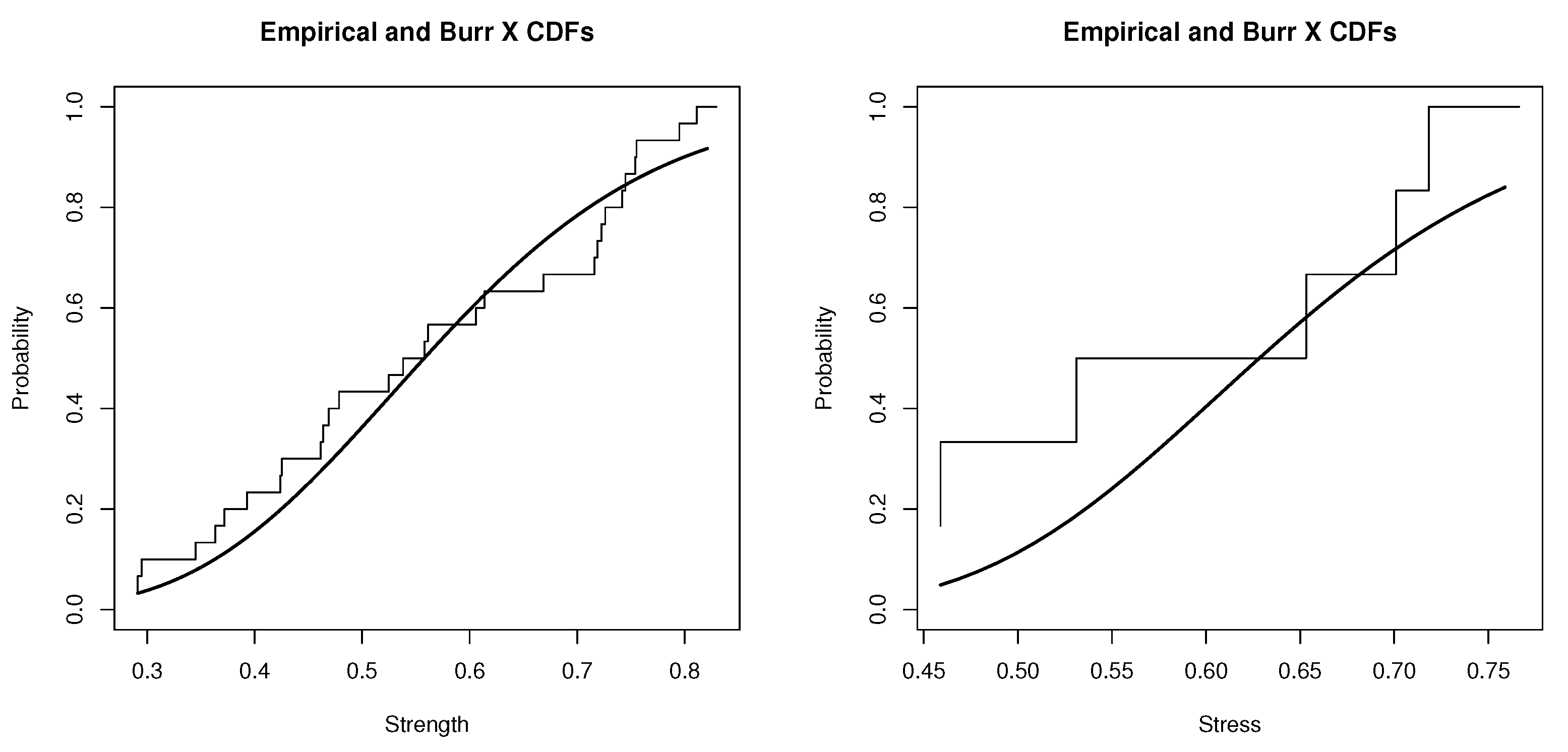
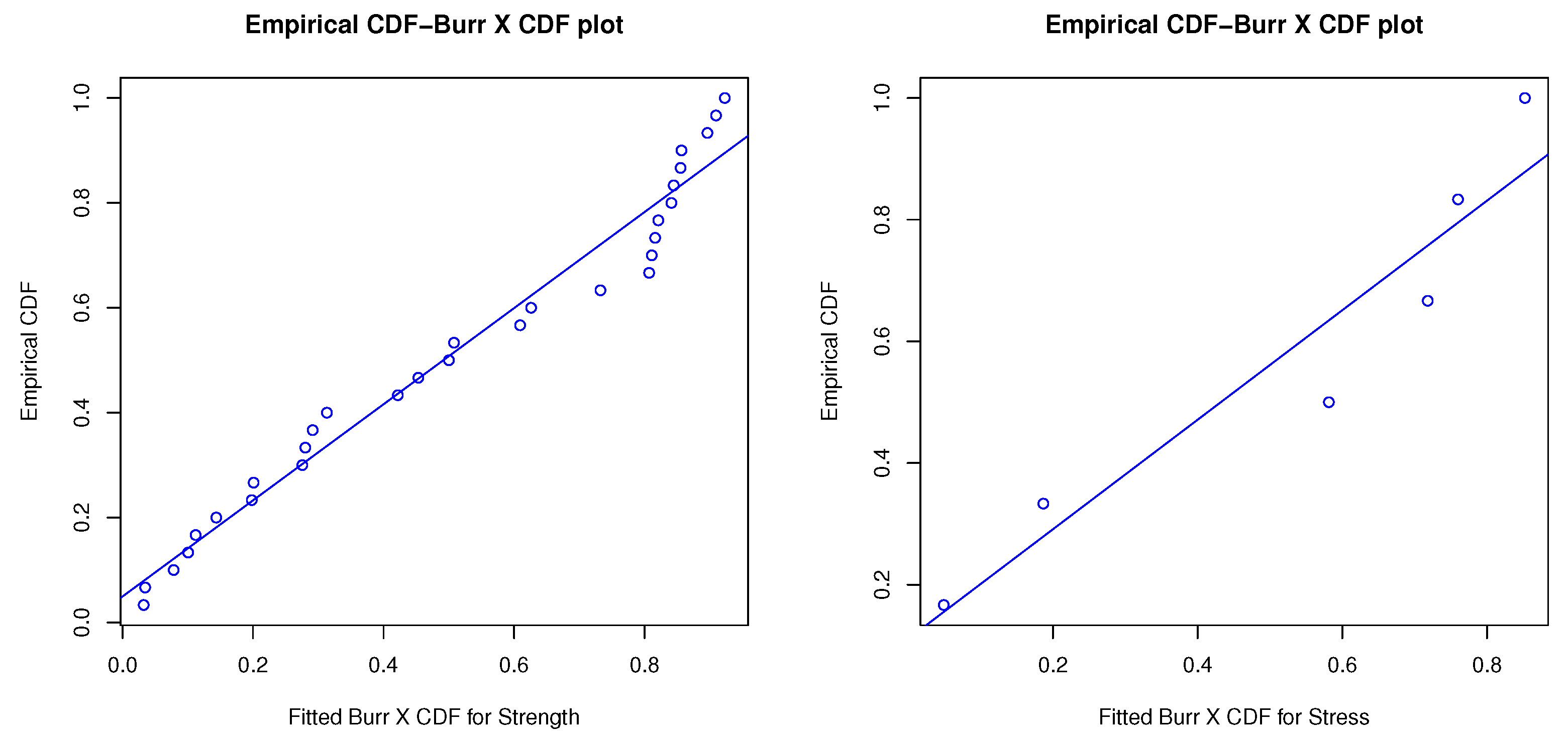
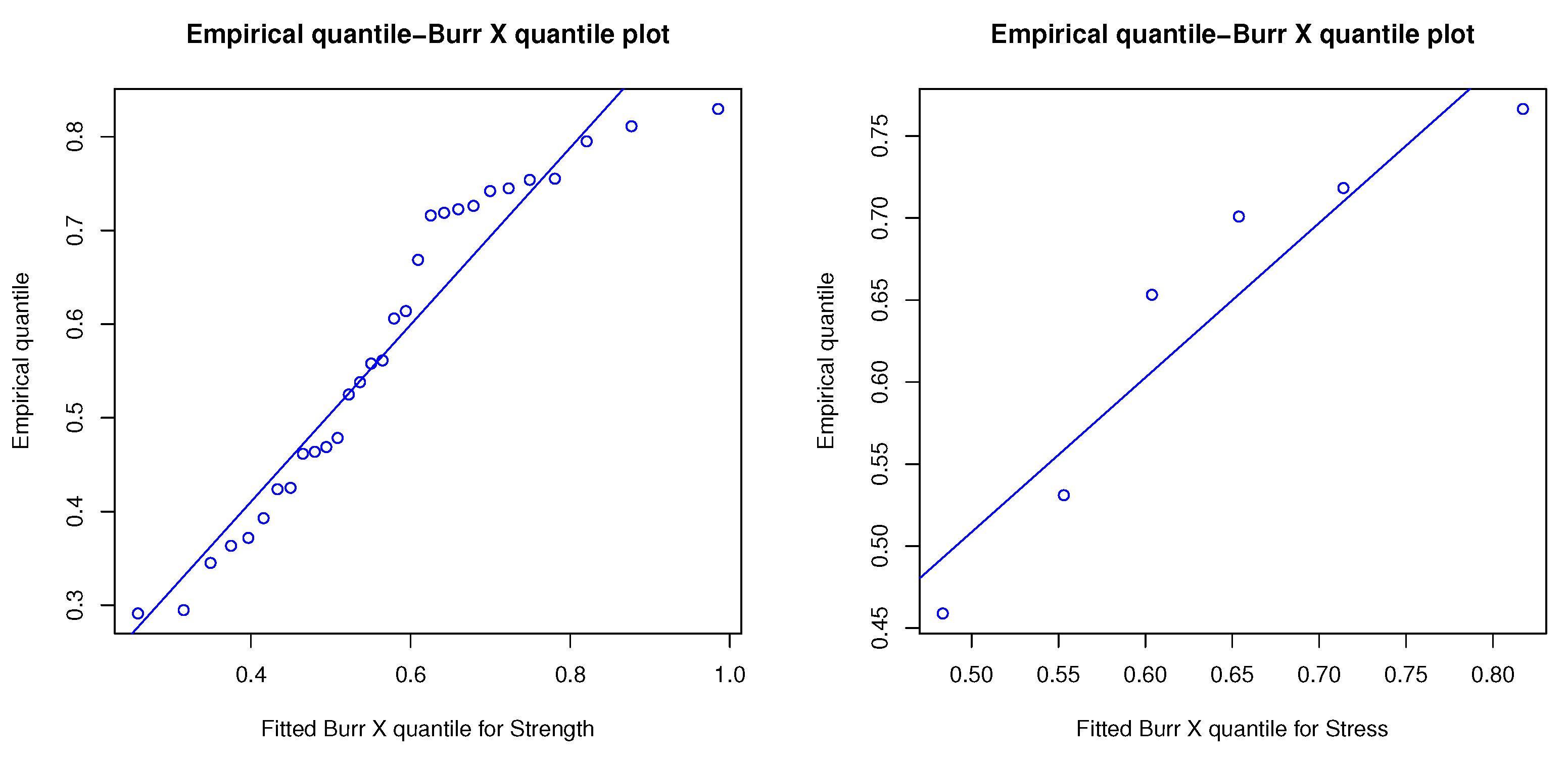
The Kolmogorov–Smirnov (K-S) test of a two-sided rejection region was used to evaluate the Burr X distribution fit of these data sets. The results from the K-S test for the strength and stress data included the following test statistic distances and the corresponding p-values (within brackets): $0.1737\left(0.2907\right)$ and $0.24812\left(0.7771\right)$, respectively. In addition, the overlapped plots of sample empirical cumulative versus Burr X distributions, sample cumulative probability versus Burr X cumulative probability (P-P), and sample quantile versus Burr X quantile (Q-Q) are shown in Figure 1, Figure 2 and Figure 3, respectively. P-P plot is a probability plot for assessing how close a data set fits a specified model or how closely two data sets agree. A Q-Q plot is a graphic method for evaluating whether two data sets come from populations with a common distribution. Figure 2 shows two P-P plots to present the empirical CDFs of the strength sample (left side) and the stress sample (right side) versus the theoretical CDF of Burr X. The imposed linear regressions over P-P plots in Figure 2 were significant, with R-squared values of 0.97 and 0.91 for the complete strength and stress samples, respectively, and the imposed linear regressions over the Q-Q plots in Figure 3 were also significant, with R-squared values of 0.93 and 0.89 for the complete strength and stress samples, respectively. All information reveals that the Burr X distribution was a good fitting probability model for the transformed data sets as well.

Based on the six three-out-of-five G systems provided in this example, the observed data collected from these multicomponent systems are given as follows:

$$\begin{array}{c}\hfill \begin{array}{ccc}\mathrm{Strength}\mathrm{data}\mathrm{of}X& & \mathrm{Stress}\mathrm{data}\mathrm{of}Y\\ \left(\begin{array}{ccc}0.4238& 0.5579& 0.7262\\ 0.2912& 0.3634& 0.3719\\ 0.5381& 0.5612& 0.7226\\ 0.5249& 0.6060& 0.6686\\ 0.3451& 0.4253& 0.4688\\ 0.2948& 0.3929& 0.4616\end{array}\right)& \mathrm{and}& \left(\begin{array}{c}0.7009\\ 0.6532\\ 0.4589\\ 0.7183\\ 0.5310\\ 0.7665\end{array}\right).\end{array}\end{array}$$

The point and interval estimates for the multicomponent system reliability $R_{s,k}$ are shown in

Table 1. The estimation results for $R_{s,k}$ using the collected data from 3-out-of-5 G system.

${\lambda }_1={\lambda }_2$
${\widehat{\mathit{R}}}_{\mathit{s},\mathit{k}}=\mathbf{0.6937}$	${\acute{\mathit{R}}}_{\mathit{s},\mathit{k}}=\mathbf{0.7398}$	${\acute{\mathit{R}}}_{\mathit{s},\mathit{k}}^{\mathit{F}}=\mathbf{0.7836}$
ACI$=(0.4994,0.9635)$	GCI$=(0.4987,0.9506)$	BCI$=(0.4455,0.8923)$
${\lambda }_1\ne {\lambda }_2$
${\check{\mathit{R}}}_{\mathit{s},\mathit{k}}=\mathbf{0.6336}$	${\stackrel{`}{\mathit{R}}}_{\mathit{s},\mathit{k}}=\mathbf{0.4512}$	${\stackrel{`}{\mathit{R}}}_{\mathit{s},\mathit{k}}^{\mathit{F}}=\mathbf{0.4627}$
ACI$=(0.4332,0.9267)$	GCI$=(0.1976,0.7114)$	BCI$=(0.3358,0.8470)$

, where the significance level was set to $0.05$. The estimated interval lengths for ACI, GCI, and BCI were 0.4641, 0.4519, and 0.4468, respectively, when ${\lambda }_1={\lambda }_2$, and 0.4935, 0.5138, and 0.5112, respectively, when ${\lambda }_1\ne {\lambda }_2$. Under ${\lambda }_1={\lambda }_2$, three point estimates were larger than three point estimates under ${\lambda }_1\ne {\lambda }_2$. It was observed that the point estimates were close to each other, except the MLE ${\check{R}}_{s,k}=0.6336$ when ${\lambda }_1\ne {\lambda }_2$. When comparing between all estimated interval lengths, the ACI of $R_{s,k}$ was found to perform equally well in terms of length.

Furthermore, to compare the equivalence between the scale parameters ${\lambda }_1$ and ${\lambda }_2$ from the strength and stress distributions, i.e., null hypothesis $H_0:{\lambda }_1={\lambda }_2$, the likelihood ratio test provided the statistic and p-value of $86.83223$ and $1.18\times {10}^{-20}$, respectively. Hence, the results indicate that under a 0.05 significance level, there is sufficient evidence to reject the null hypothesis. And the strength and stress distributions are suggested to have Burr X distributions with different scale parameters for the current monthly capacity applied. It is worth mentioning that the point estimates of $R_{s,k}$ under different parameters for both Burr X distributions were consistent with the point estimate results of $R_{s,k}$ under the Burr XII distribution modeling studied by Lio et al. [18], where both Burr XII distributions had one common parameter, while the Burr X modeling had different parameters for the same data sets considered.

7. Concluding Remarks

The inference for the multicomponent stress–strength model reliability was investigated using two-parameter Burr X distributions. The maximum likelihood and generalized pivotal quantity based estimators for the model parameters were constructed under equal scale parameters and different scale parameters, respectively. Moreover, confidence intervals were also provided by using the delta method with an asymptotic normal distribution, parametric bootstrap percentile, and generalized pivotal sampling.

Yousof et al. [23] and Jamal and Nasir [24] presented two different Burr X generators based on a one-parameter Burr X distribution. These two types of families have not been applied to estimate the reliability of the multicomponent stress–strength system and can be considered potential future research work. The other possible extension work is to extend the two-parameter Burr X distributions using the same approaches from Yousof et al. [23] and Jamal and Nasir [24]. When the research work is to establish the common goals based on a family of distributions, the model selection based on the Bayesian and likelihood approaches will be reasonably applied and a best model will be used to compare the based model. For more information, readers may also refer to [32,33,34].

Additionally, the present results were established under type II censoring for strength data sets. The approaches could possibly be extended to other censoring; for example, the progressively type-II or progressive first-failure type II censoring scheme with proper modification of pivotal quantities for the related samples. Viveros and Balakrishnan [35] provided more information about progressive censoring schemes. Additionally, the moment and maximum product of spacing estimations are interesting new directions. All of these are potential research opportunities.

References

- Eryilmaz, S. Phase type stress-strength models with reliability applications. Commun. Stat.—Simul. Comput. 2018, 47, 954–963. [Google Scholar] [CrossRef]
- Kundu, D.; Raqad, M.D. Estimation of R = P(Y < X) for three-parameter Weibull distribution. Stat. Probab. Lett. 2009, 79, 1839–1846. [Google Scholar]
- Krishnamoorthy, K.; Lin, Y. Confidence limits for stress-strength reliability involving Weibull models. J. Stat. Plan. Inference 2010, 140, 1754–1764. [Google Scholar] [CrossRef]
- Mokhlis, N.A.; Ibrahim, E.J.; Ibrahim, E.J. Stress-strength reliability with general form distributions. Commun. Stat.—Theory Methods 2017, 46, 1230–1246. [Google Scholar] [CrossRef]
- Surles, J.G.; Padgett, W.J. Inference for P(Y < X) in the Burr Type X Model. J. Appl. Stat. Sci. 1998, 7, 225–238. [Google Scholar]
- Wang, B.; Geng, Y.; Zhou, J. Inference for the generalized exponential stress-strength model. Appl. Math. Model. 2018, 53, 267–275. [Google Scholar] [CrossRef]
- Bhattacharyya, G.K.; Johnson, R.A. Estimation of reliability in multicomponent stress-strength model. Am. Stat. Assoc. 1947, 69, 966–970. [Google Scholar] [CrossRef]
- Dey, S.; Mazucheli, J.; Anis, M.Z. Estimation of reliability of multicomponent stress-strength for a Kumaraswamy distribution. Commun. Stat.—Theory Methods 2017, 46, 1560–1572. [Google Scholar] [CrossRef]
- Kayal, T.; Tripathi, Y.M.; Dey, S.; Wu, S.J. On estimating the reliability in a multicomponent stress-strength model based on Chen distribution. Commun. Stat.—Theory Methods 2020, 49, 2429–2447. [Google Scholar] [CrossRef]
- Kizilaslan, F. Classical and Bayesian estimation of reliability in a multicomponent stress-strength model based on the proportional reversed hazard rate model. Math. Comput. Simul. 2017, 136, 36–62. [Google Scholar] [CrossRef]
- Kizilaslan, F. Classical and Bayesian estimation of reliability in a multicomponent stress-strength model based on a general class of inverse exponentiated distributions. Stat. Pap. 2018, 59, 1161–1192. [Google Scholar] [CrossRef]
- Kizilaslan, F.; Nadar, M. Estimation of reliability in a multicomponent stress-strength model based on a bivariate Kumaraswamy distribution. Stat. Pap. 2018, 59, 307–340. [Google Scholar] [CrossRef]
- Nadar, M.; Kizilaslan, F. Estimation of reliability in a multicomponent stress-strength model based on a Marshall-Olkin bivariate Weibull distribution. IEEE Trans. Reliab. 2016, 65, 370–380. [Google Scholar] [CrossRef]
- Rao, G.S. Estimation of reliability in multicomponent stress-strength model based on Rayleigh distribution. ProbStat Forum 2012, 5, 150–161. [Google Scholar]
- Rao, G.S. Estimation reliability in multicomponent stress-strength based on generalized Rayleigh distribution. J. Mod. Appl. Stat. Methods 2014, 13, 367–379. [Google Scholar] [CrossRef]
- Rao, G.S.; Aslam, M.; Kundu, D. Burr type XII distribution parametric estimation and estimation of reliability of multicomponent stress-strength. Commun. Stat.—Theory Methods 2015, 44, 4953–4961. [Google Scholar] [CrossRef]
- Shawky, A.I.; Khan, K. Reliability estimation in multicomponent stress-strength based on inverse Weibull distribution. Processes 2022, 10, 226. [Google Scholar] [CrossRef]
- Lio, Y.L.; Tsai, T.-R.; Wand, L.; Cecilio Tejada, I.P. Inferences of the Multicomponent Stress-Strength Reliability for Burr XII Distributions. Mathematics 2022, 10, 2478. [Google Scholar] [CrossRef]
- Sauer, L.; Lio, Y.; Tsai, T.-R. Reliability inference for the multicomponent system based on progressively type II censoring samples from generalized Pareto distributions. Mathematics 2020, 8, 1176. [Google Scholar] [CrossRef]
- Wang, L.; Lin, H.; Ahmadi, K.; Lio, Y. Estimation of stress-strength reliability for multicomponent system with Rayleigh data. Energies 2021, 14, 7917. [Google Scholar] [CrossRef]
- Burr, I.W. Cumulative frequency functions. Ann. Math. Stat. 1942, 13, 215–232. [Google Scholar] [CrossRef]
- Belili, M.C.; Alshangiti, A.M.; Gemeay, A.M.; Zeghdoudi, H.; Karakaya, K.; Bakr, M.E.; Balogun, O.S.; Atchade, M.N.; Hussam, E. Two-paramter family of distributions: Properties, estimation, and applications. AIP Adv. 2023, 13, 105008. [Google Scholar] [CrossRef]
- Yousof, H.M.; Afify, A.Z.; Hamedani, G.G.; Aryal, G. The Burr X generator of distributions for lifetime data. J. Stat. Theory Appl. 2017, 16, 288–305. [Google Scholar] [CrossRef]
- Jamal, F.; Nasir, M.A. Generalized Burr X family of distributions. Int. J. Math. Stat. 2018, 19, 55–73. [Google Scholar]
- Jaheen, Z.F. Empirical Bayes estimation of the reliability and failure rate functions of the Burr type X failure model. J. Appl. Stat. Sci. 1996, 3, 281–288. [Google Scholar]
- Ahmad, K.E.; Fakhry, M.E.; Jaheen, Z.F. Empirical Bayes estimation of P(Y < X) and characterization of Burr-type X model. J. Stat. Plan. Inference 1997, 64, 297–308. [Google Scholar]
- Akgul, F.G.; Senoglu, B. Inferences for stress-strength reliability of Burr type X distributions based on ranked set sampling. Commun. Stat.—Simul. Comput. 2022, 51, 3324–3340. [Google Scholar] [CrossRef]
- Efron, B. Jackknife, Bootstrap, Other Resampling Plans. In CBMS-NSF Regional Conference Series in Applied Mathematics; SIAM: Philadelphia, PA, USA, 1982; Volume 38. [Google Scholar]
- Hall, P. Theoretical comparison of bootstrap confidence intervals. Annu. Stat. 1988, 16, 927–953. [Google Scholar] [CrossRef]
- Xu, J.; Long, J.S. Using the Delta Method Tonconstruct Confidence Intervals for Predicted Probabilities, Rates, and Discrete Changes; Lecture Notes; Indiana University: Bloomington, IN, USA, 2005. [Google Scholar]
- Weerahandi, S. Generalized Inference in Repeated Measures: Exact Methods in MANOVA and Mixed Models; Wiley: New York, NY, USA, 2004. [Google Scholar]
- Cherstvy, A.G.; Thapa, S.; Wagner, C.E.; Metzler, R. Non-Gaussian, non-ergodic, and non-Fickian diffusion of tracers in mucin hydrogels. Soft Matter 2019, 15, 2526–2551. [Google Scholar] [CrossRef]
- Thapa, S.; Park, S.; Kim, Y.; Jeon, J.-H.; Metzler, R.; Lomholt, M.A. Bayesian inference of scaled versus fractional Brownian motion. J. Phys. A Math. Theor. 2022, 55, 194003. [Google Scholar] [CrossRef]
- Krog, J.; Lomholt, M.A. Bayesian inference with information content model check for Langevin equations. Phys. Rev. E 2017, 96, 062106. [Google Scholar] [CrossRef] [PubMed]
- Viveros, R.; Balakrishnan, N. Interval estimation of parameters of life from progressively censored data. Technometrics 1994, 36, 84–91. [Google Scholar] [CrossRef]
- Lawless, J.F. Statistical Models and Methods for Lifetime Data, 2nd ed.; Wiley: New York, NY, USA, 2003. [Google Scholar]
- Stephens, M.A. Tests for the exponential distribution. In Goodness-of-Fit Techniques; D’Agostino, R.B., Stephens, M.A., Eds.; Marcel Dekker: New York, NY, USA, 1986; pp. 421–459. [Google Scholar]
Figure 1.
Step figure is the sample empirical distribution and curve is the fitted Burr X distribution. Left side is for strength data modeling with BurrX. Right side is for stress data modeling with BurrX.
Figure 2.
Sample cumulative probability vs. Burr X cumulative probability plot overlapped with the regression line. Left side is for strength data modeling with BurrX and fitting regression line with R2 = 0.97. Right side is for stress data modeling with BurrX and fitting regression line with R2 = 0.91.
Figure 3.
Sample quantile vs. Burr X quantile plot overlapped with the regression line. Left side is for strength data modeling with BurrX and fitting regression line with R2 = 0.93. Right side is for stress data modeling with BurrX and fitting regression line with R2 = 0.89.