On the Modeling of Ship Stiffened Panels Subjected to Uniform Pressure Loads


Shipbuilding Technology Laboratory, School of Naval Architecture and Marine Engineering, National Technical University of Athens, 9 Heroon Polytechniou Av., Zografos, 15780 Athens, Greece
*
Author to whom correspondence should be addressed.
Appl. Mech. 2022, 3(1), 125-143; https://0-doi-org.brum.beds.ac.uk/10.3390/applmech3010010
Submission received: 7 January 2022
/
Revised: 27 January 2022
/
Accepted: 28 January 2022
/
Published: 1 February 2022
(This article belongs to the Special Issue Mechanics and Control using Fractional Calculus)
Abstract
:Stiffened panels constitute structural assemblies of the entire ship hull, i.e., double bottom, side shell, deck areas, etc. Prescriptive dimensioning of the stiffeners (web thickness and height and flange thickness and breadth) is solely based on the application of beam bending theories. This work is divided into two parts. The first part involves the assessment of the structural response of one-way (single-bay) stiffened panels under uniform pressure. The objective is to evaluate the effectiveness of alternative approaches in obtaining accurate secondary stress fields. Both state-of-the-art analytical solutions (Paik, Schade, CSR, Miller) and numerical calculation tools (finite element analysis (FEA)) are employed and compared for this purpose. When it comes to cross-stiffened panels, numerical methods are usually used within the design process which is time demanding. The second part of this work focuses on the development of a fast, yet effective, prescriptive approach. This approach will allow the dimensioning of the longitudinal stiffeners by considering the secondary stress field. Combining finite element analysis and the Euler–Bernoulli bending theory, the effect of the transverse stiffeners to the longitudinal stiffeners is examined in order to estimate the type of support on the boundaries of the transverse stiffeners. Determining the type of support, will make it possible to apply the classical formula of bending stress instead of using finite element analysis, thus limiting the computational cost. Preliminary calculations show that most of the examined cases may be treated as fully clamped beams subjected to uniform pressure.
1. Introduction
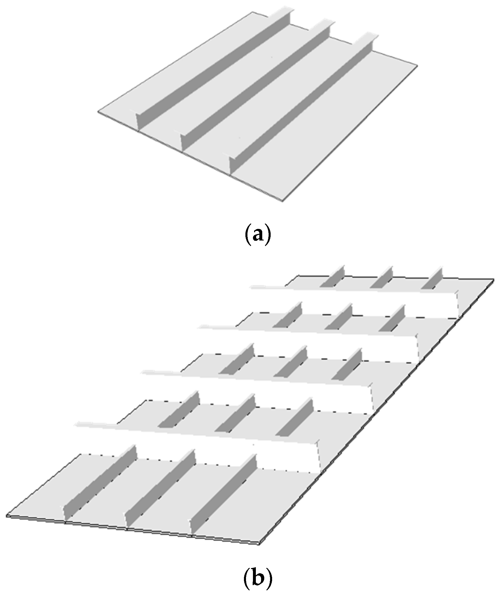
Stiffness and strength resistance of marine constructions is assessed through the application of strategies and theories for thin-walled slender structures, since they are built by open or closed cell arrangements of welded plates. Relatively stiff composite beam profiles are welded on platings to counteract the low inherent slenderness of the platings. Local dimensioning of ship hull structures (thicknesses, spacings, profiles, etc.) is based upon a design process of elementary sections that form a structural unit denoted as a stiffened panel. It is typical to find unstiffened panels (stiffeners are placed only along one main dimension) in almost all areas of bulkers, tankers and containerships, as shown in Figure 1a. Car carriers and passenger ships have several twin decks which are mostly cross-stiffened, i.e., groups of stiffeners of different rigidity are placed in both main directions of the stiffening area (see Figure 1b). The level of stiffening and selected scantlings results from specifications and constraints posed in the design, erection, operation and maintenance phases. In ship hull structures, dimensioning of stiffened panels with respect to elastic analysis seems to result at higher scantling requirements compared to dimensioning against structural instability (buckling), [1]. Therefore, by employing elastic design followed by buckling assessment, design iterations that require important modifications in structural arrangement and geometry are eliminated.
For elastic design, local loads (e.g., hydrostatic and hydrodynamic pressure) combined with global loads (hull girder load effects) are taken into consideration [2]. Hull girder bending and torsion stress effects, known as principal stresses, σ1, are usually thought to have a certain linear distribution along the ship’s depth (distance z) in the beginning of the design. This may be calculated by assuming that the neutral axis (NA) of the ship’s transverse section is typically located somewhere between 30–40% of the ship’s molded depth, measured from the bottom-line and taking into consideration an optimal design where the deck is fully utilized. Principal normal stresses are described by Navier’s bending formula as:
where Mhg and Ihg correspond to the hull-girder bending moment and hull-girder moment of inertia at a given longitudinal station, respectively.
From the local perspective, bending stresses produced by pressure loads are engineering wise split into the generation of secondary (σ2) and tertiary stresses (σ3). The latter are generated due to the double curvature of the unstiffened (unsupported) plate area, and plate bending theories (Love, Mindlin, etc.) may well be applied. Secondary stresses develop because of the bending curvature of the stiffener with its attached plating, and beam theories apply accordingly, i.e., Euler, Navier, Timoshenko, etc. In general, one cannot expect that the actual stress state is equal to σ1 + σ2 + σ3, and for this purpose the notion of such stress decomposition is used in dimensioning of stiffened panels in an uncoupled fashion, [3]. Once stiffener spacing is predefined, plate bending theory (or sometimes elastoplastic beam bending of a strip of the plate taken from the short dimension of the plate) is used for calculating the minimum required thickness of a certain plate, tp, as per CSR, which corresponds at the tertiary stress analysis:
where αp is a correction factor, s is the stiffener spacing, P is the applied pressure, χ and Ca are coefficients and REh is the permissible material resistance. In ship structural design, as dictated by the rules and common industrial practice, dynamic loads arising from, e.g., waves are treated as static loads with the use of partial safety factors. This strategy is considered herein as well.
The periodicity (symmetry) in the stiffened panel geometry of Figure 1 is accompanied by periodicity in the stress field of the stiffened panel which in turn allows for solving the problem in one dimension, i.e., by considering a beam with an effective and representative cross-section and applying the bending theory. The elastic resistance of a given stiffener (profile and scantlings) is assessed through the application of secondary stresses, by defining a minimum section modulus requirement, Zmin:
where lbdg is the effective beam span, and fbdg and Cs are coefficients.
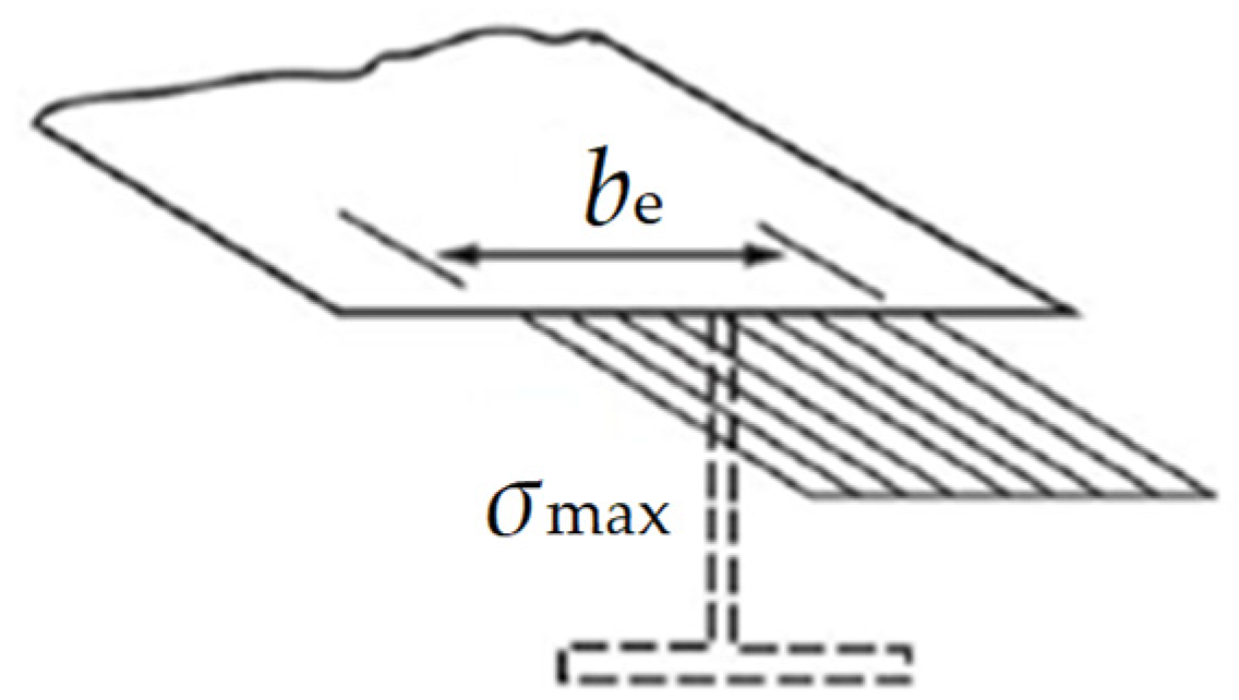
The corresponding cross-section used in the beam analysis for comparing against Equation (3) needs to be defined. Periodicity implies that the attached plating with width equal to the stiffener spacing, s, is a geometric calculation that may overestimate the panel’s strength. The reason for the overestimation is associated with the phenomenon of shear lag which pollutes the uniformly distributed normal stress field assumed by classical bending theory, Timoshenko and Goodier (1951). This is because the Euler–Bernoulli bending theory of beams ignores the warping of the elements of the cross-section due to the shear stresses, which give rise to an axial warping stress field. The reason is that uniform pressure loads lead to the creation of both axial bending stresses and shear stresses that distort the cross-section. As a result, the real distribution along the section’s width is nonuniform. This phenomenon is referred to as shear lag, and it is dominant in thin-walled sections with elements having at an angle between them. Hence, a correction that takes into account the shear lag effect at reduced effective widths is introduced. The notion of the effective width is introduced, denoted as be, where only part of the stiffener spacing (be < s) carries the otherwise nonuniform secondary bending stresses, in a uniform manner as illustratively shown in Figure 2.
Once the real nonuniform bending stressdistribution, σx, is derived by modeling the shear lag effect, employment of static equilibrium over the attached plating results inthe following formula, [4]:
where σmax is the maximum stress found within the integral bounds and is applied at the effective width of the stiffened plate (reduced spacing). With be known, the actual section modulus of the stiffener with the effective attached plating may be easily calculated.
It is evident that knowledge of the plate’s effective width allows for the application of the classical bending theory. In practical design there is no need to find the real stress distribution to apply Equation (4) but be is given with respect to other stiffener dimensions. However, different approaches for assessing the shear lag problem and hence arriving at different effective width values do exist in the literature. Traditional works date back to the 1950s with the pioneering efforts of [5] in general mechanics and by Schade [6] in naval architecture. Though shear lag is an old problem, there is still ongoing research in the field that has applications in civil infrastructure apart from naval architecture. Some indicative works published within the past 20 years are presented in [7,8,9,10,11,12,13,14] and Miller (1976) (The formulation and analysis in Miller (1976) is provided in detail and referenced accordingly to Miller’s solution in the book of P. Caridis, Strength Analysis of Ship Structures, 2017, Caridis publishing.). Some recent works are presented in [15,16,17].
The current work has a twofold objective with special focus on the elastic strength analysis of one-way (single-bay) and cross-stiffened panels. The first objective is associated with the assessment of four approaches (two analytical, one semiempirical and one rule-based) that tackle the shear lag problem and allow for the application of Equation (4), hence resulting in four alternative effective width relations. Finite element simulations were performed in order to consider reference results for comparison purposes. An additional semianalytical calculation model for the effective width was produced based on fitting polynomials on complex closed-form solutions. The second objective is to simplify the strength analysis of cross-stiffened panels by considering a reduced one-dimensional problem, where the rotational stiffness posed by the transverse stiffeners is mathematically modeled. The question that is to be answered is the identification of the relation between the stiffener’s rigidity which will be imposed as boundary restraints to the beam ends under analysis. This problem is tackled through FEA and metamodeling.
2. One-Way (Single-Bay) Stiffened Panel
Based on one-way (single-bay) stiffened panels, this section deals with the assessment of four approaches used in the analysis of the shear lag problem and consequently arrives at descriptions of the calculation of the effective width used in stiffened panels. Corresponding formulas found in [2,3,4] are selected for comparison purposes. These specific works are chosen as the most popular ones cited in textbooks and class rules.
2.1. Analytical Solution of Miller
The following approach that was initially proposed by Miller (1976) [4], is to the authors’ best knowledge the most intuitive one with respect to the employed rules of mechanics that describe the involved physical mechanisms well. The normal stress field corrected for shear distortions (shear lag effect) is given by the linear superposition of the following magnitudes.
Magnitude σb(z) denotes the bending axial stresses (σb = Μz/Ι). Detailed derivation of σshearlag(x,s) is provided in Appendix A. Superposition of the preceding magnitudes does not guarantee equilibrium of forces and moments. For this reason, the out of balance equivalent force and moment counterparts may be calculated as:
2.2. Alternative Analytical Solutions
The most common analytical solutions used within the analysis and design of stiffened panels are from [3]. The classical theory of elasticity is applied as per Timoshenko and Goodier (1951) in [5]. A 2D stress state has been considered within the section’s elements. The compatibility equation has been solved for the Airy’s stress function. Stiff transverse frames have been considered, and harmonic solutions to the displacement field have been undertaken. A uniform pressure has been considered as well. Eventually the obtained stress field maximum value and distribution have been used within Equation (4) to generate an expression for the notion of the effective breadth of the attached plating as given below:
The rule-based design as per Common Structural Rules (CSR 2021) provides the following expression for the effective width to be considered in the analysis:
As per the technical background of the CSR, the preceding equation is obtained based on the theoretical work performed in [6,18]. It is stated that FE simulations have been used to verify the equations.
Schade’s expression is provided in a curve form [1] where an analytical solution based on the theory of elasticity is applied again by considering a 2D stress field.
2.3. Assessment of Analytical Solutions
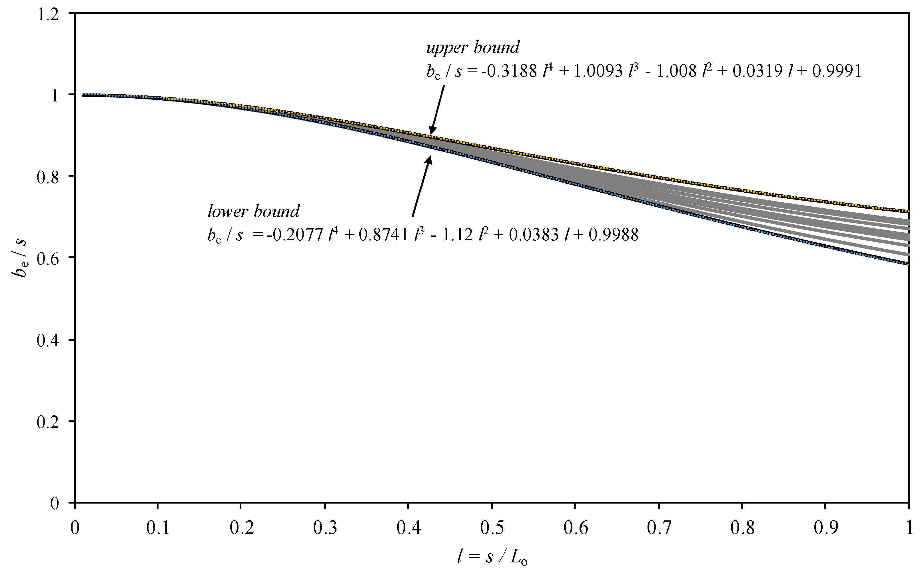
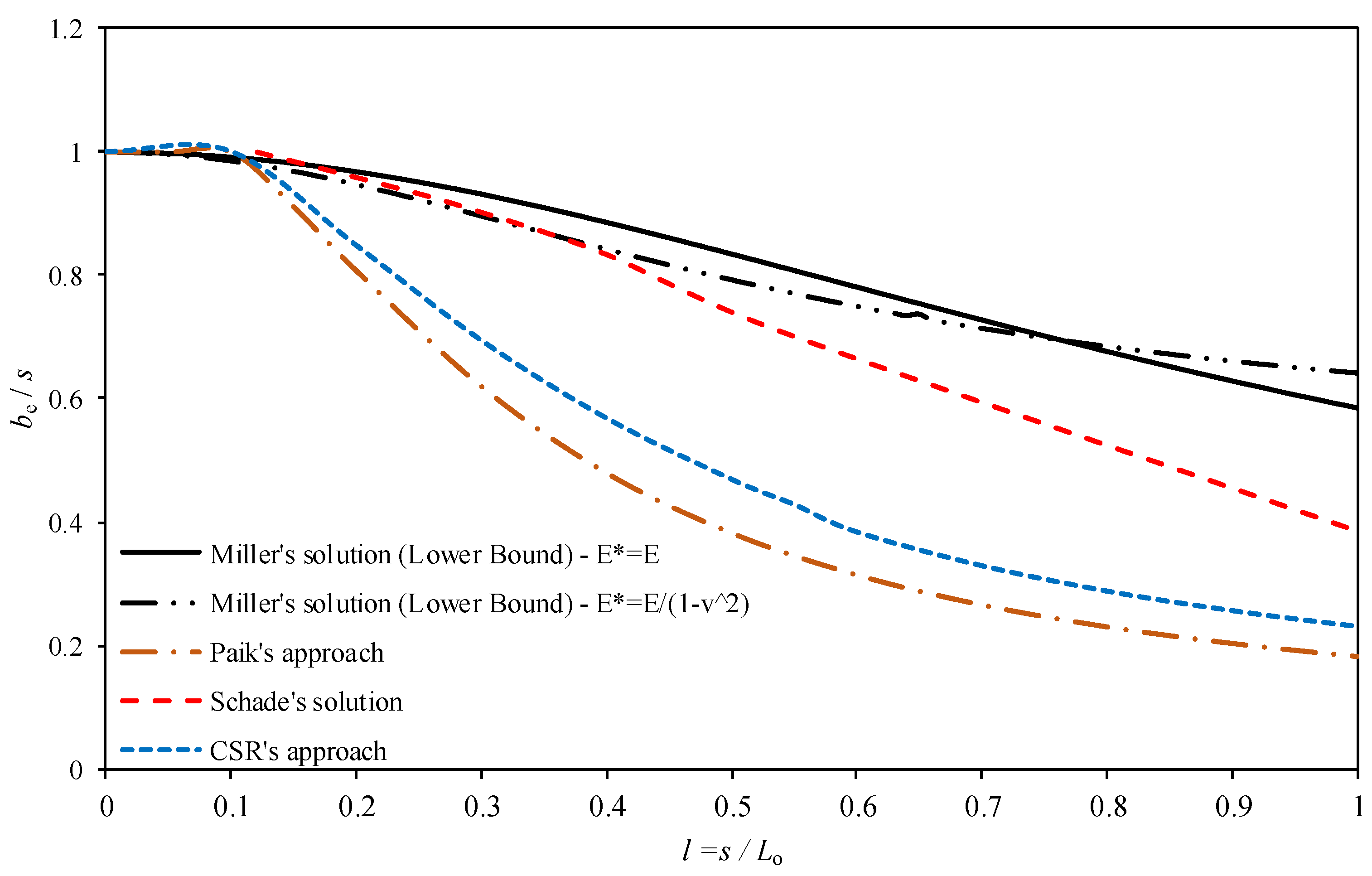
Miller’s solution is not directly generalized to provide relations in the form be/s = f(s/L). In this respect, a representative sample of 10 realistic scantlings was taken from bulk carriers and tankers. Table 1 lists corresponding dimensions for T shape profiles and corresponding spacing and plate thickness. For each single case, the formulation provided in Section 2.1 was applied and the corresponding real stress field was evaluated through Equation (6). The maximum stress σmax was identified and consequently Equation (4) was applied to derive the effective width per case. The corresponding results are plotted in Figure 3 for all 10 cases. For practical purposes the lower and upper bound solutions (envelope) have been fitted with quartic polynomials that yield an R-squared statistic almost equal to unity through the method of least squares. Each curve corresponds to specified scantlings as given in Table 1 and is numerically generated, i.e., a closed-form solution of the be/s = f(s/Lo) is not provided. However, to produce an analytical formula for each case, a polynomial was used. The lower bound corresponds to the case that has yielded the lowest effective width. This has been done in an effort to generalize over the population from the sample of the 10selected cases. The lower bound could be potentially used for design purposes. Figure 4 compares Miller’s solution with the corresponding ones obtained by Paik (Equation (9)), CSR (Equation (10)) and Schade’s solution digitized from [1]. It is evident that there are significant differences between each case, showing the ambiguity of precisely defining the effective width for describing the secondary normal bending stresses.
The following section is dedicated to providing a comparative assessment of the effectiveness of each employed method for obtaining the effective width of a stiffened panel with a special focus on stiffened panels with T profile sections.
2.4. Assessment of the Analytical Solutions
As already mentioned, the notion of secondary stresses is an engineering approach used in the dimensioning process of stiffened panels. Therefore, identifying the correct effective width magnitude is not always a straightforward procedure, since tertiary and secondary stresses develop simultaneously.
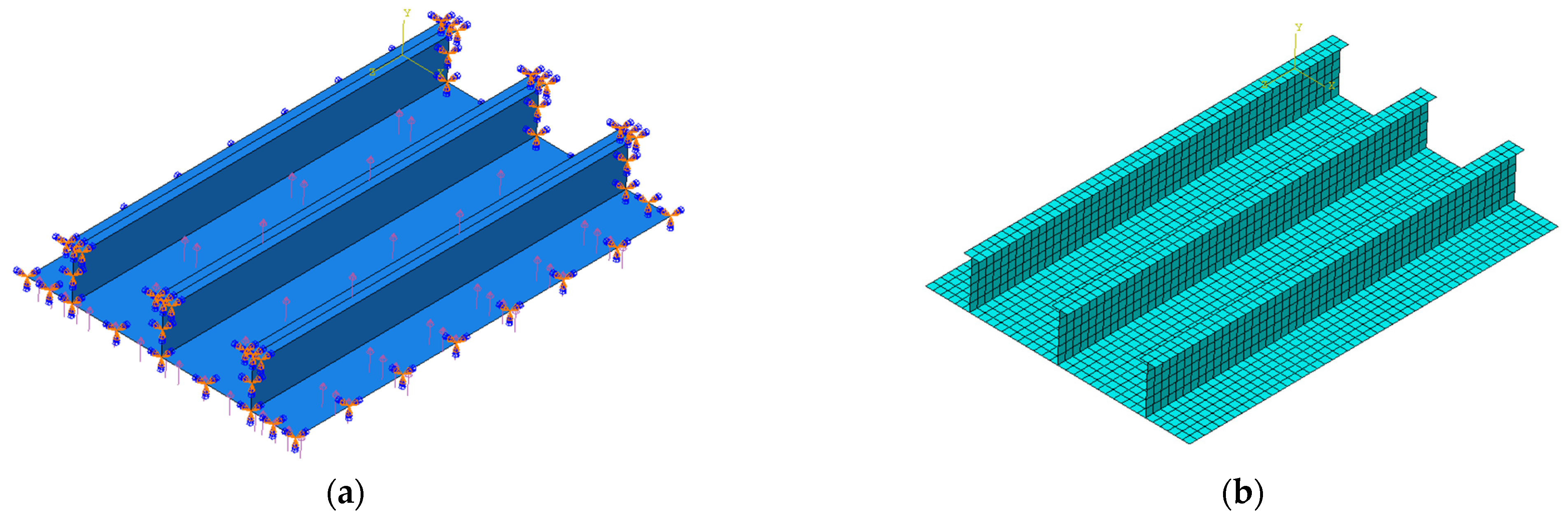
To provide a quantitative comparison among the four considered approaches in this work, corresponding results from a finite element (FE) analysis have been considered to act as a reference case. Two stiffened-panel geometries taken from an actual bulk carrier with 180,000 TDW (292 m overall length), were modeled to serve this purpose. Both panels are stiffened with “Tee” profile stiffeners. Three longitudinal stiffeners exist between the girders of the double bottom. One panel comes from the bottom plating of the vessel (475 × 9 + 150 × 15, plate thickness = 19.5 mm, stiffener spacing = 850 mm and floor spacing = 3700 mm), and one comes from the topside wing tank (450 × 9 + 150 ×18, plate thickness = 26 mm, stiffener spacing = 905 mm and floor spacing = 5550 mm). The FE model was constructed in Abaqus implicit. Quadratic 8-node shell elements with quadrilateral shape were used for the plating and stiffeners with linear elastic material behavior (E = 207 GPa, v = 0.3).Following a convergence study, the selected finite element dimensions were taken equal to (75 × 75) mm2, that is, half the flange breadth. The midsurface of the panel was modeled. All nodes of all degrees of freedom lying at the boundary of the modeled geometry were set to zero, corresponding to a fully clamped support condition. A uniformly distributed static pressure of magnitude 0.1 MPa was applied over the plate (hydrostatic pressure). The loads, BCs and mesh of the bottom stiffened panel are shown in Figure 5.
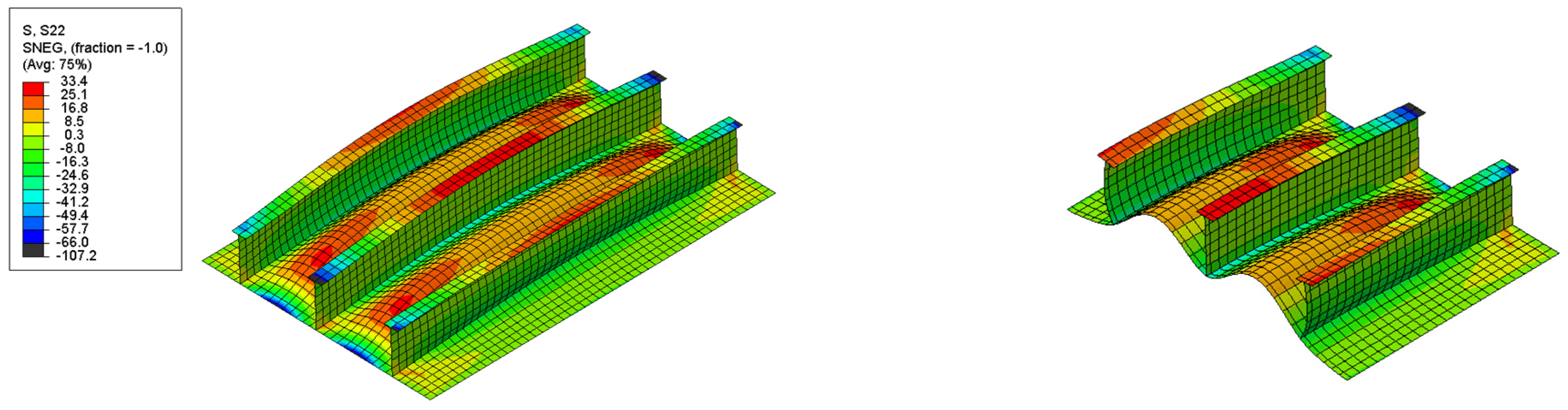
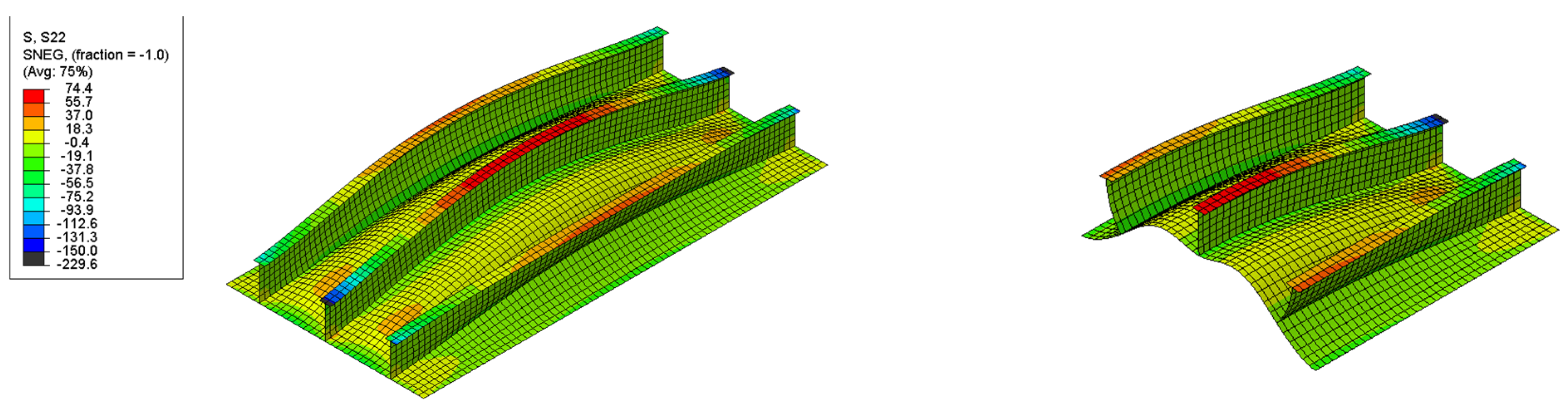
Figure 6 and Figure 7 present the distribution of the normal bending stress along the stiffeners’ direction that is produced as a consequence of the pressure load. It is evident that the stress field is almost periodic for the three stiffeners. The middle stiffener is considered the representative one, because it is not that affected by the imposed boundary conditions applied at the edges. Within the unsupported region between the stiffeners, tertiary (plate bending stress field) and secondary stresses are superimposed. Hence it is difficult to separate them. However, it is assumed that the axial bending stress developed at the flange is purely associated with the secondary stress field and unaffected by the tertiary stresses. According to statics, the bending moment developed at a fixed-fixed beam subjected to uniform line load is maximum at the supports (magnitude equal to qL2/12, where q stands for the line load and L stands for the beams span) and half of that moment is developed at the midspan (magnitude equal to qL2/24) but with opposite curvature (i.e., sign). This qualitative appreciation compares well with the corresponding FEA results as the normal stress at the midspan at the flange is approximately half that obtained in the vicinity of the supports. However, there does exist a stress concentration exactly at the supports that is attributed to the constraint itself, which pollutes the theoretical notion of the secondary stresses. To remove this boundary effect, the normal stress calculated at midspan, i.e., 33.4 MPa for the bottom panel (see Figure 6) and 74.4 MPa for the topside wing tank panel (see Figure 7), were considered as the most accurate representations of the secondary stress calculated through FEA. Therefore, the maximum secondary stress was taken as double the aforementioned values, that is 66.8 MPa and 148.8 MPa for the bottom and top panel, respectively. These levels were then compared with the corresponding results obtained by employing Equation (5) for each alternative effective width (Paik, CSR, Schade and Miller lower bound) and then employing Equation (1) to derive an analytical value.
Table 2 and Table 3 list the percentage difference between the maximum secondary stress from FEA and the respective analytical stress value. It is evident that the difference varies within the range 6–13%, and consequently, one could say that this range is not statistically significant. It is surprising that although there is quite a difference in the calculated effective widths per employed method, this difference does not propagate to the maximum normal stress. The magnitude that controls the stress is the section modulus (Equation (5)) where be has an important role. However, as the effective width decreases, the neutral axis (NA) moves further away from the attached plating, and there is an interplay between the moment of inertia and the NA location. Eventually, the effective cross-section does not significantly vary with the alternative effective width magnitudes. For instance, for the bottom panel by assuming that the effective width is 35% of the spacing, the resulting stress differs by 6% based on the FEA result. If we consider that the effective width is 81% of the spacing, then the difference is ~12%, still not that significant. Though more cases (extensive parametric studies) should be examined to draw a concrete conclusion, it is evident that in practical design, all four approaches might effectively be used along with a calibrated factor of safety against computational uncertainties.
3. Simplifying the Analysis of Cross-Stiffened Panels
This section has a special focus on the dimensioning process of cross-stiffened panels, i.e., stiffening at both in-plane directions. In the shipbuilding industry, cross-stiffened panels are found mainly in passenger and RORO vessels, among other class types. For dimensioning purposes of the stiffeners and the plate, usual engineering practice involves the application of numerical methods, which is time demanding. Our aim is to simplify the geometry in order to successfully dimension the longitudinal stiffeners by solely considering the secondary stress field. Namely, the scope is to reduce the model’s geometry to a one-dimensional problem, which will allow for the application of the classical beam bending theory. However, the presented simplification approach only applies to cases where the transverse stiffening is strong (e.g., deck in bulkers/tankers) related to the longitudinal stiffening.
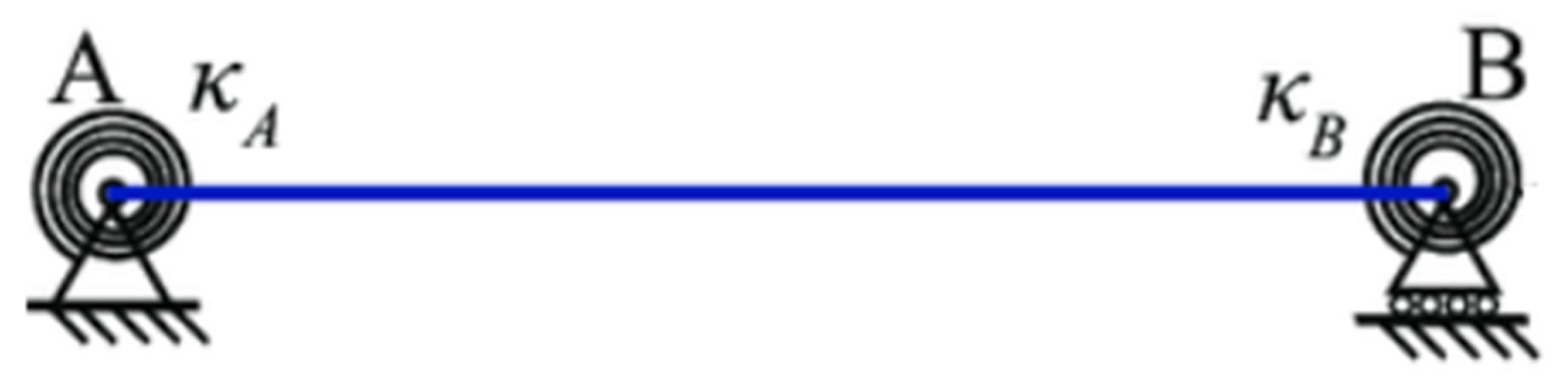
To calculate the stress field for a longitudinal stiffener based on a one-dimensional analysis, we need to estimate the type of support that is imposed at the stiffener connections due to the existence and cooperation of/with the transverse stiffening system. The proposed concept involves determining the secondary normal bending stresses by introducing a phenomenological stiffness coefficient, namely k, which implicitly models the rotational rigidity of the transverse stiffeners. Figure 8 illustrates the concept. It must be clarified that the stiffness coefficient k is not equivalent to the spring torsional constants (κ1, κ2) but is associated with the produced load effect. A transverse stiffener of high rigidity produces higher reactive moment when a relative rotation is exerted. The extreme case is when rotational stiffness is at high levels and therefore rotation is not allowed at all. This case leads at a fully clamped beam case subjected to a uniform line load, that produces the bending effect M given by the following equation:
where k takes the value of 12 at the ends, as already mentioned. On the other hand, if the transverse stiffener has a quite weak torsional rigidity, then the ends of the one-dimensional longitudinal stiffener model are free to rotate without any constraint. In this particular case, the maximum bending moment develops at the midspan, and k takes the value of 8. The bending stress formula is then given as:
where I is the moment of inertia and Z is the section modulus of the effective cross-section (with the attached plating) of the longitudinal stiffeners and zmax is the distance of the most remote material fiber (flange). This study works on deriving a correlation between the sectional property of the transverse stiffener and parameter k.
3.1. Design of Experiment and Test Matrix
To achieve reliable results, we needed to run the model for a range of parameters. The choice of the values of the parameters, were determined from the Central Composite Design (CCD), that is a design space exploration technique that sources from Design of Experiments (DoE).
Central composite design was appropriate for calibrating full quadratic models. It consisted of a full factorial design with a central point and additional axial points at a specific distance from its center. For our model, the faced design was used. The range of the values of the variables were determined from the range of the values that were used in actual ship scantlings. The variables of the model were the transverse stiffener spacing, st, the longitudinal stiffener spacing, s, the plate thickness, tp, and the second moment of inertia of the longitudinal profile, Is.
Considering that n represents the number of variables, the total number of design points was equal to 2n + 2n + 1 which was equal to 25 for n = 4. The range of the values for the variable st was selected from 1800 to 5400 mm, for the variable s from 600 to 900 mm and for the variable tp from 12 to 28 mm. For the variable Is the “Tee” profiles were the following: (200 × 10 + 50 × 10), (280 × 14 + 90 × 14) and (340 × 15 + 110 × 15). Consequently, the test matrix of these four variables is listed in Table 4.
In order to examine the effect of the transverse stiffeners on the secondary stress field, for each of the above 25 cases, the coefficient k was calculated for five different cross-sections of transverse stiffeners. Table 5 presents the selected stiffener combinations used in setting up the numerical experimentalprogram.
The dimensions of the transverse stiffeners were chosen considering that the second moment of inertia of longitudinal stiffeners is smaller than the second moment of inertia of transverse stiffeners, as usually found in ships. Moreover, for each case, all structural elements comply with the rule-based slenderness and proportion requirements.
3.2. Finite Element Modeling
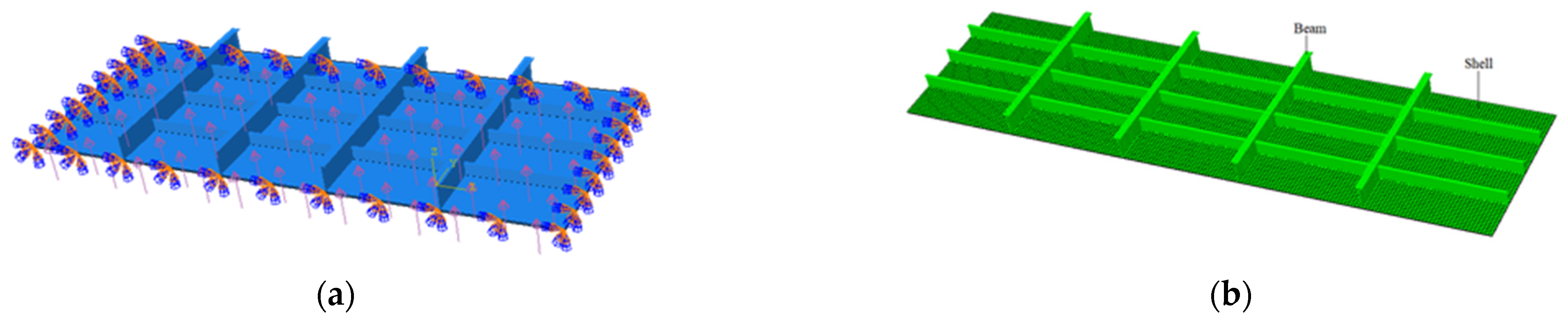
For each discrete case, a corresponding FE model was developed with a given geometry extent. To avoid any model and constraint-based numerical errors, a cross-stiffened panel consisting of four transverse stiffeners with spacing equal to st and three longitudinal stiffeners with spacing equal to s was used. We were interested in the middle longitudinal stiffener located between the two central transverse stiffeners. Typically, girders and floors are found on the boundaries of cross-stiffened panels. As such, the boundary of the modeled geometry was considered as fully clamped, i.e., all DoFs of all boundary nodes was constrained. A uniform pressure with magnitude equal to 0.1 MPa was applied. Figure 9a shows the geometry and applied loads and BCs. A steel material with linear elastic behavior (E = 207 GPa and v = 0.3) was considered. The plate was modeled with linear 4-node shell elements and the stiffeners with 2-node beam elements. A structured mesh consisting of (50 × 50) mm2 quadrilaterals and line elements was eventually constructed per case, as indicatively shown in Figure 9b.
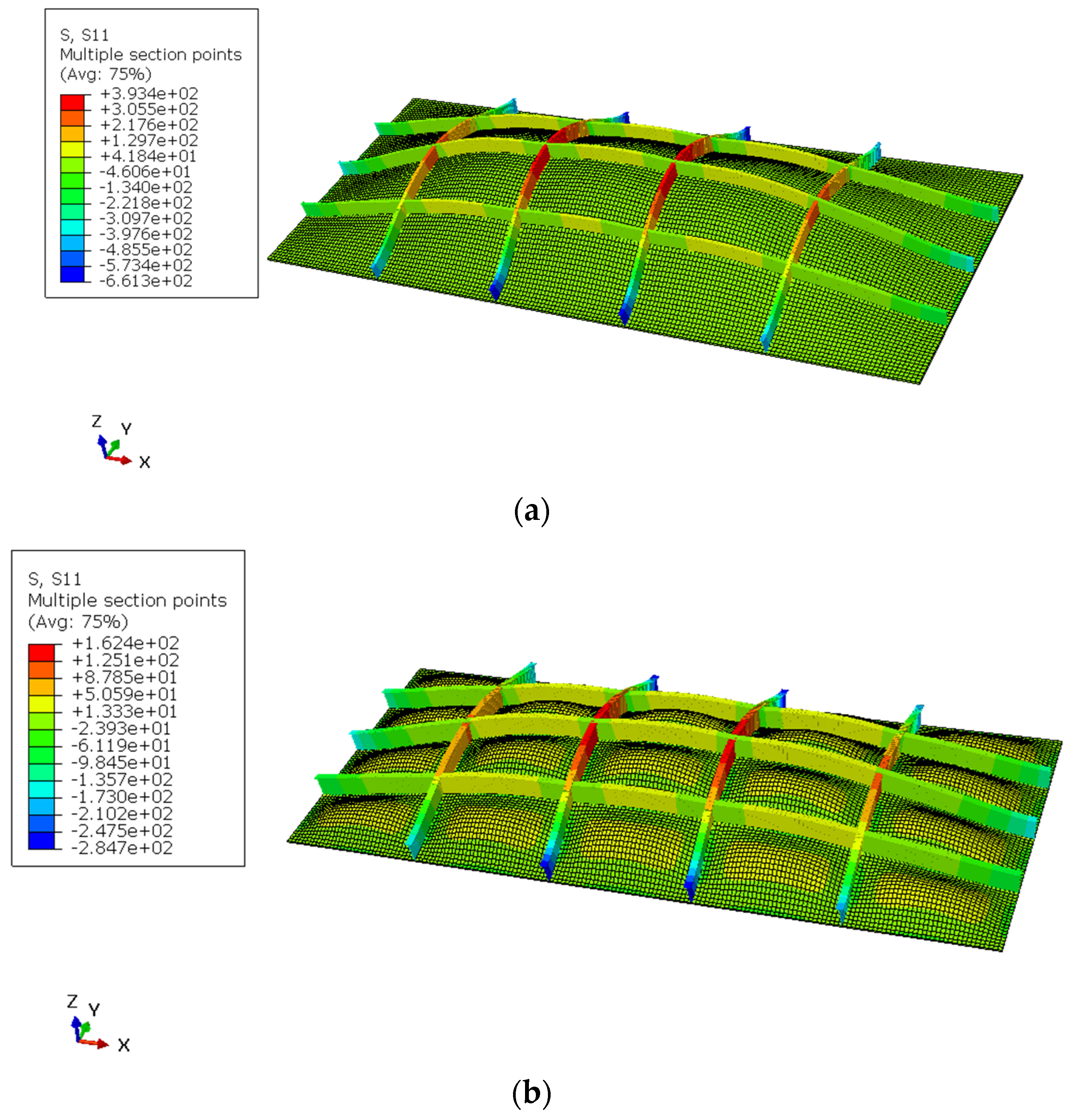
Figure 10 presents the normal bending stress along each stiffener direction for two different modeled cases. It is evident that the mid-stiffener attained a symmetric stress field along its span (between two neighboring transverse stiffeners). The effect of the model extent (number of longitudinal and transverse stiffeners) and peripheral supports do not influence the target stiffener considered for post-calculations.
3.3. Assessment of the Results
Following the respective finite element simulation for each case defined above, the maximum normal stress along the mid longitudinal stiffener, was retrieved and substituted in the following equation which sources from Equation (12)
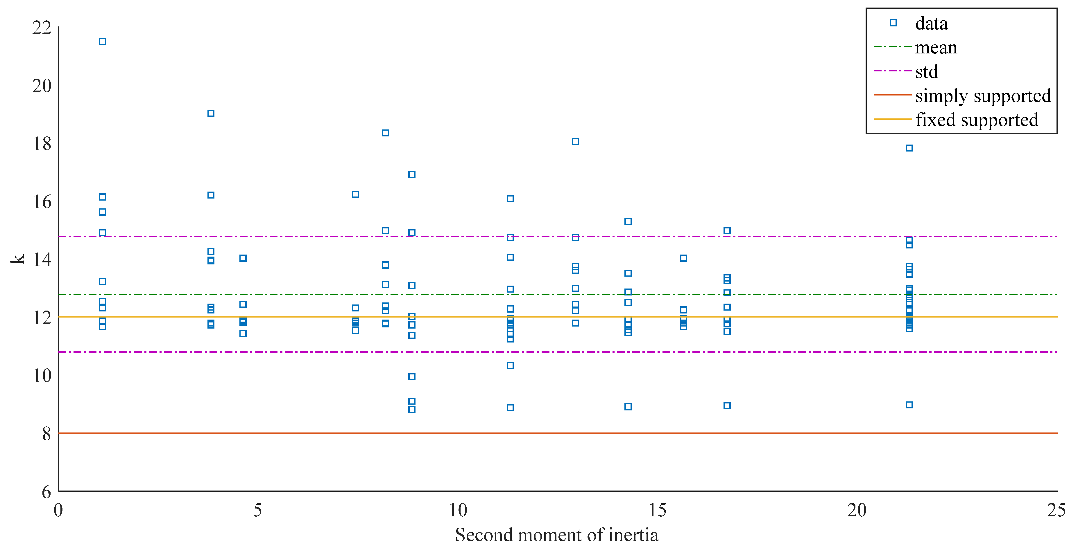
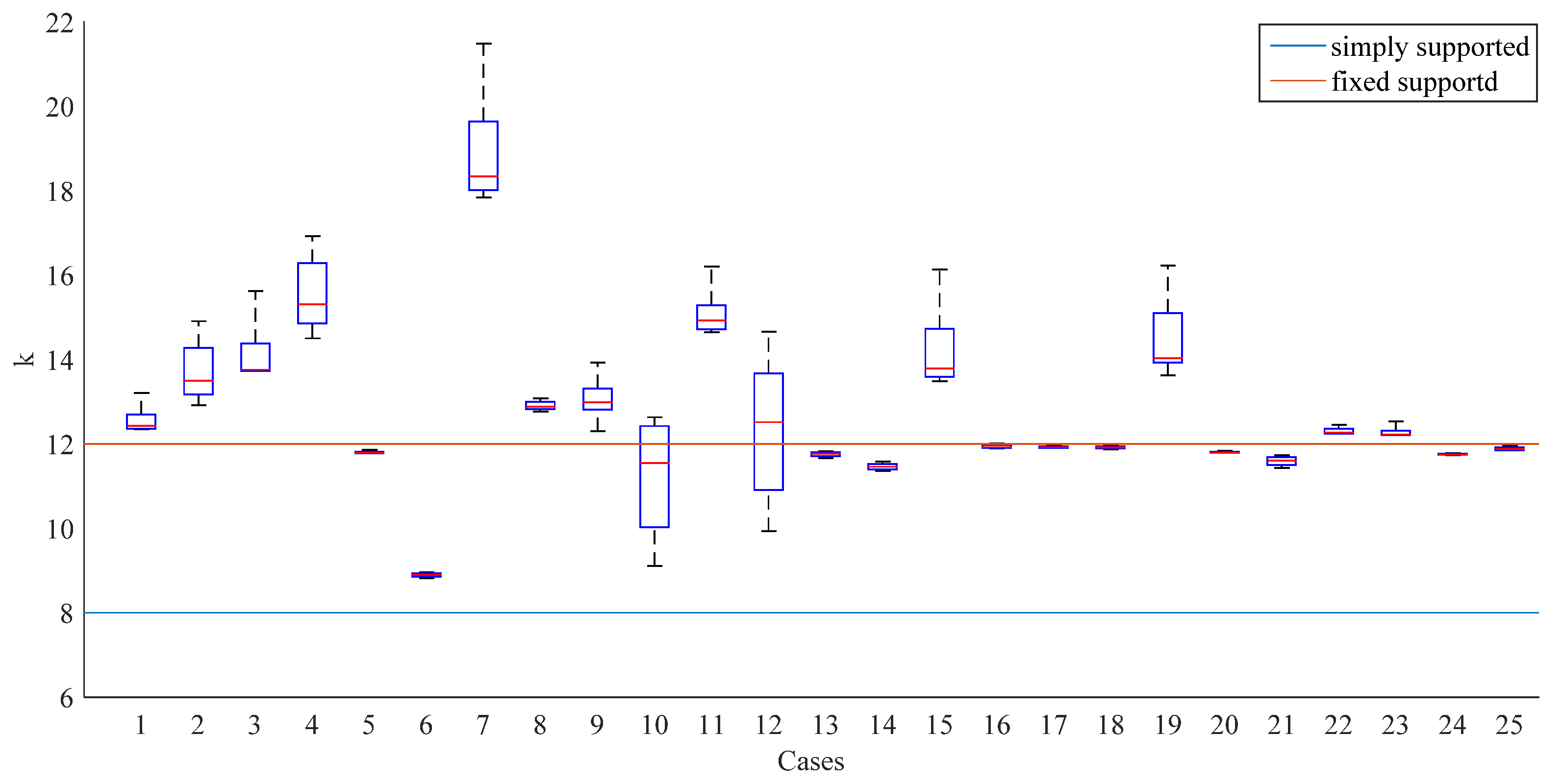
All obtained stiffness values k were plotted as a function of the corresponding second moment of inertia of the transverse stiffeners, as given in Table 4, in Figure 11. Most data are concentrated around k = 12 as the sample’s mean is 12.79 and the standard deviation is 1.99. As expected, none of the resultant k has a value smaller than 8 that corresponds to the case of a simply supported beam. It is noted that the theoretical values of k for simply and fixed supports are depicted with continuous lines.
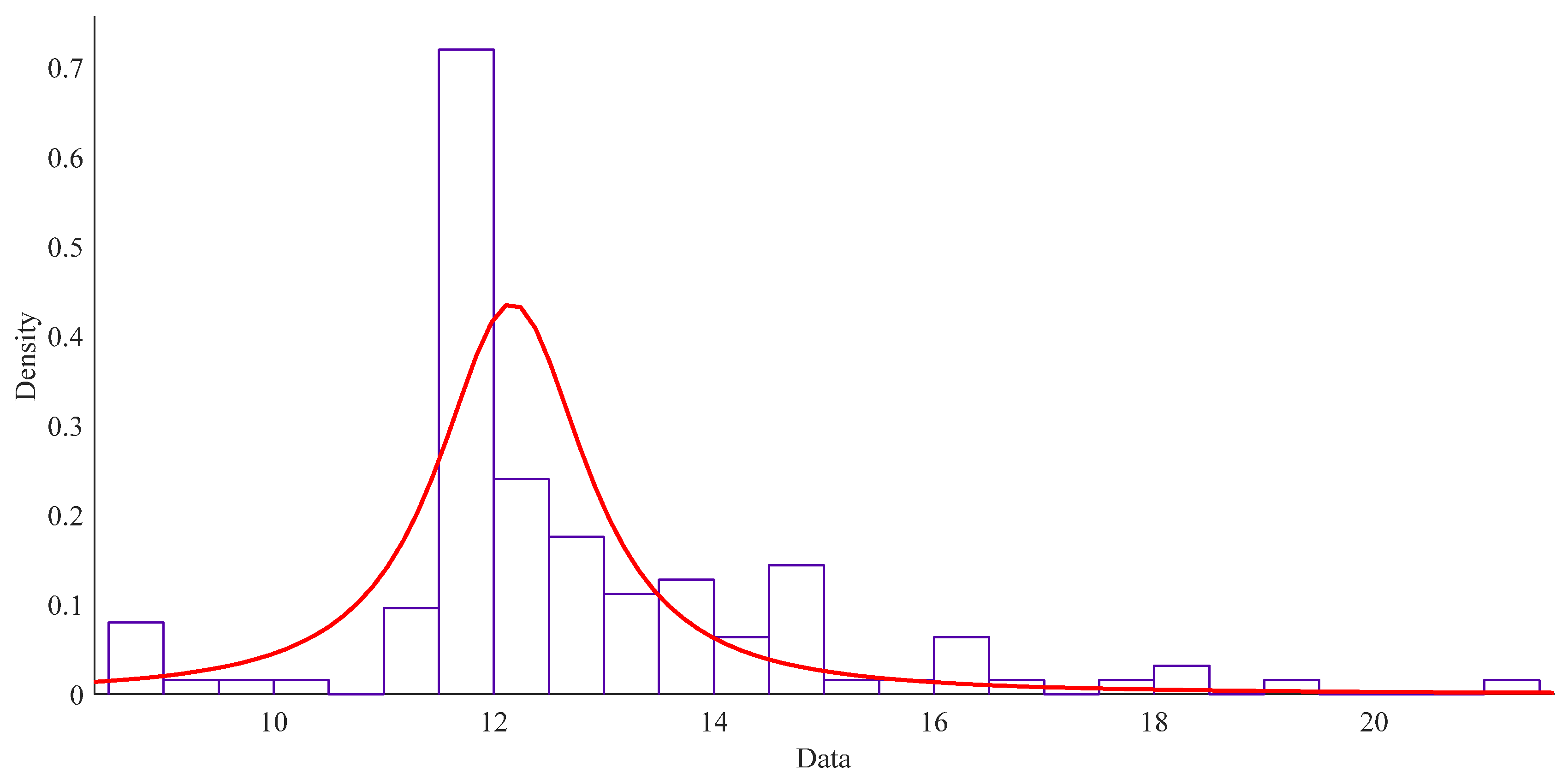
It is of interest to aggregate all data and build a histogram in order to perform descriptive statistics. Figure 12 presents the obtained statistical evaluations. It seems that the probability distribution of k can be approximated by the t location-scale probability density function (pdf) which has the following functional form:
where μ is the location parameter and is equal to 12.16, σ is the scale parameter and is equal to 0.77, ν is the shape parameter and is equal to 1.36 and is the gamma function given by:
The derived pdf may of course be used for assigning probabilities of occurrence to different values of k. For example, the corresponding probability that k receives values smaller than 8.0 is equal to 2.6%.
The effect of the second moment of inertia of transverse stiffeners to the value of k may be considered insignificant based on the general trend presented in the boxplot of Figure 13. For this reason, in Table 6, the coefficient k is given in relation with s, st, and I. For these three variables, within the limits that were mentioned before, coefficient k can be calculated using trilinear interpolation. This table may be used within the scantling process of cross-stiffened panels found in ship structures.
4. Conclusions
This study has worked toward two main objectives related to the secondary stresses developed in stiffened panels found in ship hull structures.
The first objective was to assess the effect of four different approaches used for incorporating the shear lag mechanism into the notion of the effective width for the case of one-way (single-bay) stiffened panels subjected to a uniform pressure load. Paik’s solution yields the minimum effective width of the attached plating, whereas Miller’s solution yields the maximum corresponding magnitude. Nevertheless, we have generated evidence based on FEA that the effect of either approach to the secondary stress field is statistically insignificant.
The second objective was to simplify the analysis of slender stiffeners of a cross-stiffened panel subjected to a uniform pressure as well as to reduce the problem to a single beam bending one and figure out the stiffness of the transverse stiffeners. As a general conclusion, this work has generated evidence that supports that a fully fixed condition (relative rotation not allowed) of the stiffener ends may be applied. A table that relates longitudinal and transverse spacing and moment of inertia with the corresponding k values is provided.
Although the presented research is concentrated at statically loaded stiffened panels, the methods could be used in time-dependent dynamic analysis and for inelastic buckling analysis and is an area that deserves exploring in future work.
Author Contributions
Conceptualization, K.N.A.; formal analysis, K.N.A.; investigation, E.L.P.; methodology, E.L.P. and K.N.A.; Validation, E.L.P.; writing—original draft, E.L.P. and K.N.A.; writing—review and editing, K.N.A. All authors have read and agreed to the published version of the manuscript.
Funding
This research received no external funding.
Institutional Review Board Statement
Not applicable.
Informed Consent Statement
Not applicable.
Conflicts of Interest
The authors declare no conflict of interest.
Abbreviations
| σ1,σx | normal bending stress |
| σmax | maximum normal bending stress |
| Mhg | hull-girder bending moment |
| Ihg | hull-girder moment of inertia |
| z | distance of material fibers from neutral axis |
| tp | plate thickness |
| αp | correction factor for the panel aspect ratio (αp = 1.2 − s/(2.1 st)) |
| P | applied pressure |
| χ | coefficient for plate scantling |
| Ca | permissible bending stress coefficient |
| REh | permissible material resistance |
| Zmin | minimum section modulus requirement |
| s | longitudinal stiffener spacing |
| lbdg | effective bending span |
| fbdg | coefficient based on effective bending span |
| Cs | coefficient |
| be | plate’s effective width (breadth) |
| Zact | actual section modulus |
| q(x,s) | shear flow |
| Q | first moment of inertia |
| I | second moment of inertia |
| V | shear force |
| τ(x,s) | shear stress |
| γ(x,s) | shear strain |
| G | shear modulus |
| E* | Effective Young’s modulus (taken as E or E/(1 − ν2)) |
| ν | Poisson’s ratio |
| e(s) | axial deformation |
| L | length of stiffened plate |
| fk (k) | propability distribution |
| Γ(∙) | gamma function |
| μ | location parameter |
| σ | scale parameter |
| ν | shape parameter |
Appendix A
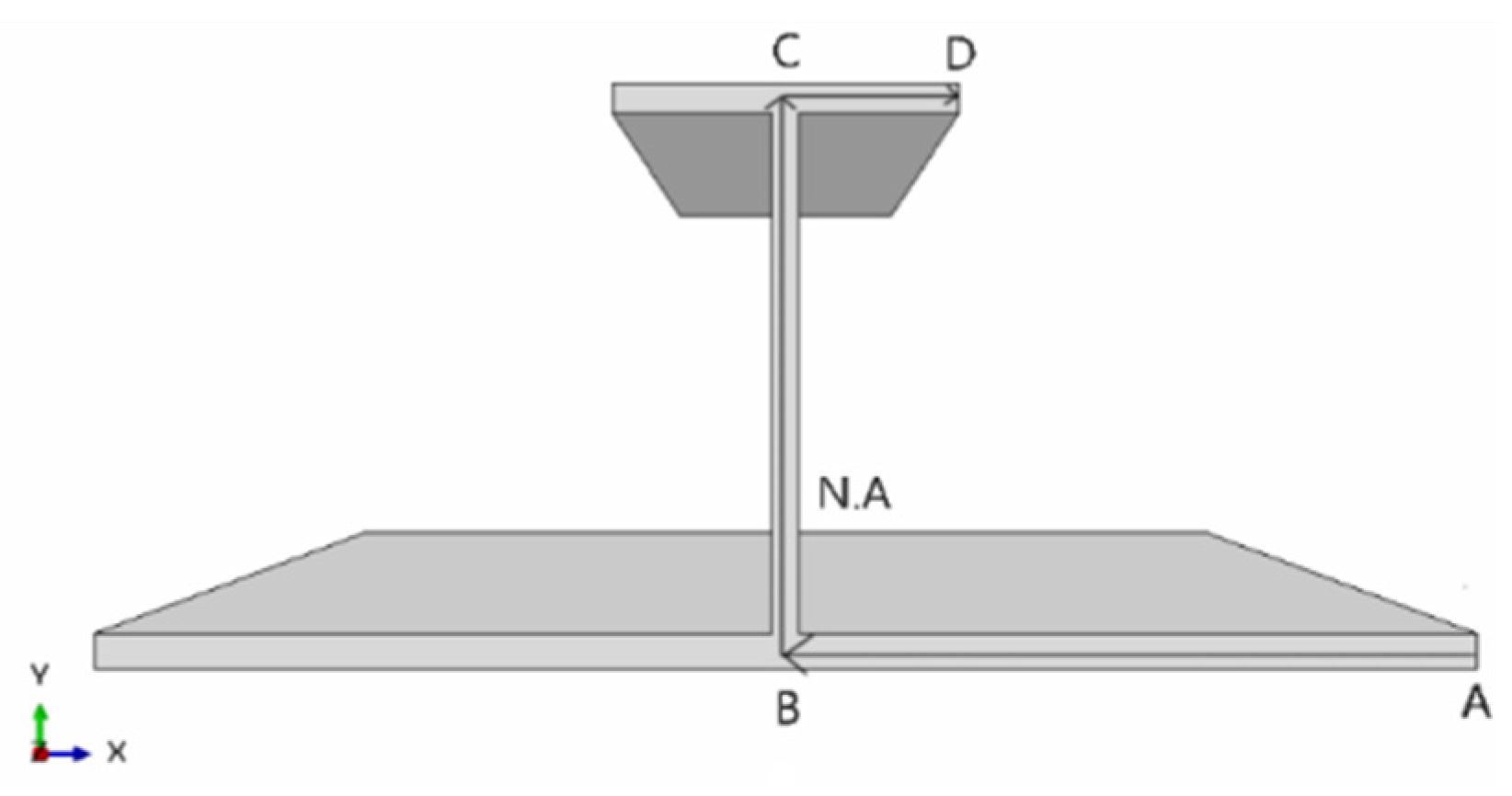
The appendix provides more details on Miller’s solution. Classical rules of mechanics are employed. The following step-by-step procedure undertaken in this work to derive the corresponding effective breadth. The formulation initiates with the calculation of the load effects, i.e., distribution of the bending moment and shear force along the length of the stiffener with the attached plating modeled by a beam, M(x) and V(x), respectively. The next step is to derive the shear flow at each section x, as q(x,s) based on the vertical shearing force; a task that is straightforward either for open or for closed cross-sectional profiles. The variable s is the local dimension that follows the predefined path ABCD shown in Figure A1. By calculating the first moment of inertia Q(s) per section element and the section’s second moment of inertia I, then q(x,s) is given as:
Figure A1.
Integration path for shear lag effect calculation.

The field of in-plane shear stresses, τ(x,s), can be calculated by dividing the shear flow over the thickness for each element of the cross-section, tel.(flange, web, attached plate):
The aforementioned shear stress field produces a corresponding in-plane shear strain γ(x,s), with a corresponding linear relation described by Hooke’s law:
where G is the shear modulus:
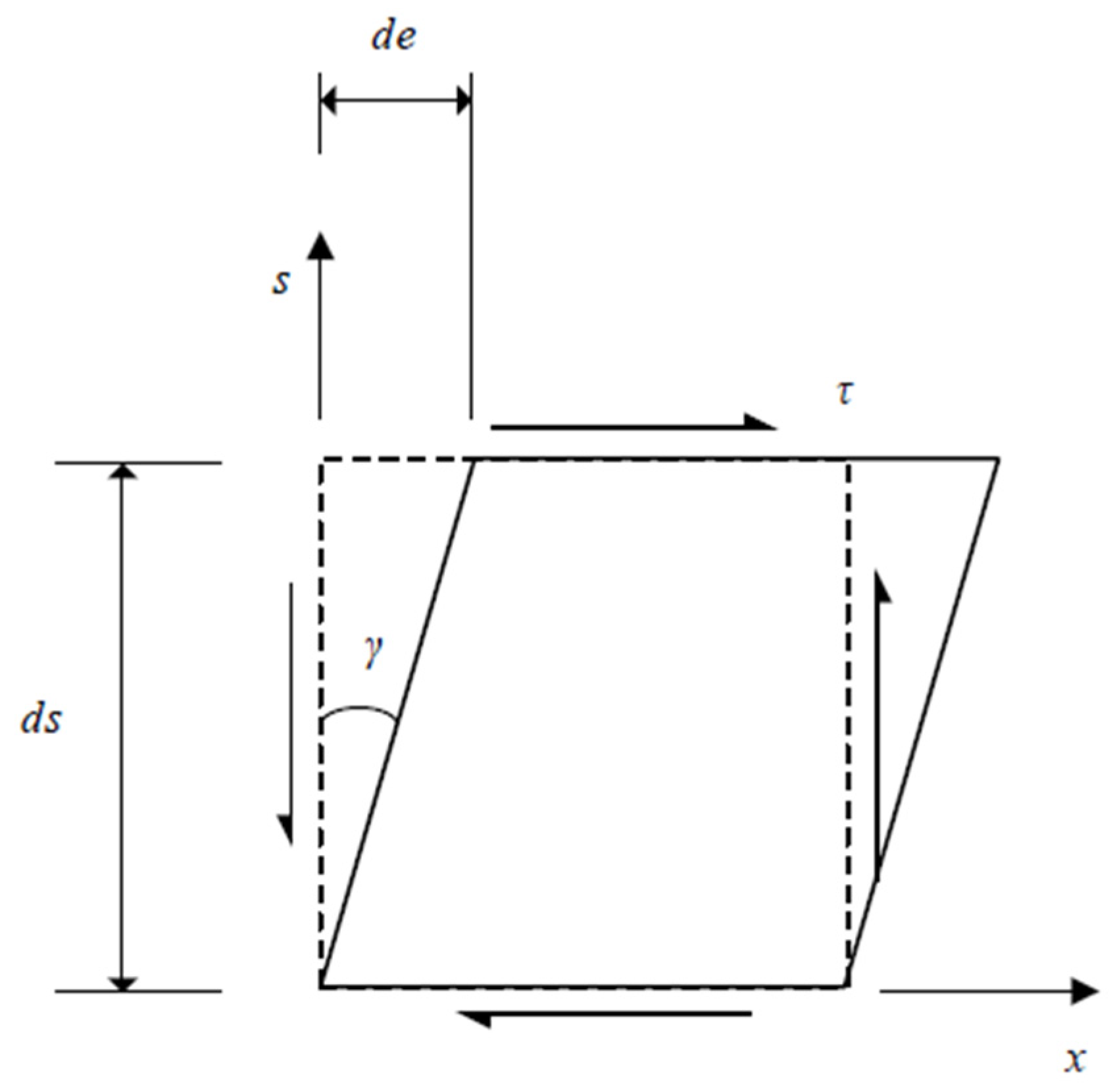
Equation (A3) denotes that shearing stresses produce a shearing deformation, which produces changes in right angles of infinitesimal planar elements dxds, as illustrated in Figure A2. These changes in the angles introduce changes in the length of material fibers as well, denoted as e, if not allowed to deform freely. In thin-walled composite sections under lateral loads, such deformation is constrained due to the relative stiffness of the involved elements. Hence axial deformations are of substantial importance and cannot be neglected. This is in fact the underlying mechanism of the shear lag problem that associates the shearing effect with the bending effect. On this foundation it is important to introduce a corresponding relation between kinematics as:
Figure A2.
Geometric definition of shear strain.

Equation (A5) is written for a given section x. By integrating over s, we can extract a relation for the axial deformation effect of shearing as:
By using Equation (A3), then Equation (A6) may be rewritten:
By differentiating Equation (A7) with respect to x, the axial strain due to shear lag effect, εshearlag, is introduced:
The corresponding axial stress, shearlag, may be given by Hooke’s law as:
where E* is either the uniaxial Young’s modulus, E, or the biaxial effective one, E/(1 − v2). Miller’s solution neglects the biaxial condition and considers only the 1D stress sate. For reasons of comprehensiveness, we have examined both approaches. By differentiating Equation (A7) with respect to x, Equation (A9) is rewritten as:
Substituting Equation (6) into Equation (A10), the following equation is generated:
By using Equation (A4), by assuming that the cross-section does not vary along the length and that from static equilibrium then Equation (A11) is rewritten as:
The preceding Equations (A11) and (A12) provide the key magnitudes for eventually deriving the effective breadth per case.
References
- Common Structural Rules (CSR). International Association of Classification Societies; Common Structural Rules: London, UK, 2021. [Google Scholar]
- Evans, H.R.; Kristek, V. A hand calculation of the shear lag effect in stiffened flange plates. J. Constr. Steel Res. 1984, 4, 117–134. [Google Scholar] [CrossRef]
- He, X.; Xiang, Y.; Chen, Z. Improved method for shear lag analysis of thin-walled box girders considering axial equilibrium and shear deformation. Thin-Walled Struct. 2020, 151, 106732. [Google Scholar] [CrossRef]
- Hughes, O.F.; Paik, J.K. Ship Structural Analysis and Design; The Society of Naval Architects and Marine Engineers: Alexandria, VA, USA, 2013. [Google Scholar]
- Jensen, S.S. On the shear coefficient in Timoshenko’s beam theory. J. Sound Vib. 1983, 87, 621–635. [Google Scholar] [CrossRef]
- Jiang, L.; Zhang, S.M. Effect of pressure on collapse behaviour of stiffened panel. In Development in Maritime Technology and Engineering; Guedes Soares & Santos: Lisbon, Portugal, 2021. [Google Scholar]
- Koo, K.K.; Wu, X.S. Shear lag analysis for thin-walled members by displacement method. Thin-Walled Struct. 1992, 13, 337–354. [Google Scholar] [CrossRef]
- Lee, C.K.; Wu, G.J. Shear lag analysis by the adaptive finite element method: 1. Analysis of simple plated structures. Thin-Walled Struct. 2000, 38, 285–309. [Google Scholar] [CrossRef]
- Li, S.; Benson, S.; Dow, R.S. A Timoshenko beam finite element formulation for thin-walled box girder considering inelastic buckling. Developments in the Analysis and Design of Marine Structures. In Proceedings of the 8th International Conference on Marine Structures (MARSTRUCT), Trondheim, Norway, 7–9 June 2021. [Google Scholar]
- Li, X.; Wan, S.; Zhang, Y.; Zhou, M.; Mo, Y. Beam finite element for thin-walled box girders considering shear lag and shear deformation effects. Eng. Struct. 2021, 233, 111867. [Google Scholar] [CrossRef]
- Miller, N.S. Shear Lag in Box Girders; Department of Naval Architecture and Ocean Engineering, University of Glasgow: Glasgow, UK, 1976. [Google Scholar]
- Paik, J.K. Ultimate Limit State Analysis and Design of Plated Structures, 2nd ed.; John Wiley & Sons Ltd.: London, UK, 2018. [Google Scholar]
- Prokic, A. New finite element for analysis of shear lag. Comput. Struct. 2002, 80, 1011–1024. [Google Scholar] [CrossRef]
- Schade, H.A. The effective breadth of stiffened plating under bending loads. Trans. SNAME 1951, 59, 403–420. [Google Scholar]
- Tahan, N.; Pavlovic, M.N.; Kotsovos, M.D. Shear-lag revisited: The use of single fourier series for determining the effective breadth in plated structures. Comput. Struct. 1997, 63, 759–767. [Google Scholar] [CrossRef]
- Tenchev, R.T. Shear lag in orthotropic beam flanges and plates with stiffeners. Int. J. Solids Struct. 1996, 33, 1317–1334. [Google Scholar] [CrossRef]
- Timoshenko, S.P.; Goodier, J.N. Theory of Elasticity; McGraw Hill: New York, NY, USA, 1951. [Google Scholar]
- Vedeler, G. DNV Rules (January 2013), Pt 3, Ch 1, Sec 3, C402. Available online: https://rules.dnv.com/docs/pdf/dnvpm/rulesship/2013-01/ts301.pdf (accessed on 6 January 2022).
Figure 1.
One-way (single-bay) stiffened panel (a) and cross-stiffened panel (b).

Figure 2.
Notion of the effective width, be, of the attached plating in stiffener bending. This figure shows a representative section of a stiffened plate with “Tee” profile stiffeners that have a specific spacing, s. The shear lag effect reduces the actual width and a corresponding static equivalent stress, σmax, is assumed.

Figure 3.
Miller’s solution (uniaxial E used in this graph, E* = E) for the representative sample of cases listed in Table 1.
Figure 3.
Miller’s solution (uniaxial E used in this graph, E* = E) for the representative sample of cases listed in Table 1.

Figure 4.
Comparison of effective width concept for the four considered cases.

Figure 5.
Modeled geometry with boundary conditions (all degrees of freedom in the boundary, i.e., connection with floors and girders are constrained) and uniformly distributed pressure load (with direction upwards) (a) and corresponding mesh (b) for the bottom stiffened panel.
Figure 5.
Modeled geometry with boundary conditions (all degrees of freedom in the boundary, i.e., connection with floors and girders are constrained) and uniformly distributed pressure load (with direction upwards) (a) and corresponding mesh (b) for the bottom stiffened panel.

Figure 6.
Longitudinal stress distribution (S22 in the model’s convention) over the bottom stiffened panel: left, full model; right, section cut.
Figure 6.
Longitudinal stress distribution (S22 in the model’s convention) over the bottom stiffened panel: left, full model; right, section cut.

Figure 7.
Longitudinal stress distribution (S22 in the model’s convention) over the topside wing tank stiffened panel: left, full model; right, section cut.
Figure 7.
Longitudinal stress distribution (S22 in the model’s convention) over the topside wing tank stiffened panel: left, full model; right, section cut.

Figure 8.
Simplified model that accounts for the rigidity of transverse stiffeners.

Figure 9.
Modeled geometry, boundary conditions (all degrees of freedom in the boundary, i.e., connection with transverse beams) and uniformly distributed pressure load (with direction upwards) (a) and corresponding mesh for the cross-stiffened panel (b). The stiffeners’ cross-sections are presented for rendering purposes.

Figure 10.
Stiffener bending normal stresses and deformation of a weak (a) and strong (b) stiffener system.
Figure 10.
Stiffener bending normal stresses and deformation of a weak (a) and strong (b) stiffener system.

Figure 11.
Results of k in relation tothe second moment of inertia of transverse stiffeners.

Figure 12.
Histogram of the k stiffness data and t location-scale distribution.

Figure 13.
Box plot for the value of k.


Table 1.
Dimensions of “Tee” profile stiffened panels.
| Stiffener Spacing (mm) | Thickness of Plate (mm) | Height of Web (mm) | Thickness of Web (mm) | Width of Flange (mm) | Thickness of Flange (mm) |
|---|---|---|---|---|---|
| 800 | 20 | 300 | 15 | 200 | 18 |
| 600 | 12 | 200 | 10 | 50 | 10 |
| 750 | 20 | 280 | 14 | 90 | 14 |
| 900 | 28 | 340 | 15 | 110 | 15 |
| 650 | 12 | 240 | 12 | 70 | 12 |
| 700 | 15 | 300 | 15 | 100 | 15 |
| 800 | 18 | 380 | 17 | 130 | 17 |
| 900 | 25 | 425 | 18 | 150 | 18 |
| 760 | 16 | 350 | 15 | 150 | 15 |
| 830 | 19 | 430 | 18 | 150 | 18 |
Table 2.
Assessment of the effective width solution with respect to the FEA maximum normal stress for the panel taken from the bottom area of the ship. In Miller’s solution the out of parenthesis corresponds at the uniaxial E* and within parenthesis at the biaxial E*.
Table 2.
Assessment of the effective width solution with respect to the FEA maximum normal stress for the panel taken from the bottom area of the ship. In Miller’s solution the out of parenthesis corresponds at the uniaxial E* and within parenthesis at the biaxial E*.
| Header | be/s | % Difference from FEA |
|---|---|---|
| Paik | 0.35 | 6.1 |
| Schade | 0.44 | 8.0 |
| CSR | 0.71 | 11.1 |
| Miller * | 0.96 (0.93) | 12.3 (12.1) |
* Lower Bound.
Table 3.
Assessment of the effective width solution with respect to the FEA maximum normal stress for the panel taken from the topside wing tank area of the ship. In Miller’s solution the out of parenthesis corresponds at the uniaxial E* and within parenthesis at the biaxial E*.
Table 3.
Assessment of the effective width solution with respect to the FEA maximum normal stress for the panel taken from the topside wing tank area of the ship. In Miller’s solution the out of parenthesis corresponds at the uniaxial E* and within parenthesis at the biaxial E*.
| Header | be/s | % Difference from FEA |
|---|---|---|
| Paik | 0.49 | 10.6 |
| Schade | 0.59 | 11.5 |
| CSR | 0.86 | 13.1 |
| Miller * (lower bound) | 0.98 (0.97) | 13.7 (13.4) |
* Lower Bound.
Table 4.
The test matrix of the variables of the model.
| st (mm) | s (mm) | tp (mm) | Is (mm × mm) |
|---|---|---|---|
| 1800 | 600 | 12 | 200 × 10 + 50 × 10 |
| 1800 | 600 | 12 | 340 × 15 + 110 × 15 |
| 1800 | 600 | 28 | 200 × 10 + 50 × 10 |
| 1800 | 600 | 28 | 340 × 15 + 110 × 15 |
| 5400 | 600 | 12 | 200 × 10 + 50 × 10 |
| 5400 | 600 | 12 | 340 × 15 + 110 × 15 |
| 5400 | 600 | 28 | 200 × 10 + 50 × 10 |
| 5400 | 600 | 28 | 340 × 15 + 110 × 15 |
| 1800 | 900 | 12 | 200 × 10 + 50 × 10 |
| 1800 | 900 | 12 | 340 × 15 + 110 × 15 |
| 1800 | 900 | 28 | 200 × 10 + 50 × 10 |
| 1800 | 900 | 28 | 340 × 15 + 110 × 15 |
| 5400 | 900 | 12 | 200 × 10 + 50 × 10 |
| 5400 | 900 | 12 | 340 × 15 + 110 × 15 |
| 5400 | 900 | 28 | 200 × 10 + 50 × 10 |
| 5400 | 900 | 28 | 340 × 15 + 110 × 15 |
| 3600 | 600 | 20 | 280 × 14 + 90 × 14 |
| 3600 | 900 | 20 | 280 × 14 + 90 × 14 |
| 1800 | 750 | 20 | 280 × 14 + 90 × 14 |
| 5400 | 750 | 20 | 280 × 14 + 90 × 14 |
| 3600 | 750 | 12 | 280 × 14 + 90 × 14 |
| 3600 | 750 | 28 | 280 × 14 + 90 × 14 |
| 3600 | 750 | 20 | 200 × 10 + 50 × 10 |
| 3600 | 750 | 20 | 340 × 15 + 110 × 15 |
| 3600 | 750 | 20 | 280 × 14 + 90 × 14 |
Table 5.
Longitudinal and transverse stiffener combinations considered.
| Longitudinal Stiffener 200 × 10 + 50 × 10 | Longitudinal Stiffener 280 × 14 + 90 × 10 | Longitudinal Stiffener 340 × 15 + 110 × 15 | |
|---|---|---|---|
| Transverse stiffeners | 200 × 10 + 50 × 10 | 280 × 14 + 90 × 14 | 340 × 15 + 110 × 15 |
| 270 × 13 + 85 × 13 | 320 × 15 + 105 × 15 | 360 × 16 + 120 × 16 | |
| 330 × 15 + 110 × 15 | 360 × 16 + 120 × 16 | 380 × 17 + 130 × 17 | |
| 375 × 16 + 130 × 16 | 390 × 17 + 140 × 17 | 400 × 17 + 140 × 17 | |
| 425 × 18 + 150 × 18 | 425 × 18 + 150 × 18 | 425 × 18 + 150 × 18 |
Table 6.
The coefficient k in relation with st, s and I.
| st (mm) | s (mm) | I (107 mm4) | K (-) |
|---|---|---|---|
| 1800 | 600 | 4.11 | 12.34 |
| 1800 | 600 | 25.62 | 12.92 |
| 1800 | 600 | 5.18 | 13.73 |
| 1800 | 600 | 33.85 | 14.5 |
| 5400 | 600 | 4.1 | 11.78 |
| 5400 | 600 | 25.62 | 8.82 |
| 5400 | 600 | 5.18 | 17.84 |
| 5400 | 600 | 33.85 | 12.77 |
| 1800 | 900 | 4.39 | 12.29 |
| 1800 | 900 | 28.85 | 9.11 |
| 1800 | 900 | 5.42 | 14.65 |
| 1800 | 900 | 36.54 | 9.93 |
| 5400 | 900 | 4.39 | 11.67 |
| 5400 | 900 | 28.85 | 11.37 |
| 5400 | 900 | 5.42 | 13.49 |
| 5400 | 900 | 36.54 | 11.89 |
| 3600 | 600 | 17.15 | 11.91 |
| 3600 | 900 | 18.56 | 11.88 |
| 1800 | 750 | 17.96 | 13.63 |
| 5400 | 750 | 17.96 | 11.78 |
| 3600 | 750 | 15.49 | 11.44 |
| 3600 | 750 | 19.72 | 12.24 |
| 3600 | 750 | 4.84 | 12.21 |
| 3600 | 750 | 32.12 | 11.73 |
| 3600 | 750 | 17.96 | 11.84 |
Publisher’s Note: MDPI stays neutral with regard to jurisdictional claims in published maps and institutional affiliations. |
© 2022 by the authors. Licensee MDPI, Basel, Switzerland. This article is an open access article distributed under the terms and conditions of the Creative Commons Attribution (CC BY) license (https://creativecommons.org/licenses/by/4.0/).
Share and Cite
MDPI and ACS Style
Platypodis, E.L.; Anyfantis, K.N. On the Modeling of Ship Stiffened Panels Subjected to Uniform Pressure Loads. Appl. Mech. 2022, 3, 125-143. https://0-doi-org.brum.beds.ac.uk/10.3390/applmech3010010
AMA Style
Platypodis EL, Anyfantis KN. On the Modeling of Ship Stiffened Panels Subjected to Uniform Pressure Loads. Applied Mechanics. 2022; 3(1):125-143. https://0-doi-org.brum.beds.ac.uk/10.3390/applmech3010010
Chicago/Turabian StylePlatypodis, Efstathios L., and Konstantinos N. Anyfantis. 2022. "On the Modeling of Ship Stiffened Panels Subjected to Uniform Pressure Loads" Applied Mechanics 3, no. 1: 125-143. https://0-doi-org.brum.beds.ac.uk/10.3390/applmech3010010