Mathematical Apparatus of Optimal Decision-Making Based on Vector Optimization

Far Eastern Federal University, 690068 Vladivostok, Russia
Appl. Syst. Innov. 2019, 2(4), 32; https://0-doi-org.brum.beds.ac.uk/10.3390/asi2040032
Submission received: 17 April 2019
/
Revised: 26 June 2019
/
Accepted: 29 June 2019
/
Published: 11 October 2019
(This article belongs to the Special Issue Fuzzy Decision Making and Soft Computing Applications)
Abstract
:We present a problem of “acceptance of an optimal solution” as a mathematical model in the form of a vector problem of mathematical programming. For the solution of such a class of problems, we show the theory of vector optimization as a mathematical apparatus of acceptance of optimal solutions. Methods of solution of vector problems are directed to problem solving with equivalent criteria and with the given priority of a criterion. Following our research, the analysis and problem definition of decision making under the conditions of certainty and uncertainty are presented. We show the transformation of a mathematical model under the conditions of uncertainty into a model under the conditions of certainty. We present problems of acceptance of an optimal solution under the conditions of uncertainty with data that are represented by up to four parameters, and also show geometrical interpretation of results of the decision. Each numerical example includes input data (requirement specification) for modeling, transformation of a mathematical model under the conditions of uncertainty into a model under the conditions of certainty, making optimal decisions with equivalent criteria (solving a numerical model), and, making an optimal decision with a given priority criterion.
1. Introduction
The problem of making an optimal decision that meets the modern achievements of science and technology is connected, firstly, with the release of high-quality products, and, secondly, with the solution of problems of social and economic human development. The decision making can be undertaken under the conditions of certainty (when the functional dependence of the purpose of the parameters of the studied object and systems is known) [1,2,3,4], and under the conditions of uncertainty (when there is not sufficient information on the functional dependence of the purpose of the parameters of the studied object and systems) [5,6,7,8]. The conditions of uncertainty are characterized by the fact that input data for decision-making, can be presented as random, fuzzy or incomplete data, [1,2,9,10]. Research on this problem of decision-making began with the work of Keeney and Raiffa [11]. Analyses of modern decision-making approaches (i.e., “simple” methods) are submitted in [6,12]. One of the areas of decision-making automation is associated with the creation of mathematical models and the adoption of an optimal solution based on them [12,13,14]. Currently, the most common mathematical apparatus for model-based decision making is vector optimization [6,12,14,15,16,17,18,19]. The purpose of this work is to build a mathematical model for an object or system of decision making in the form of a vector problem of mathematical programming. Vector optimization is considered as a mathematical apparatus of a solution to the problem of acceptance of an optimal solution.
For the realization of the goal of this work, the study considered and solved the following problems.
The construction of a mathematical model of the problem of finding an optimal solution in the form of a vector problem of mathematical programming has been shown previously [4,6,15,20]. In the current paper, the theory and a mathematical apparatus of problem solving using vector optimization are presented. The theory includes an axiomatic principle of optimality of the solution of vector problems. The mathematical apparatus of the solution of vector problems is intended for the solution of vector problems with equivalent criteria [6,13,21] and with the given priority of a criterion [15,20]. The research, analysis and problem definition of decision making under the conditions of certainty and uncertainty are conducted. The realization of a mathematical apparatus of vector optimization is presented for numerical problems of decision making with one, two, three and four parameters. The solution of the problem of decision making includes creation of a numerical model of an object in the form of a vector problem, the solution of a problem of decision making with equivalent criteria, and, the solution of a vector problem of decision making with a criterion priority.
2. Statement of a Problem: Creation of the Mathematical Model “Acceptance of an Optimal Solution”
As an “object for optimal decision-making,” we use a “technical system”. The problem of the choice of optimum parameters of technical (engineering) systems according to functional characteristics arises during the study, analysis, and design of technical systems, and is connected with quality production.
The problem includes the solution of the following tasks:
- Creation of a mathematical model, which defines the inter-relation of each functional characteristic from parameters of the technical system, i.e., it is formed from the vector problem of mathematical programming;
- Choice of methods of the decision: we suggest using the methods based on normalization of criteria and the principle of the guaranteed result with equivalent criteria and with the set criterion priority;
- Development of the software which realizes these methods;
The technical system depends on N, a set of design data: X = {x1, x2, …, xN}, where N is the number of parameters, each of which lies in the set limits:
where x, x, ∀j ∈ N are the minimum and maximum limits of change of the vector of parameters of the technical system.
The result of the functioning of the technical system is defined by a set К of technical characteristics of fk(X), k = which functionally depend on design data X = {xj, j = }, in total these represent a vector function: F(X) = (f1(X) f2(X) … fK (X))T.
The set of characteristics (criteria) is subdivided into two subsets K1 and K2: К = K1K2.
K1 is a subset of technical characteristics, the numerical values of which are desired to be as high as possible: fk(X) max, k = .
K2 is a subset of technical characteristics, the numerical values of which are desired to be as low as possible: fk(X) min, k = , K2 ≡ .
The mathematical model should consider, firstly, the purposes of the technical system which are represented by the characteristics of F(X), and, secondly, the Xmin ≤ X ≤ Xmax restrictions. The mathematical model of the technical system which solves in general a problem of the choice of the optimum design decision (a choice of optimum parameters) is presented in the form of a vector problem of mathematical programming.
where X is the vector of controlled variables (constructive parameters) in Equation (1), F(X) = {fk(X), k = } represents the vector criterion for each component of the characteristics of the technical system in Equation (2), which functionally depends on the vector of variables X, G(X) = (g1(X) g2(X) … gM(X))T represents a vector of the restrictions imposed on the functioning of the technical system, and M is a set of restrictions.
G(X) ≤ 0,
Restrictions are defined in terms of technological, physical or similar processes, and can be presented by functional restrictions, for example, f≤ fk(X) ≤ f, k = .
It is supposed that the fk(X), k = functions are differentiated and convex, gi(X), i = are continuous, and Equations (3)–(4) represent a non-empty set of admissible points of S restrictions, which can be represented as S = {X ∈ RN|G(X) ≤ 0, Xmin ≤ X ≤ Xmax} ≠ ø.
Criteria and restrictions in Equations (1)–(4) form the mathematical model of a technical system. It is required to find a vector of the X0 ∈ S parameters at which every component of the vector-functions F1(X) = {fk(X), k = } accepts the greatest possible value, and vector-functions F2(X) = {fk(X), k = } are accepted by the minimum value.
For a substantial class of technical systems which can be represented by the vector problem of Equations (1)–(4), it is possible to refer to their large number of applications in various fields, such as electro-engineering [23], airspace [10,13], metallurgical (choice of optimal structure of material), and chemical [24].
In this article, the technical system is considered to be static. However, technical systems can be considered to be dynamic [23], using differential-difference methods of transformation, conducted for a small discrete period Δt ∈ T.
3. Theory. Axioms, the Principle of Optimality and Methods for Solving Vector Problems of Mathematical Programming
The theory of vector optimization includes theoretical foundations (axioms) and methods of the solution of vector problems with equivalent criteria and with the given criterion priority. The theory is a basis of mathematical apparatus of modeling of an “object for optimal decision-making”, which allows selection of any point from a set of points that is Pareto optimal, and shows why the selection is optimal.
We have presented, first, axioms and methods of the solution of problems of vector optimization with equivalent criteria (Section 3.1) and, second, the specified priority criteria (Section 3.2).
3.1. Vector Optimization with Equivalent Criteria
3.1.1. Axioms and the Principle of Optimality of Vector Optimization with Equivalent Criteria
Definition 1.
(Definition of the relative assessment of criteria).
In the vector problem of Equations (1)–(4), definitions are as follows: λk(X) = , ∀k ∈ K is the relative estimate of a point X ∈ S kth criterion, fk(X) is the kth criterion at the point X ∈ S, f is the value of the kth criterion at the point of optimum X, obtained in the vector problem of Equations (1)–(4) of the individual kth criterion, f is the worst value of the kth criterion (anti-optimum) at the point X (superscript 0) on the admissible set S in Equations (1)–(4), at the task at max (3), (5), (6), the value of f is the lowest value of the kth criterion, f = fk(X) ∀k ∈ K1 and the task min f is the greatest, f = fk(X) ∀k ∈ K2. The relative estimate of λk(X), ∀k ∈ K is firstly measured in relative units and, secondly, the relative assessment of λk(X) ∀k ∈ K on the admissible set is changed from zero at a point of X: ∀k ∈ K λk(X) = 0, to the unit at the point of an optimum of X:∀k ∈ K, λk(X) = 1, i.e.,: ∀k ∈ K, 0 ≤ λk(X) ≤ 1, X ∈ S. This allows the comparison of the criteria, measured in relative units, by joint optimization.
Axiom 1.
(About equality and equivalence of criteria at an admissible point of vector problems of mathematical programming)
In vector problems of mathematical programming two criteria with the indexes k ∈ K, q ∈ K shall be considered as equal at point X ∈ S if relative estimates of the kth and qth criterion are equal at this point, i.e., λk(X) = λq(X), k, q ∈ K.
We will consider criteria equivalent in vector problems of mathematical programming at a point X ∈ S if, when comparing the numerical size of relative estimates of λk(X), k = , for each criterion of fk(X), k = , and, respectively, relative estimates of λk(X), conditions are not imposed about the priorities of criteria.
Definition 2.
(Definition of a minimum level among all relative estimates of criteria).
The relative level λ in a vector problem represents the lower assessment of a point of X ∈ S among all relative estimates of λk(X), k = :
The lower level for the performance of the condition of Equation (5) at an admissible point of X ∈ S is defined as:
Equations (5) and (6) are interconnected. They serve as a transition from Equation (6) of the definition of a minimum to the restrictions of Equation (5), and vice versa.
The level λ allows the union of all criteria in a vector problem with one numerical characteristic of λ, made over certain operations, thereby carrying out these operations over all criteria measured in relative units. The level λ functionally depends on the X ∈ S variable, by changing X, we can change the lower level, λ. From here we will formulate the rules of searching for the optimum decision.
Definition 3.
(The principle of optimality with equivalent criteria).
The vector problem of mathematical programming with equivalent criteria is solved if the point of X0 ∈ S and a maximum level of λ0 (the top index optimum) among all relative estimates is found such that:
Using the interrelation of Equations (5) and (6), we will transform the maximine problem of Equation (7) into an extreme problem:
We can call the resulting problem of Equations (8) and (9) the λ-problem.
The λ-problem of Equations (8) and (9) has (N + 1) dimensions. As a consequence, the solution of the λ-problem represents an optimum vector of X° ∈ RN+1, where (N + 1) is a component which has the essence of the value of λ0, i.e., X0 = {x, x, ..., x, x}, thus x = λ0, and (N + 1) is a component of a vector of X0 selected in view of its specificity.
The obtained pair of {λ0, X0} = X0 characterizes the optimum solution of the λ-problem and according to the vector problem of mathematical programming in Equations (1)–(4) with equivalent criteria, can be solved on the basis of normalization of criteria and the principle of the guaranteed result. In the optimum solution of X0 = {X0, λ0}, X0 is an optimal point and λ0 is a maximum level.
An important result of the algorithm for solving the vector problems of Equations (1)–(4) with equivalent criteria is the following theorem.
Theorem 1.
(The theorem of the two most contradictory criteria in the vector problem of mathematical programming with equivalent criteria).
In convex vector problems of mathematical programming with equivalent criteria that are solved on the basis of normalization of criteria and the principle of the guaranteed result, for an optimum point of X0 = {λ0, X0}, two criteria are denoted by their indexes q ∈ K, p ∈ K (which in a sense are the most contradictory of the criteria k = ), for which an equality is carried out:
and other criteria are defined by inequalities:
λ0 = λq(X0) = λp(X0), q, p ∈ K, X ∈ S,
λ0 ≤ λk(X0) ∀k ∈ K, q ≠ p ≠ k.
3.1.2. Mathematical Algorithm of the Solution of a Vector Problem with Equivalent Criteria
To solve the vector problems of mathematical programming of Equations (1)–(4), the methods based on axioms of the normalization of criteria and the principle of the guaranteed result [12,21] are offered. Methods follow from Axiom 1 and the principle of optimality (Definition 3). We will present this as a number of steps as follows:
The method of the solution of the vector problem of Equations (1)–(4) with equivalent criteria is presented in the form of the sequence of steps [25].
Step 1. The problem of Equations (1)–(4) is solved separately for each criterion, i.e., for ∀k ∈ K1 is solved at the maximum, and for ∀k ∈ K2 is solved at a minimum. As a result of the decision, we obtain X, an optimum point by the corresponding criterion, k = ; f = fk(X), the kth criterion size at this point, k = .
Step 2. We define the worst value of each criterion on S: f, k = . For the problem of Equations (1)–(4) for each criterion of k = , a minimum is solved as: f = min fk(X), G(X) ≤ B, X ≥ 0, k = .
In addition, for Equations (1)–(4) for each criterion, a maximum is solved as: f = max fk(X), G(X) ≤ B, X ≥ 0, k = .
As a result of the decision, we obtain X = {xj, j = }, an optimum point by the corresponding criterion, k = ; f = fk(X), the kth criterion size at the point, X, k = .
Step 3. For the system analysis of a set of Pareto optimal points, for this purpose optimum points of X = {X, k = }, are defined as sizes of criterion functions of F(X*) and relative estimates λ(X), λk(X) = , ∀k ∈ K:
As a whole, for the problem ∀k ∈ К the relative assessment of λk(X), k = lies within 0 ≤ λk(X) ≤ 1, ∀k ∈ К.
Step 4. Creation of the λ-problem.
Creation of the λ-problem is carried out in two stages: initially build the maximine problem of optimization with the normalized criteria, which at the second stage will be transformed into the standard problem of mathematical programming called the λ-problem.
For the construction of the maximine problem of optimization we use Definition 2, relative level ∀X ∈ S, λ = λk(X).
The bottom λ level is maximized on X ∈ S, as a result, we obtain a maximine problem of optimization with the normalized criteria:
At the second stage we transform the problem of Equation (13) into a standard problem of mathematical programming:
where the vector of unknowns of X has the dimension N + 1: X = {λ, x1, …, xN}.
λ0 = max λ, → λ0 = max λ,
G(X) ≤ B, X ≥ 0, → G(X) ≤ B, X ≥ 0,
Step 5. Solution of the λ-problem.
The λ-problem of Equations (14)–(16) is a standard problem of convex programming for which decision standard methods are used.
As a result of the solution of the λ-problem, the following are obtained:
- X0 = {λ0, X0}, an optimum point,
- fk(X0), k = , values of the criteria at this point,
- λk(X0) = , k = , sizes of the relative estimates,
λ0, the maximum relative estimates which represent the maximum bottom level for all relative estimates of λk(X0), or the guaranteed result in relative units. λ0 guarantees that all relative estimates of λk(X°) are equal λ0: λk(X0) ≥ λ0, k = or λ0 ≤ λk(X0), k = , X0 ∈ S, and according to Theorem 1 [12,21], the point of X0 = {λ0, x1, …, xN} is Pareto optimal.
3.1.3. Implementation of the Decision using the Example of a Vector Problem of Linear Programming with Equivalent Criteria
The use of the vector problem of Equations (1)–(4) for decision making is carried out in four stages: statement of the problem, construction of the mathematical model, software development for solving the vector problem, and, solution of the vector problem.
These stages are carried out on the example of a model of an economic system presented by a vector problem of linear programming with equivalent criteria.
Stage 1. Statement of the problem.
As an economic system, a model of the production schedule of an enterprise is considered.
It is given that the company, which produces heterogeneous products of four types, N = 4, uses resources of three types, M = 3, in production: labor (various specialties), material (different types of materials), power (equipment: welding, turning, etc.).
The technological matrix of production is presented in Table 1. It also indicates the potential of the enterprise for each type of the resource bi, i = , as well as income and profit from the sale of a unit of each type of product.
It is required to make the production schedule of the enterprise, which includes indicators according to the nomenclature (by types of products) and on a volume basis, i.e., how many products of the corresponding type should be made by the enterprise so that income and profit can be realized as shown above. Construction and solution of the mathematical model follow.
Stage 2. Construction of a mathematical model.
As variables, we take the volume of products that the company produces: X = {x1, …, xN}, N = 4. We express target orientation of the production schedule by means of a vector problem of linear programming (VPLP) which will take the form:
opt F(X) = {max f1(X) = (4.0x1 + 5.0x2 + 9.0x3 + 11.0x4),
max f2(X) = (2x1 + 10x2 + 6x3 + 20x4)},
with restrictions x1 + x2 + x3 + x4 ≤ 15,
7x1 + 5x2 + 3x3 + 2x4 ≤ 120,
3x1 + 5x2 +10x3 +15x4 ≤ 100, x1 ≥ 0, x2 ≥ 0, x3 ≥ 0, x4 ≥ 0.
In this VPLP the following is formulated: it is required to find the non-negative solution of x1, …, x4 in the system of inequalities at which the f1(X) and f2(X) functions obtain maximum values.
Stage 3. The software engineering of the solution of the VPLP.
The “Solution of a Vector Problem of Linear Programming” program is presented in the annex to this section.
Stage 4. Solution of a vector problem of linear programming.
We show the solution of a problem of linear programming in the MATLAB system according to an algorithm of the solution of the VPLP on the basis of normalization of criteria and the principle of the guaranteed result. At first input data are prepared (the italicized font indicates the text of the program in the MATLAB system). The vector target function in the form of a matrix is formed:
disp (‘Solution of a vector problem of the linear programming’)
cvec = [ −4.0 −5.0 −9.0 −11.0, % Sales volume
−2. −10. −6. −20.] % profit Volume
a = [1.0 1.0 1.0 1.0,
7.0 5.0 3.0 2.0,
3.0 5.0 10.0 15.0], % matrix of linear restrictions
b= [15. 120. 100] % the vector containing restrictions (bi)
Aeq = [], beq = [] % restriction like equality
X0 = [0. 0. 0. 0.], % a vector of variables
The algorithm of the solution of VPLP is represented as a sequence of steps.
Step 1. A decision on each criterion.
The decision on the first criterion of the VPLP: [x1,f1] = linprog(cvec(1,:),a,b,Aeq,beq,lb,ub)
Decision on the first criterion: = x1 = {x1 = 7.14, x2 = x4 = 0, x3 = 7.85}, = f1 = −99.286.
Decision on the second criterion: = {x1 = 0, x2 = 12.5, x3 = 0, x4 = 2.5}, = f2 = 175.
Step 2. The worst point of an optimum is determined for each criterion (anti-optimum) by multiplication of criterion by a minus unit. For the decisions on the first and second criterion:
= x1min = {x1 = 0, …, x4 = 0}, = f1min = 0.
= x2min = {x1 = 0, …, x4 = 0}, = f2min = 0.
Step 3. The system analysis of the criteria in the VPLP is undertaken (i.e., the system of two criteria at optimum points is analyzed). For this purpose, optimum points of , are defined sizes of criterion functions and relative estimates of: F(X*) = , λ(X*) = , λ(X*) = , k = , F(X*) = = , λ(X*) = = .
Step 4. The λ-problem is constructed as: λ0 = max λ,
with restrictions λ − (f1(X) − )/( − ) ≤ 0, λ − (f2(X) − )/( − ) ≤ 0, G(X) ≤ B, X ≥ 0.
Substituting numerical data, we obtain:
λ0 = max λ,
with restrictions: λ − (4.0x1 + 5.0x2 + 9.0x3 + 11.0x4 − )/( − ) ≤ 0,
λ − (2x1 +10x2 + 6x3 + 20x4 − )/( − ) ≤ 0,
x1 + x2 + x3 + x4 ≤ 15,
7x1 + 5x2 + 3x3 + 2x4 ≤ 120,
3x1 + 5x2 + 10x3 + 15x4 ≤ 100,
x1 ≥ 0, x2 ≥ 0, x3 ≥ 0, x4 ≥ 0.
Step 5. Solution of the λ-problem.
Results of the solution of the λ-problem:
X0 = {x1 = 0.9217914, x2 = 0.0, x3 = 11.73964, x4 = 1.520722, x5 = 1.739639} - optimum values of variables,
λ0 = 0.9218, the optimum value of the criterion function
We execute a check, at an optimum point of X0 we determine sizes of criterion functions of F(X0) = {fk(X0), k = }, relative estimates of λ(X0) = {λk(X0), k = }.
As a result of the decision we obtain: fX0 = [f1(X0) = 91.52, f2(X0) = 161.3],
λ1(X0) = 0. 9218, λ2(X0) = 0.9218, i.e., λ0 ≤ λk(X0), k = 1,2.
These results show that at point X0 both criteria in the relative units reached λ0 = 0.92 from the optimum sizes. Any increase in one of the criteria of this level leads to a decrease in the other criterion, i.e., the point X0 is Pareto optimal.
Here we present the text of the program in the MATLAB system.
The application.
%Vector linear programming problem, 2 criteria
% Author: Машунин Юрий Константинович - Mashunin Yury. K.
%The program is designed for the training and research, for the commercial purposes please contact:
disp(Vector linear programming problem - 2 criteria’)
disp(‘ opt F(X) = {max f1(X) = (4.0x1 + 5.0x2 +9.0x3 + 11.0x4), ‘)
disp(‘ max f2(X) = (2x1 + 10x2 + 6x3 + 20x4),’)
disp(‘ x1 + x2 + x3 + x4 <= 15,’)
disp(‘7x1 +5x2 + 3x3 + 2x4 <= 120,’)
disp(‘3x1 +5x2 +10x3 +15x4 <= 100, x1 >= 0,..., x42 >= 0 ’)
cvec = [-4.0 -5.0 -9.0 -11.0.; -2. -10. -6. -20.];
disp(‘‘Step 0. Input data of the vector problem’)
cvec = [-4.0 -5.0 -9.0 -11.0; -2. -10. -6. -20.];
a = [1. 1. 1. 1.; 7. 5. 3. 2.; 3. 5. 10. 15.];
b = [15. 120. 100.]; Aeq = []; beq = []; x0 = [0. 0. 0. 0.];
disp(‘Step 1.The solution for each criterion is the best’)
[x1,f1] = linprog(cvec(1,:),a,b,Aeq,beq,x0)
[x2,f2] = linprog(cvec(2,:),a,b,Aeq,beq,x0)
disp(‘Step 2. Solution by criterion-best-worst’)
[x1min,f1min] = linprog(-1*cvec(1,:),a,b,Aeq,beq,x0)
[x2min,f2min] = linprog(-1*cvec(2,:),a,b,Aeq,beq,x0)
disp(‘Step 3. System analysis of the results of the decision’)
d1 = -f1- f1min; d2 = -f2- f2min;
f = [cvec(1,:)*x1 cvec(2,:)*x1; cvec(1,:)*x2 cvec(2,:)*x2]
L = [(-f(1,1) - f1min)/d1 (-f(1,2) - f2min)/d2;
(-f(2,1) − f1min)/d1 (-f(2,2) - f2min)/d2]
disp(‘Step 4. Solution of L-problem’);
cvec0 = [-1. 0. 0. 0. 0.];
a0 = [1. -4.0/d1 -5.0/d1 -9.0/d1 -11.0/d1;
1. -2./d2 -10./d2 -6./d2 -20./d2;
0. 1. 1. 1. 1.;
0. 7. 5. 3. 2.;
0. 3. 5. 10. 15.];
b0 = [- f1min/d1 − f2min)/d2 15. 120. 100.]; x00 = [0. 0. 0. 0. 0.];
[X0,L0] = linprog(cvec0,a0,b0,Aeq,beq,x00)
fX0 = [cvec(1,:)*X0(2:5) cvec(2,:)*X0(2:5)]
LX0 = [(-fX0(1)- f1min)/ d1 (-fX0(2) - f2min)/d2]
3.2. Vector Optimization with a Criterion Priority
3.2.1. Axioms and the Principle of Optimality of Vector Optimization with a Criterion Priority
For development of methods of the solution of problems of vector optimization with a priority of criterion we use definitions as follows:
- priority of one criterion of vector problems, with a criterion priority over other criteria,
- numerical expression of a priority,
- the set priority of a criterion,
- the lower (minimum) level from all criteria with a priority of one of them,
- a subset of points with priority by criterion (Axiom 2),
Definition 4.
(About the priority of one criterion over the other).
The criterion of q ∈ K in the vector problem of Equations (12) and (13) in a point of X ∈ S has priority over other criteria of k = , and the relative estimate of λq(X) by this criterion is greater than or equal to relative estimates of λk(X) of other criteria, i.e.:
and a strict priority for at least one criterion of t∈K,
Introduction of the definition of a priority of criterion in the vector problem of Equations (1)–(4) executed the redefinition of the early concept of a priority. Earlier the intuitive concept of the importance of this criterion was outlined, now this “importance” is defined as a mathematical concept: the higher the relative estimate of the qth criterion compared to others, the more it is important (i.e., more priority), and the highest priority at a point of an optimum is X, ∀q ∈ K.
From the definition of a priority of criterion of q ∈ K in the vector problem of Equations (1)–(4), it follows that it is possible to reveal a set of points Sq ⊂ S that is characterized by λq(X) ≥ λk(X), ∀k ≠ q, ∀X ∈ Sq. However, the answer to whether a criterion of q ∈ K at a point of the set Sq has more priority than others remains open. For clarification of this question, we define a communication coefficient between a couple of relative estimates of q and k that, in total, represent a vector: Pq(X) = {p(X)|k = }, q ∈ K ∀X ∈ Sq.
Definition 5.
(About numerical expression of a priority of one criterion over another).
In the vector problem of Equations (12) and (13), with priority of the qth criterion over other criteria of k = , for ∀X ∈ Sq, and a vector of Pq(X) which shows how many times a relative estimate of λq(X), q ∈ K, is more than other relative estimates of λk(X), k = , we define a numerical expression of the priority of the qth criterion over other criteria of k = as:
Definition 6.
(About the set numerical expression of a priority of one criterion over another).
In the vector problem of Equations (1)–(4) with a priority of criterion of q ∈ K for ∀X ∈ S, vector Pq = {p, k = } is considered to be set by the person making decisions (i.e., decision-maker) if everyone is set a component of this vector. Set by the decision-maker, component p, from the point of view of the decision-maker, shows how many times a relative estimate of λk(X), k = is greater than other relative estimates of λk(X), k = . The vector of p, k = is the numerical expression of the priority of the qth criterion over other criteria of k = :
The vector problem of Equations (1)–(4), in which the priority of any criteria is set, is called a vector problem with the set priority of criterion. The problem of a task of a vector of priorities arises when it is necessary to determine the point X0 ∈ S by the set vector of priorities. In the comparison of relative estimates with a priority of criterion of q ∈ K, as well as in a task with equivalent criteria, we define the additional numerical characteristic of λ which we call the level.
Definition 7.
(About the lower level among all relative estimates with a criterion priority).
The λ level is the lowest among all relative estimates with a priority of criterion of q∈ such that:
The lower level for the performance of the condition in Equation (19) is defined as:
Equations (19) and (20) are interconnected and serve as a further transition from the operation of the definition of the minimum to restrictions, and vice versa. In Section 3.1, we gave the definition of a Pareto optimal point X0 ∈ S with equivalent criteria. Considering this definition as an initial one, we will construct a number of the axioms dividing an admissible set of S into, first, a subset of Pareto optimal points S0, and, secondly, a subset of points Sq ⊂ S, q ∈ K, with priority for the qth criterion.
Axiom 2.
(About a subset of points, priority by criterion).
In the vector problem of Equations (12)–(13), the subset of points Sq ⊂ S is called the area of priority of criterion of q ∈ K over other criteria, if ∀X ∈ Sq ∀k∈K λq(X) ≥ λk(X), q ≠ k.
This definition extends to a set of Pareto optimal points S0 that is given by the following definition.
Axiom 2a.
(About a subset of points, priority by criterion, on Pareto’s great number in a vector problem). In a vector problem of mathematical programming the subset of points S ⊂ S0 ⊂ S is called the area of a priority of criterion of q∈K over other criteria, if ∀X ∈ S ∀k ∈ K λq(X) ≥ λk(X), q ≠ k.
In the following we provide explanations.
Axiom 2 and 2а allow the breaking of the vector problem in Equations (1)–(4) into an admissible set of points S, including a subset of Pareto optimal points, S0 ⊂ S, and subsets:
One subset of points S’ ∈ S where criteria are equivalent, and a subset of points of S’ crossed with a subset of points S°, allocated to a subset of Pareto optimal points at equivalent criteria S00 = S’ ∩ S0. As will be shown further, this consists of one point of X0 ∈ S, i.e., X0 = S00 = S’ ∩ S0, S’ ∈ S, S0 ∈ S.
“K” subsets of points where each criterion of q = has a priority over other criteria of k = , q ≠ k, and thus breaks, first, sets of all admissible points S, into subsets Sq ⊂ S, q = and, second, a set of Pareto optimal points, S0, into subsets S ⊂ S0 ⊂ S, q = . This yields: S’U() = S0, S ⊂S0 ⊂ S, q = .
We note that the subset of points S, on the one hand, is included in the area (a subset of points) of priority of criterion of q∈K over other criteria: S⊂ Sq ⊂ S, and, on the other, in a subset of Pareto optimal points: S ⊂ S0 ⊂ S.
Axiom 2 and the numerical expression of priority of criterion (Definition 5) allow the identification of each admissible point of X∈S (by means of vector Pq(X) = {p(X) = λq(X)/λk(X), k = }), to form and choose:
- a subset of points by priority criterion Sq, which is included in a set of points S, ∀q ∈ K X ∈ Sq ⊂ S, (such a subset of points can be used in problems of clustering, but is beyond this article);
- a subset of points by priority criterion S, which is included in a set of Pareto optimal points S°, ∀q∈K, X∈S ⊂ S0.
Thus, full identification of all points in the vector problem of Equations (12) and (13) is executed in sequence as:
| Set of admissible points of X∈S → | Subset of points, optimum across Pareto, X∈S0 ⊂S → | Subset of points, optimum across Pareto X∈S ⊂ S0 ⊂ S → | Separate point of а ∀X∈S X∈S ⊂ S0 ⊂ S |
This is the most important result which allows the output of the principle of optimality and to construct methods of a choice of any point of Pareto’s great number.
Definition 8.
(Principle of optimality 2. The solution of a vector problem with the set criterion priority).
The vector problem of Equations (12) and (13) with the set priority of the qth criterion of p, k = is considered solved if the point X0 and maximum level λ0 among all relative estimates is found such that:
Using the interrelation of Equations (19) and (20), we can transform the maximine problem of Equation (33) into an extreme problem of the form:
We call Equations (22) and (23) the λ-problem with a priority of the qth criterion.
The solution of the λ-problem is the point X0 = {X0, λ0} This is also the result of the solution of the vector problem of Equations (1)–(4) with the set priority of the criterion, solved on the basis of normalization of criteria and the principle of the guaranteed result.
In the optimum solution X0 = {X0, λ0}, X0, an optimum point, and λ0, the maximum bottom level, the point of X0 and the λ0 level correspond to restrictions of Equation (15), which can be written as: λ0 ≤ pλk(X0), k = .
These restrictions are the basis of an assessment of the correctness of the results of a decision in practical vector problems of optimization.
From Definitions 1 and 2, “Principles of optimality”, follows the opportunity to formulate the concept of the operation “opt”.
Definition 9.
(Mathematical operation “opt”).
In the vector problem of Equations (1)–(4), in which “max” and “min” are part of the criteria, the mathematical operation “opt” consists of the definition of a point X0 and the maximum λ0 bottom level to which all criteria measured in relative units are lifted:
i.e., all criteria of λk(X0), k = are equal to or greater than the maximum level of λ0 (therefore λ0 is also called the guaranteed result).
Theorem 2.
(The theorem of the most inconsistent criteria in a vector problem with the set priority).
If in the convex vector problem of mathematical programming of Equations (1)–(4) the priority of the qth criterion of p, k = , ∀q ∈ K over other criteria is set, at a point of an optimum X0 ∈ S obtained on the basis of normalization of criteria and the principle of guaranteed result, there will always be two criteria with the indexes r ∈ K, t ∈ K, for which the following strict equality holds:
and other criteria are defined by inequalities:
Criteria with the indexes r∈K, t∈K for which the equality of Equation (38) holds are called the most inconsistent.
Proof. Similar to Theorem 2 [25].
We note that in Equations (25) and (26), the indexes of criteria r, t ∈ K can coincide with the q ∈ K index.
Consequence of Theorem 1, about equality of an optimum level and relative estimates in a vector problem with two criteria with a priority of one of them.
In a convex vector problem of mathematical programming with two equivalent criteria, solved on the basis of normalization of criteria and the principle of the guaranteed result, at an optimum point Xo equality is always carried out at a priority of the first criterion over the second:
and at a priority of the second criterion over the first:
λ0 = p(X0)λ1(X0) = λ2(X0), X0 ∈ S, where p(X0) = λ2(X0)/λ1(X0).
3.2.2. Mathematical Method of the Solution of a Vector Problem with Criterion Priority
(Method of the decision in problems of vector optimization with a criterion priority) [25].
Step 1. We solve a vector problem with equivalent criteria. The algorithm of the decision is presented in Section 3.1.2. As a result of the decision we obtain:
- optimum points by each criterion separately X, k = and sizes of criterion functions in these points of f = fk(X), k = , which represent the boundary of a set of Pareto optimal points,
- anti-optimum points by each criterion of X = {xj, j = } and the worst unchangeable part of each criterion of f = fk(X), k = ,
- X0 = {λ0, X0}, an optimum point, as a result of the solution of VPMP at equivalent criteria, i.e., the result of the solution of a maximine problem and the λ-problem constructed on its basis,
- λ0, the maximum relative assessment which is the maximum lower level for all relative estimates of λk(X0), or the guaranteed result in relative units, λ0 guarantees that all relative estimates of λk(X0) are equal to or greater than λ0:
The person making the decision carries out the analysis of the results of the solution of the vector problem with equivalent criteria. If the received results satisfy the decision maker, then the process concludes, otherwise subsequent calculations are performed.
In addition, we calculate:
- in each point X, k = we determine sizes of all criteria of q = :{fq(X), q = }, k = , and relative estimatesλ(X) = {λq(X), q = , k = }, λk(X) = , ∀k ∈ K:
Matrices of criteria of F(X*) and relative estimates of λ(X*) show the sizes of each criterion of k = upon transition from one optimum point X, k∈K to another X, q∈K, i.e., on the border of a great number of Pareto.
- at an optimum point at equivalent criteria X0 we calculate sizes of criteria and relative estimates:which satisfy the inequality of Equation (28). In other points X∈S0, in relative units the criteria of λ = λk(X) are always less than λ0, given the λ-problem of Equations (22) and (23).
This information is also a basis for further study of the structure of a great number of Pareto.
Step 2. Choice of priority criterion of q ∈ K.
From theory (see Theorem 1) it is known that at an optimum point X0 there are always two most inconsistent criteria, q ∈ K and v ∈ K, for which in relative units an exact equality holds: λ0 = λq(X0) = λp(X0), q, v ∈ K, X ∈ S. Others are subject to inequalities: λ0 ≤ λk(X0) ∀k ∈ K, q ≠ v ≠ k.
As a rule, the criterion which the decision-maker would like to improve is part of this couple, and such a criterion is called a priority criterion, which we designate q ∈ K.
Step 3. Numerical limits of the change of the size of a priority of criterion q ∈ K are defined.
For priority criterion q ∈ K from the matrix of Equation (29) we define the numerical limits of the change of the size of criterion:
where fq(X) derives from the matrix of Equation (29) F(X*), all criteria showing sizes measured in physical units, fq(X0) from Equation (30), and,
where λq(X) derives from the matrix λ(X*), all criteria showing sizes measured in relative units (we note that λq(X) = 1), λq(X0) from Equation (29).
As a rule, Equations (31) and (32) are given for the display of the analysis.
Step 4. Choice of the size of priority criterion (decision-making).
The person making the decision carries out the analysis of the results of calculations of Equation (42) and from the inequality of Equation (31) chooses the numerical size fq of the criterion of q∈K:
For the chosen size of the criterion of fq it is necessary to define a vector of unknown Xo. For this purpose, we carry out the subsequent calculations.
Step 5. Calculation of a relative assessment.
For the chosen size of the priority criterion of fq the relative assessment is calculated as:
which upon transition from point X0 to X, according to Equation (32), lies in the limits: λq(X0) ≤ λq ≤ λq(X) = 1.
Step 6. Calculation of the coefficient of linear approximation.
Assuming a linear nature of the change of criterion of fq(X) in Equation (31) and according to the relative assessment of λq(X) in Equation (32), using standard methods of linear approximation we calculate the proportionality coefficient between λq(X°), λq, which we call ρ:
Step 7. Calculation of coordinates of priority criterion with the size fq.
In accordance with Equation (33), the coordinates of the Xq priority criterion point lie within the following limits: X0 ≤ Xq ≤ X, q ∈ K. Assuming a linear nature of change of the vector Xq = {x, …, x} we determine coordinates of a point of priority criterion with the size fq with the relative assessment of Equation (32):
where X0 = {x, …, x}, X = {x(1), …, x(N)}.
Step 8. Calculation of the main indicators of a point xq.
For the obtained point xq, we calculate:
- all criteria in physical units fk(xq) = {fk(xq), k = },
- all relative estimates of criteria λq = {λ, k = }, λk(xq) = , k = ,
- the vector of priorities Pq = {p = , k = },
- the maximum relative assessment λoq = min (pλk(xq), k = ).
Any point from Pareto’s set X = {λ, X}∈So can be similarly calculated.
Analysis of results. The calculated size of criterion fq(X), q∈K is usually not equal to the set fq. The error of the choice of Δfq = |fq(X) − fq| is defined by the error of linear approximation.
4. Research, Analysis, and Formulation of the Problem of Decision-Making with Uncertain Data
4.1. Investigation of the Model of the “Object for Making an Optimal Decision” under Certainty and Uncertainty
4.1.1. Characteristics of Certainty and Uncertainty
Building a mathematical model of an “object or system for making an optimal decision” (Equations (1)–(4)) is possible, under conditions of certainty and uncertainty, which happen often. Conditions of certainty are characterized by the fact that the functional dependence of each criterion fk, k = (1) and the constraints G(3) on the system parameters xj, j = , is known [6,12,22].
To build a mathematical model of a system under certainty, studies of the physical processes occurring in the system are conducted. At the creation of a mathematical model of such processes, fundamental laws of physics are used, for example, models of magnetic and temperature profiles, and laws of conservation of energy and movement. A complete list of all functional characteristics of technical systems and parameters on which these characteristics depend is formed. Their verbal description is given. The technical and information interrelationships of all components of a technical system is established, i.e., the structure is under construction. At this stage, the problem of the choice of the best structure of a technical system (a problem of structural optimization) is solved [4,23].
As a result of the conducted research, the functional interrelationship of a set of characteristics of F1(X), F2(X) and restrictions of G(X) from parameters X has to be constructed.
Conditions of uncertainty are characterized by that there is no sufficient information on the functional dependence of each characteristic and the restrictions on the parameters [8,9,12,20].
At the same time, there are two problems associated with decision making.
The first problem is characterized by the fact that only data for some of the indicators are known (such a task is presented in the following section, see Equation (37)). The second problem is that data on some set of parameters, as well as relevant data on some set of characteristics (criteria), of a problem are known (38).
Both problems arise when carrying out pilot studies based on the principle of “ input-output”. On the basis of the conducted pilot studies, there is a problem with the adoption of the acceptable decision. We present the analysis of these problems and decision making on their basis in the following sections.
Thus, under conditions of certainty the function fk(X), k ∈ K is known, for the infinite set of parameters there is a corresponding infinite set of estimates of the function (criterion). Conversely, under conditions of uncertainty, only a finite set of parameters and the corresponding set of function (criterion) estimates are known, the smaller the set of parameters, the higher the uncertainty.
4.1.2. Investigation of Condition of Uncertainty
Conditions of uncertainty are considered in two aspects. The first relates to a lack of sufficient information. This is the uncertainty associated with the variety of characteristics (criteria) of the object under study.
This aspect is defined by the fact that there is not sufficient information on the functional dependence of the characteristic f and restrictions g from parameters X of the studied object. In this case, input data characterizing the object are presented as:
- (a)
- random data,
- (b)
- fuzzy data, or
- (c)
- incomplete data, which are usually obtained from experimental data.
For options (a) and (b), input data have to be transformed into option (c), and are presented in table form: 1 column—parameter size, 2 columns—characteristic size. The methodology of the transformation of random and fuzzy data into tabular form is presented in the magazine “Fuzzy Decision Making and Soft Computing Applications”. Tabular (experimental) data, using regression analysis, will be transformed into the f(X) function, i.e., in terms of certainty.
In the future, only variant c) is considered in this work, and its transformations by regression methods into certainty conditions, i.e., into the function f(X).
The second aspect of decision-making uncertainty is related to the fact that an object is characterized by many characteristics: f1(X), …, fK(X). The set of characteristics K is divided into two subsets K1 and K2. The subset of characteristics K1 in a numerical value is desired to be as high as possible (maximum), and the subset of characteristics K2 is desired to be as low as possible (minimum). Below it will be shown that the decision-making problem with a set of characteristics is reduced to a vector problem of mathematical programming, the solution of which is presented in Section 3.
4.2. Conceptual Problem Definition of Decision Making under the Conditions of Uncertainty
Initially, from a general view the conceptual problem definition of decision making was presented in work of R. L. Keeney and H. Raiffa [11], according to which we denote аi, i = , for the admissible decision-making alternatives, and A = (a1 a2 … aM) for the vector of the set of admissible alternatives.
We match each alternative a ∈ A to K numerical indices (criteria) f1(a), …, fK(a) that characterize the system. We can assume that this set of indices maps each alternative onto the point of the K-dimensional space of outcomes (consequences) of decisions made, F(a) = (f1(a) f2(a) … fK(a))T. We use the same symbol fk(a) both for the criterion and for the function that performs the estimation with respect to this criterion. Note that we cannot directly compare the variables fv(a) and fk(a), v ≠ k at any point F(a) of the K-dimensional space of consequences since it would most likely have no sense because these criteria are generally measured in different units. Using these data, we can state the decision-making problem.
The decision maker is to choose an alternative а ∈ A to obtain the most suitable result, i.e., F(a) min.
This definition means that the required estimating function should reduce the vector F(a) to a scalar preference or “value” criterion. In other words, it is equivalent to setting a scalar function V given the space of consequences and possessing the following property:
where the symbol means “no less preferable than” [24]. We call the function V(F(a)) the value function. The name of this function in other publications may vary from an order value function to a preference function to a value function. Thus, the decision maker is to choose а ∈ A such that V(F(a)) is maximized. The value function allows an indirect comparison of the importance of certain values of various criteria of the system. Thus, the matrix F(a) of admissible outcomes of alternatives takes the form:
where fi j = fi (ai) and all alternatives in it are represented by the vector of indices F(a). For the sake of definiteness and without loss of generality, we assume that the first criterion (any criterion can be the first) is arranged in increasing (decreasing) order, with the alternatives re-numbered i = .
Problem 1 (Equation (37)) implies that the decision maker is to choose the alternative a0 ∈ A such that it will yield the “most suitable (optimal) result” [24].
For an engineering system, we can represent each alternative ai by the N-dimensional vector Xi = {xij, j = }, i = } of its parameters, and its outcomes by the K-dimensional vector criterion {f1(Xi), …, fK(Xi), i = }. Taking this into account, the matrix of outcomes (Equation (37)) takes the form:
Problem 2 (Equation (38)) for decision makers consists of the choice of the set of design data X0 = {xij, j = }, i = } that would allow the optimal result [24].
4.3. The Analysis of Modern Methods of Decision Making to the Experimental Data
At present, the problems of Equations (37) and (38) are solved by a number of “simple” methods based on special criteria, such as Wald, Savage, Hurwitz, and Bayes–Laplace criteria, which provide the basis for decision making.
The Wald criterion of maximizing the minimal component helps make the optimal decision that ensures the maximal gain among minimal ones, .
The Savage minimal risk criterion chooses the optimal strategy so that the value of the risk is minimal among maximal values of risks over the columns, . The value of the risk is chosen from the minimal difference between the decision that yields maximal profit , k = , and the current value , = () − , with their set being the matrix of risks .
The Hurwitz criterion helps choose the strategy that lies somewhere between absolutely pessimistic and optimistic (i.e., the most considerable risk):
where α is the pessimistic coefficient chosen in the interval 0 ≤ α ≤ 1.
The Bayes–Laplace criterion takes into account each possible consequence of all decision options, given their probabilities .
All these and other methods are widely described in publications on decision making [11]. All have certain drawbacks. For instance, if we analyze the Wald maximin criterion, we can see that by the problem’s hypothesis all criteria are in different units. Hence, the first step, which is to choose the minimal component = , is quite reasonable. However, all , k = , are measured in different units, therefore the second step, which is to maximize the minimal component , is pointless. Although it brings us slightly closer to a solution, the criteria measurement scale fails to solve the problem since the chosen criteria scales are judgmental.
We believe that to solve the problem of Equations (37) and (38), we need to form a measure that would allow the evaluation of any decision to be made, including the optimal one. In other words, we need to construct an axiom that shows, based on the set of K criteria, what makes one alternative better than the other. In turn, the axiom can help derive a principle that determines whether the chosen alternative is optimal. The optimality principle should become the basis for the constructive methods of choosing optimal decisions. We propose such an approach for the vector mathematical programming problem that is essentially close to the decision-making problem of Equations (37) and (38).
4.4. Transforming the Decision-Making Problem into Vector Problem
We compare the decision-making problem (DMP) of Equations (37) and (38) with the vector problem mathematical programming (VPMP). Table 2 shows the comparison.
The first, second and third rows of Table 2 show that all three problems have the common objective of “making the best (optimal) decision”. Both types of decision-making problems (row 4) have some uncertainty, functional dependences of criteria and restrictions on the problem’s parameters are not known. At present, many mathematical methods of regression analysis are implemented in software (such as MATLAB) that allow using some set of initial data (as in Equations (37) and (38)) to construct the functional dependences fk(X), . For this reason, we use regression methods, including multiple regression, to construct criteria and restrictions in decision-making problems of both types (row 5) [26]. Combining criteria and restrictions, we represent decision-making problems of both types as a vector mathematical programming problem (row 6).
We perform these transformations. We use methods of regression analysis for the problem of Equation (37) and multiple regression for the problem of Equation (38) to transform each kth column of the matrix into the criterion function fk(X). We combine them in the vector function F(X): max F1(X) = {fk(X), } in Equation (1), and, min F2(X) = {fk(X), } in Equation (2). The inequalities:
where = , = , are the minimal and maximal values of each function, and the parameters bounded by minimal and maximal values of each of them serve as functional restrictions (Equation (3)). The result is a VPMP (Equations (1)–(4)) and uses the same methods based on normalizing criteria and maximin principles as for the ES model under complete certainty to solve it for tantamount criteria.
5. Statement and Optimal Decision Making with Experimental Data in Problems with One Parameter
We use a particular example to illustrate the decision-making problem of the first type (Equation (37)) and the choice of the optimal decision. We also show the proposed method is independent of the form of the sought extremum of partial criteria.
5.1. Problem Definition of Decision Making of the First Type
The problem definition is carried out by the designer of the system on experimental data.
It is given that the system is defined by one parameter X = {x}, a vector of (operated) variables. The experimental data for the task of decision making are provided in Table 3.
The system comprises one parameter {x} and four characteristics (criteria):
used to make a choice. Taken together, they constitute a decision-making problem of the first type.
The requirement is to make the best (optimal) decision given the experimental data available.
5.2. The Solution of the Problem
We find the optimal solution in two stages.
Stage 1. We transform the decision-making problem into a VPMP.
Step 1. We prepare the initial data in Table 2 in the form of the matrix I (Equation (38)). These watch points are shown in Figure 1, using MATLAB operators:
xlabel(′X′); ylabel(′Y′); hold on; plot(I(:,1),I(:,2)/10,′k.′);
plot(I(:,1)I(:,3),′go′); plot(I(:,1),I(:,4),′bp′); plot(I(:,1)I(:,5)*10,′r*′).
For the sake of visualization, the order of the first criterion is decreased by one while the order of the fourth criterion is increased by one.
Step 2. Using a method of the smallest square deviations [12], we calculate the coefficients of the approximating polynomial of the second degree:
An approximation is carried out in the MATLAB system using the polyfit function (X, Y, N) where X is a vector of tabular values (nodes), and Y represents preset values of assessment.
Limits of the change of parameter x of the lower and top scale in Figure 1 are set. In the MATLAB system, this is presented as x = −600.:100.:19000.
We calculate the first criterion by means of the function: c1=polyfit(I(:,1),I(:,2)/10,2). The result is c1(1) = –3.1937 × 10⁻⁶, c1(2) = 0.1947, c1(3) = 365.1, which corresponds to the polynomial of the second degree:
f1(x) = –3.1937 × 10−6 x2 + 0.1947x + 365.1.
We calculate the values of the polynomial y5 = polyval(c1,x) and show it on a graph using plot(x,y5,′k-′), hold on.
Similarly, the rest of the criteria are:
f2(x) = 9.467 × 10−10 x3 − 2.7968 × 10−5 x2 + 0.1090 x + 1949.2,
f3(x) = 1.0174 × 10−5 x2 − 0.1707x + 1737.4,
f4(x) = 1.6458 × 10−7 x2 − 0.01309x + 247.83.
All the resulting points and functions are also shown in Figure 1.
Step 3. We form and solve the VPMP. Using the results of the previous stage, we represent the decision making problem as the VPMP of Equations (1)–(4) with the vector criterion F(x) = (−f1(x) − f2(x) f3(x) − f4(x))T and restrictions 630 ≤ x ≤ 18,810:
Opt F(X) = {maxF1(X) = {maxf1(X), maxf2(X), maxf4(X)},
minF2(X) = {minf3X)},
Stage 2. We solve the VPMP of Equations (44)–(46) similarly to that shown in Section 2.
Step 1. We solve the problem of Equations (44)–(46) for each criterion separately. Since each is a unimodal function, we use the function [x,f] = fminbnd(c,a,b) to find its minimum or maximum on the segment (Equation (46)). Here, c, a, b are the input parameters, c is the given function, a and b are the beginning and the end of the interval, respectively, and x and f are the output parameters (the optimum point and the value of the objective function at the optimum, respectively). It takes the form:
for the first criterion. We thus derive the optimum point with respect to the first criterion x = 18,810 and the value of the criterion at this point = f1(x) = −28,969. Similarly, we have x = 2192.8, = f2(x) = −2063.7, x = 630.0, = f4(x) = −239.65, x = 8389.0, = f3(x) = 1021.4 for other criteria.
[x1max,f1max]=fminbnd(′−(3.1937 × 10⁻⁵×x^2+1.9467×x+3651.1)′,I(1,1),I(10,1))
Step 2. We find the worst part for each criterion. We end up with the optimum point x = 630 with respect to the first criterion and the value of the criterion at the optimum = f1(x) = 4864.9 (the worst constant part with respect to the first criterion). We use the operator plot(x1min, f1min/10,′k×′) to represent this and other points in Figure 2. Similarly, we have for other criteria x = 17,502, = f2(x) = 365.22, x = 18,810, = f4(x) = 59.838, x =18,810, = f3(x) = −2126.3.
Step 3. We analyze the set of Pareto optimal points. In points at an optimum X * = {X1*, X2*, X3*, X4*, X5*}, sizes of criterion functions of F(X*) = are determined. We calculate a vector D = (d1 d2 d3 d4 d5)T of deviations by each criterion on an admissible set S: dk = fk* − fk0, k = , and a matrix of relative estimates λ(X*) = , where λk(X) = (fk* − fk0)/dk.
In the problem of Equations (44)–(46), criteria in the normalized form λk(Xo), k = can be represented as shown in Table 4. We calculate the coefficients of the approximating polynomial for the normalized criteria to obtain:
- λ1(x) = −1.325 × 10−9 x2 + 8.0762 × 10−5 x × 0.0504,
- λ2(x) = 5.5735 × 10−13 x3 − 1.6467 × 10−8 x2 + 6.4179 × 10⁻⁵ x + 0.9325,
- λ3(x) = −9.2080 × 10−9 x2 + 1.5451 × 10⁻⁴ x + 0.3519,
- λ4 (x) = 9.1530 × 10−10 x2 − 7.2811 × 10⁻⁵ x + 1.0455.
Figure 2 shows the optimum points X0 and normalized criteria.
The optimal point X0 in Figure 2 can be chosen manually.
We solve the λ-problem to find the exact value of X0.
Step 4. We construct the λ-problem. Using the obtained function and relative evaluations λ1(x), λ2(x), λ3(x), λ4(x), we construct the λ-problem:
λ0 = max λ,
630 ≤ x ≤ 18810
Step 5. We solve the λ-problem of Equations (47)–(49). We use standard methods, in particular the MATLAB function fmincon (…). From the solution we obtain:
- the values of the criteria at this point of fk(X0), k = : f1(X0) = 17,310, f2(X0) = 1501.8, f3(X0) = 1022.3, f4(X0) = 152.7,
- the values of the relative estimates λk(X0), k = : λ1(X0) = 0.5163, λ2(X0) = 0.6692, λ3(X0) = 0.9992, λ4(X0) = 0.5165 (Figure 2).
It follows from this result that the first and fourth criteria are equal: λ1(X0) = λ4(X0) = λ0 = 0.5163.
According to Theorem 1, the first and fourth criteria are most contradictory. Other criteria are greater than or equal to the maximum relative assessment of λo which is the guaranteed result in relative units.
6. Statement and Optimal Decision Making with Experimental Data in Problems with Two Parameters
We use a particular example to illustrate the decision-making problem of the second type (Equation (38)) and the choice of the optimal decision. The solution to the problem of making decisions of the second type and the choice of the optimal solution will be shown on a concrete example. The decision-making problem of the second type with two parameters is solved in three stages: problem statement—the formation of the initial data, transformation of experimental data into the vector problem of mathematical programming (VPMP), and, the VPMP decision—making the best decision.
6.1. Problem Definition of Decision Making of the Second Type with Two Parameters
The problem setting is performed by the system designer based on experimental data.
It is given that we have an engineering system functioning according to a vector of controlled variables X = (x1, x2) with two parameters that take values: x1, x2 {0 2.5 5. 7.5 10}.
Decision-making criteria are represented by five functions f1(X), …, f5(X). For the first two, it is desirable to obtain values as high as possible (maximum) while for the other three it is desirable to obtain values as small as possible (minimum). Experimental data are given in Table 5.
The requirement is to make the best (optimal) decision given the experimental data available.
6.2. Transformation of Experimental Data into a Vector Problem of Mathematical Programming
We construct a regression model and the regression problem based on it—the decision-making model of Equation (38)—and solve it. This is done in two stages, each of which consists of a number of steps.
Stage 1. We represent the decision-making problem as a VPMP.
Step 0. We prepare the initial data in MATLAB, forming the matrix I (Table 5).
Step 1. We approximate the function initial data (the third column) by cubic splines using: zz=interp2(X,Y,Z,xx,yy,zz,′linear′).
We use the function surf(xx,yy,zz), hold on to represent the piecewise polynomial function f1(X) in Figure 3. Similarly, we perform the same approximation of the four other functions that we also represent (in natural units) in Figure 3 together with their minimal and maximal values. Although it appears to be difficult to choose the optimal solution visually using Figure 3, it is easier than using the initial data of the matrix I to do so.
Step 2. Using a method of the smallest square deviations [12], we calculate the coefficients of the approximating polynomial of the second degree:
Based on data from columns 3–7 of the matrix I, we calculate the coefficients of the best approximating polynomial in the sense of minimum quadratic deviation at the nodes. This yields the polynomials of the second degree with two variables (four factors):
f1(x) = −0.4x12 − 8x1−0.4x22 − 8x2 − 80,
f2(x) = −0.3x12 − 6x1 − 0.3x22 + 12x2 − 150,
f3(x) = 0.5x12 − 20x1+0.5x22 − 8x2 + 232,
f4(x) = 0.6x12 − 9.6 x1 + 0.6x22 − 24x2 + 278.4,
f5(x) = x12 − 40x1 + x22 +20x2 + 500,
f2(x) = −0.3x12 − 6x1 − 0.3x22 + 12x2 − 150,
f3(x) = 0.5x12 − 20x1+0.5x22 − 8x2 + 232,
f4(x) = 0.6x12 − 9.6 x1 + 0.6x22 − 24x2 + 278.4,
f5(x) = x12 − 40x1 + x22 +20x2 + 500,
the restrictions 0 ≤ x1 ≤ 10, 0 ≤ x2 ≤ 10.
Stage 2. We form and solve the VPMP.
Step 0. Using the results of the previous stage, we represent the decision-making problem as the VPMP of Equations (1)–(4) with the vector criterion F(X) = (−f1(X) −f2(X) f3(X) f4(X) f5(X))T for the stated restrictions:
Opt F(X) = {maxF1(X) = {maxf1(X), maxf2(X),
minF2(X) = {minf3X), minf4(X)}, minf5(X)}},
at restrictions 0 ≤ x1 ≤ 10, 0 ≤ x2 ≤ 10.
6.3. The Solution of a Vector Problem of Mathematical Programming–Decision-Making
For the solution of a vector problem of mathematical programming using the algorithm based on normalization of criteria, the above is used.
Step 1. We solve the problem of Equations (53)–(55) with respect to each criterion separately using the function fmincon(…), resulting in the optimum points:
and values of the criteria at these points:
Step 2. We find the worst constant part by solving the problem of Equations (53)–(55) with respect to each criterion separately, i.e., we minimize the first two criteria and maximize the other criteria. The result is: (1) X = (10, 10), f = −320, (2), X = (10, 0), f = −240, (3) X = (0, 0), f = 232, (4) X = (0, 0), f = 278.4, (5) X = (0, 10), f = 800.
We represent the domain of admissible points S given by the restrictions of Equation (55) and the optimum points X, …, X in Figure 4.
Step 3. We analyze the set of Pareto optimal points using the matrix of the values of all objective functions, the column of deviations, and the matrix of the relative estimates at the optimal points:
We also show the relative estimates in Figure 4.
Step 4. We construct the λ-problem for the VPMP of Equations (53)–(55)
λ0 = max λ,
0 ≤ λ ≤ 1, 0 ≤ x1 ≤ 10, 0≤ x2 ≤ 10.
Step 5. We solve the λ-problem of Equations (58)–(60) using the same MATLAB function fmincon(…). This results in:
- the optimum point X0 = {x1 = 5.0, x2 = 5.0, λ0 = 0.5833},
- the values of criteria: f1(X0) = −180, f2(X0) = −135, f3(X0) = 117, f4(X0) = 140.4, f4(X0) = 450,
- the values of the relative estimates λk(X0), k = : λ1(X0) = 0.5833, λ2(X0) = 0.5833, λ3(X0) = 0.6319, λ4(X0) = 0.6319, λ5(X0) = 0.5833),
- the maximal relative estimate λ0 = 0.5833 that is the maximal lower level for all relative estimates λ0 = min{λ1(X0), λ2(X0), λ3(X0), λ4(X0), λ5(X0)} = 0.5833.
Figure 5 shows all found points and relative estimates.
From the result of the solution of the λ-problem of Equations (58)–(60), the optimal point X0 and the maximum relative assessment λ0 represent the results of the decision with equivalent criteria. For the solution of the VPMP with a priority of criterion coordinate X00 = {x1, x2}, in Figure 4 the area where the corresponding assessment is higher than other relative estimates is chosen.
For example, if the second criterion has priority, then point X00 = {x1, x2} is chosen where λ2 ≥ λ1, λ3, λ4, λ5. More difficult technology illustrating the choice of a priority of criterion is presented in problems of decision-making with three and four criteria in the following sections.
7. Statement and Optimal Decision Making with Experimental Data in Problems with Three Parameters
The conditional object, namely, the technical system for which data on some set of the functional characteristics (certainty conditions), the discrete values of characteristics (certainty conditions), and the restrictions imposed on the functioning of the system [10] are known is considered. The numerical problem of model operation of the system is considered with equivalent criteria and with the given priority of criterion and proceeds as:
Statement of the problem of decision making in a system with three parameters,
Construction of a numerical model of a system with three parameters in the form of a vector problem,
The solution of the vector problem and decision making with equivalent criteria,
Decision making in a system with three parameters with a criterion priority,
Analysis of the results of the final decision.
7.1. Statement of the Problem of Decision Making in a System with Three Parameters
It is given that the technical system is defined by three parameters. (Practical problems of the simulation of technical systems using this algorithm can be solved with the dimensionality of parameters X greater than two, N > 2. The structure of the software becomes complicated and geometric interpretation of N = 3,4 … is not possible.) X = {x1, x2, x3} represents a vector of operating variables. The basic data for the solution of the problem are the characteristics (criterion) of F(X) = {f1(X), f2(X), f3(X), f4(X)}, whose size of assessment depends on the vector X. For characteristics f3(X), f4(X), functional dependence on parameters X (a definiteness condition) is known:
f3(X) = 55.7188 − 0.1187 × x1 + 0.1844 × x2 − 0.0438 × x3 − 0.0002 × x1 × x2 − 0.0023 × x1 × x3 − 0.0011 × x2 × x3 + 0.0032 × x12 + 0.0634 × x − 0 × x32
f4(X) = 25.6484 − 0.2967 × x1 − 0.3384 × x2 + 0.1433 × x3 − 0.0048 × x1 × x2 + 0.0169 × x1 ×x3 + 0.0009 × x2 × x3 + 0.012 × x12 + 0.0014 × x22 − 0.0018 × x32
Parametrical restrictions: 25 ≤ x1 ≤ 100, 25 ≤ x2 ≤ 100, 25 ≤ x3 ≤ 100.
For the first and second characteristic results of experimental data, sizes of parameters and corresponding characteristics are known (uncertainty condition).
In the decision, in the assessment size of the first and the third characteristic (criterion), it is possible to obtain: f1(X)→max y3(X)→max, for the second and fourth characteristic: y2(X)→min y4(X)→min. Parameters X = {x1, x2, x3} change according to the following limits: x1, x2, x3 (25. 50. 75. 100.).
The following is required: to construct a model of the technical system in the form of a vector problem, to solve the vector problem with equivalent criteria, to choose a priority criterion, to establish a numerical value of the priority criterion, to make the best decision (optimum).
7.2. Construction of a Numerical Model of a System with Three Parameters in the Form of a Vector Problem
The construction of a numerical model of the system in the form of a vector problem includes three stages:
- Building a model under the conditions of certainty;
- Building a model under the conditions of uncertainty;
- Construction of a mathematical model of a technical system (i.e., the general part for the conditions of certainty and uncertainty).
7.2.1. Building a Model under the Conditions of Certainty
Construction under the conditions of definiteness is defined by functional dependence of each characteristic and restrictions on the parameters of the technical system. In our example, two characteristics (Equations (61) and (62)) and the restrictions of Equation (63) are known. Uniting these, we obtain a vector task with two criteria:
opt F(X) = {max F1(X)} = {max f3(X)} = 55.7188 − 0.1187 × x1 + 0.1844 × x2 − 0.0438 × x3 − 0.0002 × x1 × x2 − 0.0023 × x1 × x3 − 0.0011 × x2 × x3 + 0.0032 × x12 + 0.0634 × x − 0 × x32
min F2(X) = {min f4(X)} = 25.6484 − 0.2967 × x1 − 0.3384 × x2 + 0.1433 × x3 − 0.0048 × x1 × x2 + 0.0169 × x1 ×x3 + 0.0009 × x2 × x3 + 0.012 × x12 + 0.0014 × x22 − 0.0018 × x32
Parametrical restrictions: 25 ≤ x1 ≤ 100, 25 ≤ x2 ≤ 100, 25 ≤ x3 ≤ 100.
These data are used further to create a mathematical model of the technical system.
7.2.2. Building a Model under the Conditions of Uncertainty
Construction under the conditions of uncertainty entails the use of the qualitative and quantitative descriptions of the technical system obtained by the “input-output” principle in Table 5. Transformation of information (basic data y3(X), y4(X)) into functional types f3(X), f4(X) is carried out by the use of mathematical methods (i.e., regression analysis).
The basic data of Table 1 are created in the MATLAB system in the form of a matrix:
For each experimental set function yk, k = , regression using the method of least squares in MATLAB is performed. Ak, a polynomial defining the interrelationship of factors Xi = {y1i, y2i} (67) and functions = f(Xi,Аk), k = is constructed. As a result, we obtain a system of coefficients Ak = {A0k, A1k, …, A9k} which define the coefficients of a polynomial (function):
As a result of the calculation of the coefficients Ak, k = 1, we obtain the f1(X) function:
As a result of the calculations of the coefficients Ak, k =2, we obtain the f2(X) function:
Parametric restrictions are similar to those of Equation (8).
7.2.3. Creation of a Mathematical Model of a Technical System under the Conditions of Definiteness and Uncertainty
For the creation of a mathematical model of the technical system we used: the functions obtained from conditions of definiteness (Equations (64) and (65)) and uncertainty (Equations (69) and (70)), and parametric restrictions (Equation (66)).
Block 4. We consider the functions of Equations (64), (65), (69) and (70) as the criteria defining the functioning of the technical system. A set of criteria K = 4 includes three criteria of f1(X), f3(X) → max and two of f2(X), f4(X) → min. As a result, the model of the functioning of the technical system is presented as a vector problem of mathematical programming:
restrictions: 25 ≤ x1 ≤ 100, 25 ≤ x2 ≤ 100, 25 ≤ x3 ≤ 100.
The vector problem of mathematical programming in Equations (71)–(73) represents the model of optimal decision making under conditions of certainty and uncertainty in the aggregate.
7.3. The Solution of the Vector Problem and Decision Making with Equivalent Criteria
(Algorithm1 of decision making in problems of vector optimization with equivalent criteria).
The solution of the vector problem of Equations (71)–(73) is undertaken as a sequence of steps.
Step 1. Equations (71)–(73) are solved for each criterion separately, using the function fmincon (…) of the MATLAB system, the use of the function fmincon (…) is considered in [12].
As a result, we obtain optimum points: X and f = fk(X), k = , the sizes of the criteria at this point, i.e., the best decision for each criterion:
X = {x1 = 86.02, x2 = 34.2, x3 = 100}, f = f1(X) = −707.47, X = {x1 = 25, x2 = 25, x3 = 25}, f = f2(X) = 1200.0,
X = {x1 = 100, x2 = 100, x3 = 25}, f = f3(X) = −724.69, X = {x1 = 25, x2 = 100, x3 = 25}, f = f4(X) = 9.16.
The restrictions in Equation (73) and points of an optimum of coordinates {x1, x2} are presented in Figure 6.
Step 2. We define the worst unchangeable part of each criterion (anti-optimum):
X = {x1 = 25, x2 = 100, x3 = 25}, f = f1(X) = 11.0, X = {x1 = 100, x2 = 100, x3 = 100}, f = f2(X) = −4270.9,
X = {x1 = 43.5, x2 = 20, x3 = 80}, f = f3(X) = 85.0, X = {x1 = 100, x2 = 25, x3 = 100},f = f2(X) = −263.97.
(Top index zero).
Step 3. The system analysis of a set of Pareto optimal points is conducted, (i.e., analysis by each criterion). At the optimal points X * = {X1*, X2*, X3*, X4*}, the sizes of the criterion functions of F(X*) = are determined. We calculated a vector of D = (d1 d2 d3 d4)T, deviations of each criterion on an admissible set S: dk = fk* − fk0, k = , and a matrix of relative estimates of
λ(X*) = , where λk(X) = (fk* − fk0)/dk:
Discussion. The analysis of sizes of criteria in relative estimates shows that at optimal points X* = {X1*, X2*, X3*, X4*} the relative assessment is equal to unity. Other criteria there are much less than unity. It is required to find such points (parameters) at which relative estimates are closest to unity. The following steps 4 and 5 are directed to the solution of this problem.
Step 4. Creation of the λ-problem is carried out in two stages: first, the maximum problem of optimization with normalized criteria is constructed:
Second, this is transformed into a standard problem of mathematical programming (the λ-problem):
where the vector of unknowns has the dimension N + 1: X = {x1, …, xN, λ}.
λ0 = max λ,
25 ≤ x1 ≤ 100, 25 ≤ x2 ≤ 100, 25 ≤ x3 ≤ 100.
Step 5. The λ-problem solution.
[Xo,Lo] = fmincon(‘Z_TehnSist_4Krit_L’,X0,Ao,bo,Aeq,beq,lbo,ubo,’Z_TehnSist_LConst’,options).
As a result, the solutions of the vector problem of mathematical programming of Equations (71)–(73) with equivalent criteria and the λ-problem corresponding to Equations (74)–(75) are obtained:
X0 = {X0, λ0} = {X0 = {x1 = 33.027, x2 = 69.54, x3 = 25.0, λ0 = 0.4459}} is an optimum point of the design data of the technical system. Point X0 is presented in Figure 6. fk(X0), k = represents sizes of criteria (characteristics of technical system):
and λk(X0), k = represents sizes of relative estimates:
{f1(X0) = 321.5, f2(X0) = 2901.7, f3(X0) = 370.2, f4(X0) = 19.1},
{λ1(X0) = 0.4459, λ2(X0) = 0.4459, λ3(X0) = 0.4459, λ4(X0) = 0.9609},
λ0 = 0.4459 is the maximum lower level among all relative estimates measured in relative units: λ0 = min (λ1(X0), λ2(X0), λ3(X0), λ4(X0)) = 0.4459. A relative assessment, λ0, is called the guaranteed result in relative units, i.e., λk(X0). According to the characteristics of the technical system fk(X0), it is impossible to improve, without worsening other characteristics.
Discussion. We note that according to Theorem 1, at point X0 criteria 1, 2, 3 are contradictory. This contradiction is defined by the equality of λ1(X0) = λ2(X0) = λ3(X0) = λ0 = 0.4459, and for other criteria an inequality of {λ4(X0) = 0.9609} > λ0.
Thus, Theorem 1 forms a basis for the determination of correctness of the solution of a vector problem. In a vector problem of mathematical programming, as a rule, for two criteria the equality holds: λ0 = λq(X0) = λp(X0), q, p ∈ K, X ∈ S, (in our example, three criteria), and for other criteria is defined as an inequality: λ0 ≤ λk(X0) “k ∈ K, q ≠ p ≠ k.
In an admissible set of points S formed by the restrictions of Equation (76), the optimum points X1*, X2*, X3*, X4* are united in a contour and presented as a set of Pareto optimal points, S0 ⊂ S. For specification of the border of a great number of Pareto additional points are calculated: X, X, X, X which lie between the corresponding criteria. For definition of a point X, the vector problem was solved with two criteria of Equations (71), (72): λ1X, λ2X, (Equation (76)).
Results of the decision are:
X = {80.78 25.0 55.89}, λ0(X) = 0.9264, F12 = {656.2 1426.0 101.7 142.7},
L12 = {0.9264 0.9264 0.0261 0.4761}.
Other points X, X, X were similarly defined:
X = {93.29 87.49 100.0}, λo(X) = 0. 7173, F13 = {510.6 3924.4 543.8 206.2},
L13 = (0.7173 0.1128 0.7173 0.2267},
X = {25.0 29.92 25.0}, λ0(X) = 0. 9301, F42 = {374.3 1414.5 114.0 27.0},
L42 = {0.5217 0.9301 0.0454 0.9301},
X = {25.0 100.0 56.02}, λ0(X) = 0. 8366, F43 = {42.0 3757.6 695.4 25.0},
L43 = {0.0445 0.1672 0.9541 0.9541},
Points: X, X, X, X are presented in Figure 6. Coordinates of these points and the characteristics of the technical system in relative units of λ1(X), λ2(X), λ3(X), λ4(X), λ5(X) are shown in Figure 7 in three-dimensional measured space {x1, x2, λ}, where the third axis λ is a relative assessment.
The solution of the λ-problem of Equations (74)–(76) is the optimal point Xo and the maximum relative assessment of λ0 represents the result of the decision with equivalent criteria.
7.4. Decision Making in a System with Three Parameters with a Criterion Priority
(Method of decision making in problems of vector optimization with a criterion priority)
Step1. We solve a vector problem with equivalent criteria. The numerical results of the solution of the vector problem are given above. Pareto’s great number So ⊂ S lies between optimum points:
We carry out the analysis of the great number of Pareto S0 ⊂ S. For this purpose, we will connect auxiliary points: X, X, X, X, with a point Xo which conditionally represents the center of a great number of Pareto. As a result, we obtain four subsets of points X ∈ S ⊂ S0 ⊂ S, q = . The subset of S⊂ S0 ⊂ S is characterized by the fact that in the relative assessment, λ1 ≥ λ2, λ3, λ45, i.e., in the field of S the first criterion has priority over the others. This applies similarly for the S, S, S, subsets of points where the second, third or fourth criterion has a priority over the others, respectively. We designate the set of Pareto optimal points S0 = S ∪ S ∪ S ∪ S. Coordinates of all obtained points and relative estimates are presented in two-dimensional space in Figure 6. These coordinates are shown in three-dimensional space {x1, x2, λ} from a point X in Figure 7, where the third axis λ is a relative assessment. Restrictions of the set of Pareto optimal points in Figure 7 is lowered to −0.5 (so that restrictions are visible). This information is also a basis for further research on the structure of a great number of Pareto. The person making decisions, as a rule, is the designer of the technical system. If results of the solution of the vector problem with equivalent criteria do not satisfy the person making the decision, then the choice of the optimal solution is taken from any subset of points S, S, S, S.
Step 2. Choice of priority criterion of q∈K. From theory (see Theorem 2) it is known that at an optimum point X0 there are always two most inconsistent criteria, q ∈ K and v ∈ K, for which in relative units an equality holds: λ0 = λq(X0) = λp(X0), q, v ∈ K, X ∈ S. Others are subject to inequalities: λ0 ≤ λk(X0) “k ∈ K, q ≠ v ≠ k.
In the model of the technical system of Equations (71)–(73) and the corresponding λ-problem of Equations (74)–(76), such criteria are the first, second and third:
λ0 = λ1(X0) = λ2(X0) = λ3(X0) = 0.4459.
These are shown in Figure 8.
As a rule, the criterion which the decision-maker would like to improve is chosen from a couple of contradictory criteria. Such a criterion is called the “priority criterion”, which we designate q = 2 ∈ K. This criterion is investigated in interaction with the first criterion of k = 1 ∈ K.
On the display the message is given:
q = input (‘Enter priority criterion (number) of q = ‘), Have entered: q = 2.
Step 3. Numerical limits of the change of the size of a priority of criterion of q = 2∈K are defined.
For priority criterion q = 2, the numerical limits in physical units upon transition from an optimal point X0 to the point X obtained in the first step are defined. Information about the criteria for q = 2 is given on the screen:
In relative units the criterion of q = 2 changes according to the following limits:
λq(X0) = 0.4459 ≤ λq(X) ≤ 1= λq(X), q = 2∈K.
These data are analyzed.
Step 4. Choice of the size of priority criterion q∈K (decision making). The message is displayed: “Enter the size of priority criterion fq =“, we enter, for example, fq = 1500.
Step 5. Calculation of relative assessment.
For the chosen size of priority criterion fq = 1600 the relative assessment is calculated:
which upon transition from point X0 to X according to Equation (78) lies in the limits:
Step 6. Calculation of the coefficient of linear approximation.
Assuming a linear nature of the change of the criterion fq(X) in Equation (80) and according to a relative assessment of λq(X), using standard methods of linear approximation we calculate the proportionality coefficient between λq(X0), λq, which we call ρ:
Step 7. Calculation of coordinates of the priority criterion with the size fq.
Assuming a linear nature of the change of a vector Xq = {x1 x2}, q = 2 we determine coordinates of a point of priority criterion with the size fq =1600 with a relative assessment (Equation (81)):
Xq = {x1 = X0(1) + ρ(X(1) − X0(1)) x2 =X0 (2) + ρ(X(2) − X0(2))},
where X0 = {x1 = 33.02, x2 = 69.54}, X = {x1 = 25, x2 = 25}.
As a result of these calculations we obtain the point coordinates:
Xq = {x1 = 26.88, x2 = 69.54}.
Step 8. Calculation of the main indicators of a point of Xq.
For the obtained Xq point, we calculate:
- all criteria in physical units fk(Xq) = {fk(Xq), k = }:f(Xq) = {f1(Xq) = 386.5, f2(Xq) = 1651.5, f3(Xq) = 137.9, f4(Xq) = 26.1},
- all relative estimates of criteria λq = {λ, k = }, λk(Xq) = , k = :λk(xq) = {λ1(xq) = 0.5392, λ2(xq) = 0.8530, λ3(xq) = 0.0827, λ4(xq) = 0.9334},
- vector of priorities Pq = {p = , k = }:Pq = [p = 1.5820, p = 1.0, p = 10.3123, p = 0.9139],
- the minimum relative assessment: min LXq = min (LXq): min LXq = min (λk(Xq)) = 0.0827,
- the relative assessment taking into account a criterion priority:λ00 = min (pλ1(Xq) = 0.7564, pλ2(Xq) = 0.7564, pλ3(Xq) = 0.7564, pλ4(Xq)) = 0.7564.
Any point from Pareto’s set X = {λ, X}∈So can be similarly calculated.
7.5. Analysis of the Results of the Final Decision
The calculated size of criterion fq(X), q∈K is usually not equal to the set fq. The error of the choice of Δfq = |fq(X) − fq| = |1651.5 − 1600| = 51.5 is defined by an error of linear approximation, Δfq% = 3.2%.
In the course of modeling, parametrical restrictions of Equation (73) can be changed, i.e., some set of optimum decisions is obtained. We can choose a final version, which in our example includes this set of optimum decisions:
- parameters of the technical system X0 = {x1 = 33.03, x2 = 69.54, x3 = 25.0},
- the parameters of the technical system at a given priority criterion q = 2: Xq = {x1 = 26.88, x2 = 35.47, x3 = 25.0}.
We represent these parameters in two-dimensional (x1, x2) and three-dimensional (x1, x2and λ) coordinate systems in Figure 6, Figure 7 and Figure 8, and also in physical units for each function f1(X), …, f4(X) in Figure 9, Figure 10, Figure 11 and Figure 12, respectively.
Collectively, for the submitted version, at the point X0 there exist characteristics of f1(X0), f2(X0), f3(X0), f4(X0), relative estimates of λ1(X0), λ2(X0), λ3(X0), λ4(X0), and maximum λo relative level λ0 ≤ λk(X0) “k ∈ K such that there is an optimal solution with equivalent criteria (characteristics), and the procedure for obtaining acceptance of the optimal solution with equivalent criteria (characteristics).
At point Xq there exist: characteristics of f1(Xq), f2(Xq), f3(Xq), f4(Xq), relative estimates of λ1(Xq), λ2(Xq), λ3(Xq), λ4(Xq), maximum λ0 relative level λ0 ≤ λk(Xq) “k∈K such that there is an optimal solution at the set priority of the second criterion (characteristic) in relation to other criteria. The procedure of obtaining a point Xq is the adoption of the optimal solution at the set priority of the second criterion.
Based on the theory of vector optimization, methods of solution of vector problems with equivalent criteria and a given priority of criterion allow the choice of any point from the set of Pareto optimal points and demonstration of the optimality of this point.
Conclusions. The problem of adoption of the optimum decision in a difficult technical system based on some set of functional characteristics is one of the most important problems of system analysis and design.
8. The Methodology of Making Optimal Decisions with the Functional and Experimental Data (For Example, a Problem with Four Parameters)
In the studied object, a system is known. Data on the functional characteristics, discrete values of separate characteristics, and data on restrictions that are imposed on the functioning of a system. The process of model operation of such a system is presented in the methodology form: “The methodology of making the optimal decision based on the functional and experimental data”.
The methodology includes a number of stages.
- Formation of the requirement specification (source data) for numerical modeling and choice of optimum parameters of a system. The initial data is determined by the designer who operates the system.
- Creation of a mathematical and numerical model of the system under the conditions of definiteness and indeterminacy.
- The solution of the vector problem of mathematical programming (VPMP), i.e., a model of the system with equivalent criteria.
- Geometric interpretation of the results of the decision in a three-dimensional coordinate system in relative units.
- The solution of a vector problem of mathematical programming, i.e., a model of the system at the given priority of the criterion.
- Geometric interpretation of the results of the decision in a three-dimensional coordinate system in physical units.
8.1. Formation of Technical Specifications (Source Data) for the Numerical Simulation of the System
We will consider a problem “Numerical modeling of the system” in which data on some set of functional characteristics (definiteness conditions), discrete values of characteristics (an uncertainty condition) and the restrictions imposed on the functioning of the technical system are known [6,7,8,9,10,13,15,20,22].
It is given that the system function is defined by four parameters X = {x1, x2, x3, x4}, a vector of (operated) variables. Basic data for the solution of the problem are the four characteristics (criterion) of:
F(X) = {f1(X), f2(X), f3(X), f4(X)}, whose size of assessment depends on a vector of X.
The definiteness condition. For the first and third characteristics of f1(X) and f3(X) functional dependence on parameters X is known (indexing of formulas within the individual section (methods)):
restrictions: 22 ≤ x1 ≤ 88, 0 ≤ x2 ≤ 66, 2.2 ≤ x3 ≤ 8.8, 2.2 ≤ x4 ≤ 8.8
The uncertainty condition. For the second and fourth characteristic results of the experimental data, the sizes of parameters and corresponding characteristics are known. Numerical values of parameters X and characteristics of y2(X) and y4(X) are presented in Table 7.
In the decision, from the assessment size of the first and third characteristic (criterion), it is possible to obtain: f1(X)→max f3(X)→max, and for the second and fourth characteristic: y2(X)→min y4(X)→min. Parameters X = {x1, x2, x3, x4} change according to the following limits:
x1 ∈ [22. 55. 88.], x2 ∈ [0. 33. 66.], x3 ∈ [2.2 5.5 8.8], x4 ∈ [2.2 5.5 8.8].
The requirements are as follows: to construct a model of the system in the form of a vector problem, to solve a vector problem with equivalent criteria, to choose a priority criterion, to establish the numerical value of the priority criterion, and to make the best decision (optimum) with a specified priority criterion.
Note that using the MATLAB system, the author developed the software for the decision making of a vector problem of mathematical programming. The vector problem includes four variables (parameters of the technical system): X = {x1, x2, x3, x4} and four criteria (characteristics) of F(X) = {f1(X), f2(X), f3(X), f4(X)}. However, for each new set of data (new system) the program is configured individually. In the software criteria F(X) = {f1(X), f2(X), … f6(X)} with uncertainty conditions (provided as a part of y2(X), y4(X) in Table 6) can vary between zero (i.e., all criteria are constructed under the conditions of determinacy) and six (i.e., all criteria are constructed under the conditions of uncertainty).
8.2. Creation of a Mathematical and Numerical Model of the System under the Conditions of Definiteness and Indeterminacy
Creating a numerical model of the system includes the following sections:
- Choosing a mathematical model of the system,
- Building a model under certainty conditions,
- Construction under the conditions of uncertainty,
- Construction of a numerical model of the system under certainty and uncertainty.
8.2.1. Mathematical Model of the System
We will present the model of the system under the conditions of definiteness and uncertainty in total:
where X = {xj, j = } is a vector of operated variable (design data), F(X) = {F1(X) F2(X) I1(X), I2(X)} represents the vector criterion of Equations (87)–(91) in which each component represents a vector of criteria (characteristics) of the system that functionally depend on the discrete values of a vector of variables X, F1(X) = {fk(X), k = }, F2(X) = {fk(X), k = } is a set of the max and min functions, respectively, I1(X) = {{fk(Xi, i = )}T, k = }, I2(X) = {{fk(Xi, i = )}T, k = } is a set of matrices of max and min, respectively, K, K (definiteness), K, K (uncertainty) are the sets of criteria of max and min created under the conditions of definiteness and uncertainty. In Equation (91), f ≤ fk(X) ≤ f, k = is a vector function of the restrictions imposed on the functioning of the technical system, and x≤ xj ≤ x, j = represent the parametrical restrictions.
It is assumed that the functions fk(X), k = are differentiable and convex, gi(X), i = are continuous, and the set of admissible points S given by constraints of Equation (5) is non−empty and is a compact: S = {X∈RN|G(X) ≤ 0, Xmin ≤ X ≤ Xmax} ≠ ø.
8.2.2. Building a Model under the Conditions of Certainty
Construction under the conditions of definiteness is defined by the functional dependence of each characteristic and the restrictions on the parameters of the technical system. In our example, three characteristic (92) and (93) and restrictions (94) are known:
restrictions: 22 ≤ x1 ≤ 88, 0 ≤ x2 ≤ 66, 2.2 ≤ x3 ≤ 8.8, 2.2 ≤ x4 ≤ 8.8
These data are further used in the creation of the mathematical model of the technical system.
8.2.3. Construction under the Conditions of Uncertainty
Construction under the conditions of uncertainty involves the use of the qualitative and quantitative descriptions of the technical system obtained by the “input−output” principle shown in Table 6. Transformation of information (basic data of y2(X), y3(X)) to a functional type of f2(X), f3(X) is carried out by the use of mathematical methods (i.e., regression analysis).
The basic data of Table 1 are created in the MATLAB system in the form of a matrix:
For each experimental set function yk, k = 2, 3 regression was performed using the method of least squares in MATLAB. Ak, a polynomial defining the interrelationship of the parameters Xi = {x1i, x2i, x3i, x4i} and functions = f(Xi,Аk), k = 2, 3, is formed for this purpose.
As a result of the calculations, we obtain the system of coefficients Ak = {A0k, A1k, …, A14k} which define the coefficients of the quadratic polynomial (function):
As a result of the calculations of the coefficients Ak, k = 2, we obtain the f2(X) function:
As a result of the calculations of coefficients Ak, k =3, we obtain the f3(X) function:
restrictions 22 ≤ x1 ≤ 88, 0 ≤ x2 ≤ 66, 2.2 ≤ x3 ≤ 8.8, 2.2 ≤ x4 ≤ 8.8
The minimum and maximum values of experimental data y1(X), y2(X), y4(X) are presented in the lower part of Table 1. The minimum and maximum values of the functions f1(X), f2(X), f4(X) slightly differ from experimental data. For comparison, the settlement of these f4(X) functions at the specified points of X presented in the right part of the eighth column of Table 7 are given. The index of correlation and coefficients of determination are presented in the lower lines of Table 7.
Results of the regression analysis of Equations (97)–(99) are further used in the creation of the mathematical model of the technical system.
8.2.4. Construction of a Numerical Model of the System under Certainty and Uncertainty
For the creation of a numerical model of the system, we use the functions obtained under conditions of definiteness (Equations (92) and (93)) and uncertainty (Equations (97) and (98)), and parametric restrictions (Equations (94) and (99)).
We consider the functions of Equations (92), (93), (97) and (98) as the criteria defining the functioning of the system. A set of criteria K = 4 includes two criteria f1(X), f3(X) → max and two f2(X), f4(X) → min. As a result, the model of the functioning of the system is presented as a vector problem of mathematical programming:
restrictions: 22 ≤ x1 ≤ 88, 0 ≤ x2 ≤ 66, 2.2 ≤ x3 ≤ 8.8, 2.2 ≤ x4 ≤ 8.8
The vector problem of mathematical programming of Equations (100)–(104) represents the model of decision making under certainty and uncertainty in the aggregate.
8.3. The Solution of the Vector Problem of Mathematical Programming (VPMP)—Model of the System with Equivalent Criteria
To solve the vector problem of mathematical programming of Equations (14)–(18), methods based on the axioms of the normalization of criteria and the principle of guaranteed results are presented, which follow from Axiom 1 and the principle of optimality 1.
The solution of the vector problem of Equations (14)–(18) follows a sequence of steps.
Step 1. Equations (100)–(104) are solved for each criterion separately, using the function fmincon (…) of the MATLAB system, the use of the function fmincon (…) is considered in [7,8,9,10,20,22].
As a result of the calculation for each criterion we obtain optimum points: X and f = fk(X), k = , the sizes of criteria at this point, i.e., the best decision for each criterion:
- X = {x1 = 88.0, x2 = 66.0, x3=8.8, x4 = 2.2}, f = f1(X) = −535.06,
- X = {x1 = 22.0, x2 = 0.0, x3=2.83, x4 = 6.25}, f = f2(X) = 1301.2,
- X = {x1 = 88.0, x2 = 0.0, x3=2.2, x4 = 8.8}, f = f3(X) = −100.15,
- X = {x1=22.0, x2 = 62.17, x3 = 2.2, x4 = 2.2}, f = f4(X) = 12.247.
The restrictions of Equation (104) and the points of an optimum X, X, X, X in coordinates {x1, x2} are presented in Figure 13.
Step 2. We define the worst unchangeable part of each criterion (anti-optimum):
Step 3. We analyze the set of Pareto optimal points. At optimal points X * = {X1*, X2*, X3*, X4*}, the sizes of the criterion functions of F(X*) = are determined. We calculate a vector D = (d1 d2 d3 d4)T, deviations by each criterion on an admissible set S: dk =fk*−fk0, k = , and a matrix of relative estimates λ(X*) = , where λk(X) = (fk*−fk0)/dk.
The analysis of the sizes of the criteria in relative estimates shows that at optimal points X*= {X1*, X2*, X3*, X4*} the relative assessment is equal to unity. Other criteria are much less than unity. It is required to find such points (parameters) at which the relative estimates are closest to unity. Step 4 is directed to the solution of this problem.
Step 4. Creation of the λ-problem is carried out in two stages: first, the maximine problem of optimization with the normalized criteria is constructed:
Second, this is transformed into a standard problem of mathematical programming (the λ-problem):
where the vector of unknowns had the dimension N + 1: X = {x1, …, xN, λ}, the functions f1(X), f2(X), f3(X), f4(X) correspond to Equations (100)–(104), respectively. Substituting the numerical values of the functions f1(X), f2(X), f3(X), f4(X), we obtain the λ-problem in the following form:
Using function fmincon(…):
λ0 = max λ,
0 ≤ λ ≤1, 22 ≤ x1 ≤ 88, 0 ≤ x2 ≤ 66, 2.2 ≤ x3 ≤ 8.8, 2.2 ≤ x4 ≤ 8.8,
λ0 = max λ,
0 ≤ λ ≤ 1, 22 ≤ x1 ≤ 88, 0 ≤ x2 ≤ 66, 2.2 ≤ x3 ≤ 8.8, 2.2 ≤ x4 ≤ 8.8,
[Xo,Lo] = fmincon(‘Z_TehnSist_4Krit_L’,X0,Ao,bo,Aeq,beq,lbo,ubo,’Z_TehnSist_LConst’,options).
As a result of the solution of the vector problem of mathematical programming in Equations (14)–(18) with equivalent criteria and the λ-problem corresponding to Equations (113)–(118), we obtain:
i.e., the optimum point of the design data of the system, point X0, which is presented in Figure 8,
X0 = {X0, λ0} = {X0 = {x1 = 52.9, x2 = 36.097, x3 = 8.8, x4 = 2.2, λ0 = 0.3179}
fk(X0), k = , the sizes of criteria (characteristics of technical system):
{f1(X0) = 336.0, f2(X0) = 2239.5, f3(X0) = 65.962, f4(X0) = 58.435},
And λk(Xo), k = , the sizes of the relative estimates:
{λ1(X0) = 0.3179, λ2(X0) = 0.6394, λ3(X0) = 0.3179, λ4(X0) = 0.5785},
λ0 = 0.3179 is the maximum lower level among all relative estimates measured in relative units: λ0 = min (λ1(X0), λ2(X0), λ3(X0), λ4(X0), λ5(X0)) = 0.3179. A relative assessment, λ0, is called the guaranteed result in relative units, i.e., λk(Xo), and according to the characteristics of the technical fk(X0) system is impossible to improve upon, without worsening thus characteristics.
We note that according to Theorem 1, at point Xo criteria 1 and 3 are contradictory. This contradiction is defined by the equality of λ1(X0) = λ3(X0) =λ0 = 0.3179, and other criteria are subject to an inequality of {λ2(X0) = 0.7954, λ4(X0) = 0.5557} > λ0.
Thus, Theorem 1 forms a basis for the determination of the correctness of the solution of a vector problem. In a vector problem of mathematical programming, as a rule, for two criteria an equality holds: λ0 = λq(X0) = λp(X0), q, p ∈ K, X ∈ S, and other criteria are subject to an inequality: λ0 ≤ λk(X0) ∀k ∈ K, q ≠ p ≠ k.
8.4. Geometric Interpretation of Results of the Decision in a Three-Dimensional Coordinate System in Relative Units
In an admissible set of points, S formed by restrictions of Equation (32), the optimum points X1*, X2*, X3*, X4* are united in a contour and presented as a set of Pareto optimal points S0⊂S in Figure 13. Coordinates of these points, and the characteristics of the technical system in relative units of λ1(X), λ2(X), λ3(X), λ4(X) are shown in Figure 14 in three-dimensional space, where the third axis λ is a relative assessment.
Discussion. Looking at Figure 9, we can provide changes of all functions of λ1(X), λ2(X), λ3(X), λ4(X) in four-dimensional space. We consider, for example, an optimum point X. The λ3(X) function is created from the functions f3(X) with variable coordinates {x1, x2} and with constant coordinates {x3 = 8.8, x4 = 2.2}, taken from an optimum point X0 (33). At point X the relative assessment of λ3(X) = 0.83 is shown in Figure 9 by a black point. However, we know that the relative assessment of λ3(X) obtained from the function f3(X) in the third step is equal to unity, which we designate as λ(X) = 1, and is shown in Figure 9 by a red point. The difference between λ(X) = 1 and λ3(X) = 0.83 is an error = 0.17 due to transitioning from four-dimensional (and generally N-dimensional) to two-dimensional space.
The point X and appropriate relative estimates of λ1(X) and λ(X) are similarly shown.
Thus, for the first time in domestic and foreign practice, the transition and its geometric illustration from an N-dimensional to a two-dimensional measurement of function is shown in vector problems of mathematical programming with the appropriate errors.
8.5. The Solution of a Vector Problem of Mathematical Programming—Model of the System at the Given Priority of the Criterion
The decision maker is usually the system designer.
Step 1. We solve a vector problem with equivalent criteria. The algorithm of the decision is presented in Section 8.3. The numerical results of the solution of the vector problem are given above.
Pareto’s great number S0⊂S lies between optimum points X X0 X X0 X X0 X X0 X. We carry out the analysis of a great number of Pareto So⊂S. For this purpose, we will connect auxiliary points: XXXXX with a point X0 which conditionally represents the center of a great number of Pareto. As a result, we obtain four subsets of points X∈S⊂S0⊂S, q = . The subset S⊂S0⊂S is characterized by the fact that the relative assessment λ1 ≥λ2, λ3, λ4, i.e., in the field S, the first criterion has priority over the others. Similarly, S, S, S are the subsets of points where the second, third and fourth criterion has a priority over the others, respectively. We designate the set of Pareto optimal points S0=S∪S∪S∪S. Coordinates of all obtained points and relative estimates are presented in two-dimensional space {x1, x2} in Figure 13. These coordinates are shown in three-dimensional space {x1, x2, λ} in Figure 14 where the third axis λ is a relative assessment. The restrictions of the set of Pareto optimal points in Figure 14 are lowered to −0.5 (so that restrictions are visible). This information is also a basis for further research on the structure of a great number of Pareto. The person making decisions, as a rule, is the designer of the system. If results of the solution of a vector problem with equivalent criteria do not satisfy the person making the decision, then the choice of the optimal solution is taken from any subset of points S, S, S, S. These subsets of Pareto points are shown in Figure 8 in the form of functions f1(X), f 2(X), f 3(X), f 4(X).
Step 2. Choice of priority criterion of q∈K. From the theory (see Theorem 1) it is known that at an optimum point X0 there are always two most inconsistent criteria, q∈K and v∈K for which in relative units an equality holds: λ0 =λq(X0) =λp(X0), q, v∈K, X∈S. Others are subject to inequalities: λ0 ≤ λk(X0) ∀k∈K, q ≠ v ≠ k.
In a model of the system in Equations (100)–(104) and the corresponding λ-problem in Equations (113)–(117), such criteria are the first and third:
λ0 = λ1(X0) = λ3(X0) = 0.3179.
All points and data are shown in Figure 14.
As a rule, the criterion which the decision-maker would like to improve is taken from a couple of contradictory criteria. Such a criterion is called the “priority criterion”, which we designate q=3∈K. This criterion is investigated in interaction with the first criterion of k = 1∈K. We allocate these two criteria from the set of all criteria K = 4 shown in Figure 15.
On the display the message is given:
q=input (‘Enter priority criterion (number) of q =‘), have entered: q = 3.
Step 3. Numerical limits of the change of the size of a priority of criterion of q = 3∈K are defined.
For priority criterion q = 3, the numerical limits in physical units upon transition from an optimal point Xo (119) to the point X obtained in the first step are defined.
Information about the criteria for q = 3 are given on the screen:
In relative units the criterion of q = 2 changes according to the following limits:
λq(X0) = 0.3179 ≤ λq(X) ≤ 1 = λq(X), q = 3 ∈ K.
These data are analyzed.
Step 4. Choice of the size of priority criterion q∈K (decision making).
The message is displayed: “Enter the size of priority criterion fq = “, we enter, for example, fq = 80.
Step 5. Calculation of a relative assessment.
For the chosen size of the priority criterion of fq =80 the relative assessment is calculated:
which upon transition from point X0 to X according to Equation (38) lies in the limits:
Step 6. Calculation of the coefficient of linear approximation.
Assuming a linear nature of the change of criterion of fq(X) in Equation (123) and according to a relative assessment of λq(X), using standard methods of linear approximation we calculate the proportionality coefficient between λq(X0), λq, which we call ρ:
Step 7. Calculation of the coordinates of priority criterion with the size fq.
Assuming a linear nature of the change of a vector Xq = {x1 x2}, q = 3 we determine coordinates of a point of priority criterion with the size fq with a relative assessment (95):
where X0 = {X0(1) = 80.0, X0 (2) = 69.11}, X = {X3*(1) = 80.0, X3*(2) = 0.0}.
As a result of the calculations, we obtain point coordinates: Xq = {x1 = 67.31, x2 = 21.27}.
Step 8. Calculation of the main indicators of a point Xq.
For the obtained point Xq, we calculate:
- all criteria in physical units fk(Xq) = {fk(Xq), k = }:f(Xq) = {f1(Xq) = 313.45, f2(xq) = 2575.7, f3(xq) = 74.2, f4(xq) = 60.6},
- all relative estimates of criteria λq = {λ, k = }, λk(Xq) = , k = :λk(Xq) = {λ1(Xq) = 0.2405, λ2(xq) = 0.5102, λ3(xq) = 0.4825, λ4(xq) = 0.5586},
- the minimum relative assessment: minLXq = min(LXq): minLXq = min(λk(Xq)) = 0.2405,
- the vector of priorities Pq = {p = , k = }:Pq = (p = 2.0061, p = 0.9458, p = 1.0, p = 0.8637),
- the relative assessment taking into account a criterion priority:LXqPq = λk(Xq).*Pq = {pλ1(Xq), pλ2(Xq), pλ3(Xq), pλ4(Xq)}λk(Xq).*Pq = {0.7968 0. 7968 0. 7968 0. 7968},
- the the minimum relative assessment taking into account a criterion priority:λ00 = min (pλ1(Xq) = 0.4825, pλ2(Xq) = 0.4825, pλ3(Xq) = 0.4825, pλ4(Xq)) = 0.4825
Any point from Pareto’s set X = {λ, X}∈So can be similarly calculated.
Step 9. Analysis of results. The calculated size of criterion fq(X), q∈K is usually not equal to the set fq. The error of the choice of Δfq = |fq(X) − fq| = |74.2 − 80|= 5.8 is defined by an error of linear approximation, Δfq% = 7.25%.
In the course of modeling and simulation, as well as in the previous example, Section 7.5, the parametric restrictions of Equation (118) can be changed, i.e., some set of optimum decisions is obtained. We can choose a final version from, in our example, this set of optimum decisions: parameters of technical system X0 = {x1 = 52.9, x2 = 36.097, x3 = 8.8, x4 = 2.2, λ0 = 0.3179, the parameters of the technical system at a given priority criterion q = 2: Xq = {x1 = 67.31, x2 = 21.27}.
If the error Δfq = |fq(X00) − fq| = |79.6−80| = 0.4, measured in physical units or as a percentage Δfq% = Δfq / fq × 100 = 0.5%, is more than set Δf, Δfq > Δf, f, we pass to Step 2, else if Δfq ≤ Δf, calculations come to an end.
8.6. Geometric Interpretation of Results of the Decision in a Three-Dimensional Coordinate System in Physical Units
In the course of modeling, the parametric restrictions of Equation (32) and functions can be changed, i.e., some set of optimum decisions is obtained. We can choose a final version from, in our example, this set of optimum decisions:
- parameters of the system X0 = {x1 = 80.0, x2 = 69.11, x3 = 32.58, x4 = 20.0},
- the parameters of the system at a given priority criterion q = 3: Xq = {x1 = 67.313, x2 = 21.276}.
We represent these parameters in a two-dimensional (x1, x2) system in Figure 13, in a three-dimensional coordinate (x1, x2and λ) system in Figure 14, and, in physical units for each function f1(X), …, f4(X) in Figure 16, Figure 17, Figure 18 and Figure 19, respectively. The first characteristic f1(X) in physical units is shown in Figure 16.
Indicators of the first f(X), f(X) characteristic of the system (highlighted in red) define the transition errors from four-dimensional X0 = {x1, x2, x3, x4} to two-dimensional X0 = {x1, x2} systems of coordinates. The second characteristic f2(X) in physical units is shown in Figure 17.
Indicators of the second f(X), f(X) characteristic of the system (highlighted in red) define the transition errors from four-dimensional X0 = {x1, x2, x3, x4} to two-dimensional X0 = {x1, x2} systems of coordinates. The third characteristic f3(X) in physical units is shown in Figure 18.
Indicators of the third f(X), f(X) characteristic of the system (highlighted in red) define transition errors from four-dimensional X0 = {x1, x2, x3, x4} to two-dimensional X0 = {x1, x2} systems of coordinates. The fourth characteristic f4(X) in physical units is shown in Figure 19.
Indicators of the fourth f(X), f(X) characteristic of the system (highlighted in red) define the transition errors from four-dimensional Xo = {x1, x2, x3, x4} to two-dimensional Xo = {x1, x2} systems of coordinates.
Collectively, for the submitted version with:
- point Xo, characteristics of f1(X0), f2(X0), f3(X0), f4(X0),
- relative estimates of λ1(X0), λ2(X0), λ3(X0), λ4(X0), and
- maximum relative level λ0 such that λ0 ≤ λk(X0) ∀k ∈ K
there is an optimum decision with equivalent criteria (characteristics) and, for the procedure of obtaining the optimum decision with equivalent criteria (characteristics):
- point Xq, characteristics of f1(Xq), f2(Xq), f3(Xq), f4(Xq),
- relative estimates of λ1(Xq), λ2(Xq), λ3(Xq), λ4(Xq),
- maximum relative level λo such that λo ≤ pλk(Xq), k =
there is an optimal solution at the set priority of the qth criterion (characteristic) in relation to other criteria. The procedure of obtaining a point Xq is the adoption of the optimal solution at the set priority of the second criterion.
Based on the theory of vector optimization, methods of solution of vector problems with equivalent criteria, and a given priority of criterion, we can choose any point from the set of Pareto optimal points, and show the optimality of this point.
Conclusions. The problem of the development of mathematical methods of vector optimization and the adoption of the optimal solution in a difficult technical system based on some set of experimental data and functional characteristics are some of the most important tasks of system analysis and design.
In this work, the methodology of the creation of a mathematical model of a technical system under the conditions of definiteness and indeterminacy in the form of a vector problem of mathematical programming is developed. New methods of vector optimization based on normalization of criteria and the principle of the guaranteed result are developed for the solution of a vector problem. Methods of vector optimization allow making a decision, first, with equivalent criteria, and second, with a given priority of criterion. In the creation of the characteristics under conditions of indeterminacy, regression methods of transformation of information are used. The practice of “making optimal decisions” on the basis of a mathematical model is shown using a number of numerical examples of solutions of vector problems of optimization. The solution to the problem of “acceptance of an optimal solution” is realized with examples of 1, 2, 3 and 4 variables, respectively.
These methods of processing experimental data and vector optimization can be used in the design of technical systems of various industries: electro-technical, aerospace, metallurgical, etc. This methodology has system characteristics and can be used when modeling technical, economic and other systems. The author is ready to contribute to the solutions of vector problems of linear and nonlinear programming.
Funding
This research received no external funding.
Conflicts of Interest
The authors declare no conflict of interest.
References
- Germeier, Y.B. Non_Antagonistic Games; Nauka: Moscow, Russia, 1976; Springer, 1986. [Google Scholar]
- Podinovskii, V.V. Analysis of Multicriteria Choice Problems by Methods of the Theory of Criteria Importance, Based on Computer Systems of Decision_Making Support. Comput. Syst. Sci. Int. 2008, 47, 221. [Google Scholar] [CrossRef]
- Malyshev, V.V.; Piyavskii, B.S.; Piyavskii, S.A. A decision making method under conditions of diversity of means of reducing uncertainty. Comput. Syst. Sci. Int. 2010, 49, 44–58. [Google Scholar] [CrossRef]
- Mashunin, Y.K. Solving composition and decomposition problems of synthesis of complex engineering systems by vector_optimization methods. Comput. Syst. Sci. Int. 1999, 38, 421. [Google Scholar]
- Mashunin, Y.K. Market Theory and Simulation Based on Vector Optimization; Universitetskaya kniga: Moscow, Russia, 2010. (In Russian) [Google Scholar]
- Mashunin, K.Y.; Mashunin, Y.K. Simulation Engineering Systems under Uncertainty and Optimal Descision Making. J. Comput. Syst. Sci. Int. 2013, 52, 519–534. [Google Scholar] [CrossRef]
- Mashunin, Y.K.; Mashunin, K.Y. Modeling of technical systems on the basis of vector optimization (2. with a Criterion Priority). Int. J. Eng. Sci. Res. Technol. 2014, 3, 224–240. [Google Scholar]
- Mashunin, Y.K.; Mashunin, K.Y. Simulation and Optimal Decision Making the Design of Technical Systems (2. The Decision with a Criterion Priority). Am. J. Model. Optim. 2016, 4, 51–66. [Google Scholar]
- Mashunin, Y.K. Vector optimization in the system optimal Decision Making the Design in economic and technical systems. Int. J. Emerg. Trends Technol. Comput. Sci. 2017, 7, 42–57. [Google Scholar]
- Mashunin, Y.K. Concept of Technical Systems Optimum Designing (Mathematical and Organizational Statement). In Proceedings of the International Conference on Industrial Engineering, Applications and Manufacturing, ICIEAM 2017, St. Petersburg, Russia, 16–19 May 2017; Proceedings 8076394; WOS: 000414282400287. ISBN 978-1-5090-5648-4. [Google Scholar]
- Keeney, R.L.; Raiffa, H. Decisions with Multiple Objectives–Preferences and Value Tradeoffs; Wiley: New York, NY, USA, 1976; Radio i svyaz’: Moscow, Russia, 1981. [Google Scholar]
- Mashunin, Y.K. Control Theory. The Mathematical Apparatus of Management of the Economy. Logos. Moscow. 2013. Available online: http://www.sciepub.com/reference/162155 (accessed on 11 October 2019). (In Russian).
- Mashunin, Y.K. Optimum Designing of the Technical Systems Concept (Numerical Realization). In Proceedings of the International Conference on Industrial Engineering, Applications and Manufacturing, ICIEAM 2017, St. Petersburg, Russia, 16–19 May 2017; ISBN 978-1-5090-5648-4. [Google Scholar]
- Cooke, T.; Lingard, H.; Blismas, N. The development and evaluation of a decision support tool for health and safety in construction design. Eng. Constr. Archit. Manag. 2008, 15, 336–351. [Google Scholar] [CrossRef]
- Mashunin, K.Y.; Mashunin, Y.K. Vector Optimization with Equivalent and Priority Criteria. J. Comput. Syst. Sci. Int. 2017, 56, 975–996. [Google Scholar] [CrossRef]
- Johannes, J. Vector Optimization: Theory, Applications, and Extensions; Springer: Berlin/Heidelberg, Germany; New York, NY, USA, 2010; p. 510. [Google Scholar]
- Ansari, Q.; Jen Chih, Y. Recent Developments in Vector Optimization; Springer: Heidelberg, Germany; Dordrecht, The Netherlands; London, UK; New York, NY, USA, 2010. [Google Scholar]
- Hirotaka, N.; Yeboon, Y.; Min, Y. Sequential Approximate Multiobjective Optimization Using Computational Intelligence; Springer: Berlin/Heidelberg, Germany, 2009; p. 197. [Google Scholar]
- Shankar, R. Decision Making in the Manufacturing Environment: Using Graft Theory and Fuzzy Multiple Attribute Decision Making Methods; Springer: Berlin/Heidelberg, Germany, 2007. [Google Scholar]
- Mashunin, Y.K.; Mashunin, K.Y. Modeling of technical systems on the basis of vector optimization (1. At equivalent criteria). Int. J. Eng. Sci. Res. Technol. 2014, 3, 84–96. [Google Scholar]
- Mashunin, Y.K. Methods and Models of Vector Optimization; Nauka: Moscow, Russia, 1986. [Google Scholar]
- Mashunin, Y.K.; Mashunin, K.Y. Simulation and Optimal Decision Making the Design of Technical Systems. Am. J. Model. Optim. 2015, 3, 56–67. [Google Scholar]
- Mashunin, Y.K.; Levitskii, V.L. Methods of Vector Optimization in Analysis and Synthesis of Engineering Systems. Monograph; DVGAEU: Vladivostok, Russia, 1996. (In Russian) [Google Scholar]
- Torgashov, A.Y.; Krivosheev, V.P.; Mashunin, Y.K.; Holland, C.D. Calculation and multiobjective optimization of static modes of mass_exchange processes by the example of absorption in gas separation. Izv. Vyssh. Uchebn. Zaved. Neft. Gaz. 2001, 3, 82–86. [Google Scholar]
- Mashunin, Y.K. Engineering system modeling on the base of vector problem of nonlinear optimization. In Control Applications of Optimization, Preprint of the Eleventh IFAC International Workshop; CAO: St._Petersburg, Russia, 2000. [Google Scholar]
- Ketkov, Y.L.; Ketkov, A.Y.; Shul’ts, M.M. MATLAB 6.x.: Numerical Programming; BKhV_Peterburg: St. Petersburg, Russia, 2004; p. 672. (In Russian) [Google Scholar]
Figure 1.
Polynomial approximation of four criteria.

Figure 2.
Approximations of four normalized criteria.

Figure 3.
Approximation of five criteria of f1(X), …, f5(X).

Figure 4.
The solution of the vector problem of Equations (53)–(55).

Figure 5.
Solution of the λ-problem of Equations (58)–(60).

Figure 6.
Pareto’s great number, S0 ⊂ S in a two-dimensional system of coordinates.

Figure 7.
The solution of the λ-problem in a three-dimensional system of coordinates of x1, x2 and λ.
Figure 7.
The solution of the λ-problem in a three-dimensional system of coordinates of x1, x2 and λ.

Figure 8.
The solution of the λ-problem (1, 2, 3 criterion) in a three-dimensional system of coordinates of x1, x2 and λ.
Figure 8.
The solution of the λ-problem (1, 2, 3 criterion) in a three-dimensional system of coordinates of x1, x2 and λ.

Figure 9.
The first characteristic f1(X) of the technical system in a natural indicator.

Figure 10.
The second characteristic f2(X) of the technical system in a natural indicator.

Figure 11.
The third characteristic f3(X) of the technical system in a natural indicator.

Figure 12.
The fourth characteristic f4(X) of the technical system in a natural indicator.

Figure 13.
Pareto’s great number, So ⊂ S in a two−dimensional system of coordinates {x1, x2}.

Figure 14.
The solution of the λ-problem in a three-dimensional system of coordinates of x1, x2 and λ.
Figure 14.
The solution of the λ-problem in a three-dimensional system of coordinates of x1, x2 and λ.

Figure 15.
The solution of the λ-problem (first and third criteria) in a three-dimensional system of coordinates of x1, x2 and λ.
Figure 15.
The solution of the λ-problem (first and third criteria) in a three-dimensional system of coordinates of x1, x2 and λ.

Figure 16.
The first characteristic f1(X) of the system in a natural indicator.

Figure 17.
The second characteristic f2(X) of the system in a natural indicator.

Figure 18.
The third characteristic f3(X) of the system in a natural indicator.

Figure 19.
The fourth characteristic f3(X) of the system in a natural indicator.


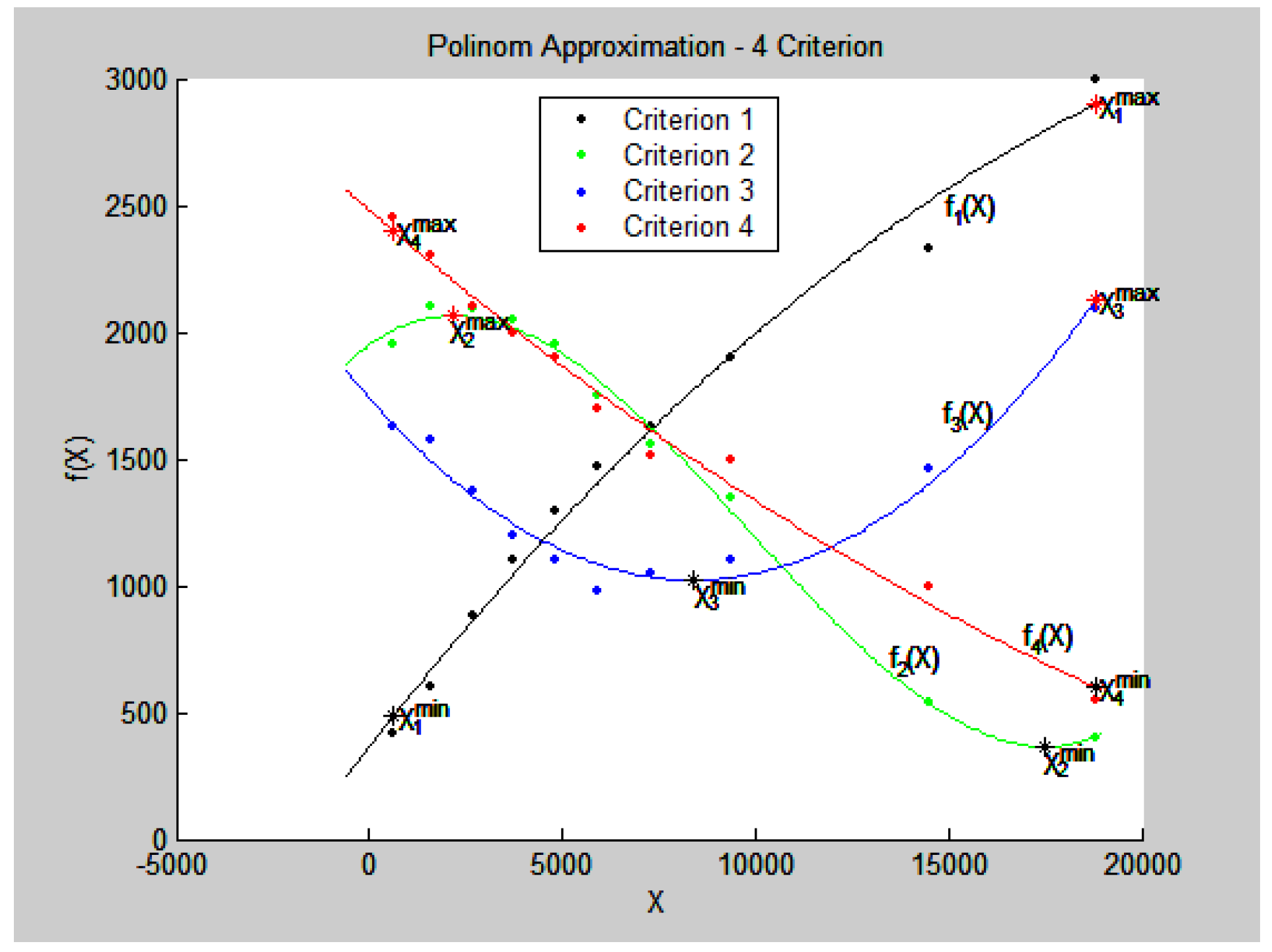
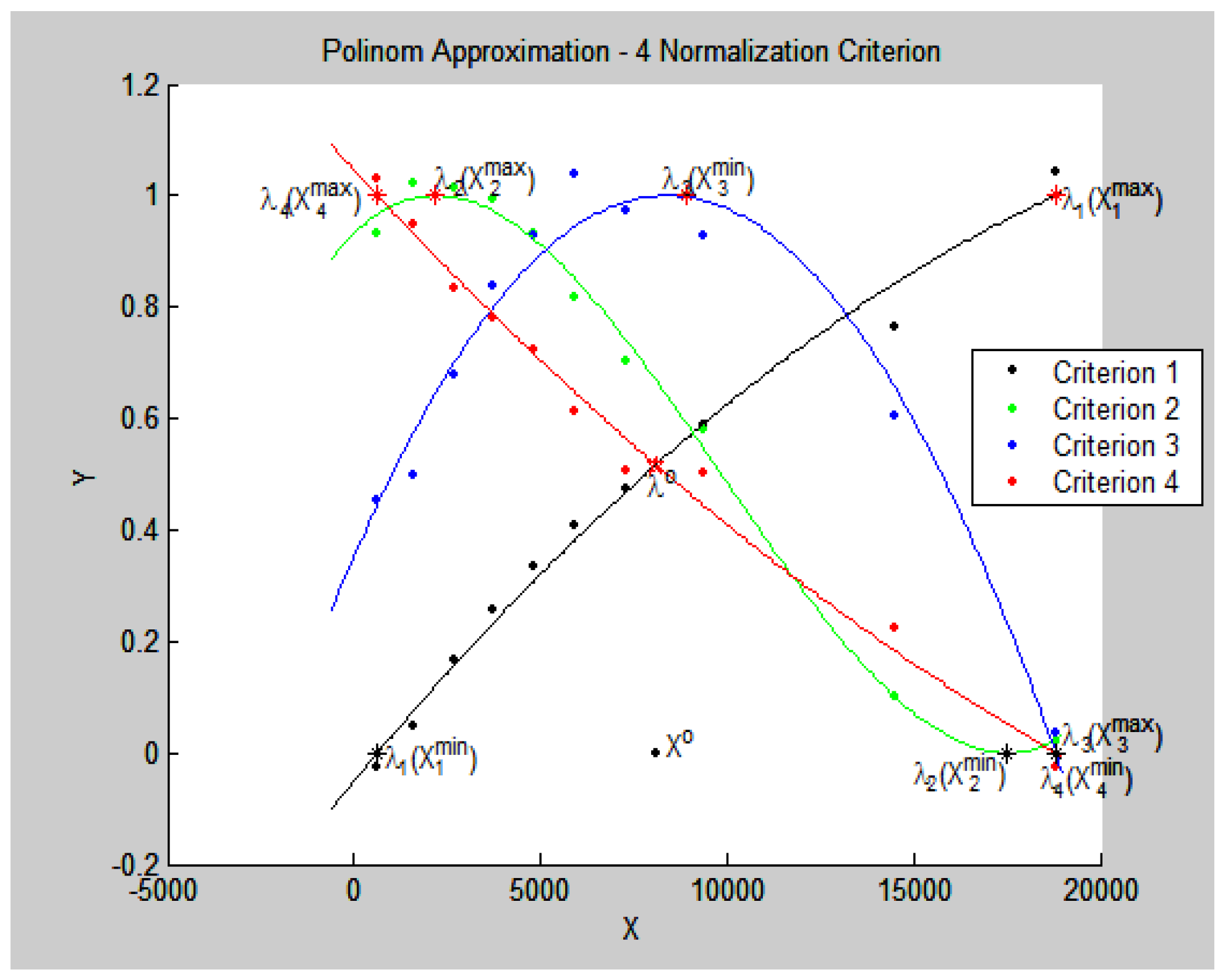
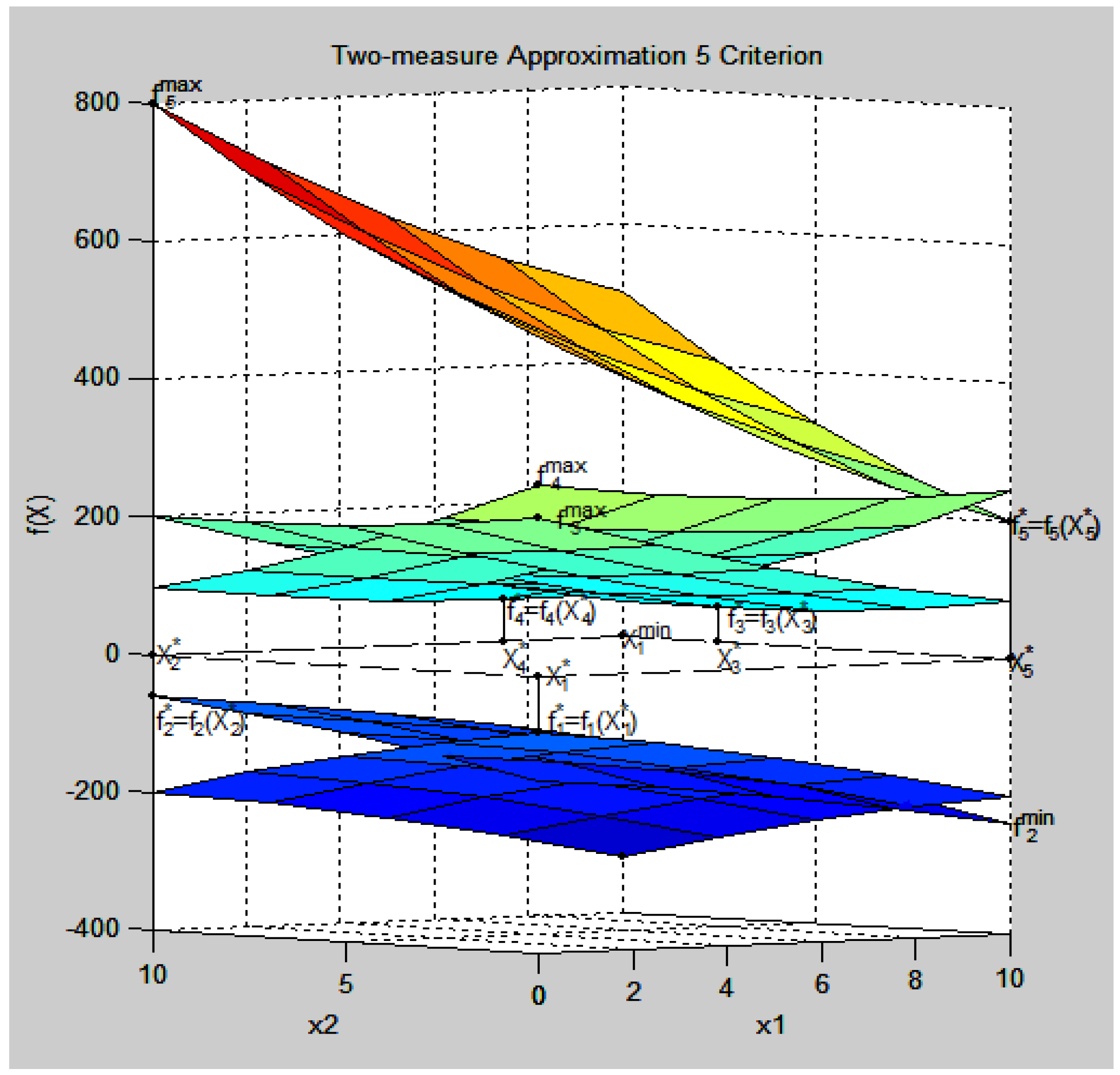
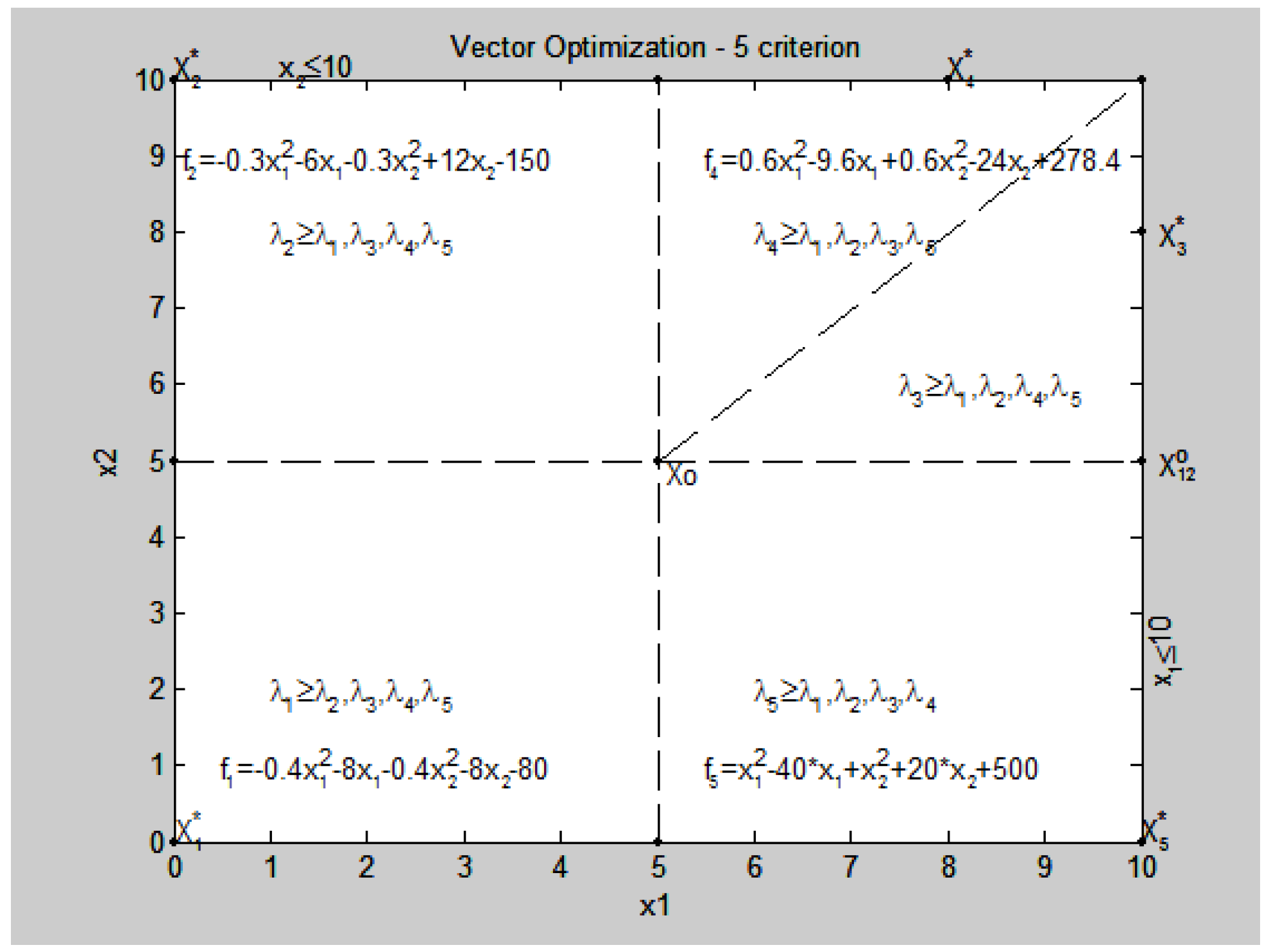
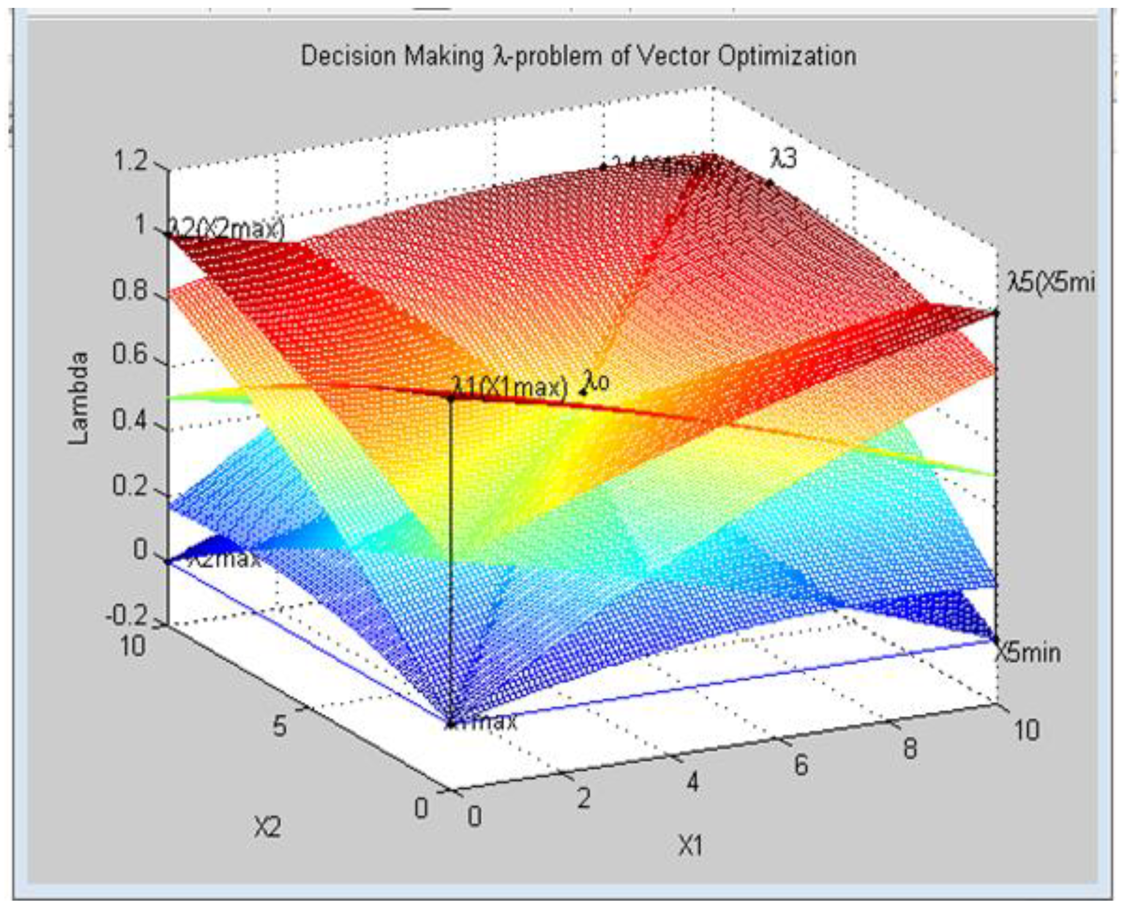
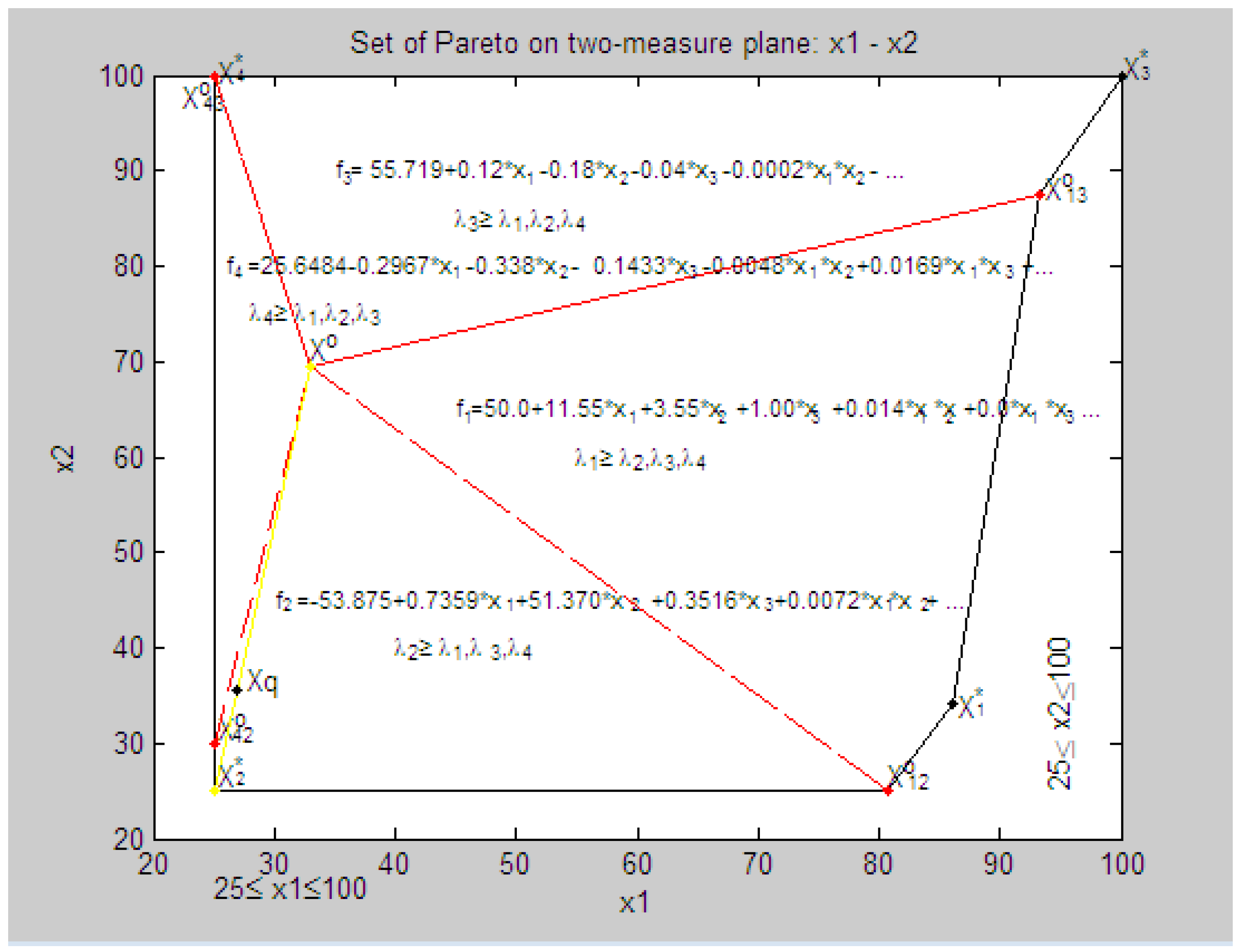
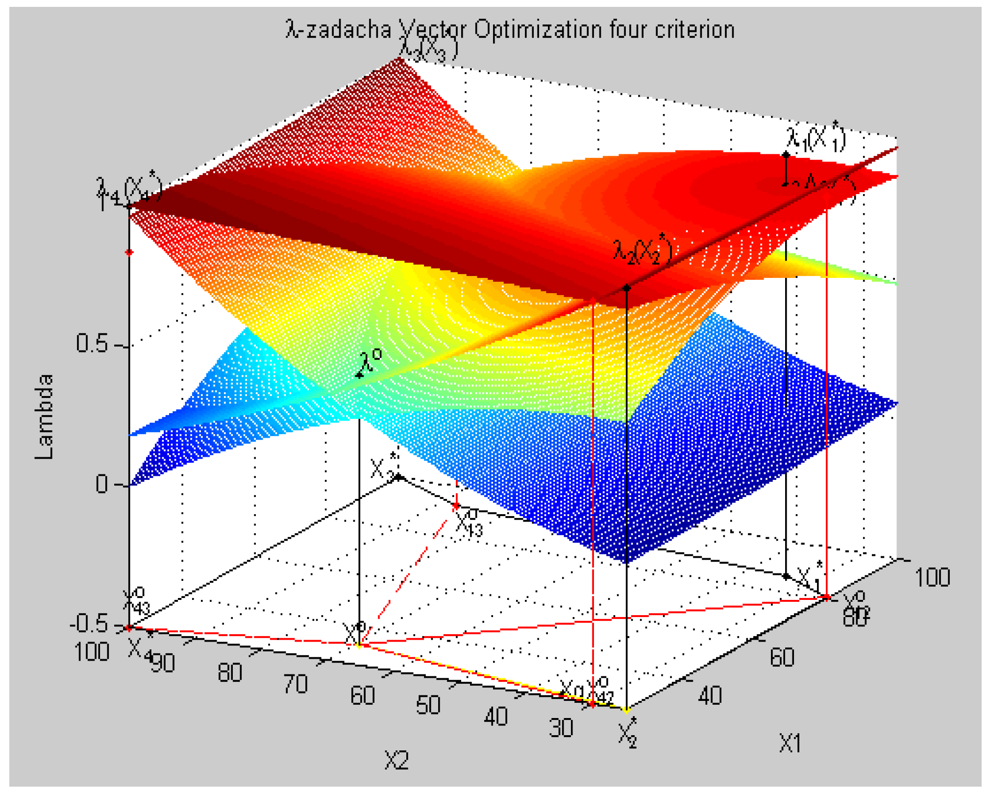
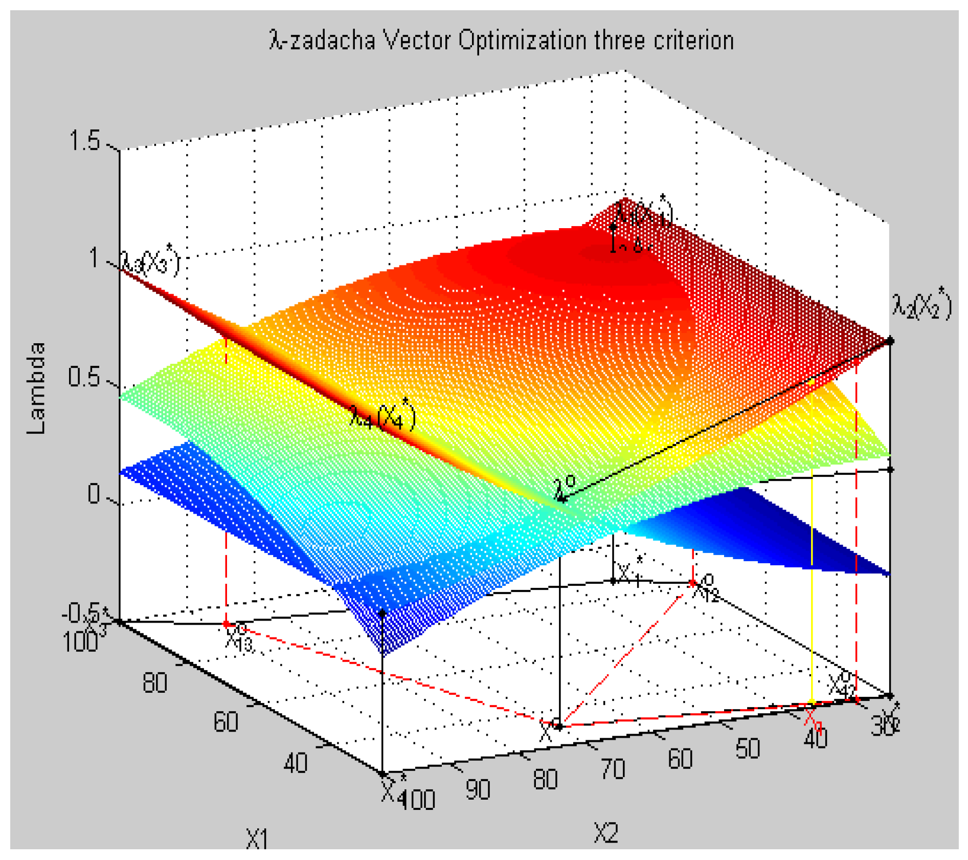
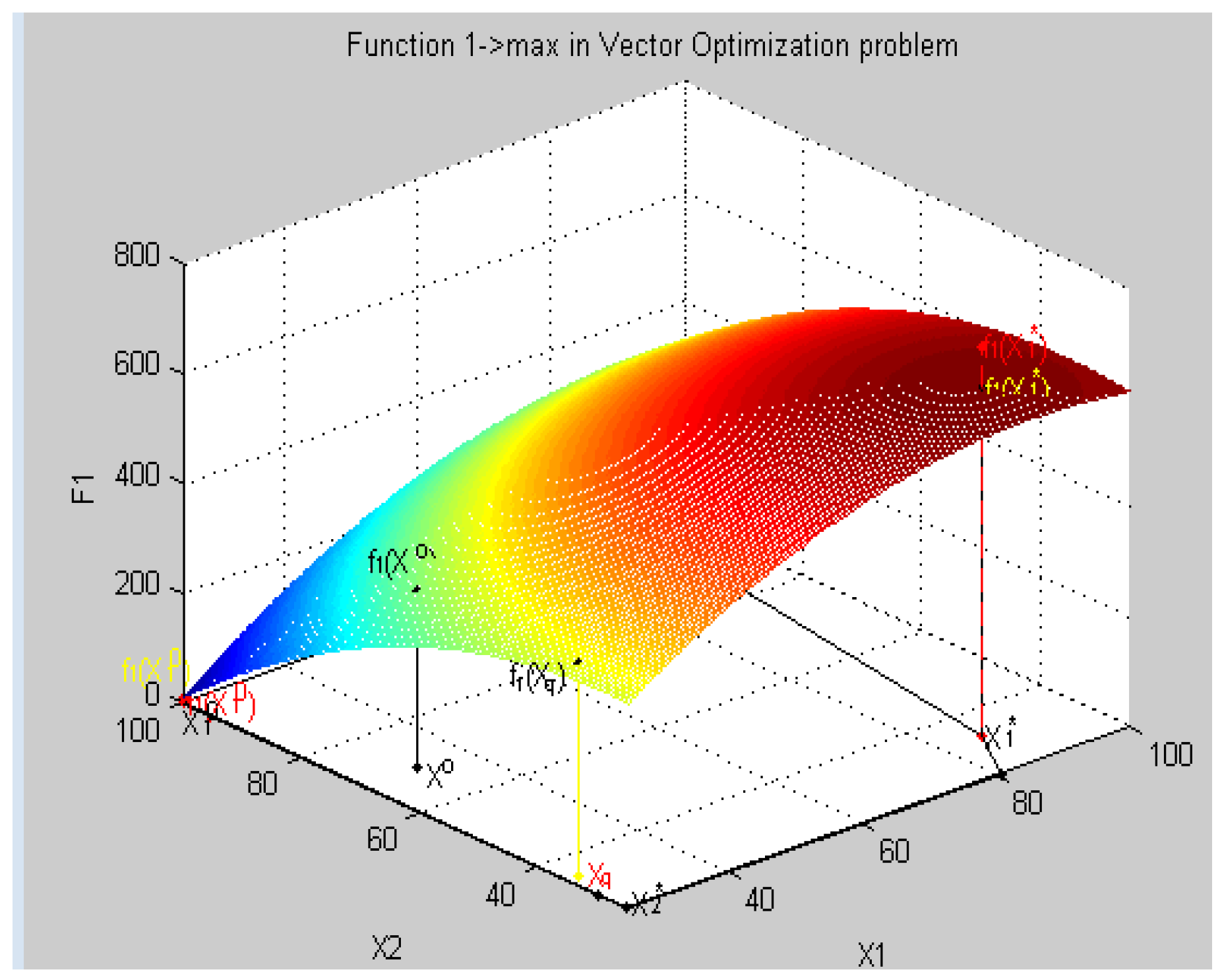
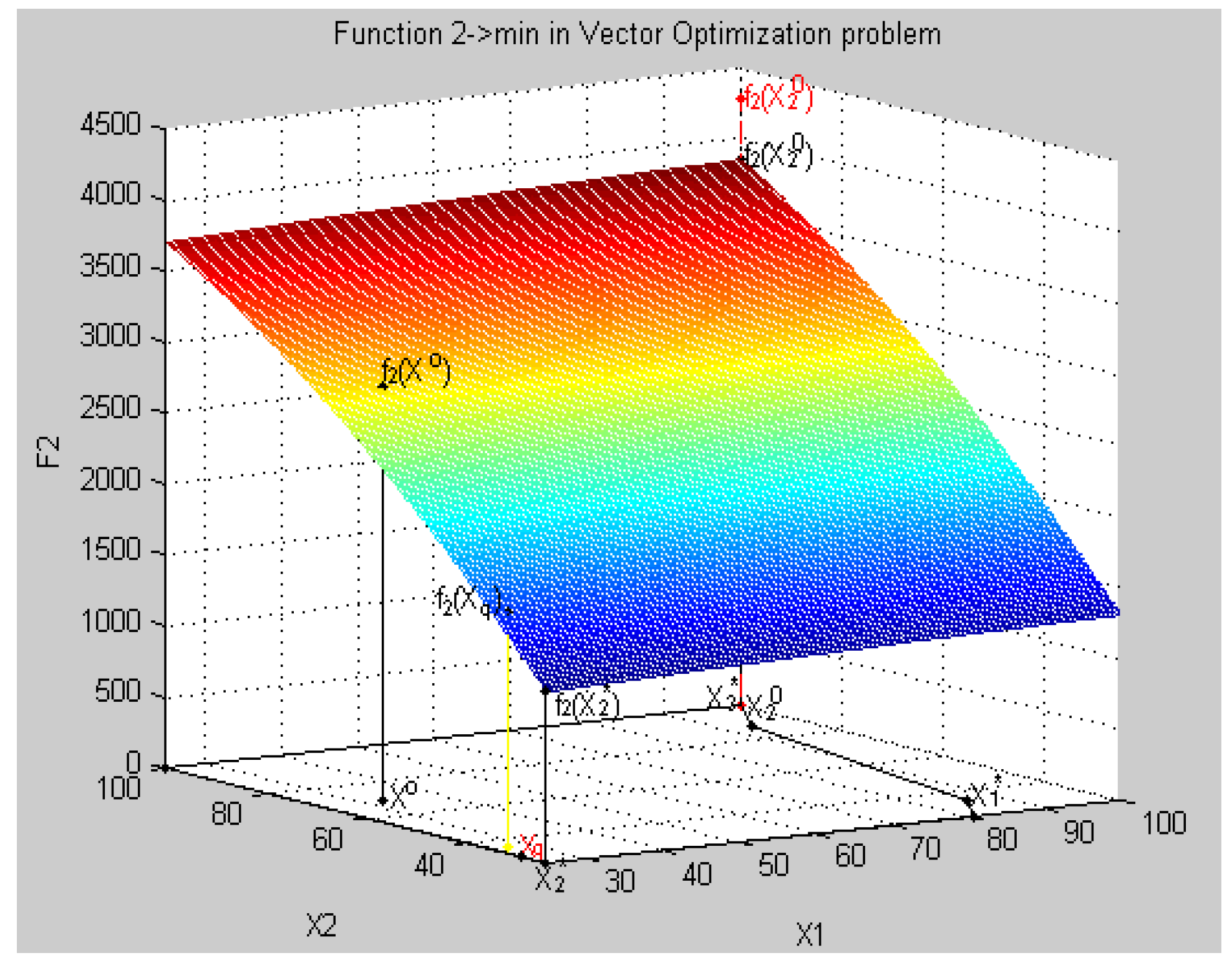
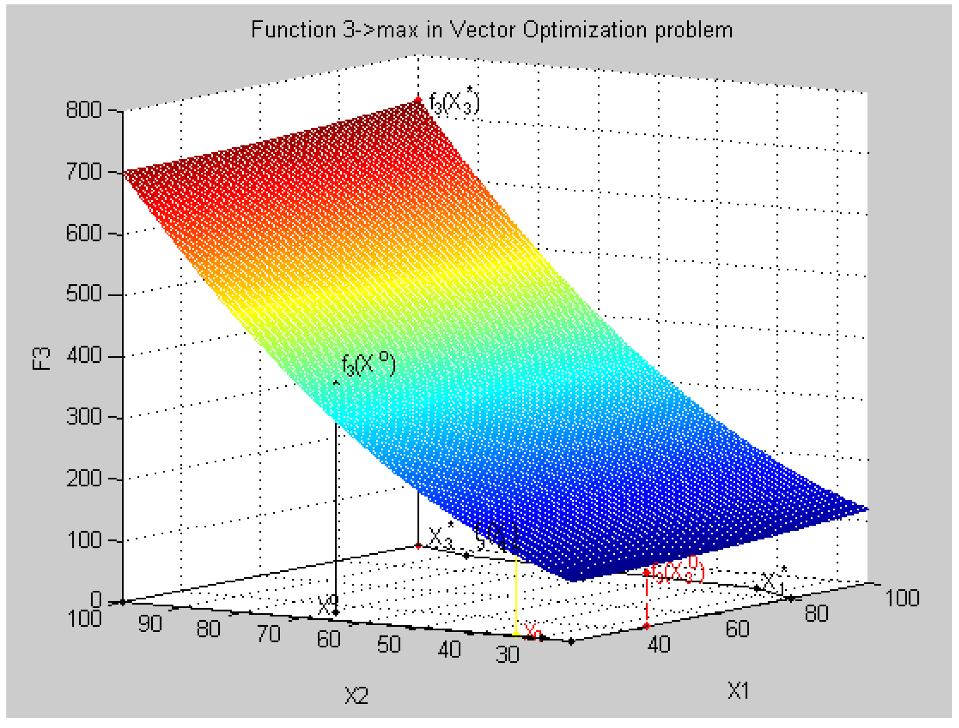
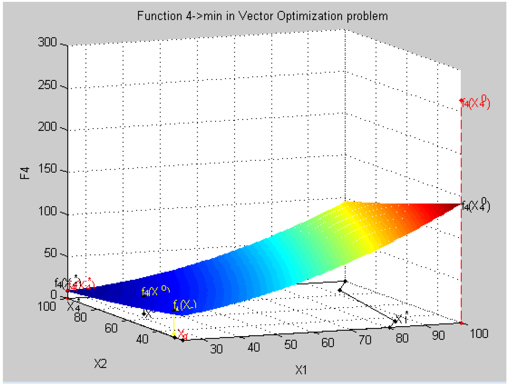
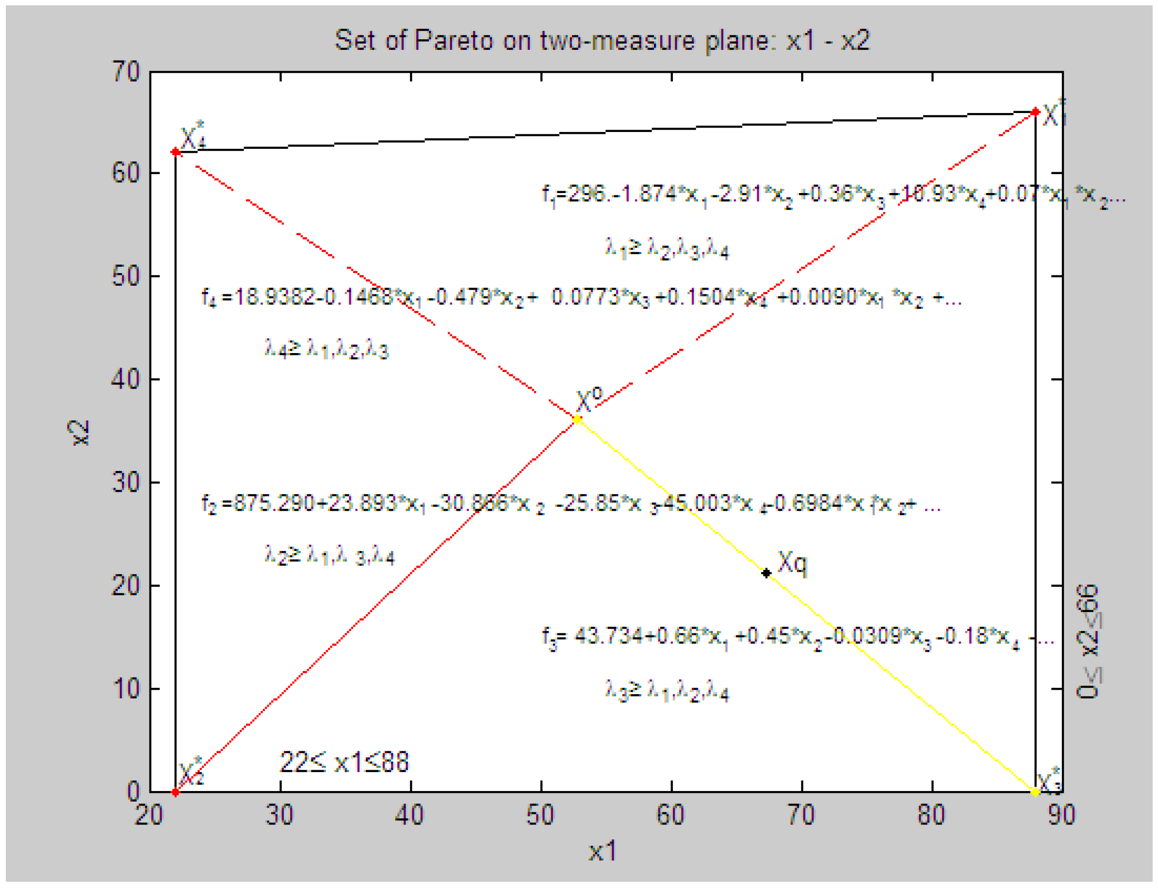
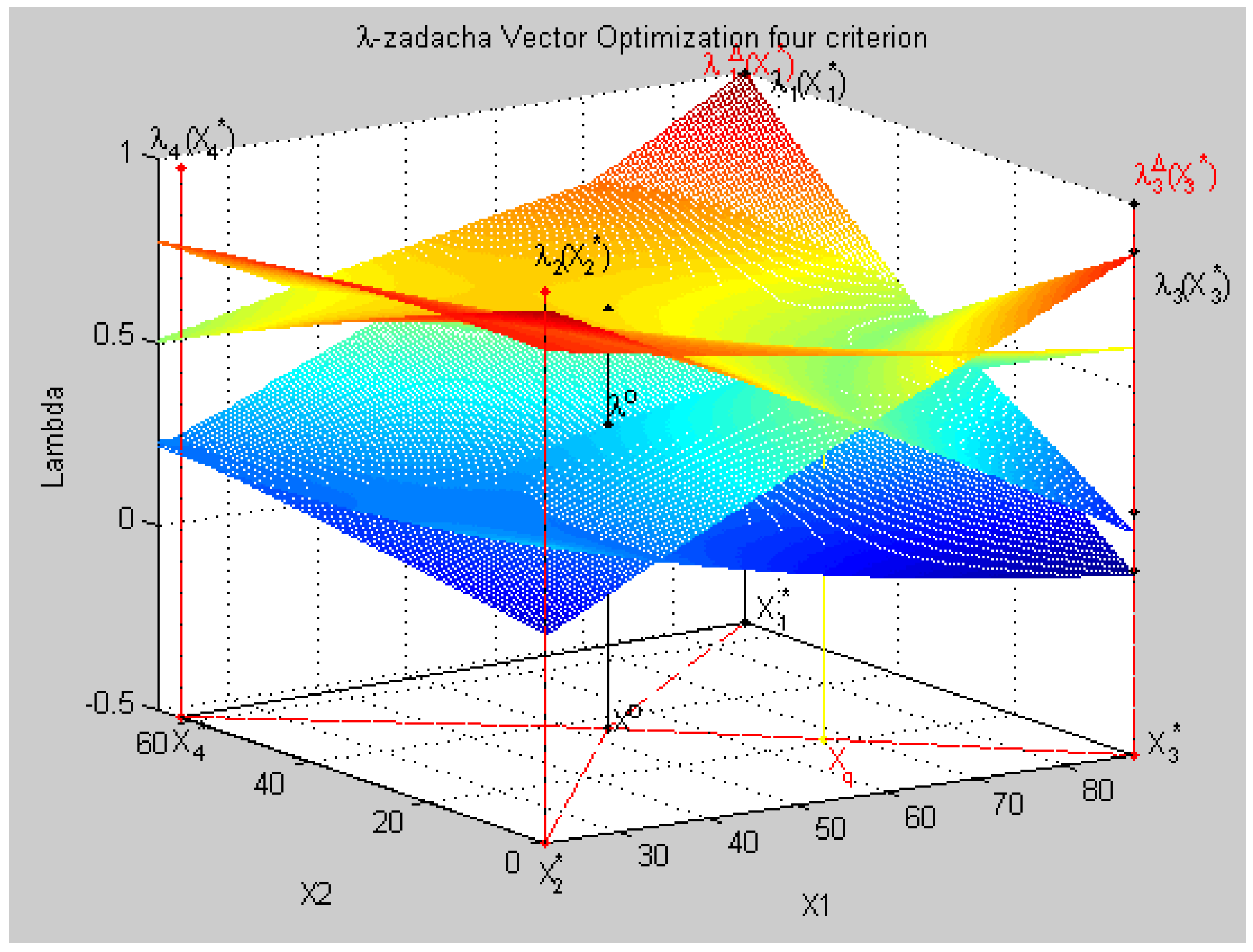
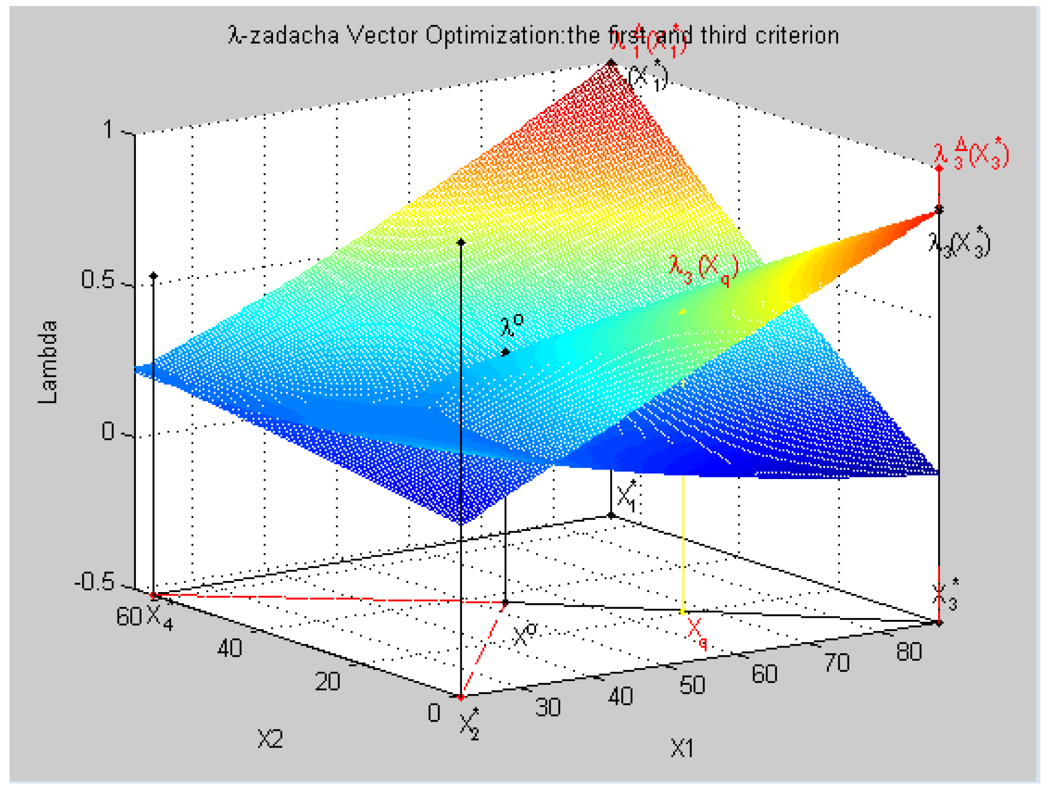
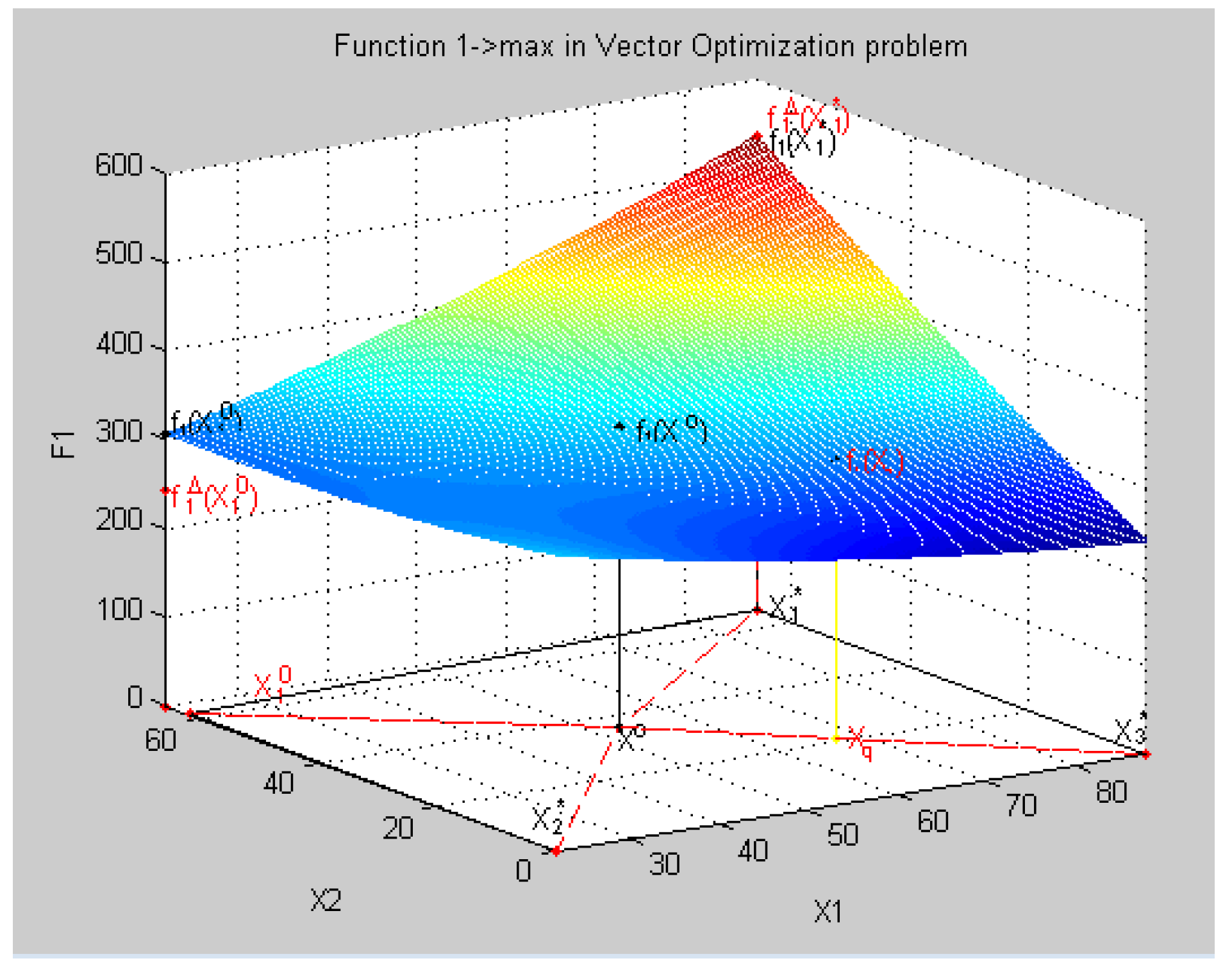
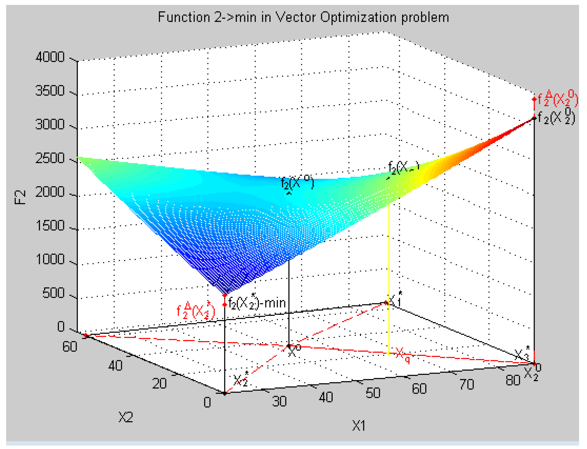
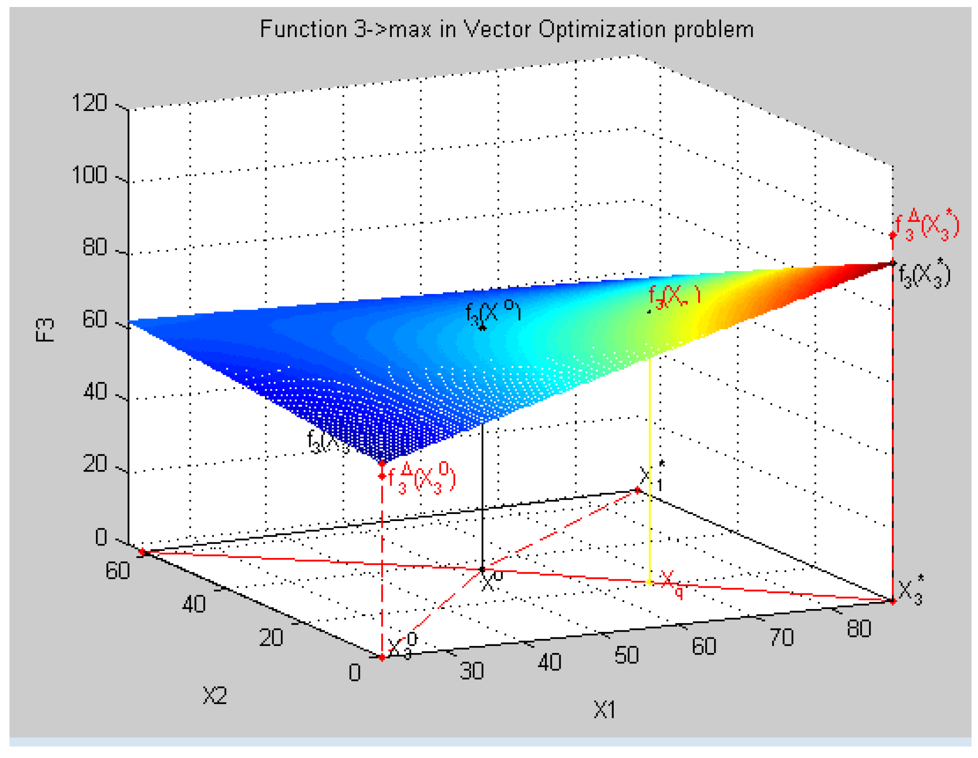
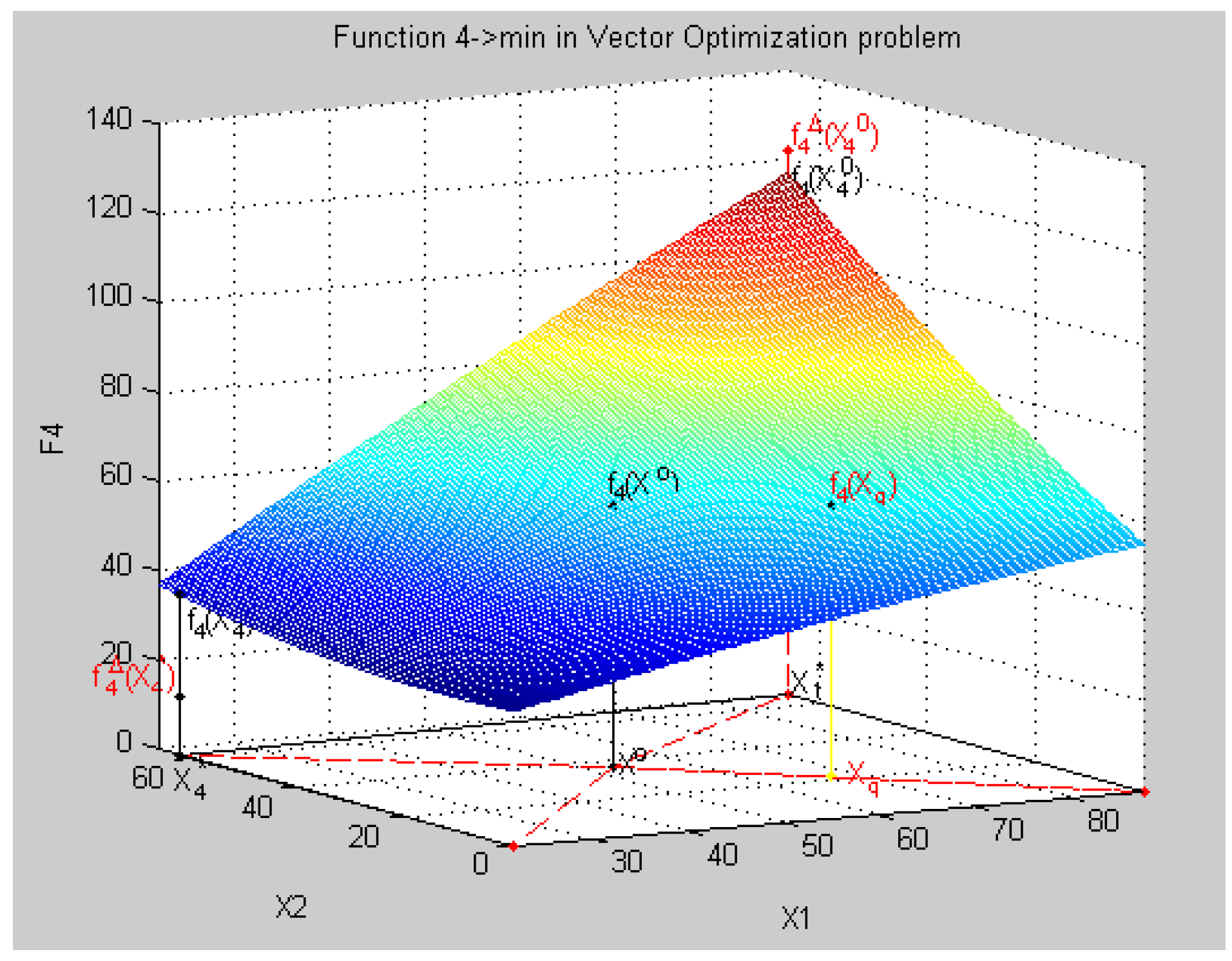
Table 1.
The consumption of resources and operational performance.
| Type Resources | Costs of Resources of One Product | Possibilities of Firm on Resources | |||
|---|---|---|---|---|---|
| Type 1 | Type 2 | Type 3 | Type 4 | ||
| Labor (people/week) | 1 | 1 | 1 | 1 | 15 |
| Material (in kg) | 7 | 5 | 3 | 2 | 120 |
| Capacity (per hour) | 3 | 5 | 10 | 15 | 100 |
| Income from a unit of production | 4.0 | 5.0 | 9.0 | 11.0 | maximize |
| Profit , j = 1,...,4 | 2 | 10 | 6 | 20 | maximize |
| Output | x1 | x2 | x3 | x4 | To define |
Table 2.
Comparing vector problem mathematical programming (VPMP) to decision-making problems (DMP).
Table 2.
Comparing vector problem mathematical programming (VPMP) to decision-making problems (DMP).
| VPMP—Equations (1)–(4) | DMP_1—Equation (37) | DMP_2—Equation (38) |
|---|---|---|
| 2. Common Objective: Making the best decision | ||
| 3. Find the vector X from the admissible set, where the vector criterion F(X) is optimal | Objective: Find the alternative ai, i = , such that the set of criteria , k = is optimal | Objective: Find the vector alternative Xi, i = , such that the set of criteria F(X), is optimal |
| 4. The vector of parameters X and the dependence of criteria F(X) on it are given completely, the set of admissible points is finite: G(X)≤ 0, Xmin ≤ X ≤ Xmax. | Parameters are not given, the criteria are represented as the finite set of values, the set of admissible alternatives is finite | Parameters are given, the criteria are represented as separate values so that the functional dependence between them is not given, the set of admissible points is finite |
| Opt F(X) = {max F1(X) = {max fk(X), k = }, min F2(X) = {min fk(X), k = }}, G(X) ≤ 0, x≤ xj ≤ x, j = | 5. Transforming the Decision Making Problem into VMPP | |
| Using regression analysis, we transform each k-th k = set of values of criteria, , i = into the criterion function fk(x) | Using multiple regression, we transform each k-th k = set of values of criteria , i = into the criterion function | |
| 6. ↑ Problems are Equivalent→ | Opt F(x) = (f1(x))T. ≤ fk(x) ≤ , k = , xmin ≤ x ≤ xmax. | Opt F(X) = (f1(X(X))T. ≤ fk(X) ≤ , k = , Xmin ≤ X ≤ Xmax. |
Table 3.
Experimental data (matrix I).
| x | f1 | f2 | f3 | f4 |
|---|---|---|---|---|
| 630 | 4200 | 1950 | 1628 | 245 |
| 1580 | 6000 | 2100 | 1577 | 230 |
| 2662 | 8850 | 2090 | 1377 | 210 |
| 3704 | 11,000 | 2050 | 1200 | 200 |
| 4800 | 12,900 | 1950 | 1100 | 190 |
| 5929 | 14,730 | 1750 | 977 | 170 |
| 7284 | 16,310 | 1560 | 1050 | 151 |
| 9353 | 19,000 | 1350 | 1100 | 150 |
| 14,505 | 23,250 | 540 | 1457 | 100 |
| 18,810 | 29,970 | 400 | 2088 | 55 |
Table 4.
Normalized criteria.
| x | λ1−max | λ2−max | λ3−min | λ4−max |
|---|---|---|---|---|
| 630 | -0.0276 | 0.933 | 0.451 | 1.0298 |
| 1580 | 0.0471 | 1.0214 | 0.4971 | 0.9463 |
| 2662 | 0.1653 | 1.0155 | 0.6781 | 0.8351 |
| 3704 | 0.2545 | 0.9919 | 0.8383 | 0.7795 |
| 4800 | 0.3334 | 0.933 | 0.9289 | 0.7239 |
| 5929 | 0.4093 | 0.8153 | 1.0402 | 0.6127 |
| 7284 | 0.4748 | 0.7034 | 0.9741 | 0.507 |
| 9353 | 0.5864 | 0.5798 | 0.9289 | 0.5014 |
| 14,505 | 0.7627 | 0.1029 | 0.6057 | 0.2234 |
| 18,810 | 1.0415 | 0.0205 | 0.0346 | −0.0269 |
Table 5.
Experimental data (matrix I).
| x1 | x2 | f1 | f2 | f3 | f4 | f5 |
|---|---|---|---|---|---|---|
| 0 | 0 | −80 | −150 | 232 | 278.4 | 500 |
| 0 | 2.5 | −102.5 | −121.875 | 215.125 | 222.15 | 556.25 |
| 0 | 5 | −130 | −97.5 | 204.5 | 173.4 | 625 |
| 0 | 7.5 | −162.5 | −76.875 | 200.125 | 132.15 | 706.25 |
| 0 | 10 | −200 | −60 | 202 | 98.4 | 800 |
| 2.5 | 0 | −102.5 | −166.875 | 185.125 | 258.15 | 406.25 |
| 2.5 | 2.5 | −125 | −138.75 | 168.25 | 201.9 | 462.5 |
| 2.5 | 5 | −152.5 | −114.375 | 157.625 | 153.15 | 531.25 |
| 2.5 | 7.5 | −185 | −93.75 | 153.25 | 111.9 | 612.5 |
| 2.5 | 10 | −222.5 | −76.875 | 155.125 | 78.15 | 706.25 |
| 5 | 0 | −130 | −187.5 | 144.5 | 245.4 | 325 |
| 5 | 2.5 | −152.5 | −159.375 | 127.625 | 189.15 | 381.25 |
| 5 | 5 | −180 | −135 | 117 | 140.4 | 450 |
| 5 | 7.5 | −212.5 | −114.375 | 112.625 | 99.15 | 531.25 |
| 5 | 10 | −250 | −97.5 | 114.5 | 65.4 | 625 |
| 7.5 | 0 | −162.5 | −211.875 | 110.125 | 240.15 | 256.25 |
| 7.5 | 2.5 | −185 | −183.75 | 93.25 | 183.9 | 312 |
| 7.5 | 5 | −212.5 | −159.375 | 82.625 | 135.15 | 381.25 |
| 7.5 | 7.5 | −245 | −138.75 | 78.25 | 93.9 | 462.5 |
| 7.5 | 10 | −282.5 | −121.875 | 80.125 | 60.15 | 556.25 |
| 10 | 0 | −200 | −240 | 82 | 242.4 | 200 |
| 10 | 2.5 | −222.5 | −211.875 | 65.125 | 186.15 | 256.25 |
| 10 | 5 | −250 | −187.5 | 54.5 | 137.4 | 325 |
| 10 | 7.5 | −282.5 | −166.875 | 50.125 | 96.15 | 406.25 |
| 10 | 10 | −320 | −150 | 52 | 62.4 | 500 |
Table 6.
Numerical values of parameters and characteristics of the system.
| x1 | x2 | x3 | y1(X) → max | y2(X) → min |
|---|---|---|---|---|
| 25 | 25 | 25 | 412.5 | 1197.2 |
| 25 | 25 | 50 | 437.5 | 1232.8 |
| 25 | 25 | 75 | 462.5 | 1393.3 |
| 25 | 25 | 100 | 87.5 | 1303.8 |
| 25 | 50 | 25 | 312.5 | 2232.3 |
| 25 | 50 | 50 | 37.5 | 2267.7 |
| 25 | 50 | 75 | 62.5 | 2303.2 |
| 25 | 50 | 100 | 87.5 | 2338.8 |
| 25 | 75 | 25 | 212.5 | 3077.2 |
| 25 | 75 | 50 | 237.5 | 2862.8 |
| 25 | 75 | 75 | 262.5 | 3148.3 |
| 25 | 75 | 100 | 287.5 | 3183.7 |
| 25 | 100 | 25 | 12.5 | 3732.3 |
| 25 | 100 | 50 | 37.5 | 3767.7 |
| 25 | 100 | 75 | 62.5 | 3803.2 |
| 25 | 100 | 100 | 87.5 | 3838.8 |
| 50 | 25 | 25 | 512.5 | 1245.3 |
| 50 | 25 | 50 | 537.5 | 1303.8 |
| 50 | 25 | 75 | 562.5 | 1374.7 |
| 50 | 25 | 100 | 587.5 | 1445.8 |
| 50 | 50 | 25 | 512.5 | 2267.7 |
| 50 | 50 | 50 | 537.5 | 2338.8 |
| 50 | 50 | 75 | 562.5 | 2409.7 |
| 50 | 50 | 100 | 587.5 | 2480.8 |
| 50 | 75 | 25 | 412.5 | 3112.8 |
| 50 | 75 | 50 | 437.5 | 3183.7 |
| 50 | 75 | 75 | 462.5 | 3379.8 |
| 50 | 75 | 100 | 487.5 | 3325.8 |
| 50 | 100 | 25 | 212.5 | 3767.7 |
| 50 | 100 | 50 | 237.5 | 3838.8 |
| 50 | 100 | 75 | 262.5 | 3909.7 |
| 50 | 100 | 100 | 287.5 | 3980.8 |
| 75 | 25 | 25 | 612.5 | 1268.3 |
| 75 | 25 | 50 | 637.5 | 1374.7 |
| 75 | 25 | 75 | 662.5 | 1481.3 |
| 75 | 25 | 100 | 687.5 | 1587.8 |
| 75 | 50 | 25 | 612.5 | 2303.2 |
| 75 | 50 | 50 | 637.5 | 2409.7 |
| 75 | 50 | 75 | 662.5 | 2516.2 |
| 75 | 50 | 100 | 687.5 | 2622.7 |
| 75 | 75 | 25 | 512.5 | 3148.3 |
| 75 | 75 | 50 | 537.5 | 3254.8 |
| 75 | 75 | 75 | 562.5 | 3361.3 |
| 75 | 75 | 100 | 587.5 | 3467.8 |
| 75 | 100 | 25 | 312.5 | 3803.2 |
| 75 | 100 | 50 | 337.5 | 3909.7 |
| 75 | 100 | 75 | 362.5 | 4016.3 |
| 75 | 100 | 100 | 387.5 | 4122.7 |
| 100 | 25 | 25 | 612.5 | 1303.8 |
| 100 | 25 | 50 | 637.5 | 1445.8 |
| 100 | 25 | 75 | 662.5 | 1587.8 |
| 100 | 25 | 100 | 687.5 | 1729.7 |
| 100 | 50 | 25 | 612.5 | 2338.8 |
| 100 | 50 | 50 | 637.5 | 2480.8 |
| 100 | 50 | 75 | 662.5 | 2622.7 |
| 100 | 50 | 100 | 687.5 | 2764.7 |
| 100 | 75 | 25 | 512.5 | 3183.7 |
| 100 | 75 | 50 | 537.5 | 3325.8 |
| 100 | 75 | 75 | 562.5 | 3467.8 |
| 100 | 75 | 100 | 587.5 | 3609.8 |
| 100 | 100 | 25 | 312.5 | 3838.8 |
| 100 | 100 | 50 | 337.5 | 3980.8 |
| 100 | 100 | 75 | 362.5 | 4122.7 |
| 100 | 100 | 100 | 387.5 | 4264.8 |
Table 7.
Numerical values of parameters and characteristics of the system.
| x1 | x2 | x3 | x4 | y2(X) →min | y3(X) →max |
|---|---|---|---|---|---|
| 22 | 0 | 2.2 | 2.2 | 1053.8 | 47.7 |
| 22 | 0 | 2.2 | 5.5 | 1067 | 47.3 |
| 22 | 0 | 2.2 | 8.8 | 1078 | 47.2 |
| 22 | 0 | 5.5 | 2.2 | 1111 | 50.7 |
| 22 | 0 | 5.5 | 5.5 | 1155 | 46.8 |
| 22 | 0 | 5.5 | 8.8 | 1152.8 | 46.3 |
| 22 | 0 | 8.8 | 2.2 | 1151.7 | 44.2 |
| 22 | 0 | 8.8 | 5.5 | 1148.4 | 43 |
| 22 | 0 | 8.8 | 8.8 | 1147.3 | 42.5 |
| 22 | 33 | 2.2 | 2.2 | 1964.6 | 58.3 |
| 22 | 33 | 2.2 | 5.5 | 1974.5 | 57.5 |
| 22 | 33 | 2.2 | 8.8 | 1983.3 | 57.1 |
| 22 | 33 | 5.5 | 2.2 | 1995.4 | 56.5 |
| 22 | 33 | 5.5 | 5.5 | 2003.1 | 55.1 |
| 22 | 33 | 5.5 | 8.8 | 2015.2 | 54.9 |
| 22 | 33 | 8.8 | 2.2 | 2027.3 | 54.8 |
| 22 | 33 | 8.8 | 5.5 | 2046 | 52.8 |
| 22 | 33 | 8.8 | 8.8 | 2058.1 | 53 |
| 22 | 66 | 2.2 | 2.2 | 2708.2 | 75.9 |
| 22 | 66 | 2.2 | 5.5 | 2585 | 71.5 |
| 22 | 66 | 2.2 | 8.8 | 2541 | 68.2 |
| 22 | 66 | 5.5 | 2.2 | 2519 | 66.4 |
| 22 | 66 | 5.5 | 5.5 | 2596 | 68.2 |
| 22 | 66 | 5.5 | 8.8 | 2662 | 70.4 |
| 22 | 66 | 8.8 | 2.2 | 2770.9 | 72.4 |
| 22 | 66 | 8.8 | 5.5 | 2783 | 71.5 |
| 22 | 66 | 8.8 | 8.8 | 2801.7 | 70.6 |
| 55 | 0 | 2.2 | 2.2 | 3284.6 | 100.5 |
| 55 | 0 | 2.2 | 5.5 | 3301.1 | 100.1 |
| 55 | 0 | 2.2 | 8.8 | 3307.7 | 99 |
| 55 | 0 | 5.5 | 2.2 | 3315.4 | 98.8 |
| 55 | 0 | 5.5 | 5.5 | 3320.9 | 97.9 |
| 55 | 0 | 5.5 | 8.8 | 3334.1 | 97.6 |
| 55 | 0 | 8.8 | 2.2 | 3347.3 | 97 |
| 55 | 0 | 8.8 | 5.5 | 3366 | 95.7 |
| 55 | 0 | 8.8 | 8.8 | 3378.1 | 95.3 |
| 55 | 33 | 2.2 | 2.2 | 1095.6 | 54.6 |
| 55 | 33 | 2.2 | 5.5 | 1111 | 50.6 |
| 55 | 33 | 2.2 | 8.8 | 1133 | 48.4 |
| 55 | 33 | 5.5 | 2.2 | 1147.3 | 47.7 |
| 55 | 33 | 5.5 | 5.5 | 1166 | 46.2 |
| 55 | 33 | 5.5 | 8.8 | 1188 | 45.1 |
| 55 | 33 | 8.8 | 2.2 | 1208.9 | 44.2 |
| 55 | 33 | 8.8 | 5.5 | 1232 | 42.2 |
| 55 | 33 | 8.8 | 8.8 | 1272.7 | 40.7 |
| 55 | 66 | 2.2 | 2.2 | 1995.4 | 61.8 |
| 55 | 66 | 2.2 | 5.5 | 2013 | 60.5 |
| 55 | 66 | 2.2 | 8.8 | 2035 | 59.4 |
| 55 | 66 | 5.5 | 2.2 | 2058.1 | 58.3 |
| 55 | 66 | 5.5 | 5.5 | 2095.5 | 57.2 |
| 55 | 66 | 5.5 | 8.8 | 2103.2 | 56.1 |
| 55 | 66 | 8.8 | 2.2 | 2120.8 | 54.8 |
| 55 | 66 | 8.8 | 5.5 | 2145 | 47.3 |
| 55 | 66 | 8.8 | 8.8 | 2183.5 | 51.3 |
| 88 | 0 | 2.2 | 2.2 | 2739 | 79.4 |
| 88 | 0 | 2.2 | 5.5 | 2761 | 78.1 |
| 88 | 0 | 2.2 | 8.8 | 2783 | 77 |
| 88 | 0 | 5.5 | 2.2 | 2801.7 | 75.9 |
| 88 | 0 | 5.5 | 5.5 | 2849 | 76.1 |
| 88 | 0 | 5.5 | 8.8 | 2893 | 76.6 |
| 88 | 0 | 8.8 | 2.2 | 2974.4 | 76.8 |
| 88 | 0 | 8.8 | 5.5 | 2959 | 715 |
| 88 | 0 | 8.8 | 8.8 | 2927.1 | 682 |
| 88 | 33 | 2.2 | 2.2 | 3315.4 | 1041 |
| 88 | 33 | 2.2 | 5.5 | 3336.3 | 1023 |
| 88 | 33 | 2.2 | 8.8 | 3355 | 1012 |
| 88 | 33 | 5.5 | 2.2 | 3378.1 | 1005 |
| 88 | 33 | 5.5 | 5.5 | 3399 | 990 |
| 88 | 33 | 5.5 | 8.8 | 3421 | 979 |
| 88 | 33 | 8.8 | 2.2 | 3440.8 | 970 |
| 88 | 33 | 8.8 | 5.5 | 3366 | 957 |
| 88 | 33 | 8.8 | 8.8 | 3503.5 | 935 |
| 88 | 66 | 2.2 | 2.2 | 1116.5 | 583 |
| 88 | 66 | 2.2 | 5.5 | 1144 | 561 |
| 88 | 66 | 2.2 | 8.8 | 1166 | 550 |
| 88 | 66 | 5.5 | 2.2 | 1208.9 | 530 |
| 88 | 66 | 5.5 | 5.5 | 1232 | 506 |
| 88 | 66 | 5.5 | 8.8 | 1276 | 484 |
| 88 | 66 | 8.8 | 2.2 | 1303.5 | 477 |
| 88 | 66 | 8.8 | 5.5 | 1342 | 440 |
| 88 | 66 | 8.8 | 8.8 | 1397 | 425 |
© 2019 by the author. Licensee MDPI, Basel, Switzerland. This article is an open access article distributed under the terms and conditions of the Creative Commons Attribution (CC BY) license (http://creativecommons.org/licenses/by/4.0/).
Share and Cite
MDPI and ACS Style
Mashunin, Y.K. Mathematical Apparatus of Optimal Decision-Making Based on Vector Optimization. Appl. Syst. Innov. 2019, 2, 32. https://0-doi-org.brum.beds.ac.uk/10.3390/asi2040032
AMA Style
Mashunin YK. Mathematical Apparatus of Optimal Decision-Making Based on Vector Optimization. Applied System Innovation. 2019; 2(4):32. https://0-doi-org.brum.beds.ac.uk/10.3390/asi2040032
Chicago/Turabian StyleMashunin, Yury K. 2019. "Mathematical Apparatus of Optimal Decision-Making Based on Vector Optimization" Applied System Innovation 2, no. 4: 32. https://0-doi-org.brum.beds.ac.uk/10.3390/asi2040032