Performance Assessment of a Low-Cost PM2.5 Sensor for a near Four-Month Period in Oslo, Norway

NILU—Norwegian Institute for Air Research, Postboks 100, 2027 Kjeller, Norway
*
Author to whom correspondence should be addressed.
Atmosphere 2019, 10(2), 41; https://0-doi-org.brum.beds.ac.uk/10.3390/atmos10020041
Submission received: 18 December 2018
/
Revised: 16 January 2019
/
Accepted: 21 January 2019
/
Published: 22 January 2019
(This article belongs to the Special Issue Sensors for Air Quality Assessment)
Abstract
:The very low-cost Nova particulate matter (PM) sensor SDS011 has recently drawn attention for its use for measuring PM mass concentration, which is frequently used as an indicator of air quality. However, this sensor has not been thoroughly evaluated in real-world conditions and its data quality is not well documented. In this study, three SDS011 sensors were evaluated by co-locating them at an official, air quality monitoring station equipped with reference-equivalent instrumentation in Oslo, Norway. The sensors’ measurement results for PM2.5 were compared with data generated from the air quality monitoring station over almost a four-month period. Five performance aspects of the sensors were examined: operational data coverage, linearity of response and accuracy, inter-sensor variability, dependence on relative humidity (RH) and temperature (T), and potential improvement of sensor accuracy, by data calibration using a machine-learning method. The results of the study are: (i) the three sensors provide quite similar results, with inter-sensor correlations exhibiting R values higher than 0.97; (ii) all three sensors demonstrate quite high linearity against officially measured concentrations of PM2.5, with R2 values ranging from 0.55 to 0.71; (iii) high RH (over 80%) negatively affected the sensor response; (iv) data calibration using only the RH and T recorded directly at the three sensors increased the R2 value from 0.71 to 0.80, 068 to 0.79, and 0.55 to 0.76. The results demonstrate the general feasibility of using these low cost SDS011 sensors for indicative PM2.5 monitoring under certain environmental conditions. Within these constraints, they further indicate that there is potential for deploying large networks of such devices, due to the sensors’ relative accuracy, size and cost. This opens up a wide variety of applications, such as high-resolution air quality mapping and personalized air quality information services. However, it should be noted that the sensors exhibit often very high relative errors for hourly values and that there is a high potential of abusing these types of sensors if they are applied outside the manufacturer-provided specifications particularly regarding relative humidity. Furthermore, our analysis covers only a relatively short time period and it is desirable to carry out longer-term studies covering a wider range of meteorological conditions.
1. Introduction
Particulate matter (PM) is one of the major airborne pollutants in urban environments and is one of the most problematic air pollutants, in terms of its negative effects on human health [1]. The effects of PM on human health, which have been widely studied in the last twenty years, include asthma, lung cancer and cardiovascular issues [2,3]. Generally, the level of health effects from PM are related to the size of particles. For instance, PM up to 10 micro-meters (μm) in diameter (PM10,) can penetrate into the bronchi. PM up to 2.5 μm (PM2.5, fine particles) can penetrate the lungs, while ultrafine particles (PM0.1) are able to pass through the lung tissue and enter the circulatory system [4,5]. The International Agency for Research on Cancer (IARC) concluded in 2013 that PM is carcinogenic to humans [6]. According to the European Environmental Agency (EEA), in 2014, 428,000 premature deaths in 41 European countries were caused by PM2.5 in the air [7].
Traditionally, like most other pollutants, PM concentration is measured at fixed air quality monitoring stations by using accurate and expensive instrumentation. In the European Union, the density of such networks of monitoring stations is determined by the EU Air Quality Directive 2008/50/EC, which defines the minimum number of fixed monitoring stations for each target pollutant based on the air pollution levels, population and coverage area [8]. However, due to the substantial cost associated with setting up and maintaining such stations, the number of monitoring sites tends to be quite small in most areas, and, while the resulting networks are capable of fulfilling the regulatory needs, their number is generally insufficient for providing detailed information about the spatial distribution of the pollutants, identify pollution hotspots, or provide comprehensive personalized information about air quality to citizens at locations not covered by the network. Although pollutant dispersion models can be used to address this issue to some extent, they often exhibit bias [9,10]. Integrating the observations from a dense network of low-cost sensors with model information through techniques such as data fusion and data assimilation is able to provide spatially continuous concentration fields with significantly reduced bias [11,12,13]. This adds values to the sensor observations by spatially interpolating between monitoring locations and at the same adds value to the model by constraining the model with actual observations. As such, the advantages of both datasets are combined in a mathematically objective fashion, and the resulting up-to-date concentration fields allow for the possibility of providing more relevant personalized information about air quality and exposure to the public.
The recent advancements in the field of low-cost micro-sensors and information and communication technology (ICT) are an opportunity to realise this objective of providing up-to-date and useful air quality information by complementing the official outdoor air quality monitoring networks and improving the spatial and temporal resolution of air quality data [13,14,15,16].
Currently, several categories of low-cost micro-sensors for PM measurements are available, e.g. Sharp GP2Y1010 [17], Shinyei PPD42NS [18], Plantower PMS1003 [19,20], Nova SDS011 [21], AirBeam [22], Alphasense Optical Particle Counter (OPC-N2) [23], and Wuhan Cubic PM3007 [24]. These sensors are all based on optical light scattering using a laser and applying Mie theory on the scattered light to determine the particle size [25]. These PM sensors come in compact sizes, are light, have low energy consumption, operate at a high sampling frequency, and cost from tens to hundreds of Euros each [26]. Such sensors are promising to be deployed in the outdoor environment in terms of their size, cost and ease of use. In particular, such sensors have already been used among non-profit organisations and citizen scientists [27]. However, it is crucial that the sensors’ accuracy, precision and reliability are assessed in a comprehensive and repeatable manner under real-world conditions before they are deployed in large numbers [27].
So far, only a limited number of studies have evaluated this new generation of low-cost sensors for PM2.5 monitoring, and their performance under various environmental conditions and different time scales is still not well understood [28]. Genikomsakis et al. (2018) [29] performed an on-field testing of low-cost portable system for monitoring PM2.5 concentrations in Thessaloniki (Greece), by using a Nova PM sensor SDS011 with an equipped calibrated instrument as the basis of comparison, during the period of 6–8 March 2017. Their results showed that the Nova PM sensor SDS011 maintained a high level of accuracy (R2 value ranging from 0.93 to 0.95) despite of the errors introduced due to the conditions of the mobile test run. Badura et al. (2018) [30] conducted a performance assessment for Nova PM sensor SDS011, ZH03A (Winsen), PMS7003 (Plantower), and OPC-N2 (Alphasense) sensors, with a TEOM 1400a analyser for almost half a year from 21 August 2017 to 19 February 2018 in Wrocław (Poland). They found a high, linear relationship between TEOM and sensors for 1 min, 15 min, and 1-hour averaged data for the PMS7003 sensors (R2 ≈ 0 83–0.89), for SDS011 units (R2 ≈ 0 79–0.86), and for one unit of ZH03A (R2 ≈ 0 74–0.81), and R2 values for daily averages were at the level 0.91–0.93 for PMS7003, 0.87–0.90 for SDS011, and 0.89 for ZH03A, respectively. The performance characteristics of the available low-cost sensors should be well known, before their deployment for sensor-based management of air pollution [10].
This study is one of the major tasks within the EU H2020 project hackAIR (www.hackair.eu) [31], which is building a collective, awareness-raising platform for outdoor air quality with pilots in local communities in Norway and Germany. In this study, PM2.5 measurements from a set of three low-cost PM sensor units (SDS011) were compared against tapered element oscillating microbalance (TEOM) observations made at an air quality monitoring station in Oslo, Norway. The TEOM device is a well-characterised instrument and commonly used in air quality monitoring. We assessed the performance of the three units for a four-month period in winter and spring 2018.
2. Materials and Methods
2.1. Nova PM Sensor SDS011
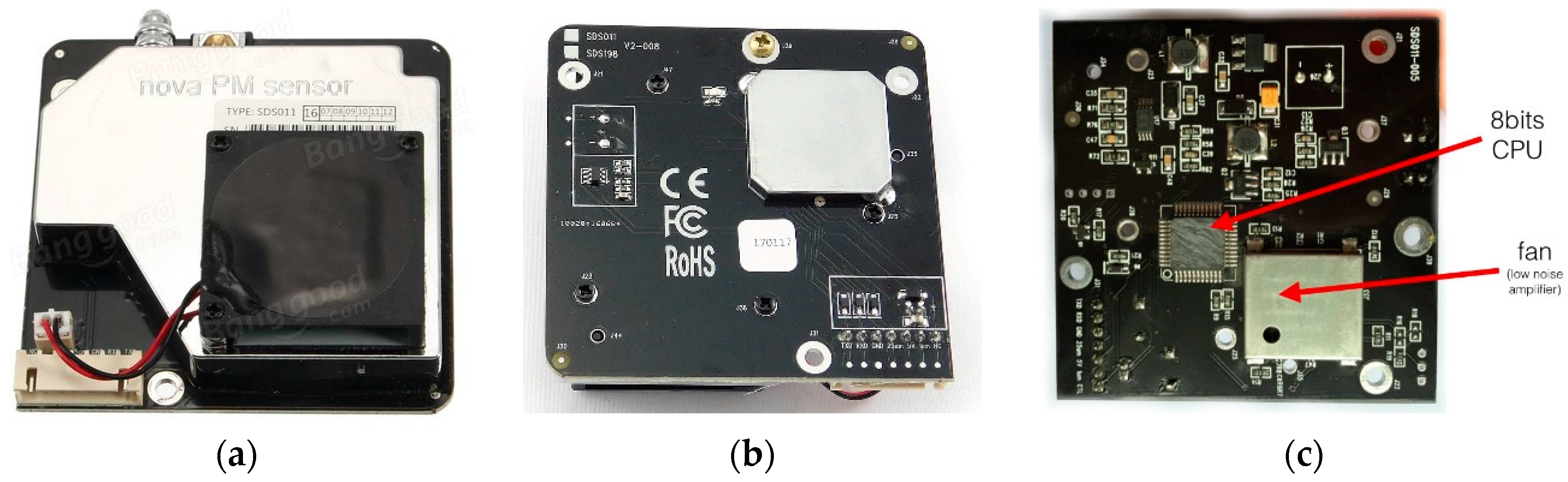
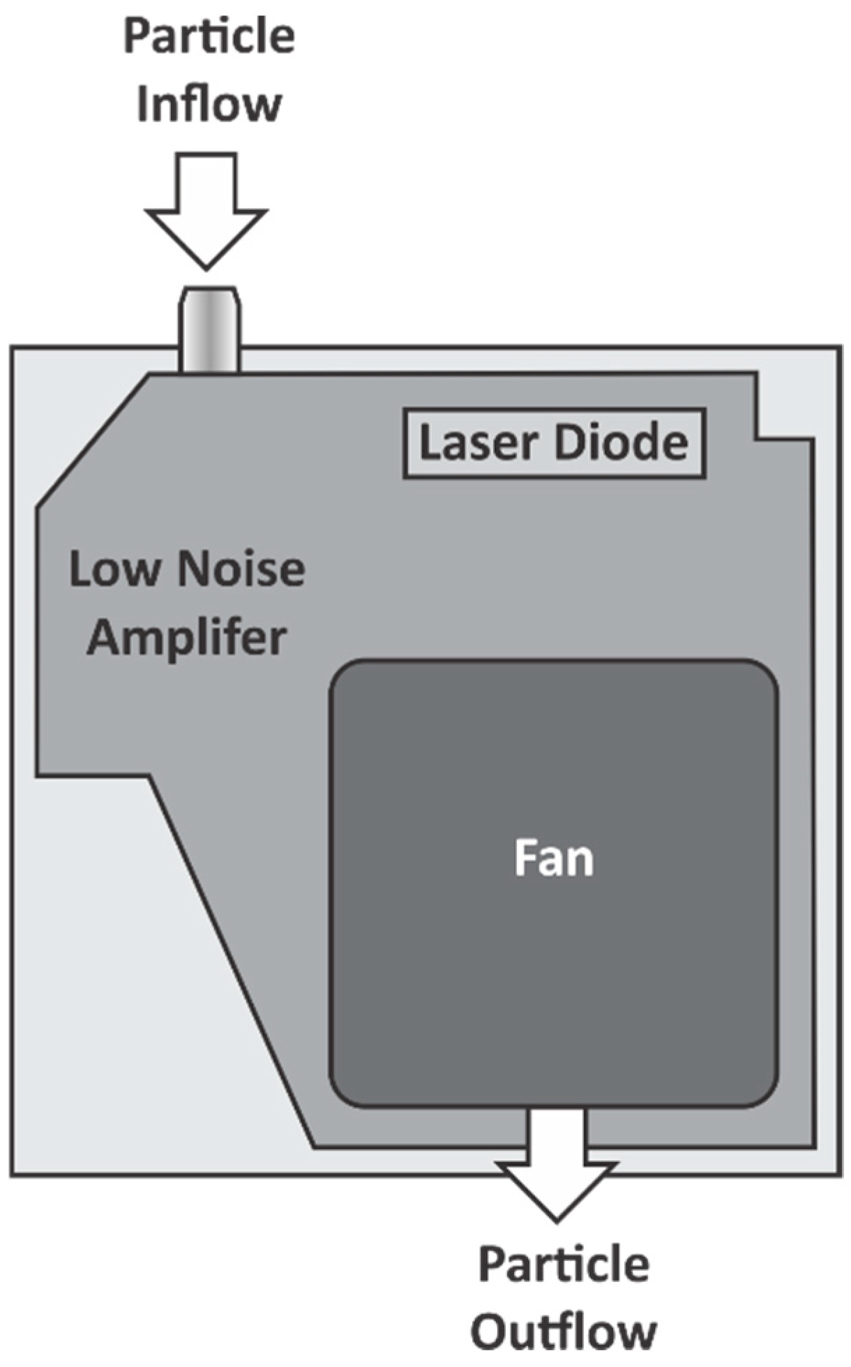
The SDS011 sensor is a quite recent air quality sensor developed by Inovafit, a spin-off from the University of Jinan, Shandong province, P.R. China [17] (Figure 1). The technology is based on laser diffraction theory, where particle density distribution is specified from the light intensity distribution patterns [21,29]. The sensor contains a digital output and a built-in fan (Figure 2), which can measure the particle density distribution between 0.3 to 10 μm in the air. A built-in algorithm convert the particle density distribution into particle mass. A short technical specification of the SDS011 is given in Table 1.
2.2. Sensors Co-Location and Its Measurement Site Description
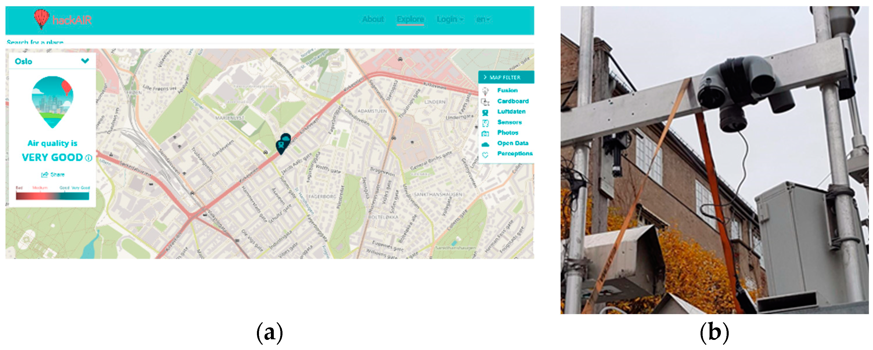
Three SDS011 sensors were co-located at the official air quality monitoring station in Kirkeveien, Oslo, Norway (59°55′56″ N; 10°43′28″ E), which is a road-side station (Figure 3). Road transport is the dominant emission source of PM in the region.
All three sensors were connected with a DHT22 digital temperature and humidity sensor, which measured the relative humidity (RH) and temperature (T) inside the sensor casing. Sensor casing was adopted from luftdaten.info platform [32].
A reference-equivalent instrument TEOM 1405 FDMS (filter dynamics measurement system, which has been calibrated against the true reference Kleinfiltergeraet) is running at the Kirkeveien measurement station. The TEOM 1405FDMS is a TEOM1405DF with an added FDMS unit. The TEOM 1405 DF is a dichotomous analyser. It measures both coarse and fine particles concurrently on two microbalances. In principle, it is two TEOMs in parallel. The inlet airflow is split by a virtual impactor. The FDMS unit compensates for any losses of volatile organic and inorganic compounds on the particles. The inlet air is passed through a drier to avoid condensation. Mass in the dry air is left to accumulate on the filter for 6 min and the mass concentration (MCbase) is measured. Then the dry sample air is diverted through a filter and a chiller at 5 °C to remove all the particles and volatile compounds from the air stream. The clean air is sampled on the filter for another 6 min and the mass concentration (MCref) is measured. The total mass concentration after 12 min is calculated as MC = MCbase − MCref [33]. While the TEOM is not a true reference instrument, the uncertainties resulting of the calibration against the Kleinfiltergeraet are so much smaller than the uncertainties of the SDS011 sensors that they are not likely to show any significant effect on our analysis.
2.3. Data Preparation
PM2.5 data measured by the instrumentation from the official air quality monitoring station was used from 11 December 2017 to 31 March 2018. During this period, one sensor system (S1) using an SD card for data storage recorded data every 30 second, while the other two sensor system (S2 and S3) using the luftdaten.info approach recorded data every 2.5 minutes [32]. PM2.5 mass concentration from each sensor and official monitoring station was provided at hourly time scale.
2.4. Data Analysis
The manufacturer limits the operating range of the SDS011 sensor in terms of RH to 0%–70% (see Table 1). In many countries average RH lies consistently above this threshold for significant periods of the year and as a result the sensors are in practice nonetheless being used somewhat inappropriately by many projects and initiatives outside this range, without taking into account the official operating range. While we are aware of the manufacturer specifications and the physical reasons behind this restriction, we therefore evaluate the performance of the sensors over the entire range of RH, reflecting ongoing practical use of such sensors under real-world conditions. This has the aim of quantifying the uncertainty of the sensors when they are used outside of the official manufacturer-provided operating range for RH. However, we also provide validation results restricted to the manufacturer-provided RH operating range to show the performance of the sensor during appropriate use.
Five performance aspects were examined: operational data coverage of the sensor systems, linearity of the response and accuracy, inter-sensor variability, dependence on air RH and T, and potential accuracy improvement using data calibration with a machine-learning method.
The linearity of response between SDS011 sensors and the official air quality monitoring station was assessed using linear regression, where the data from official air quality monitoring station was the independent variable and the SDS011 sensor data the dependent variable. An R2 value close to 1 reflects a very good linearity of the sensor response in comparison with the official instrumentation. A small R2 value indicates a poor linear relationship.
Accuracy is the degree of closeness between the sensors’ measured values and the reference value. In this context, the long-term averaged data accuracy is here defined as follows [34,35]:
where X is the average concentration measured by the sensors throughout testing period and R is the average concentration measured by the official air quality monitoring station during the testing period. The higher the positive value (percentage), the higher the sensor’s accuracy. For example, a value of 100% implies that sensors measure exactly what the reference instrument measures. In cases where sensors overestimate the reference instrument by more than 100%, sensor accuracy is reported as a negative value, using Equation (1) [34,35].
Inter-sensor variability is related to how close the measurements from three units of the same sensor type are to each other. It is evaluated through a set of descriptive statistical parameters, such as mean, range, and standard deviation. For a set of three sensors the inter-sensor variability is reported as a percentage and is calculated as follows [34,35]:
where Mean-highest is the highest of the three sensors’ average concentrations, Mean-lowest is the lowest of the three sensors’ average concentrations, and Mean-average is the average of the three sensors’ average concentrations.
The impact of RH and T on the sensor response was tested by analysing the relationship between observed PM2.5 sensor error (measured as sensor observation data minus reference data) and air temperature as well as RH for three sensors. A Loess fit [36] was used to better illustrate the relationship.
Multiple-linear regression (MLR) [37] and a machine learning method (Random Forest) [38] were used for illustrating potential sensor data accuracy improvement by correcting for the effects of RH and T measured by DHT22 sensor, which was located right beside the SDS011 sensor within same sensor casing.
All data analyses were carried out in the R environment for statistical computing and visualization [39].
3. Results and Discussion
3.1. Sensors and Reference Instrument Operational Data Coverage
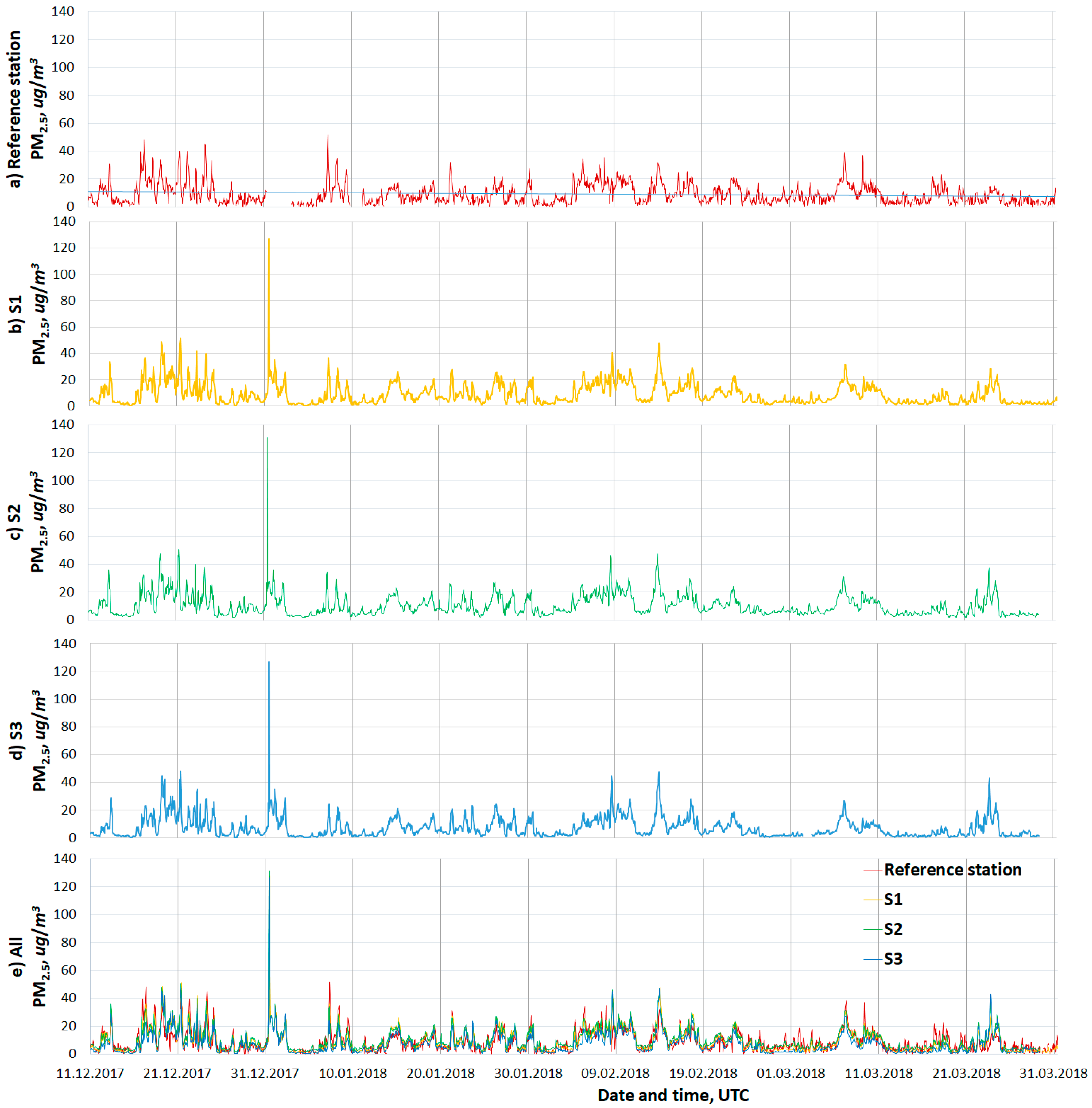
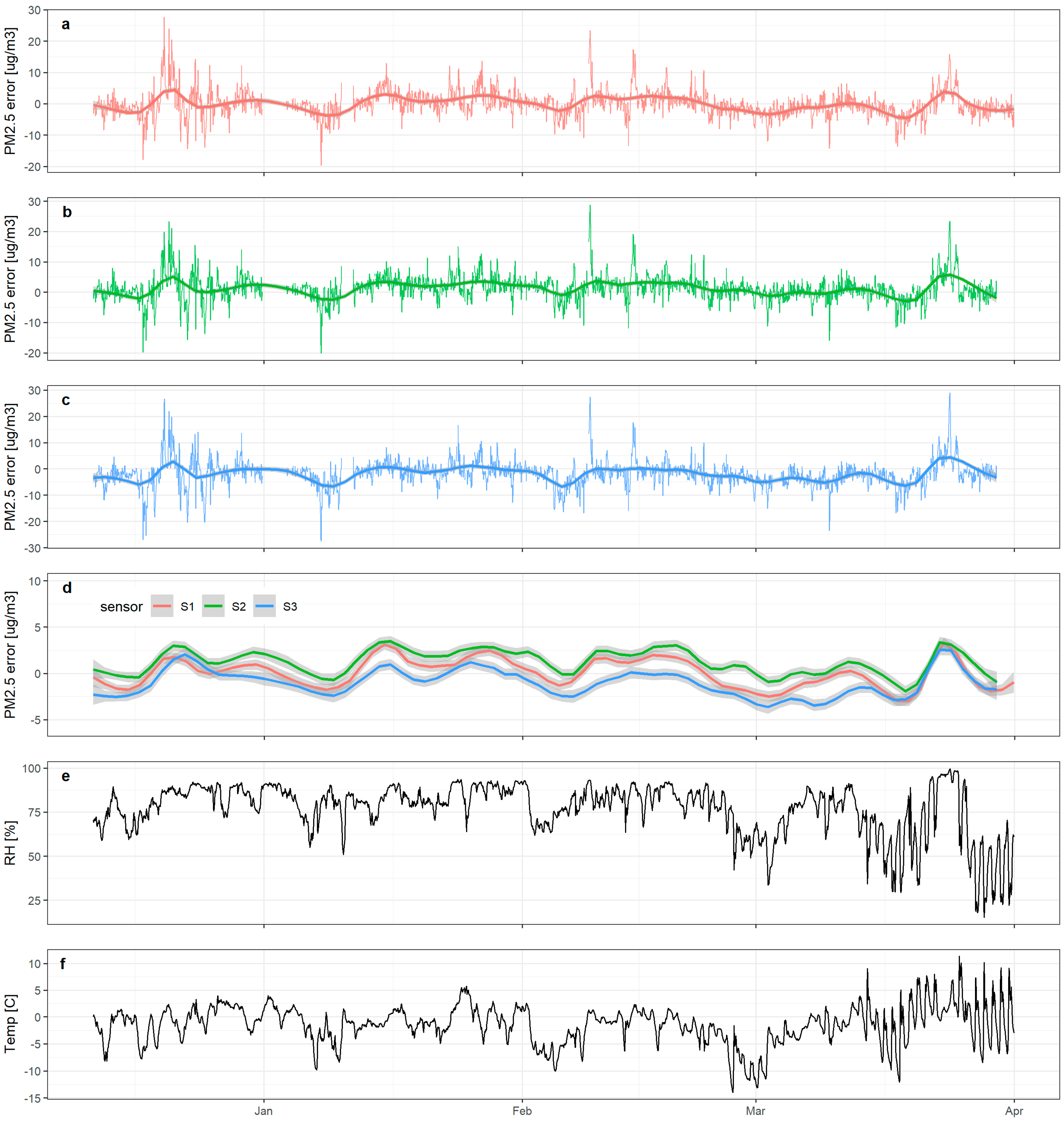
Figure 4 presents the results of PM2.5 measurements for the period of nearly four-month from three SDS011 sensors and official reference monitoring station, respectively, at hourly time scale. Data gaps (i.e., from 31 December 2017 to 3 March 2018) for the reference monitoring station were related to official reference-equivalent instrument error (e.g., power outages and maintenance activities) (Figure 4a). Data gaps for S2 and S3 (i.e., 3 March 2018 for S3, 30 March 2018 to 31 March 2018 for both S2 and S3) were due to platform error (Figure 4c, d). In general, the operation of the tested three SDS011 PM sensors was quite stable all near four-month study, and no obvious sensor errors have been observed (Figure 4e). Episodes of elevated PM2.5 concentrations were observed during the new-year eve within the time-period of 23:00 p.m., 31 December 2017 to 01:00 a.m., 1 January 2018. This is clearly connected to particle emissions from the fireworks (Figure 4b–e).
All measurements were conducted under varying meteorological conditions. Figure 5 illustrates that the PM2.5 data from three sensors follow similar patterns near four-month period, thus indicating that they respond similarly to varying environmental conditions. Qualitatively no significant drift of the signal was observed for any of the three sensor systems over the study period. The PM2.5 concentrations at hourly time scale ranged from 0.4 μg/m3 to 127.5 μg/m3. The T range the sensor systems were exposed to was −14.0–+11.4 °C, and the RH range was 15.4–+99.5%, respectively (Figure 5). The operation of the three tested SDS011 sensors was stable throughout the almost four-month study period and was no obvious errors in terms of data availability or failures of electronic parts of the sensors were observed within these meteorological conditions.
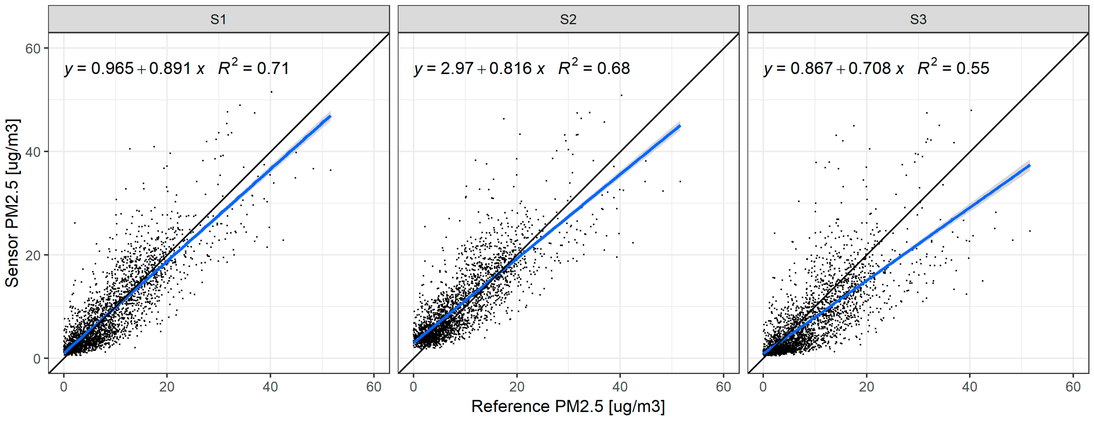
3.2. Linearity of the Response and Accuracy
Data from three SDS011 sensor systems was compared with data generated from the official air quality monitoring station over a nearly four-month period (11 December 2017–31 March 2018) (Figure 6, Table 2). The results show that the PM sensors provided a consistent measurement response to measurements of the reference monitoring station. Three sensors demonstrated a substantial degree of correlation against the official reference instrument from air quality monitoring station, with R2 values equal to 0.71 (S1), 0.68 (S2), and 0.55 (S3), respectively. This result is consistent with the similar study implemented in Wroclaw, Poland by Badura et al. 2018 [30]. As can be seen in Table 2, the slope of all three regression models is slightly below 1, indicating a general under-estimation of the PM2.5 mass for all three units, particularly for higher pollution levels. Furthermore, the mean error is generally below 2 μg/m3 and the RMSE (Root-Mean-Square Error) is less than 6 μg/m3 for all three units. Sensor system S3 shows the overall worst performance of all three units.
The three sensors demonstrated satisfactory to comparatively high data accuracy of the long-term mean concentration with values of 98.16%, 86.82% and 80.76%, respectively (Table 3). The long-term averaged data accuracy for three sensors reached 88.58%.
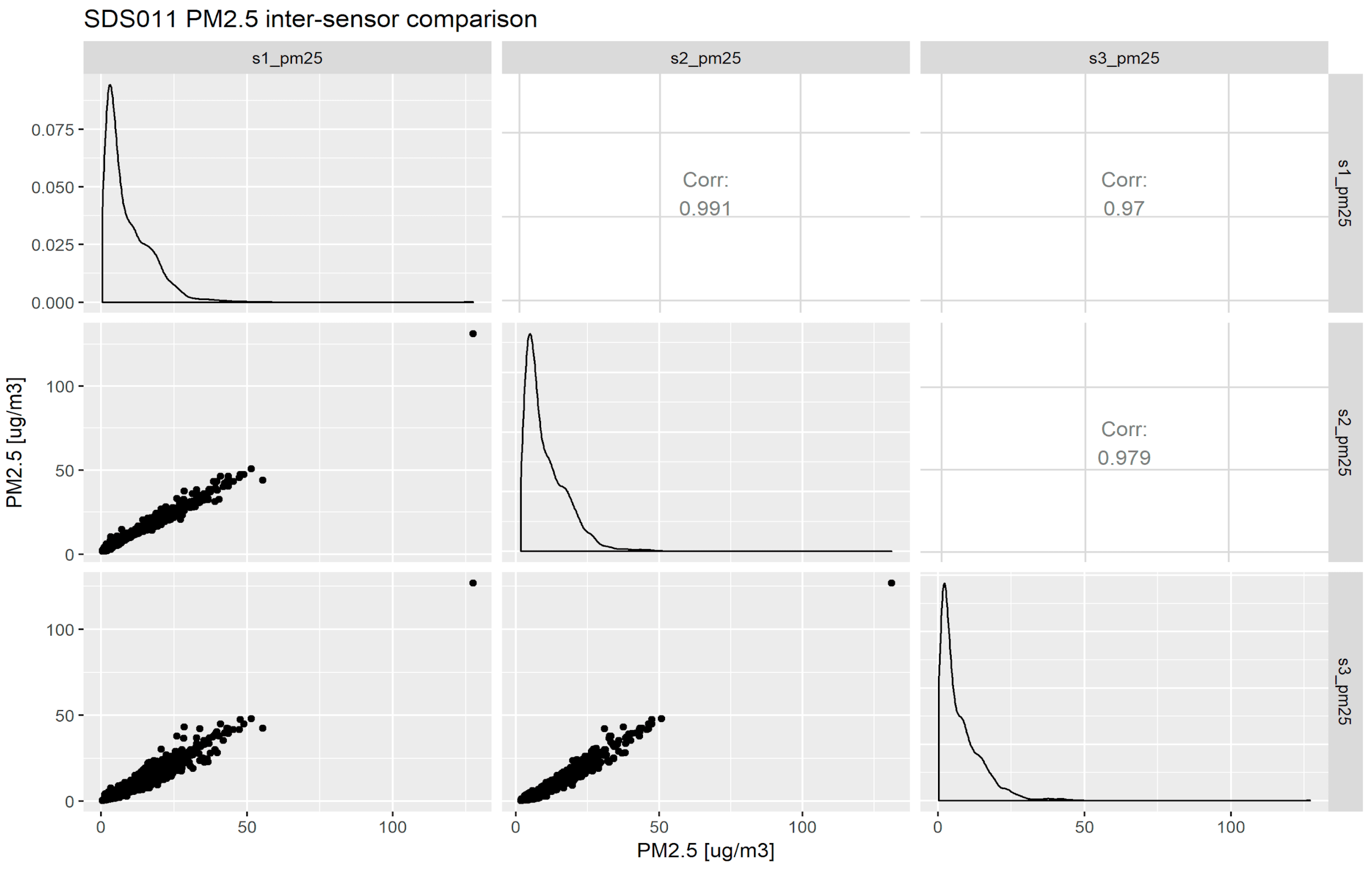
3.3. Intersensor Variability
The inter-sensor variability over the almost four-month study period (11 December 2017–31 March 2018) was analysed. We can see that three sensors provide quite similar results and do not vary substantially (Figure 4, Table 4, Figure 7), with inter-model variability around 9.64%, which calculated as following:
Figure 7 visualizes inter-sensor variability for three SDS011 sensors as a scatterplot matrix with inter-sensor correlations exhibiting R values higher than 0.97.
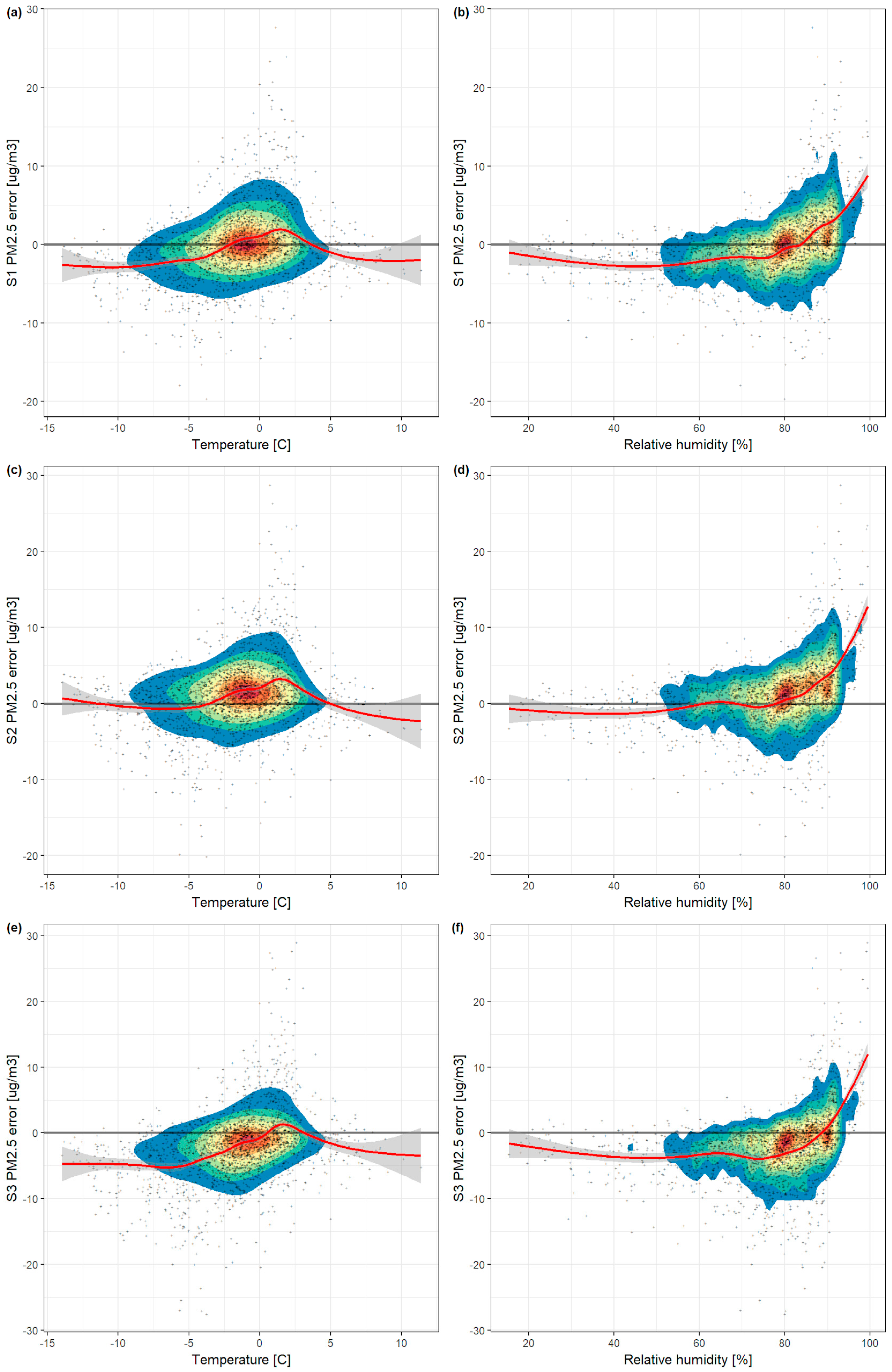
3.4. Influence of Relative Humidity and Air Temperature
Sensors were exposed to T in the range of −14.0–+11.4 °C, and RH in the range of about 15.4–+99.5%. These parameters were measured by the DHT22 sensor located beside the SDS011 sensor, within same sensor casing. Therefore, measurements of T and RH are independent and not affected by the data availability of sensors or electronic parts of sensors.
Most low-cost sensors for air quality, including such as Alphasense OPC-N2 [23,30], Plantower PMS7003 [19,20,30], and Nova SDS011 [21,30], are to some extent influenced by the ambient environmental conditions. Therefore, we explored the relationship between the observed PM2.5 error as a function of T and RH (Figure 8).
Figure 8 shows how the PM2.5 sensor error (calculated as the hourly mean sensor observation minus the hourly mean observations from the TEOM instrument) varies with T and RH. While all of the raw hourly data the overall patterns can be most easily observed by analysing the red line which represent a Loess fit [40] to the raw data.
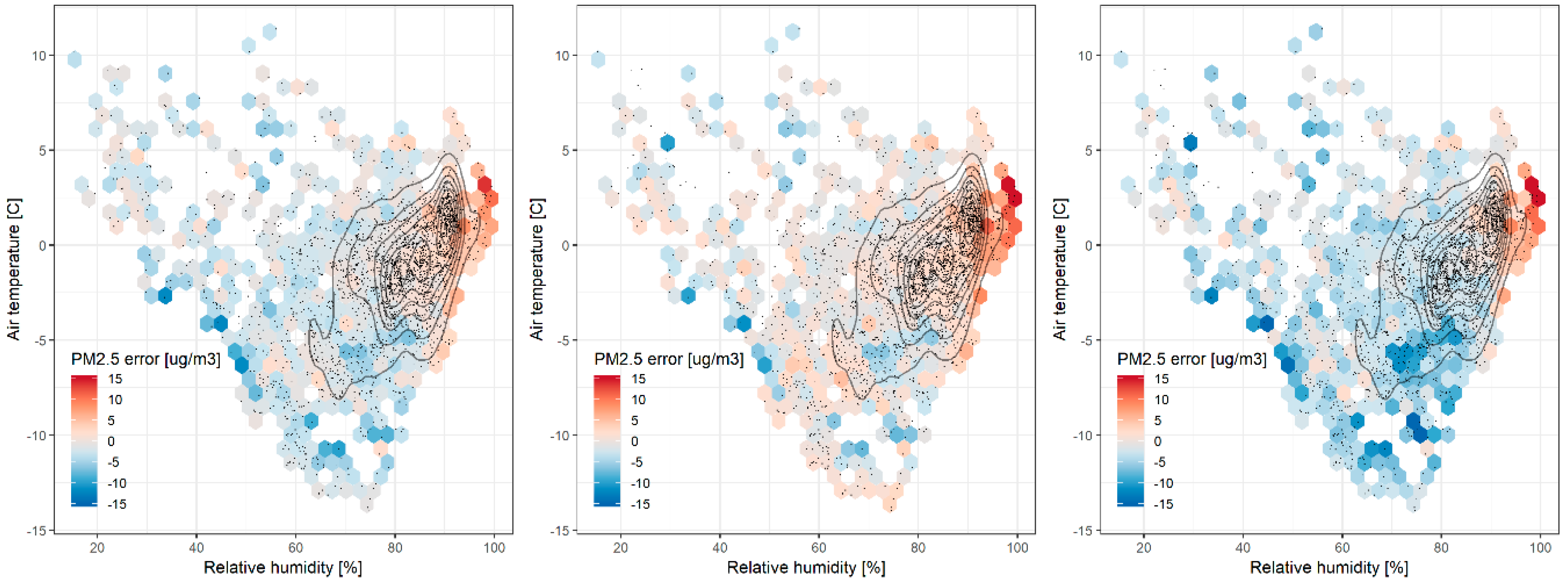
As for the dependence of the PM2.5 sensor error with air T, all three units show similar patterns. For relatively low T under −5 °C the errors were either slightly negative on average (S1 and S3) or close to zero (S2). For T around zero degrees, all three units show slightly positive errors between 0 μg/m3 and 5 μg/m3. For higher T the average PM2.5 of all three units decreases again. There is no obvious physical reason for this pattern and we think that this peak at around zero degrees is rather related to high RH values at these temperatures (see also Figure 9).
In terms of the impact of RH on the PM2.5 sensor errors, we can initially observe that there is a similar behaviour for all three units. The errors tend to be quite stable between −5 μg/m3 and 0 μg/m3 for RH levels less than approximately 80%. However, for RH values between 80% and 100% we can see a substantial increase in PM2.5 error for all three units. At close to 100% RH, all three units show positive PM2.5 errors of 10 μg/m3 to 15 μg/m3 on average. While the RH values that occurred during our study period ranged from a low of 15% to nearly 100%, the highest frequency of RH values in this study was found in two clusters of around 80% and 90%, respectively.
In order to better disentangle the effects of T and RH, Figure 9 shows the PM2.5 error of each sensor as a function of both RH and air T at the same time. The most obvious pattern is the substantial cluster of positive errors for high RH (>90%) at T above 0 °C. This pattern exists for all three units, although there are some slight differences in the magnitude of the errors. We can further observe the largest negative errors for low T (<−5 °C) and RH between approximately 40% and 80%. The errors tend to decrease again slightly for even lower T (<−13 °C) but the range of RH is very small in this case and the overall number of samples is very low, making it difficult to draw further conclusions. The effect of RH and T on sensors’ data quality needs to be taken into consideration when using low-cost particle sensors [41,42].
There could be several reasons for the effect of RH on the sensor performance. The most obvious reason is that the low-cost sensor has no system for drying the particles before they enter the optical chamber, which means that aerosol particles as well as fog droplets are counted. This leads to a positive artefact compared to the TEOM. The second reason is particle growth by water vapour condensation. Depending on the chemical composition of the particles, water vapour can condense onto the particle and particles grow by condensation. This growth in particle diameter is reflected by the radius to the power of three in the particle mass and would also lead to a positive artefact compared to the TEOM, as the TEOM measures dry particles. The third reason is the change of optical properties of particles measured if water condensation occurs onto the particle. A critical parameter when calculating the particle density distribution is the refractive index of the particles. Water vapour condensation changes the imaginary component in the Mie equation. This is the extinction coefficient of the material, defined as the reduction of transmission of optical radiation caused by absorption and scattering of light, leading to a wrong estimation of the size and therefore the mass reported by the instrument.
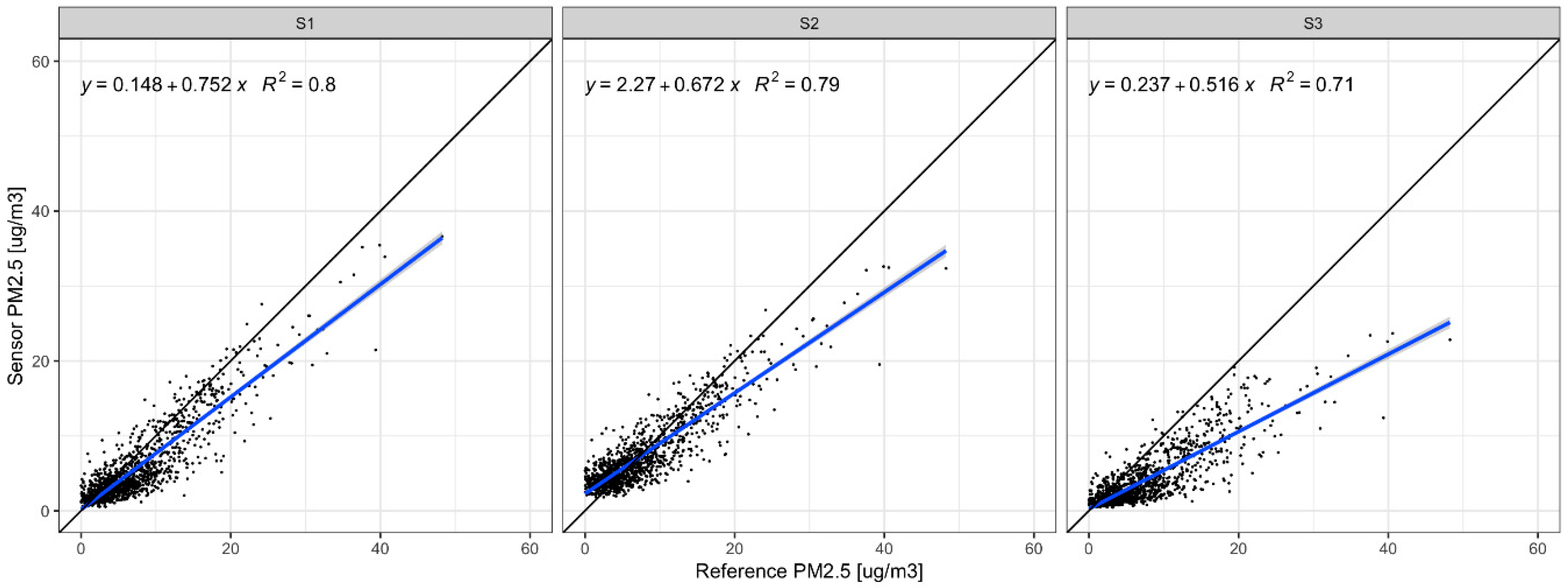
Based upon these observations of high RH negatively affecting the sensors’ response, we filtered sensor data with RH less than 80%, and plotted it against officially measured concentrations of PM2.5 (Figure 10). The results indicate that the three sensors demonstrated an increased degree of correlation against the official reference instrument from air quality monitoring station (Figure 6), with R2 values increased from 0.71 to 0.80 (S1), 0.68 to 0.79 (S2), and 0.55 to 0.71 (S3), respectively. However, the slope of the regression lines is slightly lower than before for all three units (Figure 6).
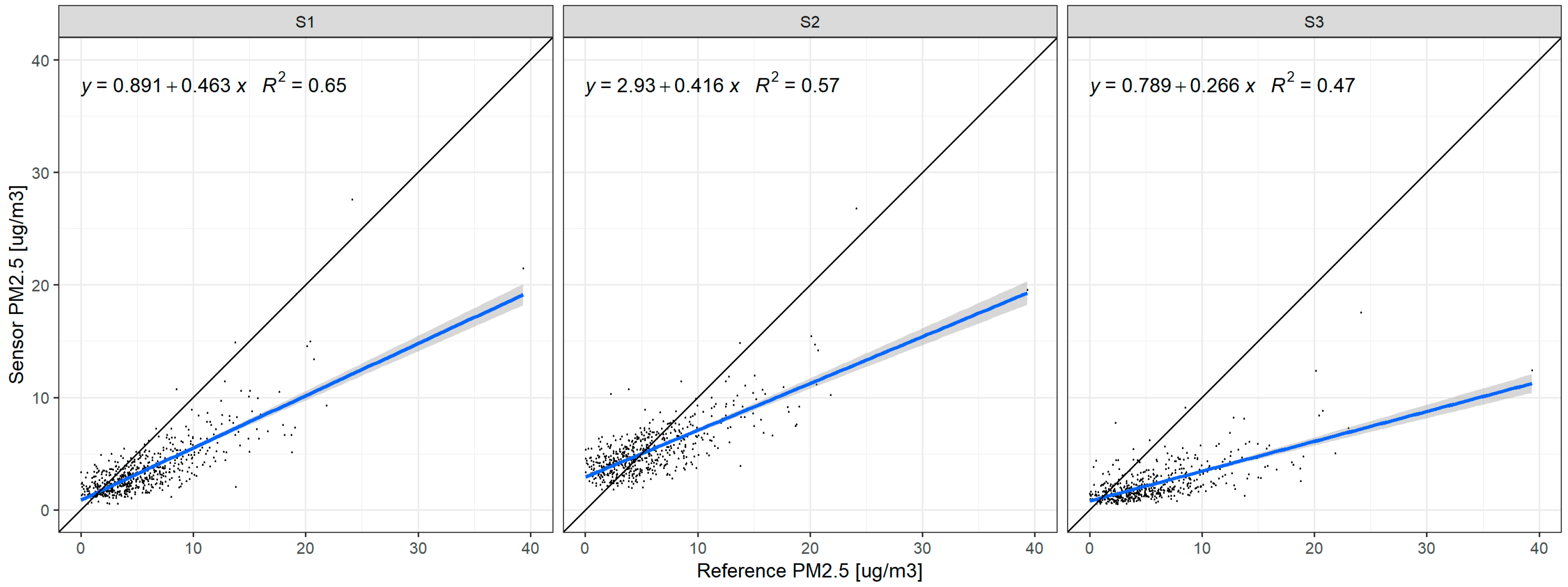
Furthermore, we filtered sensor data with RH less than 70% which aligned with the manufacturer-provided RH operating range (max. RH 70%), and plotted it against officially measured concentrations of PM2.5 (Figure 11). The results showed that three sensors demonstrated a decreased degree of correlation against the official reference instrument from air quality monitoring station, with R2 values decreased from 0.71 to 0.65 (S1), 0.68 to 0.57 (S2), and 0.55 to 0.47 (S3), respectively. The physical reason for these decreased correlation is not entirely clear, but it may be related to the fact that nearly 60% of the data were filtered out. Since this filtering also includes most observations at concentration of greater than 20 μg/m3, the available range of concentrations is decreased significantly, which could be responsible for a decrease in correlation.
3.5. Correction for Temperature and Humidity Effects
It is to some extent possible to statistically correct for the effects of RH and T that were shown in the previous section, although such corrections tend to be specific to the location at which the co-location is being carried out and cannot easily be transferred to other locations with different conditions. We demonstrate an example for such a correction procedure here using simple multilinear regression (MLR) [37] and a random forest (RF) model [38].
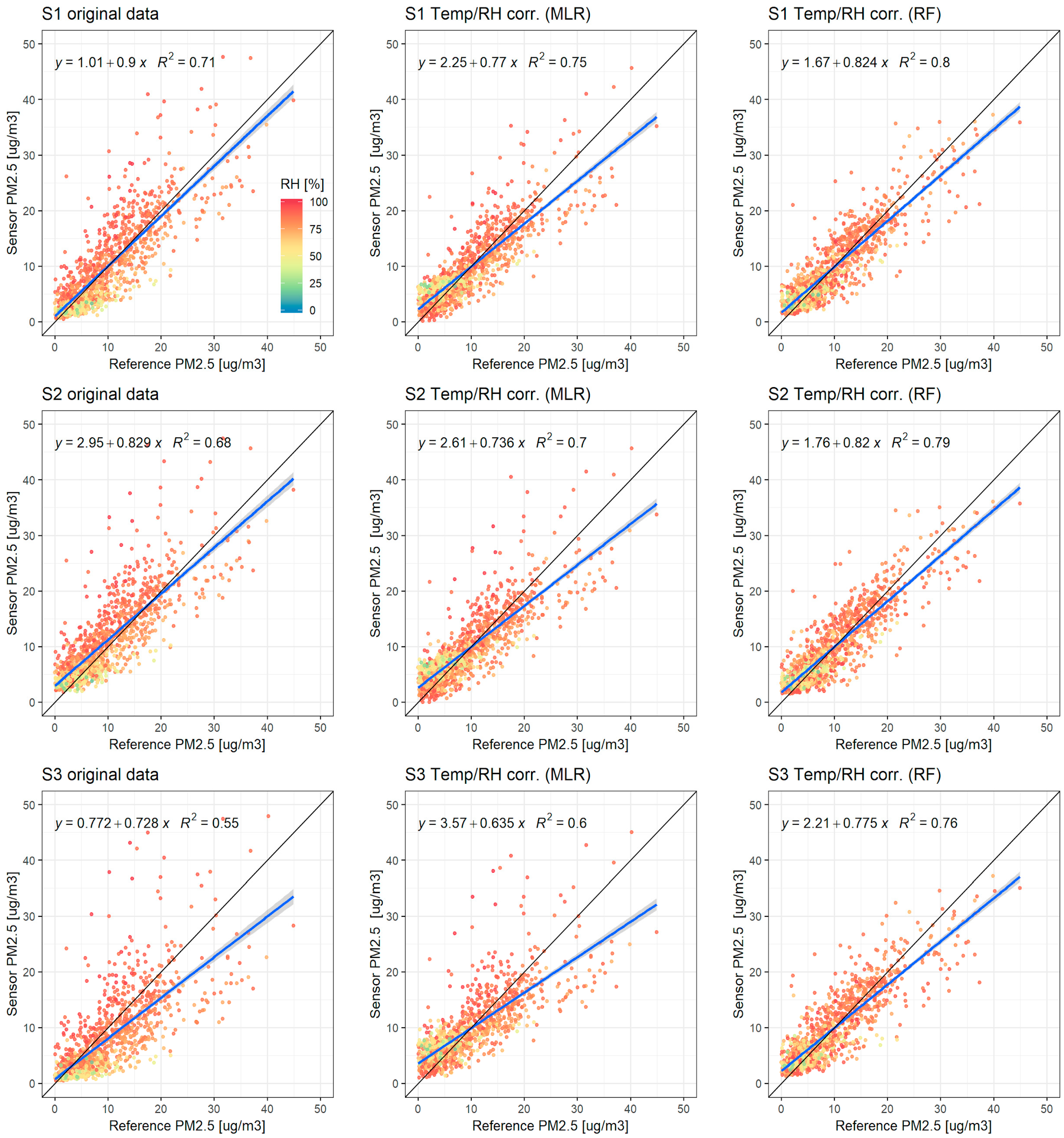
Figure 12 shows the improvement in sensor accuracy that can be achieved when RH and T are accounted for as part of the calibration. The left column of Figure 12 shows the original out-of-sensor data for all three sensors, whereas the middle column and the right column show the data after calibration using a MLR and a RF model, respectively. It can be seen that already a simple linear regression can improve the accuracy with respect to reference data somewhat, although the increases in R2 value are relatively modest. However, using the same dataset with a RF model increases the correlation significantly, explaining roughly 10% more of the variability for sensors S1 and S2 and even 20% more of the variability in the case of sensor S3, with R2 value increased from 0.71 to 0.80, from 0.68 to 0.79, from 0.55 to 0.76, respectively (Figure 12).
It should be noted that this correction for the effect of air T and RH is only valid for the particular location at which the model was trained. As such, the model is dependent on both the specific characteristics of the environmental parameters at this site but also of the characteristics of the PM that occurs at this site (e.g., particle type, size, etc.). Applying such a correction model at a different location that has either different environmental conditions or different particle characteristics is likely to result in inferior performance.
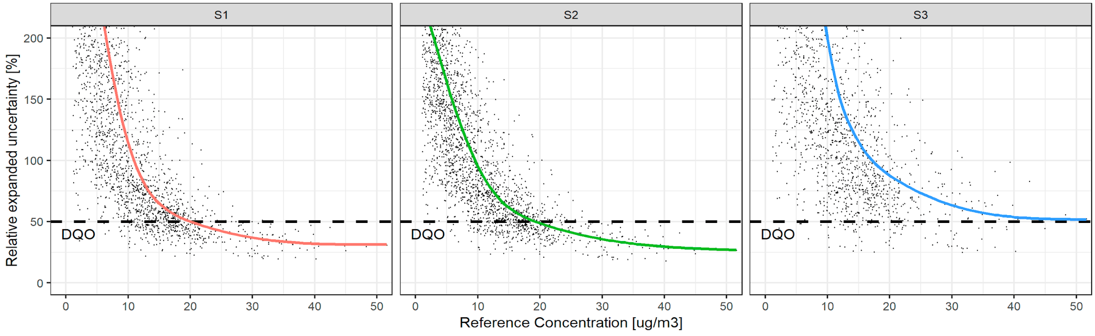
Figure 13 shows scatter plots of the relative expanded uncertainty as a function of the PM2.5 concentration measured at the air quality monitoring station, following the methodology described by Spinelle et al. (2015) [43]. Based on these plots, two out of the three units (S1 and S2) reach the data quality objective (DQO) of 50% as defined in the European Air Quality Directive [8]. Both sensors reach relative expanded uncertainties [44,45] of below 50% approximately at concentrations of 20 μg/m3. S3, however, does not meet the DQO.
4. Conclusions
The conducted comparison of three SDS011 sensors with data from an official reference air quality monitoring station demonstrated that the SDS011 sensor generally follow the PM2.5 variability. Linear regression indicated a good correlation between the two datasets with R2 values equal to 0.71 (S1), 0.68 (S2) and 0.55 (S3), respectively, over almost four-month period in challenging, Norwegian winter conditions with frequently high relative humidity. The inter-sensor variability analysis showed that the three sensors provided quite similar results and did not vary substantially from each other, with inter-model variability around 9.64%, and inter-sensor correlations R values higher than 0.97. RH and, to a very small extent, T affect the SDS011 performance. Particularly high RH values (over 80%) cause significant overestimates of the true PM2.5 mass. While the sensors provide generally reasonable estimates of PM2.5 mass out-of-the-box, our results also indicate that a field calibration under representative environmental conditions is highly beneficial for improving the accuracy of the measurements. This study was limited to a relatively low number of months with limited variation in environmental conditions. To cover a wider range of meteorological conditions and to test the long-term stability of the sensors, we are working on a follow-up study that will evaluate the performance of the sensors using a yearlong time series at least and sensors located in a wide variety of differing environmental conditions and pollution regimes.
Despite the reasonably good performance of these sensors, it should be noted that the potential misuse of these sensors is nonetheless high, especially when they are used outside of a research environment for citizen science applications and personal air quality monitoring, where the users might not have the required knowledge to adequately judge the uncertainty of the sensors. In such cases, the deployment of these sensors will almost certainly not be confined to environments with RH < 80%, and there is no specific notification to the users that the readings are unreliable when the RH is > 80%, although the manufacturer provides a recommended RH operating range. In addition, the relative uncertainties can be quite high for hourly values, and users should be aware of this limitation and take caution in interpreting such measurements. Nevertheless, considering their very low cost and the performance assessment results overall, we conclude that the SDS011 has significant potential for implementing a dense monitoring network when the environmental conditions exhibit on average relatively low relative humidity (RH < 80%). When used under environmental conditions that often exhibit high relative humidity, appropriate automated filtering or correction routines need to be established to remove problematic observations from the datasets or at minimum provide the users with clear indications of the estimated observations uncertainty. If these conditions are met, we conclude that networks of SDS011 sensors could in future, for example, complement the regulatory outdoor air quality monitoring networks and improve the spatial and temporal resolution of PM2.5 data, opening up various applications for the research community, regulatory agencies and raising public awareness.
Author Contributions
H.-Y.L. and R.H. designed and performed the field experiments; P.S. and H.-Y.L. analysed the data; M.V. contributed to results interpretation by explaining the dependence of T and RH on sensors’ response; H.-Y.L. and P.S. wrote the paper.
Funding
The research leading to these results has received funding from EU H2020 project hackAIR with contract no. 688363 (www.hackair.eu).
Acknowledgments
The authors thank Peter Schild from Oslo and Akershus University College and his EPS students for providing the Arduino SD card code for testing. We would like to thank the anonymous referees for their very valuable comments.
Conflicts of Interest
The authors declare no conflict of interest.
References
- European Environmental Agency (EEA). Air Quality in Europe—2017 Report; Publications Office of the European Union: Luxembourg, 2017; pp. 30–65. ISBN 978-92-9213-920-9. [Google Scholar]
- Liu, H.-Y.; Dunea, D.; Iordache, S.; Pohoata, A. A Review of Airborne Particulate Matter Effects on Young Children’s Respiratory Symptoms and Diseases. Atmosphere 2018, 9, 150. [Google Scholar] [CrossRef]
- Liu, H.-Y.; Bartonova, A.; Schindler, M.; Sharma, M.; Behera, S.N.; Katiyar, K.; Dikshit, O. Respiratory Disease in Relation to Outdoor Air Pollution in Kanpur, India. Arch. Environ. Occup. Health 2013, 68, 204–217. [Google Scholar] [CrossRef] [PubMed]
- Dockery, D.W.; Stone, P.H. Cardiovascular risks from fine particulate air pollution. N. Engl. J. Med. 2007, 356, 511–513. [Google Scholar] [CrossRef] [PubMed]
- Pérez, L.; Medina-Ramón, M.; Künzli, N.; Alastuey, A.; Pey, J.; Pérez, N.; García, R.; Tobías, A.; Querol, X.; Sunyer, J. Size fractionate particulate matter, vehicle traffic, and case-specific daily mortality in Barcelona (Spain). Environ. Sci. Technol. 2009, 43, 4707–4714. [Google Scholar] [CrossRef] [PubMed]
- IARC: Outdoor Air Pollution a Leading Environmental Cause of Cancer Deaths. Available online: https://www.iarc.fr/en/media-centre/iarcnews/pdf/pr221_E.pdf (accessed on 5 April 2018).
- EEA: Europe Air Pollution Causes 467,000 Early Deaths a Year: Report. Available online: https://phys.org/news/2016-11-europe-air-pollution-early-deaths.html (accessed on 7 May 2018).
- Directive 2008/50/EC of the European Parliament and the Council of 21 May 2008 on Ambient Air Quality and Cleaner Air for Europe. Available online: https://eur-lex.europa.eu/legal-content/en/ALL/?uri=CELEX:32008L0050 (accessed on 16 October 2018).
- Breslow, N.E.; Lin, X. Bias correction in generalised linear mixed models with a single component of dispersion. Biometrika 1995, 82, 81–91. [Google Scholar] [CrossRef]
- Gibson, M.D.; Kundu, S.; Satish, M. Dispersion model evaluation of PM2.5, NOx and SO2 from point and major line sources in Nova Scotia, Canada using AERMOD Gaussian plume air dispersion model. Atmos. Pollut. Res. 2013, 4, 157–167. [Google Scholar] [CrossRef]
- Schneider, P.; Castell, N.; Vogt, M.; Dauge, F.R.; Lahoz, W.A.; Bartonova, A. Mapping urban air quality in near real-time using observations from low-cost sensors and model information. Environ. Int. 2017, 106, 234–247. [Google Scholar] [CrossRef]
- Schneider, P.; Castell, N.; Dauge, F.R.; Vogt, M.; Lahoz, W.A.; Bartonova, A. A Network of Low-Cost Air Quality Sensors and Its Use for Mapping Urban Air Quality. In Mobile Information Systems Leveraging Volunteered Geographic Information for Earth Observation; Bordogna, G., Carrara, P., Eds.; Springer International Publishing: Cham, Switzerland, 2017; Volume 4, pp. 93–110. ISBN 978-3-319-70878-2. [Google Scholar]
- Castell, N.; Schneider, P.; Grossberndt, S.; Fredriksen, M.F.; Sousa-Santos, G.; Vogt, M.; Bartonova, A. Localized real-time information on outdoor air quality at kindergartens in Oslo, Norway using low-cost sensor nodes. Environ. Res. 2018, 165, 410–419. [Google Scholar] [CrossRef]
- Castell, N.; Dauge, F.R.; Schneider, P.; Vogt, M.; Lerner, U.; Fishbain, B.; Broday, D.; Bartonova, A. Can commercial low-cost sensor platforms contribute to air quality monitoring and exposure estimates? Environ. Int. 2017, 99, 293–302. [Google Scholar] [CrossRef]
- Liu, H.-Y.; Skjetne, E.; Kobernus, M. Mobile phone tracking: In support of modelling traffic-related air pollution contribution to individual exposure and its implications for public health impact assessment. Environ. Health 2013, 12, 93. [Google Scholar] [CrossRef]
- Skjetne, E.; Liu, H.-Y. Traffic maps and smartphone trajectories to model air pollution, exposure and health impact. J. Environ. Prot. 2017, 8, 1372–1392. [Google Scholar] [CrossRef]
- GP2Y1010AU0F: Compact Optical Dust Sensor. Available online: https://www.sparkfun.com/datasheets/Sensors/gp2y1010au_e.pdf (accessed on 21 May 2018).
- Shinyei PPD42 Particle Sensor. Available online: https://github.com/mozilla-sensorweb/sensorweb-wiki/wiki/Shinyei-PPD42-Particle-Sensor (accessed on 21 May 2018).
- Digital Universal Particle Concentration Sensor. Available online: http://www.aqmd.gov/docs/default-source/aq-spec/resources-page/plantower-pms1003-manual_v2-5.pdf (accessed on 21 May 2018).
- PA-II Dual Laser Air Quality Sensor. Available online: https://www.purpleair.com/sensors (accessed on 21 May 2018).
- Laser PM2.5 Sensor Specification Product Model: SDS011, Version: V1.3. Available online: https://nettigo.pl/attachments/398 (accessed on 21 May 2018).
- AirBeam Technical Specifications, Operation & Performance. Available online: http://www.takingspace.org/airbeam-technical-specifications-operation-performance/ (accessed on 22 May 2018).
- Alphasense Air Sensors for Air Quality Networks—Particulates. Available online: http://www.alphasense.com/index.php/products/optical-particle-counter/ (accessed on 22 May 2018).
- Wuhan Cubic Optoelectronics Co., Ltd. Dust Sensor for Automotive Applications PM3007. Available online: http://www.directindustry.com/prod/wuhan-cubic-optoelectronics-co-ltd/product-54752-1844530.html (accessed on 17 October 2018).
- Hahn, D.W. Light Scattering Theory; University of Florida: Gainesville, FL, USA, 2009. [Google Scholar]
- Zikova, N.; Masiol, M.; Chalupa, D.C.; Rich, D.Q.; Ferro, A.R.; Hopke, P.K. Estimating Hourly Concentrations of PM2.5 across a Metropolitan Area Using Low-Cost Particle Monitors. Sensors 2017, 17, 1922. [Google Scholar] [CrossRef] [PubMed]
- Mukherjee, A.; Stanton, L.G.; Graham, A.R.; Roberts, P.T. Assessing the utility of low-cost particulate matter sensors over a 12-week period in the Guyama Valley of California. Sensors 2017, 17, 1805. [Google Scholar] [CrossRef]
- Zheng, T.; Bergin, M.H.; Johnson, K.K.; Tripathi, S.N.; Shirodkar, S.; Landis, M.S.; Sutaria, R.; Carlson, D.E. Field evaluation of low-cost particulate matter sensors in high and low concentration environments. Atmos. Meas. Tech. 2018, 11, 4823–4846. [Google Scholar] [CrossRef]
- Genikomsakis, K.N.; Galatoulas, F.K.; Dallas, P.I.; Ibarra, L.M.C.; Margaritis, D.; Ioakimidis, C. Development and On-Field Testing of Low-Cost Portable System for Monitoring PM2.5 Concentrations. Sensors 2018, 18, 1056. [Google Scholar] [CrossRef] [PubMed]
- Badura, M.; Batog, P.; Drzeniecka-Osiadacz, A.; Modzel, P. Evaluation of Low-Cost Sensors for Ambient PM2.5 Monitoring. J. Sens. 2018, 2018, 5096540. [Google Scholar] [CrossRef]
- Kosmidis, E.; Syropoulou, P.; Tekes, S.; Schneider, P.; Spyromitros-Xioufis, E.; Riga, M.; Charitidis, P.; Moumtzidou, A.; Papadopoulos, S.; Vrochidis, S.; et al. hackAIR: Towards Raising Awareness about Air Quality in Europe by Developing a Collective Online Platform. ISPRS Int. J. Geo-Inf. 2018, 7, 187. [Google Scholar] [CrossRef]
- Measure Air Quality Yourself. Available online: https://luftdaten.info/en/home-en/ (accessed on 21 May 2018).
- Thermo Scientific™—1405-F TEOM™ Continuous Air Monitor. Available online: https://www.thermofisher.com/order/catalog/product/TEOM1405F (accessed on 22 June 2018).
- Polidori, A.; Papapostolou, V.; Zhang, H. Laboratory Evaluation of Low-Cost Air Quality Sensors—Laboratory Setup and Testing Protocol. Available online: http://www.aqmd.gov/docs/default-source/aq-spec/protocols/sensors-lab-testing-protocol6087afefc2b66f27bf6fff00004a91a9.pdf (accessed on 13 December 2018).
- Papapostolou, V.; Zhang, H.; Feenstra, B.J.; Polidori, A. Development of an environmental chamber for evaluating the performance of low-cost air quality sensors under controlled conditions. Atmos. Environ. 2017, 171, 82–90. [Google Scholar] [CrossRef]
- Cleveland, W.S.; Devlin, S.J. Locally Weighted Regression: An Approach to Regression Analysis by Local Fitting. J. Am. Stat. Assoc. 1988, 83, 596–610. [Google Scholar] [CrossRef]
- Freedman, D.A. Statistical Models: Theory and Practice, 1st ed.; Cambridge University Press: Cambridge, UK, 2009; p. 26. ISBN 978-0-521-74385-3. [Google Scholar]
- Ho, T.K. Random Decision Forests. In Proceedings of the 3rd International Conference on Document Analysis and Recognition, Montreal, QC, Canada, 14–16 August 1995; pp. 278–282. [Google Scholar]
- The R Project for Statistical Computing. Available online: https://www.r-project.org/ (accessed on 21 May 2018).
- Cleveland, W.S. Robust Locally Weighted Regression and Smoothing Scatterplots. J. Am. Stat. Assoc. 1979, 74, 829–836. [Google Scholar] [CrossRef]
- Jayaratne, R.; Liu, X.; Thai, P.; Dunbabin, M.; Morawska, L. The influence of humidity on the performance of a low-cost air particle mass sensor and the effect of atmospheric fog. Atmos. Meas. Tech. 2018, 11, 4883–4890. [Google Scholar] [CrossRef]
- Hojaiji, H.; Kalantarian, H.; Bui, A.A.T.; King, C.E.; Sarrafzadeh, M. Temperature and Humidity Calibration of a Low-Cost Wireless Dust Sensor for Real-Time Monitoring. In Proceedings of the 2017 IEEE Sensors Applications Symposium (SAS), Glassboro, NJ, USA, 13–15 March 2017. [Google Scholar]
- Spinelle, L.; Gerboles, M.; Gabriella Villani, M.; Aleixandre, M.; Bonavitacola, F. Field calibration of a cluster of low-cost available sensors for air quality monitoring. Part A: Ozone and nitrogen dioxide. Sens. Actuators B Chem. 2015, 215, 249–257. [Google Scholar] [CrossRef]
- Bureau International des Poids et Mesures(BIPM); International Electrotechnical Commission (IEC); International Federation of Clinical Chemistry(IFCC); International Laboratory Accreditation Cooperation (ILAC); International Organization for Standardization (ISO); International Union of Pure and Applied Chemistry (IUPAC); International Union of Pure and Applied Physics (IUPAP); International Organization of Legal Metrology (OIML). Evaluation of Measurement Data—Guide to the Expression of Uncertainty in Measurement, 1st ed.; JCGM (Joint Committee for Guides in Metrology): Sèvres, France, 2008. [Google Scholar]
- International Organization for Standardization (ISO). Air Quality—Guidelines for Estimating Measurement Uncertainty, 1st ed.; ISO 20988:2007 (E); ISO: Geneva, Switzerland, 2007. [Google Scholar]
Figure 1.
Nova PM (Particulate Matter) sensor SDS011: (a) sensor front; (b) sensor back; (c) sensor inside [17].
Figure 1.
Nova PM (Particulate Matter) sensor SDS011: (a) sensor front; (b) sensor back; (c) sensor inside [17].

Figure 2.
Layout of the SDS011 sensor for measuring particulate matter concentrations.

Figure 3.
Sensors measurement sites and co-location: (a) sensors measurement site; (b) sensors co-location).
Figure 3.
Sensors measurement sites and co-location: (a) sensors measurement site; (b) sensors co-location).

Figure 4.
Results of PM2.5 measurement from three SDS011 sensors and an official reference monitoring station in the period of 11 December 2017 to 31 March 2018: (a) Official reference station; (b) S1; (c) S2; (d) S3; (e) Comparison among the official reference station and three SDS011 sensors. 1 h averaged data was plotted.

Figure 5.
Evolution of sensor error (expressed as hourly sensor observation of PM2.5 minus the hourly PM2.5 observation at the station) over time: Panels (a), (b) and (c) show the hourly sensor error (thin line) and a Loess fit to the same data to highlight the overall temporal variability (thick line) for sensor units S1 through S3, respectively. Panel (d) shows a direct inter-comparison of the Loess fits of all three sensors units. Panels (e) and (f) show the relative humidity and temperature, respectively.

Figure 6.
Linear regression for 1-hour average PM2.5 values from the three SDS011 sensors versus the PM2.5 data from the air quality monitoring station for the entire study period.
Figure 6.
Linear regression for 1-hour average PM2.5 values from the three SDS011 sensors versus the PM2.5 data from the air quality monitoring station for the entire study period.

Figure 7.
Inter-sensor variability for three SDS011 sensors visualized as a scatterplot matrix. The lower left half indicates the actual scatterplot of hourly PM2.5 observation between all three sensors. The plots in the diagonal show the probability density function for each individual sensor. The upper right half shows the correlation between each sensor pair given as the Pearson R value.

Figure 8.
Relationship between observed PM2.5 sensor error (measured as sensor observation minus reference data) and air temperature (left Panels (a), (c), (e)) as well as relative humidity (right Panels (b), (d) and (f)) for S1 (top row, Panels (a) and (b)), S2 (middle row, Panels (c) and (d)), and S3 (bottom row, Panels (e) and (f)). Black dots indicate the actual hourly average observations, whereas the coloured surfaces indicates the density of occurring observations, highlighting where the majority of observations are located. The red line represents a Loess fit to the dataset with the grey area indicating the 95% confidence intervals.

Figure 9.
Observed PM2.5 sensor error (measured as sensor observation minus reference data) as a function of both relative humidity and air temperature. Small black dots represent the actual observations. The coloured hexagons indicate the mean PM2.5 sensor error of all the observations falling in each hexagon. The isolines represent the density of data points, highlighting where the majority of observations are located.

Figure 10.
Linear regression for 1-hour average PM2.5 values for environmental condition with RH < 80% from the three SDS011 sensors versus the PM2.5 data from the air quality monitoring station for the entire study period.
Figure 10.
Linear regression for 1-hour average PM2.5 values for environmental condition with RH < 80% from the three SDS011 sensors versus the PM2.5 data from the air quality monitoring station for the entire study period.

Figure 11.
Linear regression for 1-hour average PM2.5 values for environmental condition with RH < 70% from the three SDS011 sensors versus the PM2.5 data from the air quality monitoring station for the entire study period.
Figure 11.
Linear regression for 1-hour average PM2.5 values for environmental condition with RH < 70% from the three SDS011 sensors versus the PM2.5 data from the air quality monitoring station for the entire study period.

Figure 12.
Comparison of scatterplots between hourly reference PM2.5 observations and hourly sensor PM2.5 observations for the test dataset of the original out-of-sensor data (left column), after correction for relative humidity and temperature effects using multiple linear regression (middle column), and after correction for relative humidity and temperature effects using a random forest model (right column). The three rows represent the data for S1, S2, and S3, respectively. The individual data points are coloured by the value of relative humidity.

Figure 13.
Relative expanded uncertainty of the three sensor units as a function of PM2.5 concentration at the station. The dots indicate the actual hourly average data points, whereas the coloured lines represent the fit of a generalized additive model (GAM) to the data. The dashed black line indicates the data quality objective (DQO) for indicative measurements as described in the European Air Quality Directive [10].


Table 1.
Characteristics of the Nova PM sensor SDS011 [17].
Table 1.
Characteristics of the Nova PM sensor SDS011 [17].
| Item | Specification |
|---|---|
| Measurement parameters | PM2.5, PM10 |
| Measuring range | 0.0–999.9 μg/m3 |
| Input voltage | 5 V |
| Related current | 70 mA ± 10 mA |
| Sleep current | < 4 mA (lase and fan sleep) |
| Response time | 1 s |
| Serial data output frequency | 1 Hz (1 time/s) |
| Minimum resolution of particle | 0.3 μm |
| Counting yield | 70% @ 0.3 μm; 98% @ 0. n5 μm |
| Relative error | Maximum of ± 15% and ±10 μg/m3 |
| Temperature range | Storage environment: −20–+60 °C; work environment: −10–+50 °C |
| Humidity range | Storage environment: max. 90%; work environment: max. 70% |
| Air pressure | 86 KPa–110 KPa |
| Product Size | L × W × H = 71 × 70 × 23 mm |
| Appropriate price | €16/piece |
| Appropriate weight | 50 g |
| Service life | Up to 8000 h |
| Certification | CE/FCC/RoHS |
Table 2.
Summary statistics for Figure 6 (SD: Standard Deviation; MAE: Mean Absolute Error; RMSE: Root-Mean-Square Error; Mean reference value = 9.25 μg/m3).
Table 2.
Summary statistics for Figure 6 (SD: Standard Deviation; MAE: Mean Absolute Error; RMSE: Root-Mean-Square Error; Mean reference value = 9.25 μg/m3).
| Variable | S1 | S2 | S3 |
|---|---|---|---|
| Mean error | −0.04 | 1.25 | −1.87 |
| SD | 4.21 | 4.31 | 5.12 |
| MAE | 2.97 | 3.18 | 3.84 |
| RMSE | 4.21 | 4.49 | 5.45 |
| Intercept | 0.97 | 2.97 | 0.87 |
| Slope | 0.89 | 0.82 | 0.71 |
| R2 | 0.71 | 0.68 | 0.55 |
Table 3.
Long-term averaged data accuracy from sensors.
| Sensor Model | Sensor Mean (μg/m3) | Official Reference Station Mean (μg/m3) | Accuracy (%) |
|---|---|---|---|
| S1 | 9.08 | 9.25 | 98.16 |
| S2 | 10.47 | 9.25 | 86.82 |
| S3 | 7.47 | 9.25 | 80.76 |
Table 4.
The statistical summary for inter-sensor variability for three SDS011 sensors.
| Sensor Model | Mean (μg/m3) | Median (μg/m3) | Min (μg/m3) | Max (μg/m3) | Range (μg/m3) | SD (μg/m3) | Variance (μg/m3)2 |
|---|---|---|---|---|---|---|---|
| S1 | 9.08 | 6.28 | 0.43 | 127.50 | 127.07 | 8.11 | 65.75 |
| S2 | 10.47 | 7.93 | 1.73 | 131.03 | 129.30 | 7.69 | 59.11 |
| S3 | 7.47 | 4.19 | 0.39 | 126.93 | 126.54 | 7.48 | 55.97 |
© 2019 by the authors. Licensee MDPI, Basel, Switzerland. This article is an open access article distributed under the terms and conditions of the Creative Commons Attribution (CC BY) license (http://creativecommons.org/licenses/by/4.0/).
Share and Cite
MDPI and ACS Style
Liu, H.-Y.; Schneider, P.; Haugen, R.; Vogt, M. Performance Assessment of a Low-Cost PM2.5 Sensor for a near Four-Month Period in Oslo, Norway. Atmosphere 2019, 10, 41. https://0-doi-org.brum.beds.ac.uk/10.3390/atmos10020041
AMA Style
Liu H-Y, Schneider P, Haugen R, Vogt M. Performance Assessment of a Low-Cost PM2.5 Sensor for a near Four-Month Period in Oslo, Norway. Atmosphere. 2019; 10(2):41. https://0-doi-org.brum.beds.ac.uk/10.3390/atmos10020041
Chicago/Turabian StyleLiu, Hai-Ying, Philipp Schneider, Rolf Haugen, and Matthias Vogt. 2019. "Performance Assessment of a Low-Cost PM2.5 Sensor for a near Four-Month Period in Oslo, Norway" Atmosphere 10, no. 2: 41. https://0-doi-org.brum.beds.ac.uk/10.3390/atmos10020041
Note that from the first issue of 2016, this journal uses article numbers instead of page numbers. See further details here.