Transport Pathways and Potential Source Regions of PM_2.5 on the West Coast of Bohai Bay during 2009–2018

Abstract

Mass concentration data for particulate matter with an aerodynamic diameter less than or equal to 2.50 μm (PM_2.5) combined with backward trajectory cluster analysis, potential source contribution function (PSCF), and concentration weighted trajectory (CWT) methods were used to investigate the transport pathways and potential source regions of PM_2.5 on the west coast of Bohai Bay from 2009 to 2018. Two pathways responsible for the transportation of high PM_2.5 levels were identified, namely a southerly pathway and a northwesterly pathway. The southerly pathway represented the major transport pathway of PM_2.5 for all seasons. As a regional transport pathway, it had the greatest impact in winter, followed by autumn. The southerly transport pathway passed over the Shandong and Hebei provinces before reaching Tianjin: Air masses were transported within the boundary layer (below 925 hPa), representing a slow-moving air flow. The northwesterly pathway mostly occurred in winter and autumn and passed over desert and semidesert regions in Outer Mongolia, the sand lands of Inner Mongolia, and Hebei. The air masses associated with the northwesterly pathway represented fast-moving airflows responsible for long-range transportation of PM_2.5. Two potential source regions that contributed to high PM_2.5 loadings on the west coast of Bohai Bay were identified, “southerly source regions” and “northwesterly source regions”. The southerly source regions, with weighted CWT (WCWT) values in winter greater than 140.00 μg/m³, were anthropogenic source regions, including southern Hebei, western Shandong, eastern Henan, northern Anhui, and northern Jiangsu. The northwesterly source regions, with WCWT values in winter of 80.00–140.00 μg/m³, were natural source regions, encompassing central Inner Mongolia and southern Mongolia. In addition, the southerly transport pathway passed though anthropogenic source regions, while the northwesterly transport pathway passed though natural source regions. The impacts of anthropogenic source regions on PM_2.5 loadings on the west coast of Bohai Bay were greater than those of natural source regions.

1. Introduction

Due to rapid economic development and urbanization in the past few decades, there has been an escalating increase in energy consumption in China, with a corresponding deterioration of air quality [1]. The term “complex atmospheric pollution” has emerged in the last decade, because atmospheric pollutants in China are complex mixtures of various sources [2]. One of the major air pollutants is particulate matter (PM), particularly PM_2.5 (with an aerodynamic diameter less than or equal to 2.50 μm), which remains a nationwide problem despite considerable abatement efforts. Beijing–Tianjin–Hebei is the most prominent area of air pollution in China [3]. Further, PM_2.5 is also the major air pollutant in Beijing–Tianjin–Hebei [4]. The long-range transport of particulate matter adds to locally emitted PM_2.5, increasing the ambient concentrations of PM_2.5 and therefore exacerbating human health effects [5,6,7]. Effective PM_2.5 control strategies require knowledge of transportation and source regions of PM_2.5. PM_2.5 concentrations on the west coast of Bohai Bay also are often elevated abnormally and rapidly because of transportation, especially in winter and autumn. It is therefore important to determine transport pathways and potential source regions of PM_2.5.

The regional transportation and source regions of PM have been of increasing concern in the last two decades [8,9,10,11,12]. It is an indisputable fact that PM is transported across regions [13,14]. The regional transportation of PM depends on meteorological conditions, topography, and emissions sources. The sources of atmospheric pollutants in China are complicated and various, and they include anthropogenic and natural sources, primary and secondary sources, and local and regional sources [15]. Wang et al. [16] used trajectory clustering and a potential source contribution function (PSCF) to identify three principal transport pathways for high concentrations of PM₁₀ in Beijing during springtime from 2001 to 2003. A similar analysis in XiAn was also performed by them [17]. In addition, a comparison between the dust sources affecting Beijing and XiAn showed that northwesterly sources are more important for XiAn, and arid and semiarid regions in Mongolia are more important for Beijing. Xin et al. [18] used 3D cluster analysis and a PSCF to identify the long-range transport pathways and potential sources of PM₁₀ in the Tibetan Plateau uplift area and found that a seasonal variation of transport pathways and contributions from sources outside Xining were significant in spring and winter. Zhu et al. [19] held that four transport pathways of high PM₁₀ exist in Beijing based on backward trajectories and PM₁₀ concentration records from 2003 to 2009. Both natural sources of dust and sand in southern Mongolia and western Inner Mongolia and anthropogenic sources in Shanxi and Hebei had significant impacts on the high concentrations of PM₁₀ in Beijing. During 2009–2012, the regional contributions of PM₁₀ from Shandong, Tianjin, and Henan increased, whereas those from Inner Mongolia and Mongolia decreased compared to 2003–2009 [20]. The highest concentrations of PM_2.5 in Beijing were associated with southern, southeastern, and short-north trajectories. In addition, the annual mean contribution of 35.50% PM_2.5 was attributed to long-distance transportation during 2005–2010 [21]. Wang et al. [16] suggested that the transport pathways corresponding to the highest daily average concentrations of PM₁₀ and NO₂ for Tianjin were concentrated in the northwest airflow from inland areas in winter, spring, and autumn. Further, Tianjin, Hebei, and Shandong were the major local potential source regions of these two pollutants. However, little work focused on transport pathways and potential source regions of PM_2.5 has been done on the west coast of Bohai Bay.

Back trajectory analysis is a powerful tool for establishing the spatial domain of air parcels arriving at receptor sites. Statistical methods such as trajectory clustering, PSCFs, and CWT have been widely used to identify the pathways and sources of air pollution [22,23,24]. Moody and Galloway [25] were the first to exploit trajectory coordinates as clustering variables, and various other clustering algorithms have been developed in recent studies [26,27]. A PSCF is a simple but effective method to investigate potential sources. This method tends to give good angular resolution but poor radial resolution because the trajectories converge as they approach the receptor [28]. The method combining concentrations developed by Seibert et al. [29] calculates the geometric mean concentration of each grid cell, which is then weighted by the residence time. Stohl [30] refined this method by redistributing the concentration fields, and Hsu et al. [31] further refined it into a CWT method.

The objective of this research was to investigate the transport pathways and potential sources of PM_2.5 on the west coast of Bohai Bay on the basis of seasons from 2009 to 2018. PM_2.5 pollution transport pathways were analyzed based on back trajectory cluster analysis. Furthermore, potential PM_2.5 source regions were determined through both the PSCF and CWT methods. Finally, the results provided through the PSCF and CWT methods were compared to China’s anthropogenic PM_2.5 emissions inventory.

2. Material and Methods

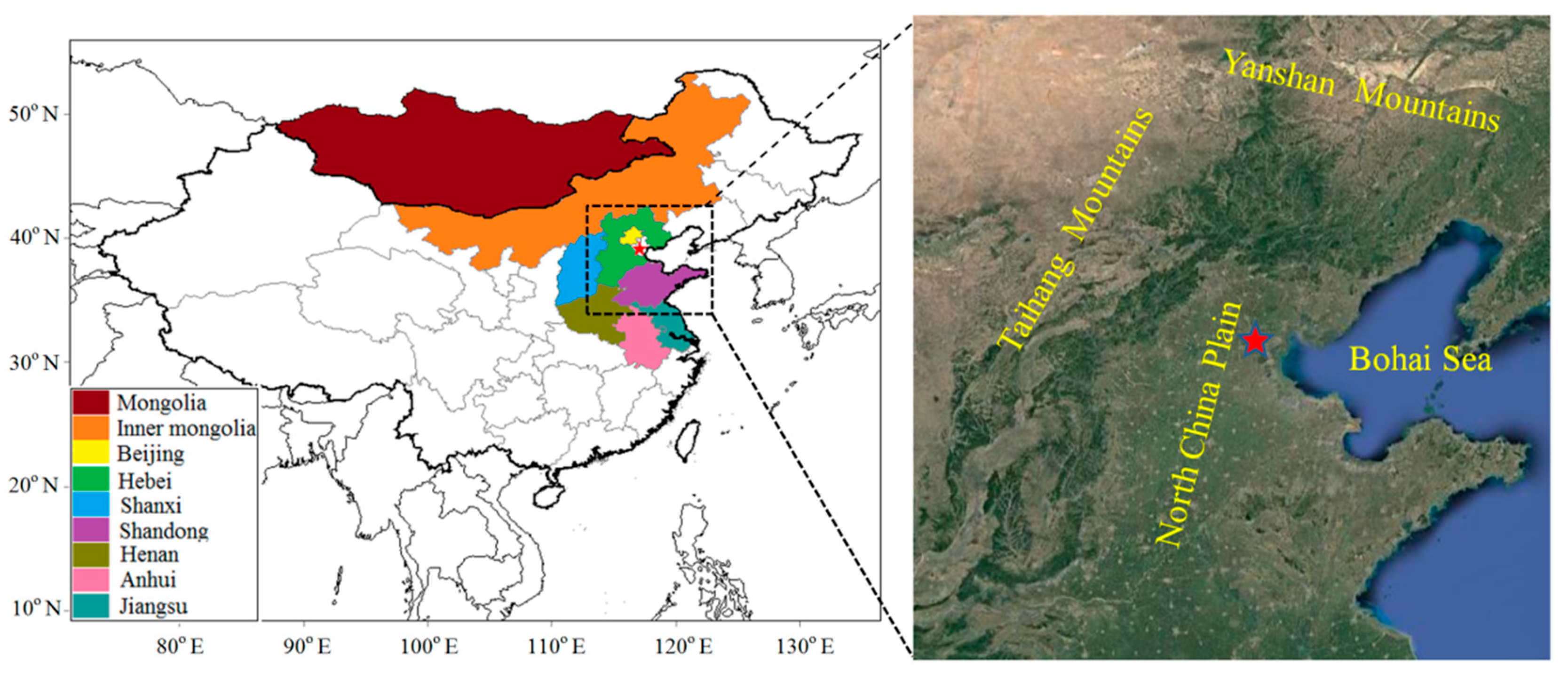
2.1. Site Location and Data

The area of interest in this study is located on the west coast of Bohai Bay (39°06′ N, 117°10′ E) (Figure 1). The land slopes downwards gradually from northwest to southeast. Tianjin is confined by Taihang Mountain to the west, the Bohai Sea to the east, Yanshan Mountain to the north, and a plain to the south. It is one of the four municipalities of China and is one of the fast-growing economic megacities in the Beijing–Tianjin–Hebei urban agglomeration. Rapid economic development has resulted in an increase in the emissions of aerosol and a concomitant increase in aerosol levels in ambient air.

The hourly average PM_2.5 mass concentration data for Tianjin from January 2009 to February 2018 used in this study were obtained from the National Urban Air Quality Real-Time Publishing Platform (http://106.37.208.233:20035/) (January 2014–February 2018) and the Tianjin atmospheric boundary layer observation station (January 2009–December 2013). The PM_2.5 data from the National Urban Air Quality Real-Time Publishing Platform, which was released by the China National Environmental Monitoring Center, represented the average PM_2.5 levels in Tianjin. The mean PM_2.5 concentration values were computed from 13 state-controlled monitoring sites in Tianjin. The PM_2.5 concentration data released by the China National Environmental Monitoring Center began in 2014. In order to analyze the long-term characteristics of PM_2.5, the monitoring data from the Tianjin atmospheric boundary layer observation station of the China Meteorological Administration from 2009 to 2013 were combined. Both datasets were obtained from oscillating microbalance measurements. An equivalence trail was carried out between them from 2014 to 2016. The results of this trail were used to correct the PM_2.5 concentration data from 2009 to 2013.

The anthropogenic emissions PM_2.5 data from 2016 were from a multiresolution emissions inventory for China (http://www.meicmodel.org/dataset-meic.html). The spatially disaggregated anthropogenic emissions inventory grids emissions were from power generation, industry, residential heating, and transportation at a resolution of 0.50° × 0.50° latitude–longitude. The hourly wind speed and direction data used to create wind roses were obtained from the Tianjin Meteorological Service. In a meteorological sense, March to May, June to August, September to November, and December to February (the following year) were defined as spring, summer, autumn, and winter, respectively.

2.2. Backward Trajectory and Cluster Analysis

The individual 3D trajectories were calculated using NOAA HYSPLIT4.9 with Global Data Assimilation System (GDAS) meteorological data, which supplies 3-h, global 1° latitude–longitude datasets of the pressure surface. Seventy-two-hour back trajectories were calculated at 6-h intervals (00:00 h, 06:00 h, 12:00 h, and 18:00 h UTC) for every day in the period of interest, for an arrival height of 200 m. At a height of 200 m, particles are well mixed under various weather conditions [32], and elevated or degraded air masses could both reach the 200-m receptor height.

To explore the impact of air mass transport on PM_2.5, backward trajectories of air parcels were clustered using the Euclidean distance method based on the TrajStat software developed by Wang et al. [33]. The Euclidean distance method is often used to define the distance between two trajectories using latitude and longitude locations as variables. The “eyeball” method (Wang et al., 2009; Wang et al., 2015) is used to determine the cluster numbers in this software. In this analysis, a cluster number of 6 was decided. The 6 clusters provided the most appropriate representation of air mass classifications according to the “eyeball” method. Trajectories with PM_2.5 > 75.00 μg/m³ were considered to be polluted trajectories, which is China’s national class II standard of PM_2.5 daily mean concentration [34].

2.3. Potential Source Contribution Function (PSCF)

Potential source regions of concentration back trajectories for PM_2.5 can be identified through a PSCF, which analyzes trajectory pathways [35,36,37] (Zeng and Hopke, 1989; Polissar et al., 1999; Begum et al., 2005). To calculate the PSCF, the whole geographic region covered by the trajectories is divided into an array of grid cells whose size is dependent on the domain of the back trajectories. The PSCF values for these grid cells are calculated by counting the trajectory segment endpoints that terminate within each cell. The number of endpoints that fall in the ijth cell are marked as n_ij. The number of endpoints in the ijth cell having the same arrival times at the sampling site corresponding to pollutant concentrations higher than an arbitrary criterion are denoted as m_ij. The PSCF value for the ijth cell is defined as

$${\mathrm{PSCF}}_{\mathrm{ij}}={\mathrm{m}}_{\mathrm{ij}}/{\mathrm{n}}_{\mathrm{ij}}$$

(1)

The PSCF value can be interpreted as a conditional probability that describes the spatial distribution of probable source locations. Cells with high PSCF values are potential source areas and should coincide with a pollutant emissions region within the domain. These cells are indicative of areas of “high potential” for contributions to receptor site pollution. However, cells with low PSCF values do not indicate low emissions, because emissions may not be transported to the receptor site.

The PSCF grids cover a domain between 20 and 70° N and 75 and 130° E, with a 0.50° × 0.50° resolution. To reduce uncertainty in cells with small n_ij values, an arbitrary weight function W (n_ij) is multiplied into the PSCF value [38,39,40,41] (Polissar et al., 2001a,b; Karaca et al., 2009; Xu et al., 2010). Equation (2) was used to obtain the weight function in this study:

$$W_{ij}=\{\begin{array}{l}1.0080<{\mathrm{n}}_{ij}\\ 0.7020<{\mathrm{n}}_{ij}\le 80\\ 0.4210<{\mathrm{n}}_{ij}\le 20\\ 0.05{\mathrm{n}}_{ij}\le 10\end{array}$$

(2)

At last, the WPSCF is expressed as

$$\mathrm{WPSCF}=W_{ij}\times \mathrm{PSCF}$$

(3)

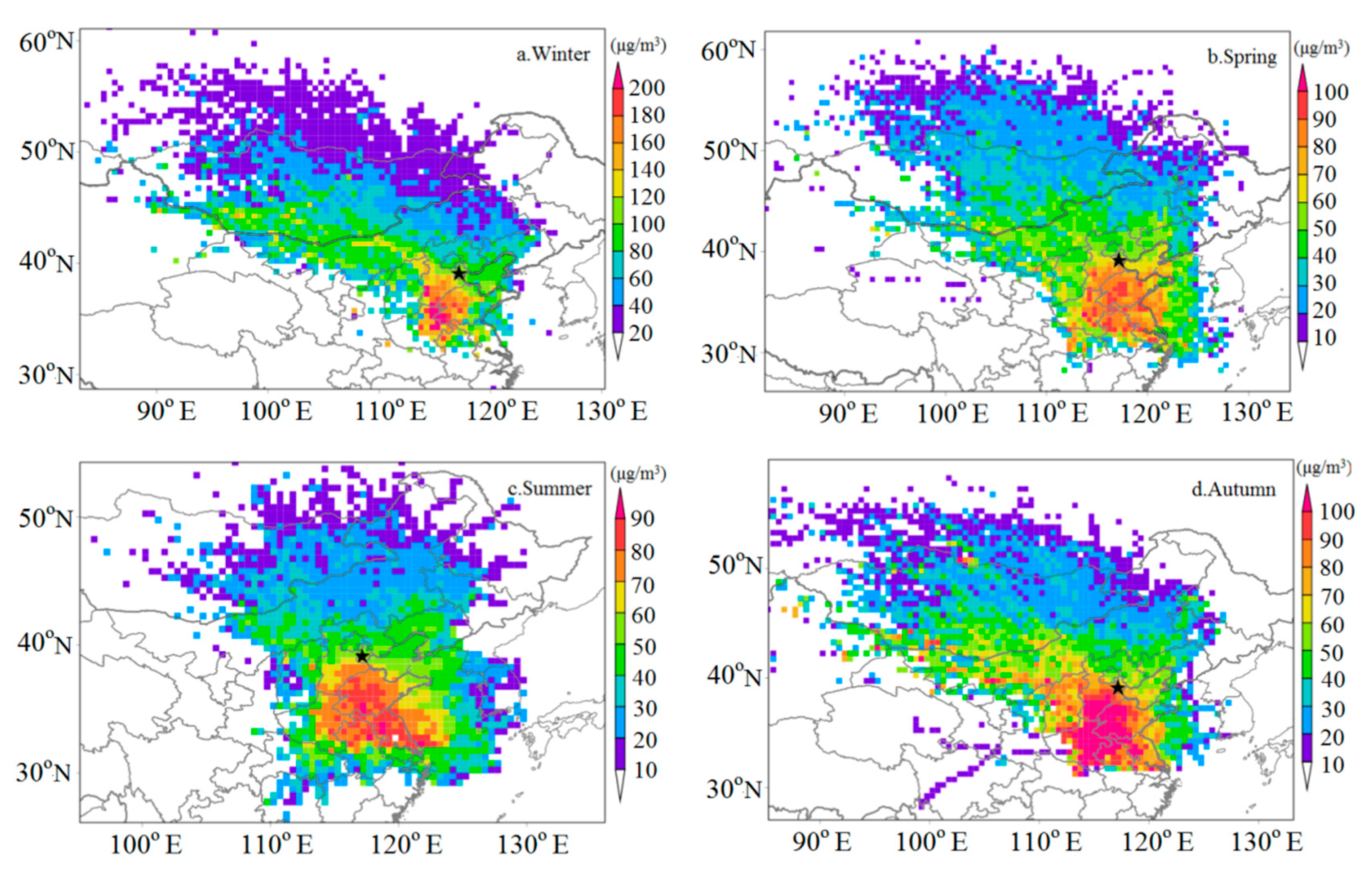
2.4. Concentration Weighted Trajectory (CWT)

A limitation of the PSCF method is that grid cells could have the same PSCF value when sample concentrations are either only slightly higher or much higher than the criterion. As a result, it cannot distinguish strong sources from moderate ones. Therefore, CWT [17,29,30] was used in this study. CWT can more easily distinguish source strength by assigning the concentration values at the receptor site to their corresponding trajectories. In the CWT method, a grid is superimposed over the domain of trajectory computations. Each grid cell is assigned a residence-time-weighted concentration from the measured sample associated with the trajectories that crossed that grid cell, as follows:

$$C_{ij}=\frac{1}{{{\displaystyle \sum }}_{l=1}^M{\tau }_{ijl}}{{\displaystyle \sum }}_{l=1}^M{c}_l{\tau }_{ijl},$$

(4)

where C_ij is the average weighted concentration in the ijth cell, l is the index of the trajectory, M is the total number of trajectories, C_l is the concentration observed on arrival of trajectory l, and τ_ijl is the time spent in the ijth cell by trajectory l. A high value for C_ij implies that air parcels traveling over the ijth cell are associated with high concentrations at the receptor.

To minimize the inaccuracy caused by the small number of polluted trajectories, arbitrary weight functions are needed to reduce uncertainty, and the empirical weight function W_ij for PSCF can also be used in the CWT method. The WCWT is defined as

$$\mathrm{WCWT}=W_{ij}\times C_{ij}.$$

(5)

3. Results and Discussions

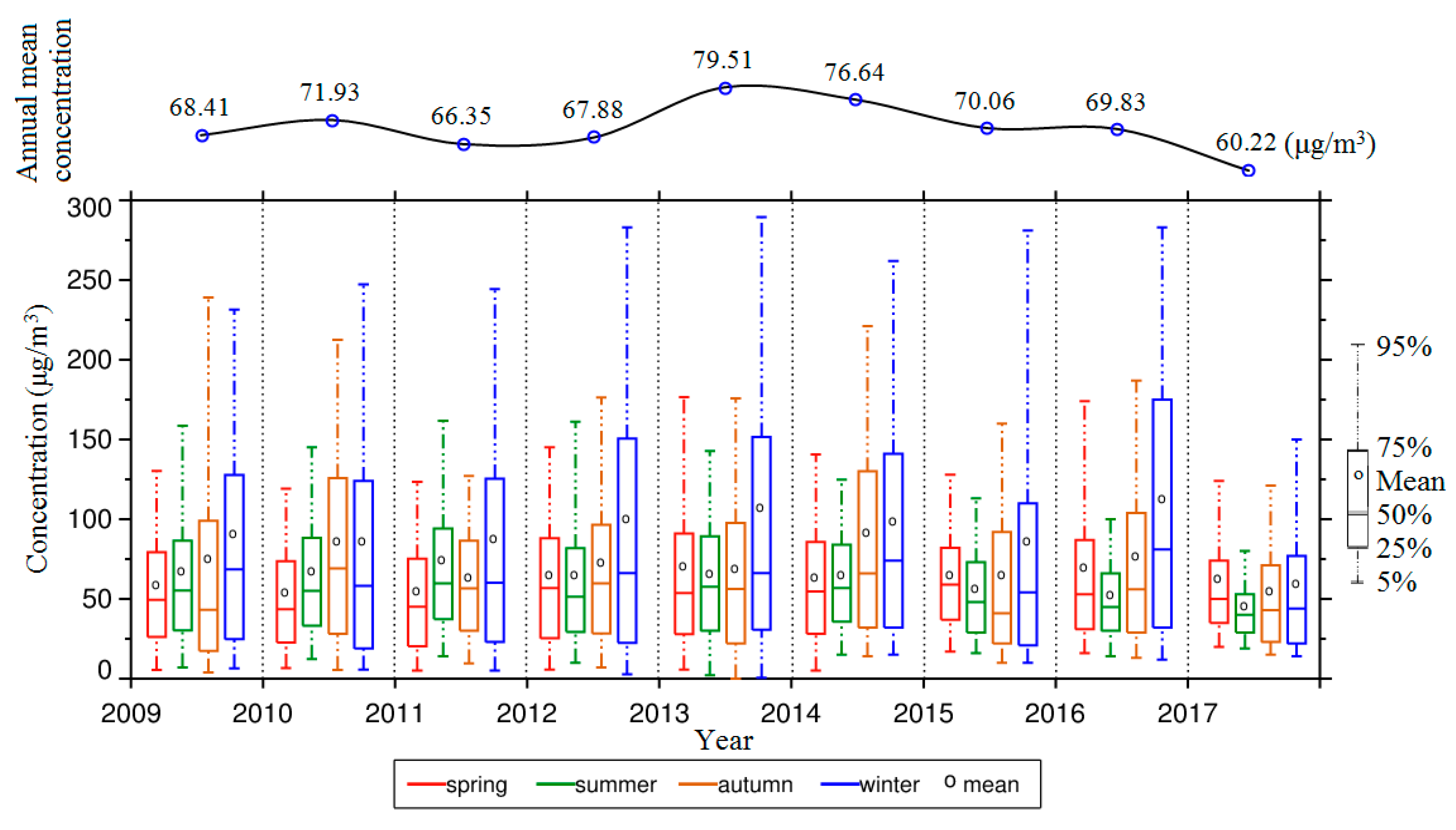
3.1. Variation in PM_2.5 Concentrations

Seasonal and annual variations of PM_2.5 concentrations from 2009 to 2018 in Tianjin are shown in Figure 2. The PM_2.5 time series shows that annual PM_2.5 levels varied between 68.41 and 67.88 μg/m³ from 2009 to 2012, reaching their maximum value (79.51 μg/m³) in 2013 and then declining steadily ever since. Throughout the whole study period, PM_2.5 levels exceeded the class II standard of the Chinese National Air Quality Standards (75.00 μg/m³) [34] and exhibited considerable seasonal variations. On average, high PM_2.5 concentrations in Tianjin always occurred in the winter, followed by autumn and spring, then summer. The mean concentrations and concentrations above the 75th percentile were higher in winter than in the other three seasons. The highest winter mean PM_2.5 concentration (109.98 μg/m³) was observed in 2016, while the lowest winter mean value of 57.20 μg/m³ was observed in 2017.

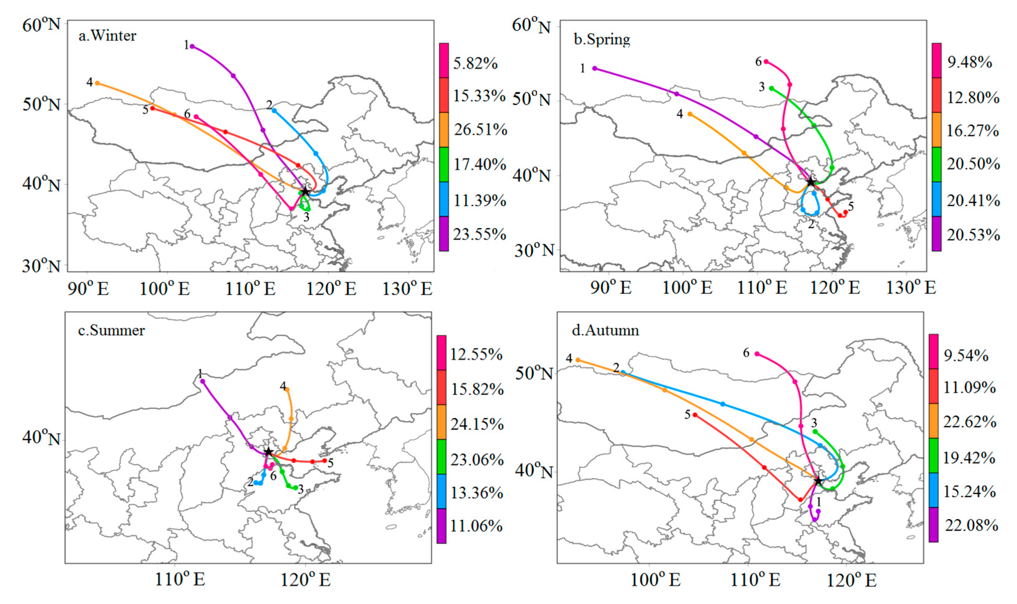
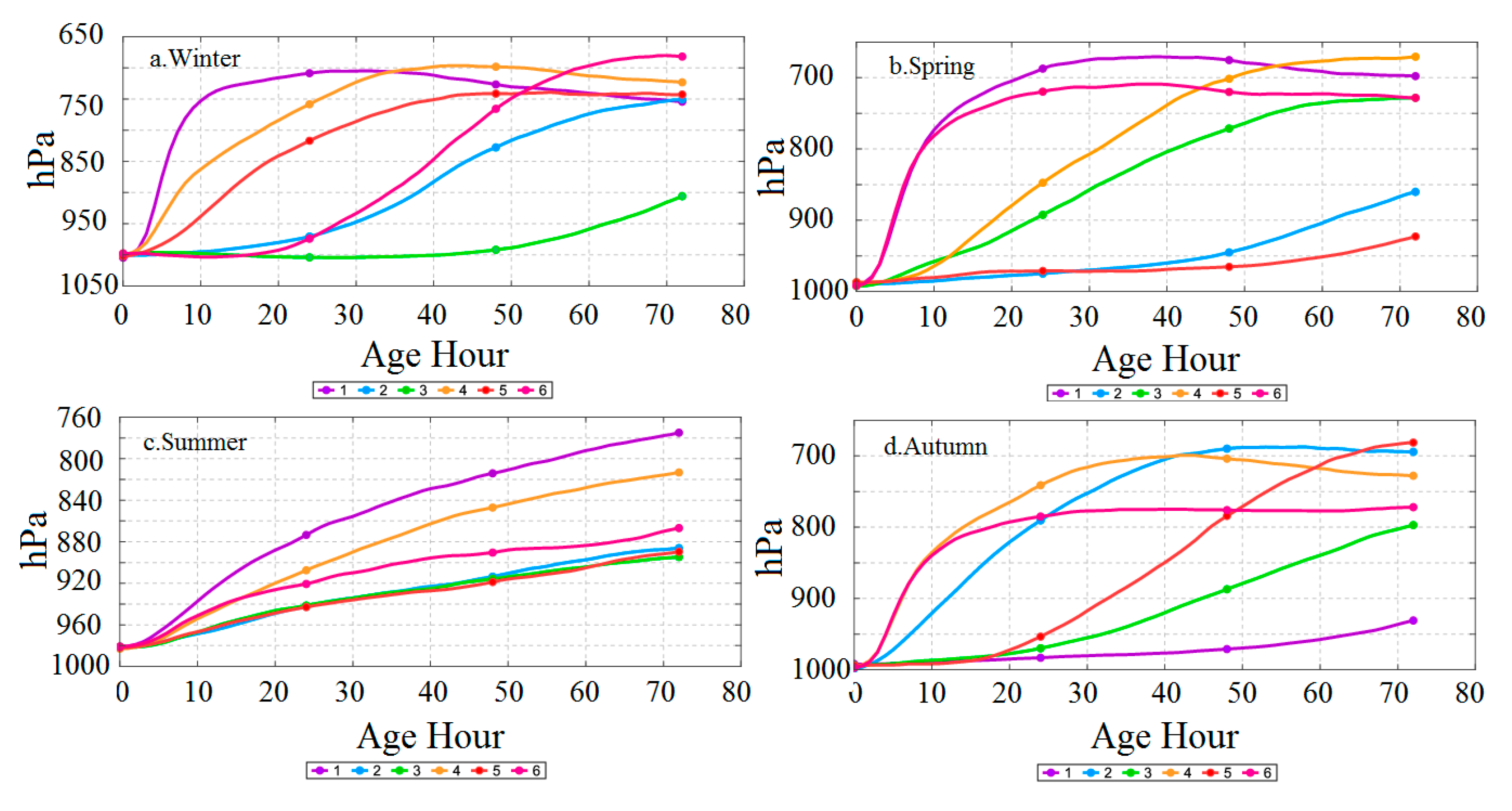
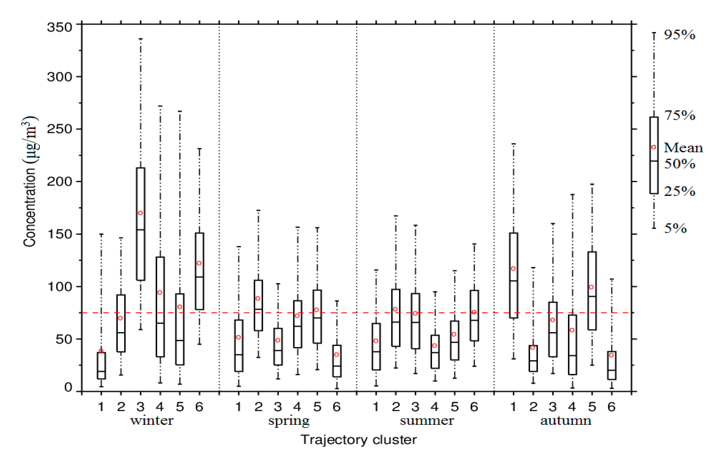
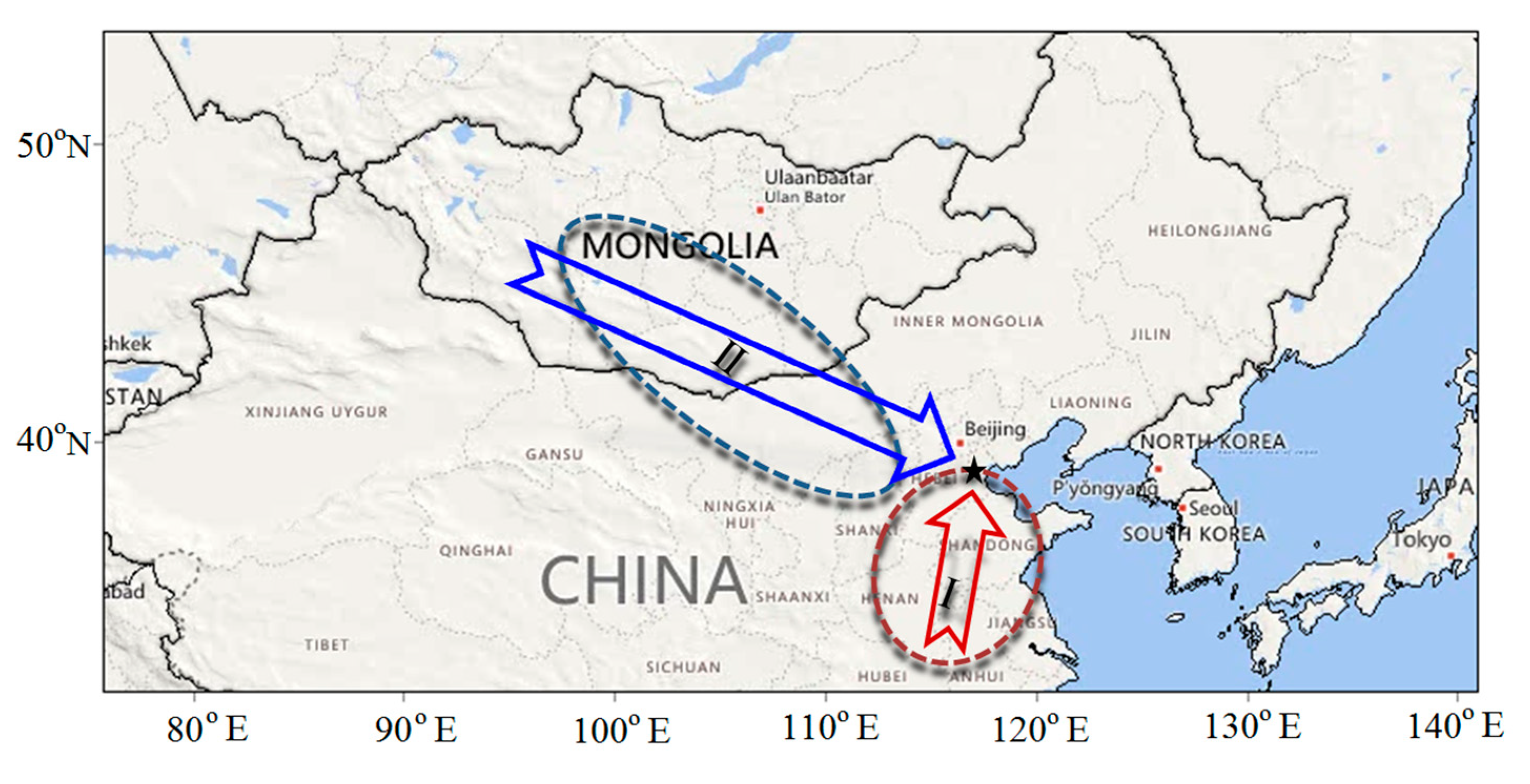
3.2. Transport Pathways

Six clusters were produced by the clustering algorithm for Tianjin from March 2009 to February 2018, and the cluster-mean back trajectories and their air pressure profiles are shown in Figure 3 and Figure 4. Distributions of PM_2.5 concentrations associated with six trajectory clusters on a seasonal basis are presented in Figure 5. The velocity of air mass movement could be judged according to the length of the trajectory. Long trajectories corresponded to fast-moving air masses, while short trajectories corresponded to slow-moving air masses. According to the mean PM_2.5 mass concentration of Tianjin corresponding to each cluster, the cluster-mean backward trajectories were divided into clean pathways and pollution pathways. A cluster-mean backward trajectory corresponding to a PM_2.5 concentration in Tianjin > 75.00 μg/m³ was defined as a pollution pathway. On the contrary, a cluster-mean backward trajectory corresponding to a PM_2.5 concentration in Tianjin < 75.00 μg/m³ was defined as a clean pathway. A cluster-mean back trajectory was also defined as a pollution pathway if the amount of pollution trajectories in this cluster accounted for more than one-sixth of the total number of pollution trajectories.

In winter, it was found that four out of the six cluster trajectories, represented by clusters 3, 4, 5, and 6, were pollution pathways. Among these four major pathways, the one shown as cluster 3 accounted for 17.40% and was the most polluted. More than 85% of its sample concentrations exceeded the daily class II standard of PM_2.5, and the mean concentration (168.00 μg/m³) was far above the daily standard concentration (Figure 5). Cluster 3 originated from Hebei, went through Shandong, and reached Tianjin. This was a regional transport pathway within a boundary layer (Figure 4a). Its short length suggested low wind velocity. Low wind velocity and relatively low boundary layer heights in winter may exacerbate air pollution, contributing to a severe haze episode. The second most polluted pathway was cluster 6, which meant the concentration was 120.00 μg/m³. More than 75% of the sample concentrations exceeded daily class II standard concentrations (Figure 5). The air masses associated with cluster 6 were from Central Mongolia, moved southeasterly over the Inner Mongolian Plateau and into Hebei, and finally turned northeast to Tianjin. The air masses of cluster 6 from the southwest were transported in the boundary layer and slowed down in the first 24 h. Cluster 4, which meant the concentration was 92.00 μg/m³, was the prevalent trajectory pathway in winter (26.51%). The air masses associated with both clusters 4 and 5 initially traveled southeasterly over desert and semidesert regions of Mongolia and the Hunshandake sand lands of Inner Mongolia. Cluster 4 air masses then went southeasterly though Hebei and Beijing to Tianjin. Cluster 5 finally turned northwest though Hebei to Tianjin. Clusters 4, 5, and 6 all passed though Mongolia and Inner Mongolia: A study by Zhao et al. [42] showed that long-range transport from Inner Mongolia also had an adverse effect on PM_2.5 in Shanghai. Clusters 1 and 2 were clean pathways for Tianjin in winter. The air masses associated with clusters 1 and 2 originated from Lake Baikal and Outer Mongolia. Cluster 1 air masses moved rapidly and traveled at heights greater than 750 hPa for the 10 h before arrival in Tianjin. Cluster 2 represented a relatively slow-moving air mass, particularly in the 24 h preceding its arrival in Tianjin. It reached Tianjin through the Bay of Bohai and was considered to be a relatively clean trajectory. It can be seen from

Table 1. Trajectory percentage and mean PM_2.5 concentrations based on all trajectories and pollution trajectories.

Season	Cluster	Number of All Trajectories per Cluster	Percentage of Pollution Trajectories in Each Cluster (%)	Percentage of Pollution Trajectories in Total Pollution Trajectories Per Season (%)	Mean Concentration and Standard Deviation of Pollution Trajectories (μg/m3)
Winter	1	620	12.10	6.40	147 ± 74
	2	323	34.40	9.50	116 ± 43
	3	490	89.60	37.70	182 ± 82
	4	690	42.20	25.00	167 ± 91
	5	393	31.30	10.60	176 ± 109
	6	161	77.60	10.70	140 ± 53
Spring	1	553	21.90	14.40	117 ± 44
	2	574	55.40	37.90	114 ± 37
	3	588	14.30	10.00	106 ± 33
	4	454	33.50	18.10	116 ± 48
	5	325	44.00	17.00	112 ± 33
	6	250	8.40	2.50	107 ± 46
Summer	1	324	18.20	6.90	108 ± 27
	2	395	42.80	19.70	117 ± 38
	3	717	40.00	33.40	114 ± 35
	4	714	10.90	9.10	99 ± 21
	5	499	19.40	11.30	107 ± 40
	6	388	43.30	19.60	108 ± 30
Autumn	1	588	71.40	42.40	142 ± 57
	2	377	9.30	3.50	144 ± 73
	3	538	32.00	17.40	119 ± 40
	4	593	24.30	14.50	144 ± 73
	5	320	60.10	19.70	129 ± 42
	6	226	10.60	2.40	117 ± 37

that the highest percentage of polluted trajectories (37.70%) and the highest PM_2.5 loading (182.00 μg/m³) were observed in cluster 3, followed by clusters 4 and 6. In addition, 89.60% of total trajectories in cluster 3 were polluted trajectories, and 25.00% and 10.70% of total polluted trajectories were from the cluster 4 and cluster 6 trajectories, respectively: 77.60% of the trajectories in cluster 6 were polluted.

In spring, the pollution pathways associated with trajectory clusters 2, 4, and 5 accounted for 20.41%, 16.27%, and 12.80% (Figure 3). Cluster 2 was the major pollution pathway, followed by clusters 4 and 5. The mean concentrations of clusters 2, 4, and 5 were 87.00 μg/m³, 70.00 μg/m³, and 76.00 μg/m³ (Figure 5). Clusters 2 and 5 were both short pathways and were transported into the boundary layer. Cluster 2 air masses were from Northern Shandong and traveled southerly, finally going northerly through Shandong to Tianjin. Cluster 5 air masses originated from the Bohai Sea and then traveled northwesterly through Shandong to Tianjin. Thus, the pathways through Shandong were noticeable for Tianjin in the spring. Cluster 4 was from Central Mongolia, moving southeasterly over Inner Mongolia, Shanxi, and Hebei and finally turning northeasterly to Tianjin. The air masses of cluster 4 were transported below 925 hPa and slowed down in the first 20 h before reaching Tianjin (Figure 4b). The one shown as cluster 2 had the largest percentage (37.90%) of polluted trajectories and a higher mean loading (114.00 μg/m³) (Table 1). More than half of the trajectories in cluster 2 were pollution trajectories. Although the mean concentration of cluster 4 in spring did not exceed the class II standard concentration, the pollution trajectories in cluster 4 accounted for 18.10% of the total pollution trajectories. Cluster 5 contributed 17.00% of the total pollution trajectories.

In summer, the higher levels of PM_2.5 concentration in Tianjin coincided with trajectories grouped in clusters 2, 3, and 6, which were all southerly short pathways and accounted for 48.97% of the total number of trajectories (Figure 3). The mean concentrations of clusters 2, 3, and 6 were 77.00 μg/m³, 72.00 μg/m³, and 74.00 μg/m³. Cluster 2 and cluster 3 originated from northwestern and eastern Shandong, respectively, and traveled north in the 24 h preceding their arrival in Tianjin. Cluster 6 originated from Hebei and traveled south to Shandong and then north to Tianjin. The transport heights of pollution pathways were all less than 850 hPa (Figure 4c). Cluster 3 had the largest percentage (33.40%) of polluted trajectories, and the pollution pathways accounted for 40.00% of all pathways for cluster 3 (Table 1).

In autumn, clusters 1, 3, and 5 were the pollution pathways, the mean concentrations of which were 115.00 μg/m³, 66.00 μg/m³, and 98.00 μg/m³. Cluster 1 originated from Shandong and went northerly to Tianjin, the transport height of which was less than 925 hPa (Figure 4d). Cluster 3 originated from Inner Mongolia and passed over the Bohai Sea and Shandong before reaching Tianjin. This was the only pollution pathway through the sea. However, in the 24 h preceding its arrival in Tianjin, the air masses of cluster 3 arrived in Shandong and moved slowly, the heights of which were below 925 hPa. Cluster 5 in autumn, similarly to cluster 6 in winter, was from Central Mongolia, moved southeasterly over the Inner Mongolian Plateau and into Hebei, and finally turned northeasterly to Tianjin. The air masses of cluster 5 from the southwest direction were transported below 925 hPa and slowed down in the 24 h preceding their arrival in Tianjin. The highest probability (71.40%) of pollution trajectories occurred in cluster 1, which contributed 42.00% of polluted trajectories (Table 1). The mean loading of polluted trajectories in cluster 1 was 142.00 μg/m³, 60.10% of the trajectories in cluster 5 were pollution trajectories, and 19.70% and 17.40% of pollution trajectories came from cluster 5 and cluster 3, respectively.

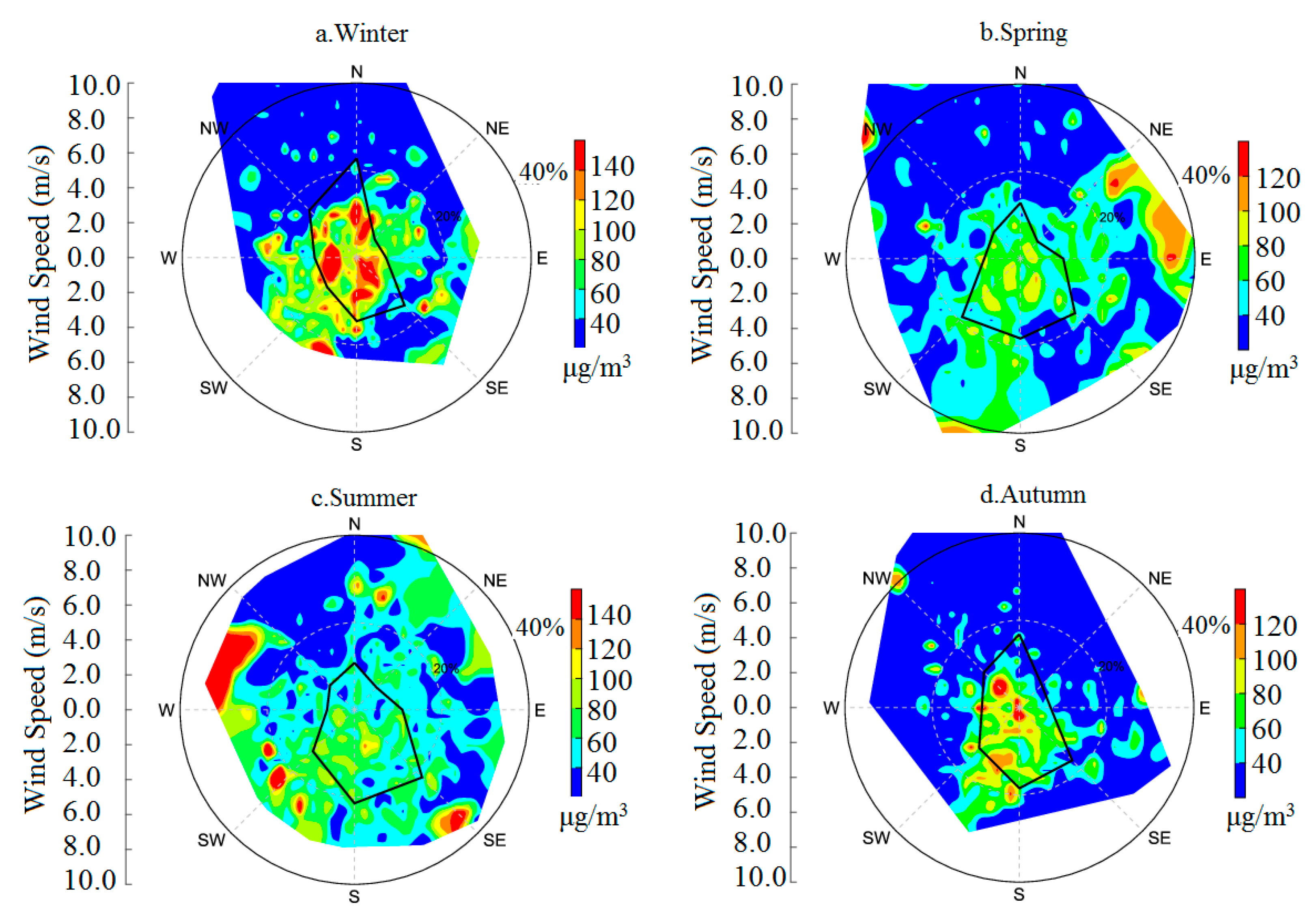
3.3. Wind Dependence of PM_2.5 Loadings

The seasonal wind roses with PM_2.5 loadings on the west coast of Bohai Bay using hourly data for 2009–2018 are shown in Figure 6. The prevailing winds for winter were between the north and the northwest. Most of winds were abundant, with the south and southeast as the prevailing wind directions in summer. The variation in wind direction in different seasons is because this area is located in a monsoon zone, with prevailing winds from northern directions during winter and from southern directions during summer. Winds from the northwest and north originate from or pass over economically underdeveloped regions in China with relatively lower PM_2.5 emissions intensities.

PM_2.5 loadings showed pronounced dependence on the wind, especially in the heavily polluted autumn and winter. As shown in Figure 6a, high PM_2.5 concentrations were mainly concentrated in low wind speed (0–2 m/s) areas and were associated with winds from the south and west. Southern winds and western winds were normally from the Shanxi, Shandong, and Hebei provinces. Regardless of the wind directions, PM_2.5 loadings were below 40.00 μg/m³ when the wind speeds were greater than 6 m/s. Most of the high PM_2.5 loadings in autumn were associated with winds from the south and southwest, and wind speeds were all in the range of 0–5 m/s. The situation in spring and summer showed a similar but less pronounced directional dependence compared to winter and autumn. High PM_2.5 loadings were observed with northeasterly to easterly flows in spring (Figure 6b) and northwesterly to westerly flows in summer (Figure 6c). Overall, the southwesterly winds had an adverse effect on PM_2.5 loadings in different seasons for Tianjin. In contrast, wind from the northwest to north sectors normally showed mean PM_2.5 loadings lower than 40.00 μg/m³.

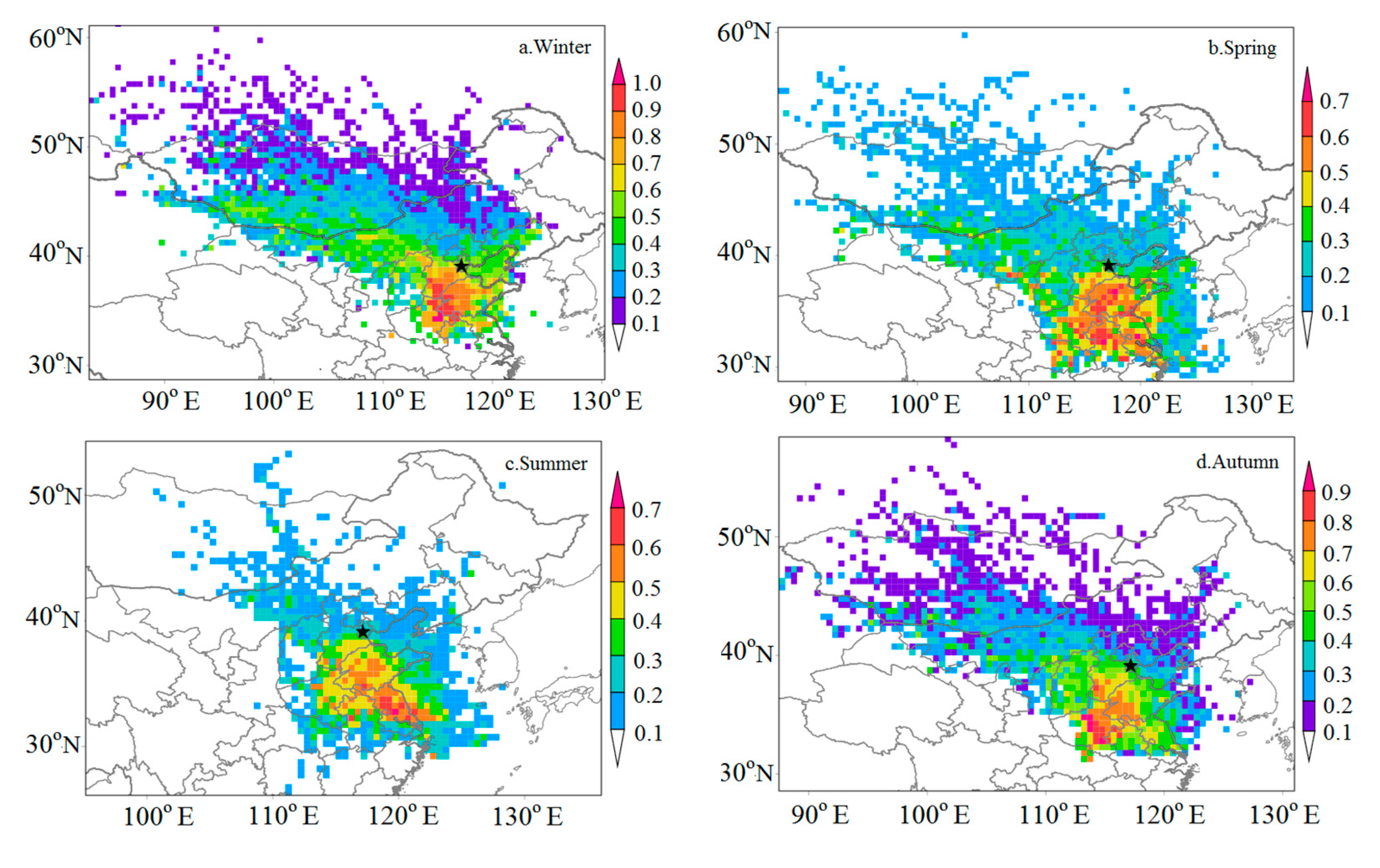
3.4. Potential Source Regions

The PSCF maps covering the study period that are shown in Figure 7 were plotted in order to identify the probable locations of potential source regions contributing to PM_2.5 levels in Tianjin on the west coast of Bohai Bay. In general, the main source areas were all in the south of Tianjin. The potential source areas for winter were larger than for other seasons. In winter, the major source areas of PM_2.5, with WPSCF values of 0.80–1.00, were in the junction of Hebei, Henan, and Shandong. Northern Shandong, southern Hebei, northeastern Henan, northern Shanxi, central Inner Mongolia, and northern Mongolia were also potential source areas of PM_2.5, with WPSCF values of 0.50–0.80. This was mainly because these areas, except for Inner Mongolia and Mongolia, are economically developed industrial areas, and pathways of air masses ended at Tianjin. The Gobi Desert in central Inner Mongolia and northern Mongolia was a natural source of PM_2.5. In autumn, the major potential sources were located in eastern Henan, northwestern Shandong, and northern Hebei (Figure 7d). North central Hebei, central Shandong, Shanxi, northern Jiangsu, and northern Anhui were the second potential source areas. The domains of major sources in winter and autumn were all concentrated in the southwest of Tianjin, which revealed that transport from the southwest was more important for heavy PM_2.5 pollution in winter and autumn. The potential source regions determined from the PSCF analysis coincided with the results from the wind dependence of PM_2.5 loadings. However, the major potential source areas varied seasonally. In spring, major sources of PM_2.5, with WPSCF values of 0.50–0.70, were in Shandong, eastern Henan, and northern Anhui and Jiangsu, and for summer were in northern Jiangsu and western Shandong.

Since the PSCF method can only reflect the contribution rate of the potential source regions, that is, the proportion of pollution trajectories in each grid, it cannot reflect the pollution degree of the potential source regions. In order to study the contribution of pollutants in potential source regions, the CWT method was used to reflect the pollution degree of different trajectories. The results for PM_2.5 loadings identified through the CWT method in Figure 8 were somewhat different from the results analyzed through the PSCF method. WCWT values do not represent the regions’ actual contributions. Instead, they demonstrate the relative importance of the source regions [31]. In winter, the highest WCWT values covering the map were distributed in southern Hebei, western Shandong, and northeastern Anhui. Those areas were the main contribution sources associated with the highest PM_2.5 loadings (exceeding 140.00 μg/m³), and the border between Anhui and Shandong was even higher than 200.00 μg/m³. This demonstrated that contributions of transportation and source regions from southern Tianjin were significant. As shown in Figure 8a, there were also secondary source areas in winter, namely central Inner Mongolia and southern Mongolia. These areas are normally characterized by land forms of sand and the Gobi Desert. Besides the impact of local and regional potential sources, long-range transport also played some role in PM_2.5 loadings in winter. This depended on both the prevailing northwest wind in Tianjin and potential source areas to the northwest, contributing to the long-rang transport of PM_2.5. In spring and summer, the maximum WCWT was much smaller than in winter. The significant potential source regions in spring were identified south of Tianjin, including southern Hebei, Shandong, eastern Henan, northern Anhui, and Jiangsu. In addition to the above areas, a small part of the Yellow Sea was also included in the summer (adjacent to Jiangsu province). In autumn, the highest WCWT values (exceeding 100.00 μg/m³) were mainly located in southern Hebei, western Shandong, eastern Henan, the northwest corner of Anhui, and parts of Jiangsu. The second potential source areas were Shanxi, central Shandong, and northern Jiangsu.

The PSCF and CWT analyses gave similar potential source locations, but the contributions of these locations were different. The major potential source areas derived from the CWT method were larger than those of the PSCF method, especially in autumn and summer. Regional sources might play a more pronounced role in the distribution of PM_2.5 in Tianjin. The most possible major source regions of PM_2.5 were located within about 800 km south of Tianjin, and no significant long-range transport processes contributed to PM_2.5 loadings in Tianjin except for in winter and autumn.

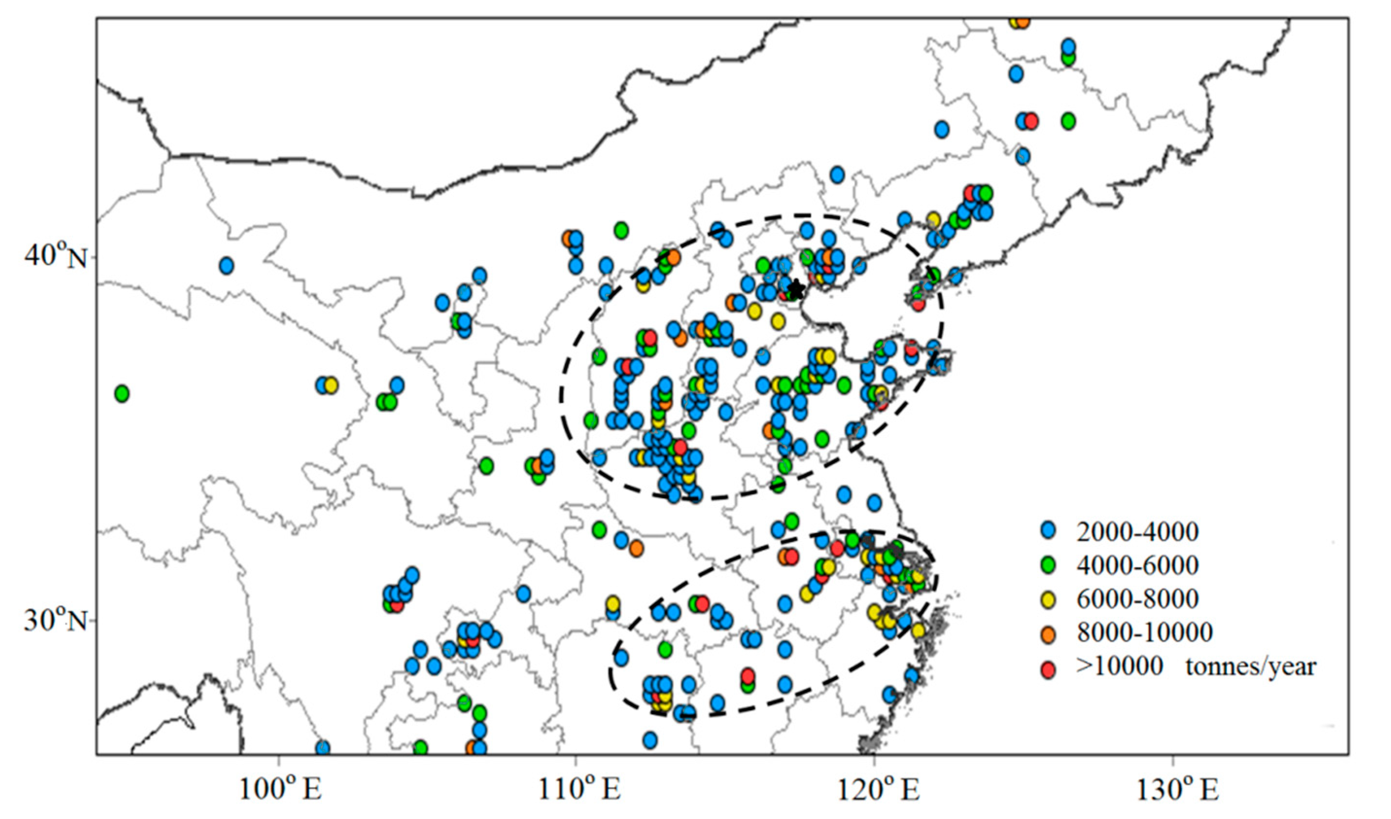
3.5. Comparison to Anthropogenic Emissions Inventory

The spatially disaggregated Chinese anthropogenic emissions inventory for PM_2.5 in 2016 is shown in Figure 9. Most of the PM_2.5 emission sources were concentrated in the Beijing–Tianjin–Hebei region and its surrounding areas, including Beijing, Tianjin, Hebei, Shandong, Shanxi, and Henan (see Figure 9). Beijing–Tianjin–Hebei and its surrounding areas are urbanized and industrialized regions with high anthropogenic PM_2.5 emissions. In North China, there are densely populated regions, numerous metallurgical works, and coal-related industries. Other regions with high concentrations of emissions sources are the Yangtze River Delta, which includes Shanghai, Jiangsu, and Zhejiang, and some parts of the southwest.

According to the above research, the potential sources of Tianjin were mainly composed of two regions (Figure 10). The major sources were the south of Tianjin, including southern Hebei, western Shandong, eastern Henan, northern Anhui, and northern Jiangsu. The secondary sources, which were northwesterly sources, encompassed central Inner Mongolia and southern Mongolia. The potential source regions determined from the PSCF and CWT analyses coincided with the emissions of PM_2.5 in North China and the results from the wind dependence of PM_2.5 loadings. Based on the above results, we preliminarily considered that the major source areas were anthropogenic sources and the secondary source areas were natural sources. This conclusion was consistent with the fact that dust aerosols are transported to Beijing from northwestern regions in spring [43,44], and anthropogenic aerosols are transported from the south [45,46]. The pathways were classified into two broad categories according to the distribution of directions of pollution clusters in Tianjin. Thus, the southerly pathway and northwesterly pathway were two major transport channels contributing to high PM_2.5 concentrations in Tianjin. The southerly transport pathway from major sources, namely the regional transport pathway, played an important role in PM_2.5 concentrations in all seasons in Tianjin. It had the greatest impact on PM_2.5 levels registered during winter, followed by autumn, and had the least impact in summer. Air masses originating from major sources probably were transported within the boundary layer and moved slowly to Tianjin. The northwesterly transport pathway from secondary sources, namely the long-range transport pathway, affected PM_2.5 concentrations in the winter, autumn, and spring. This conclusion was different from that reached by Liang et al. [20] in Beijing, where a long-rang transport from the northwest was identified as the prevailing PM_2.5 pollution transport in spring and in summer. The influence of the northwesterly pathway on PM_2.5 concentrations in Tianjin was also less than that of the southerly pathway.

4. Conclusions

Transport pathways and potential source regions of PM_2.5 on the west coast of Bohai Bay were identified through cluster trajectory, PSCF, and CWT methods based on 2009–2018 data. The annual PM_2.5 levels varied between 68.41 and 67.88 μg/m³ from 2009 to 2012, reaching their maximum value (79.51 μg/m³) in 2013 and then declining steadily ever since. High PM_2.5 concentrations always occurred in the winter, followed by autumn and spring.

Two transport pathways of high PM_2.5 concentrations in the west coast of Bohai Bay (in the broad sense) were identified, namely a southerly pathway and a northwesterly pathway. The southerly pathway represented the major transport pathway of PM_2.5 for all seasons. It had the greatest impact in winter, followed by autumn. The air masses associated with the southerly pathway were transported within the boundary layer (below 925 hPa) and moved slowly to Tianjin. The southerly transport pathway passed over the Shandong and Hebei provinces before reaching Tianjin. The northwesterly pathway belonging to long-range transport mainly affected PM_2.5 concentrations in winter and moved faster. The northwesterly pathways passed over desert and semidesert regions in Outer Mongolia, the sand lands of Inner Mongolia, and Hebei.

The potential source regions contributing to high PM_2.5 loadings on the west coast of Bohai Bay could be grouped into two broad categories, the “southerly source regions” (southern Hebei, western Shandong, eastern Henan, northern Anhui, and northern Jiangsu) and the “northwesterly source regions” (central Inner Mongolia and southern Mongolia). The “southerly source regions” were decided upon after a comparison to the Chinese spatially disaggregated anthropogenic emissions inventory and were identified as anthropogenic source regions, while the “northwesterly source regions” were regarded as natural source regions. Moreover, the major transport pathway passed over anthropogenic source regions, while the secondary transport pathway passed though natural source regions. The impacts of anthropogenic source regions on PM_2.5 loadings on the west coast of Bohai Bay were much greater than those of natural source regions. However, additional studies on the secondary reaction of PM_2.5 on the west coast of Bohai Bay are warranted to elucidate the variability in potential source regions of PM_2.5.

It can be seen from the above results that adjacent source regions had a relatively great impact on PM_2.5 concentrations on the west coast of Bohai Bay. Therefore, the meteorological characteristics of each pollution pathway, such as temperature, and the specific contribution of the adjacent source regions need to be studied further in detail.

References

1. Chan, C.; Yao, X. Air pollution in mega cities in China. Atmos. Environ. 2008, 42, 1–42. [Google Scholar] [CrossRef]
2. Shao, M.; Tang, X.; Zhang, Y.; Li, W. City clusters in China: Air and surface water pollution. Front. Ecol. Environ. 2006, 4, 353–361. [Google Scholar] [CrossRef]
3. Zhao, P.; Zhang, X. Long-term visibility trends and characteristics in the region of Beijing, Tianjin, and Hebei, China. Atmos. Res. 2011, 101, 711–718. [Google Scholar] [CrossRef]
4. Fang, M.; Chan, C.K.; Yao, X. Managing air quality in a rapidly developing nation: China. Atmos. Environ. 2009, 43, 79–86. [Google Scholar] [CrossRef]
5. Zhang, M.; Song, Y.; Cai, X. A health-based assessment of particulate air pollution in urban areas of Beijing in 2000–2004. Sci. Total Environ. 2007, 376, 100–108. [Google Scholar] [CrossRef] [PubMed]
6. Alolayan, M.A.; Brown, K.W.; Evans, J.S.; Bouhamra, W.S.; Koutrakis, P. Source apportionment of fine particles in kuwait city. Sci. Total Environ. 2013, 448, 14–25. [Google Scholar] [CrossRef] [PubMed]
7. Hellack, B.; Quass, U.; Beuck, H.; Wick, G.; Kuttler, W.; Schins, R.P.; Kuhlbusch, T.A. Elemental composition and radical formation potency of PM10 at an urban background station in Germany in relation to origin of air masses. Atmos. Environ. 2015, 105, 1–6. [Google Scholar] [CrossRef]
8. Makra, L.; Ionel, I.; Csépe, Z.; Matyasovszky, I.; Lontis, N.; Popescu, F.; Sümeghy, Z. The effect of different transport modes on urban PM10 levels in two European cities. Sci. Total Environ. 2013, 458, 36–46. [Google Scholar] [CrossRef]
9. Kong, X.; He, W.; Qin, N.; He, Q.; Yang, B.; Ouyang, H.; Wang, Q.; Xu, F. Comparison of transport pathways and potential sources of PM10 in two cities around a large Chinese lake using the modified trajectory analysis. Atmos. Res. 2013, 122, 284–297. [Google Scholar] [CrossRef]
10. Zhang, R.; Jing, J.; Tao, J.; Hsu, S.C. Chemical characterization and source apportionment of PM2.5 in Beijing: Seasonal perspective. Atmos. Chem. Phys. 2014, 13, 7053–7074. [Google Scholar] [CrossRef]
11. Lai, L.W. Fine particulate matter events associated with synoptic weather patterns, long-range transport paths and mixing height in the Taipei basin, Taiwan. Atmos. Environ. 2015, 113, 50–62. [Google Scholar] [CrossRef]
12. Lv, B.; Zhang, B.; Bai, Y. A systematic analysis of PM2.5 in Beijing and its sources from 2000 to 2012. Atmos. Environ. 2016, 124, 98–108. [Google Scholar] [CrossRef]
13. Fuelberg, H.E.; Kiley, C.M.; Hannan, J.R.; Westberg, D.J.; Avery, M.A.; Newell, R.E. Meteorological conditions and transport pathways during the transport and chemical evolution over the pacific (trace-p) experiment. J. Geophys. Res. Atmos. 2003, 108, 8782. [Google Scholar] [CrossRef]
14. Reid, J.S.; Lagrosas, N.D.; Jonsson, H.H.; Reid, E.A.; Atwood, S.A.; Boyd, T.J.; Ghate, V.P.; Xian, P.; Posselt, D.J.; Simpas, J.B.; et al. Aerosol meteorology of Maritime Continent for the 2012 7SEAS southwest monsoon intensive study–Part 2: Philippine receptor observations of fine-scale aerosol behavior. Atmos. Chem. Phys. 2016, 16, 14057–14078. [Google Scholar] [CrossRef]
15. He, K.; Huo, H.; Zhang, Q. Urban air pollution in China: Current status, characteristics, and progress. Annu. Rev. Energy Environ. 2011, 27, 397–431. [Google Scholar] [CrossRef]
16. Wang, G.C.; Wang, J.; Xin, Y.J.; Chen, L. Transportation pathways and potential source areas of PM10 and NO2 in Tianjin. China. Environ. Sci 2014, 34, 3009–3016. (In Chinese) [Google Scholar]
17. Wang, Y.Q.; Zhang, X.Y.; Arimoto, R. The contribution from distant dust sources to the atmospheric particulate matter loadings at XiAn, China during spring. Sci. Total Environ. 2006, 368, 875–883. [Google Scholar] [CrossRef] [PubMed]
18. Xin, Y.J.; Wang, G.C.; Chen, L. Identification of long-range transport pathways and potential sources of PM10 in Tibetan Plateau uplift area: Case study of Xining, China in 2014. Aerosol Air Qual. Res. 2016, 16, 1044–1054. [Google Scholar] [CrossRef]
19. Zhu, L.; Huang, X.; Shi, H.; Cai, X.; Song, Y. Transport pathways and potential sources of PM10 in Beijing. Atmos. Environ. 2011, 45, 594–604. [Google Scholar] [CrossRef]
20. Liang, D.; Wang, Y.Q.; Ma, C.; Wang, Y.J. Variability in transport pathways and source areas of PM10 in Beijing during 2009–2012. Aerosol Air Qual. Res. 2016, 16, 3130–3141. [Google Scholar] [CrossRef]
21. Wang, L.; Liu, Z.; Sun, Y.; Ji, D.; Wang, Y. Long-range transport and regional sources of PM2.5 in Beijing based on long-term observations from 2005 to 2010. Atmos. Res. 2015, 157, 37–48. [Google Scholar] [CrossRef]
22. Ashbaugh, L. A statistical trajectory technique for determining air pollution source regions. J. Air Pollut. Control Assoc. 1983, 33, 1096–1098. [Google Scholar] [CrossRef]
23. Sirois, A.; Bottenheim, J.W. Use of backward trajectories to interpret the 5-year record of PAN and O3 ambient air concentrations at Kejimkujik National Park, Nova Scotia. J. Geophys. Res. Atmos. 1995, 100, 2867–2881. [Google Scholar] [CrossRef]
24. Park, S.S.; Lee, K.H.; Kim, Y.J.; Kim, T.Y.; Cho, S.Y.; Kim, S.J. High time-resolution measurements of carbonaceous species in PM2.5 at an urban site of Korea. Atmos. Res. 2008, 89, 48–61. [Google Scholar] [CrossRef]
25. Moody, J.L.; Galloway, J.N. Quantifying the relationship between atmospheric transport and the chemical composition of precipitation on Bermuda. Tellus B 1988, 40, 463–479. [Google Scholar] [CrossRef] [Green Version]
26. Harris, J.M.; Kahl, J.D. A descriptive atmospheric transport climatology for the Mauna Loa Observatory, using clustered trajectories. J. Geophys. Res. Atmos. 1990, 95, 13651–13667. [Google Scholar] [CrossRef]
27. Dorling, S.R.; Davies, T.D.; Pierce, C.E. Cluster analysis: A technique for estimating the synoptic meteorological controls on air and precipitation chemistry-method and applications. Atmos. Environ. 1992, 26, 2575–2581. [Google Scholar] [CrossRef]
28. Vasconcelos, L.A.D.P.; Kahl, J.D.W.; Liu, D.; Macias, E.S.; White, W.H. Spatial resolution of a transport inversion technique. J. Geophys. Res. Atmos. 1996, 101, 19337–19342. [Google Scholar] [CrossRef]
29. Seibert, P.; Kromp-Kolb, H.; Baltensperger, U.; Jost, D.T.; Schwikowski, M.; Kasper, A.; Puxbaum, H. Trajectory analysis of aerosol measurements at high alpine sites. In Transport and Transformation of Pollutants in the Troposphere; Borrel, P.M., Borrel, P., Cvitas, T., Seiler, W., Eds.; Academic Publishing: Den Haag, The Netherlands, 1994; pp. 689–693. [Google Scholar]
30. Stohl, A. Trajectory statistics-a new method to establish source-receptor relationships of air pollutants and its application to the transport of particulate sulfate in Europe. Atmos. Environ. 1996, 30, 579–587. [Google Scholar] [CrossRef]
31. Hsu, Y.K.; Holsen, T.M.; Hopke, P.K. Comparison of hybrid receptor models to locate PCB sources in Chicago. Atmos. Environ. 2003, 37, 545–562. [Google Scholar] [CrossRef]
32. Sun, Y.; Song, T.; Tang, G.; Wang, Y. The vertical distribution of PM2.5 and boundary-layer structure during summer haze in Beijing. Atmos. Environ. 2013, 74, 413–421. [Google Scholar] [CrossRef]
33. Wang, Y.Q.; Zhang, X.Y.; Draxler, R.R. Trajstat: Gis-based software that uses various trajectory statistical analysis methods to identify potential sources from long-term air pollution measurement data. Environ. Modell. Softw. 2009, 24, 938–939. [Google Scholar] [CrossRef]
34. Environmental Protection Department, State Administration of Quality Supervision, Inspection and Quarantine. Ambient Air Quality Standards. In The State Standard of the People’s Republic of China GB; Environmental Science Press: Beijing, China, 2012. (In Chinese) [Google Scholar]
35. Zeng, Y.; Hopke, P.K. A study of the sources of acid precipitation in Ontario, Canada. Atmos. Environ. 1989, 23, 1499–1509. [Google Scholar] [CrossRef]
36. Polissar, A.V.; Hopke, P.K.; Paatero, P.; Kaufmann, Y.J.; Hall, D.K.; Bodhaine, B.A.; Dutton, E.G.; Harris, J.M. The aerosol at Barrow, Alaska: Long-term trends and source locations. Atmos. Environ. 1999, 33, 2441–2458. [Google Scholar] [CrossRef]
37. Begum, B.A.; Kim, E.; Jeong, C.H.; Lee, D.W.; Hopke, P.K. Evaluation of the potential source contribution function using the 2002 Quebec forest fire episode. Atmos. Environ. 2005, 39, 3719–3724. [Google Scholar] [CrossRef]
38. Polissar, A.V.; Hopke, P.K.; Harris, J.M. Source regions for atmospheric aerosol measured at Barrow, Alaska. Environ. Sci. Technol. 2001, 35, 4214–4226. [Google Scholar] [CrossRef] [PubMed]
39. Polissar, A.V.; Hopke, P.K.; Poirot, R.L. Atmospheric aerosol over Vermont: Chemical composition and sources. Environ. Sci. Technol. 2001, 35, 4604–4621. [Google Scholar] [CrossRef]
40. Karaca, F.; Anil, I.; Alagha, O. Long-range potential source contributions of episodic aerosol events to PM profile of a megacity. Atmos. Environ. 2009, 43, 5713–5722. [Google Scholar] [CrossRef]
41. Xu, X.; Akhtar, U.S. Identification of potential regional sources of atmospheric total gaseous mercury in windsor, Ontario, Canada using hybrid receptor modeling. Atmos. Chem. Phys. 2010, 10, 7073–7083. [Google Scholar] [CrossRef]
42. Zhao, M.; Huang, Z.; Qiao, T.; Zhang, Y.; Xiu, G.; Yu, J. Chemical characterization, the transport pathways and potential sources of PM2.5, in Shanghai: Seasonal variations. Atmos. Res. 2015, 158, 66–78. [Google Scholar] [CrossRef]
43. Wang, Y.Q.; Zhang, X.Y.; Arimoto, R.; Cao, J.J.; Shen, Z.X. The transport pathways and sources of PM10 pollution in Beijing during spring 2001, 2002 and 2003. Geophys. Res. Lett. 2004, 31, 14. [Google Scholar] [CrossRef]
44. Zhao, X.; Zhuang, G.; Wang, Z.; Sun, Y.; Wang, Y.; Yuan, H. Variation of sources and mixing mechanism of mineral dust with pollution aerosol-revealed by the two peaks of a super dust storm in Beijing. Atmos. Res. 2007, 84, 265–279. [Google Scholar] [CrossRef]
45. Xia, X.; Chen, H.; Zhang, W. Analysis of the dependence of column-integrated aerosol properties on long-range transport of air masses in Beijing. Atmos. Environ. 2007, 41, 7739–7750. [Google Scholar] [CrossRef]
46. Wehner, B.; Birmili, W.; Ditas, F.; Wu, Z.; Hu, M.; Liu, X.; Mao, J.; Sugimoto, N.; Wiedensohler, A. Relationships between submicrometer particulate air pollution and air mass history in Beijing, China, 2004–2006. Atmos. Chem. Phys. 2008, 8, 6155–6168. [Google Scholar] [CrossRef]
Figure 1. Location of the study area (the red star represents the west coast of Bohai Bay).
Atmosphere 10 00345 g001
Figure 2. Seasonal and annual variations of particulate matter with an aerodynamic diameter less than or equal to 2.50 μm (PM2.5) concentrations. The circles show seasonal mean values together with the 95th, 75th, 50th, 25th, and 5th percentiles. The numbers on the top of the figures represent the annual mean values.
Atmosphere 10 00345 g002
Figure 3. Cluster-mean back trajectories of (a) winter, (b) spring, (c) summer and (d) autumn from 2009 to 2018. The dots on the trajectories represent time nodes (24 h, 48 h, 72 h). The percentage represents the ratio of the number of back trajectories in each cluster to the total number of back trajectories. The black star represents Tianjin.
Atmosphere 10 00345 g003
Figure 4. Air pressure profiles of the backward trajectories in (a) winter, (b) spring, (c) summer and (d) autumn.
Atmosphere 10 00345 g004
Figure 5. Box plots of PM2.5 concentrations associated with six trajectory clusters on a seasonal basis. The red circles indicate the arithmetic mean. The red dashed lines represent the Chinese national class II standard of PM2.5 daily mean concentrations.
Atmosphere 10 00345 g005
Figure 6. Wind roses with PM2.5 concentrations in (a) winter, (b) spring, (c) summer and (d) autumn durng 2009–2018.
Atmosphere 10 00345 g006
Figure 7. Weighted potential source contribution function (PSCF) maps of PM2.5 in (a) winter, (b) spring, (c) summer and (d) autumn during 2009–2018. The black star represents Tianjin.
Atmosphere 10 00345 g007
Figure 8. Weighted concentration weighted trajectory (CWT) map of PM2.5 in (a) winter, (b) spring, (c) summer and (d) autumn during 2009–2018. The black star represents Tianjin.
Atmosphere 10 00345 g008
Figure 9. Spatial distributions of anthropogenic emissions of PM2.5 for China in 2016. The black star represents Tianjin.
Atmosphere 10 00345 g009
Figure 10. Schematic diagram of transport pathways and potential sources of PM2.5 (red arrow: Transport pathway in all seasons; blue arrow: Transport pathway only in winter, autumn, and spring; I: Major source; II: Secondary source).
Atmosphere 10 00345 g010