Parallelization Performances of PMSS Flow and Dispersion Modeling System over a Huge Urban Area

1
MOKILI, F-75014 Paris, France
2
CEA DAM DIF, F-91219 Arpajon, France
3
AmpliSIM, F-75014 Paris, France
*
Author to whom correspondence should be addressed.
Atmosphere 2019, 10(7), 404; https://0-doi-org.brum.beds.ac.uk/10.3390/atmos10070404
Submission received: 17 May 2019
/
Revised: 8 July 2019
/
Accepted: 11 July 2019
/
Published: 16 July 2019
(This article belongs to the Special Issue Atmospheric Dispersion of Pollutants in Urban Environments)
Abstract
:The use of modeling as a support tool for crisis management and decision planning requires fast simulations in complex built-up areas. The Parallel Micro SWIFT SPRAY (PMSS) modeling system offers a tradeoff between accuracy and fast calculations, while retaining the capability to model buildings at high resolution in three dimensions. PMSS has been applied to actual areas of responsibilities of emergency teams during the EMERGENCIES (very high rEsolution eMERGEncy simulatioN for citIES) and EMED (Emergencies for the MEDiterranean sea) projects: these areas cover several thousands of square kilometers. Usage of metric meshes on such large areas requires domain decomposition parallel algorithms within PMSS. Sensitivity and performance of the domain decomposition has been evaluated both for the flow and dispersion models, using from 341 up to 8052 computing cores. Efficiency of the Parallel SWIFT (PSWIFT) flow model on the EMED domain remains above 50% for up to 4700 cores. Influence of domain decomposition on the Parallel SPRAY (PSPRAY) Lagrangian dispersion model is less straightforward to evaluate due to the complex load balancing process. Due to load balancing, better performance is achieved with the finest domain decomposition. PMSS is able to simulate accidental or malevolent airborne release at high resolution on very large areas, consistent with emergency team responsibility constrains, and with computation time compatible with operational use. This demonstrates that PMSS is an important asset for emergency response applications.
1. Introduction
Malevolent releases of noxious gases or fine particles in the atmosphere are more likely to occur in highly populated built-up areas like industrial sites or urban districts. The health effects of the releases are all the more acute when the distances from the sources of emission are small. The use of modeling as a relevant support tool for crisis management or rescue planning thus requires the capability to model the influence of buildings on the dispersion at small scale. The Parallel-Micro-SWIFT-SPRAY (PMSS) modeling system [1] is able to model the flow and dispersion with computing time at high resolution and in a way that is compatible with emergency situations [2,3].
Most fast response systems dedicated to built-up areas use modified Gaussian modeling. The Atmospheric Dispersion Modeling System—Urban model (ADMS-Urban) [4], the Plume RIse Model Enhancements model (PRIME) [5], the Second-order Closure Integrated Puff model (SCIPUFF) [6] and the dispersion model tested by Hanna and Baja [7] use such an approach with simplified formulations for flow and turbulence in the urban canopy. Some other models combine Gaussian puffs above the urban canopy with the solving of transport in the street network [8,9,10]. These urbanized Gaussian models can provide simulation results in a short time and partly account for the effects of buildings. Nonetheless, they cannot take into account the unsteady flow in and above the urban canopy and the complex dispersion pattern between the buildings.
Contrary to simplified models, computational fluid dynamics (CFD) models solve the Navier–Stokes equations. CFD models are categorized, according to the scale of the range of the spatio–temporal scales that are resolved, in Reynolds averaged Navier–Stokes (RANS) [11,12] and large eddy simulation (LES) [13,14,15]. While they provide reference solutions for complex flows in a built-up configuration, they are most often limited to academic configurations and/or small built-up domains: they indeed require very long computational times by default, making them unsuitable for live operational use.
As a trade-off between computational time and accuracy of the solution, Röckle [16] first suggested an original approach. This approach uses mass consistency with observations to solve for the mean flow. Vortex flow structures are analytically defined around and between buildings and within street canyons, and then a mass consistency scheme is applied. Kaplan and Dinar [17] improved the approach by coupling the flow with a Lagrangian particle dispersion model to compute dispersion in an urban area. The PMSS modeling system uses this approach and integrates subsequent modifications using more recent urban tracer studies or wind-tunnel experiments [18,19].
The capability to reduce the simulation duration and extend the size of the calculation domain in urban applications at high grid resolution has been sparingly studied. Most recent publications are considering the use of graphical processing units to improve the calculation duration [20,21]. The PMSS modeling system uses the message passing interface (MPI) library to make computations in extremely large domains tractable and, in addition or independently, to reduce the durations of the simulations. To extend the calculation domain, the modeling system uses domain decomposition approach. The PMSS modeling system has been evaluated for crisis management on a very large calculation domain in the framework of the EMED project [22]. In this framework, a sensitivity study of the domain decomposition algorithm has been performed.
The paper is organized in four parts. Section 2 contains a brief description of the PMSS modeling system and of the parallel algorithm embedded within. Section 3 describes the model setup for the sensitivity study of domain decomposition on the EMED project. Section 4 presents and comments on the domain decomposition sensitivity study both for the flow and the dispersion models. Section 4 draws conclusion on the sensitivity study and on the potential use of the PMSS model for emergency preparedness and response in the case of an atmospheric release.
2. The PMSS Modeling System
This section gives an overview of the PMSS modeling system. A detailed description is available in reference [1]. The following sub-sections first introduce the flow and dispersion solvers within the PMSS modeling system, then the methodology to parallelize the system.
2.1. Overview of the Modeling System
The PMSS modeling system [1,23] is the parallelized version of the MSS modeling system [24]. PMSS is a flow and dispersion modeling system. It is constituted by the individual PSWIFT and PSPRAY models and is dedicated to small scale and built-up areas, such as urban or industrial environments.
The PSWIFT flow model [23,25,26] is the parallel version of the SWIFT flow model. SWIFT [27] is originally a mass consistent flow model that can produce diagnostic wind, temperature, turbulence and humidity fields on complex terrain. It was improved to explicitly take buildings into account, using the approach originally developed by Röckle [16]. Subsequently, a RANS solver was introduced [26,28] using an artificial compressibility approach to allow for more accurate, and nonetheless fast, calculation of the velocity and pressure. This more accurate pressure field can be used for example to evaluate infiltration inside the buildings from the pressure on façades.
The PSPRAY dispersion model is the parallel version of the SPRAY model [29,30,31,32]. It is a Lagrangian particle dispersion model [33]. It simulates the dispersion of an airborne contaminant by following the trajectories of a large number of numerical particles. These trajectories are obtained by integrating in time the sum of a transport component, the local average wind, a stochastic component [34] taking into account the influence of the atmospheric turbulence, and an additional component taking into account the buoyancy effects if any. The PSPRAY model has been improved to be able to simulate dispersion in a built-up area by considering bouncing against the obstacles [24]. More recently, the capability to handle dense gas physics has been integrated in the dispersion model [30].
2.2. Parallel Algorithms
The MPI library was chosen to implement the parallel algorithms of the PMSS modeling system. Hence the system is able to run either in the field on a multicore laptop, or on a network of servers in a very large computing center.
A flow calculation performed by the PSWIFT model can be parallelized in two ways, using:
- Time Decomposition (TD): each individual timeframe of the calculation can be distributed to a calculation core. This is possible due to the diagnostic property of the model. In the case of a calculation using the RANS solver option, TD is still possible since a stationary calculation is done for each timeframe considered by the model, and each stationary calculation is independent.
- Domain Decomposition (DD): the domain is horizontally sliced in multiple tiles distributed to available calculations cores.
With TD, no communication is required between the cores once a timeframe has been distributed to a calculation core. With DD, each and every step of the solver algorithm requires communications between adjacent tiles, both for the mass consistent and RANS solvers.
DD is extremely useful for weak scaling since it allows the model to compute unlimited very large domains.
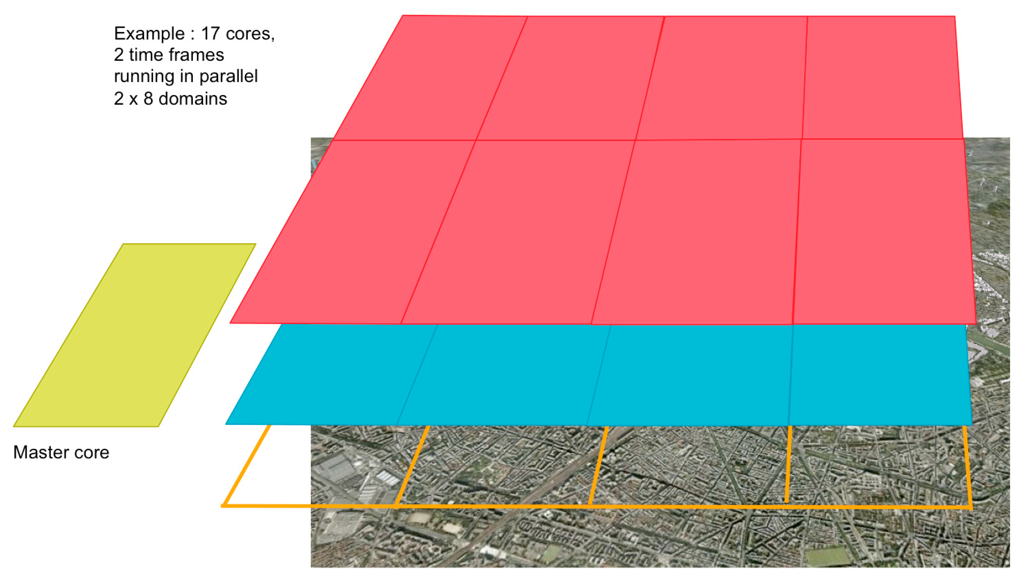
The algorithm uses a master core to distribute the workload and access the input data, like topography, land use, buildings, etc.
Figure 1 displays an example of a calculation using 17 cores: two timeframes are calculated simultaneously and the domain is divided into 8 tiles.
A dispersion calculation performed by the PSPRAY model can also be parallelized in two ways using:
- DD, essentially to handle weak scaling issues. DD is inherited from PSWIFT,
- Particle Decomposition (PD), essentially to handle strong scaling and reduce the computational time of a given calculation. PD uses the Lagrangian property of the code: each particle is independent, except for Eulerian processes.
PD requires few communications, similarly to TD for the PSWIFT model. In contrast, DD implies numerous MPI exchanges. Indeed, particles that move across a tile boundary are exchanged between cores on each side of the boundary. This action is performed at each synchronization time step. The synchronization time step is used by Lagrangian models to compute the concentration on the calculation grid: all particles are moved until a synchronization time step occurs to make sure their positions are known at exactly the same moment, making the concentration calculation possible.
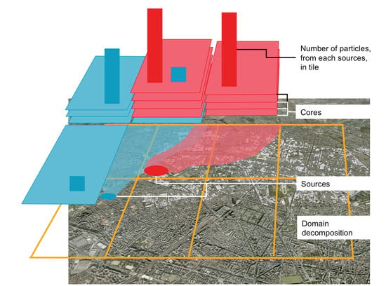
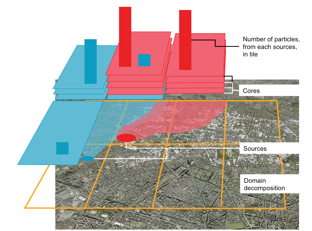
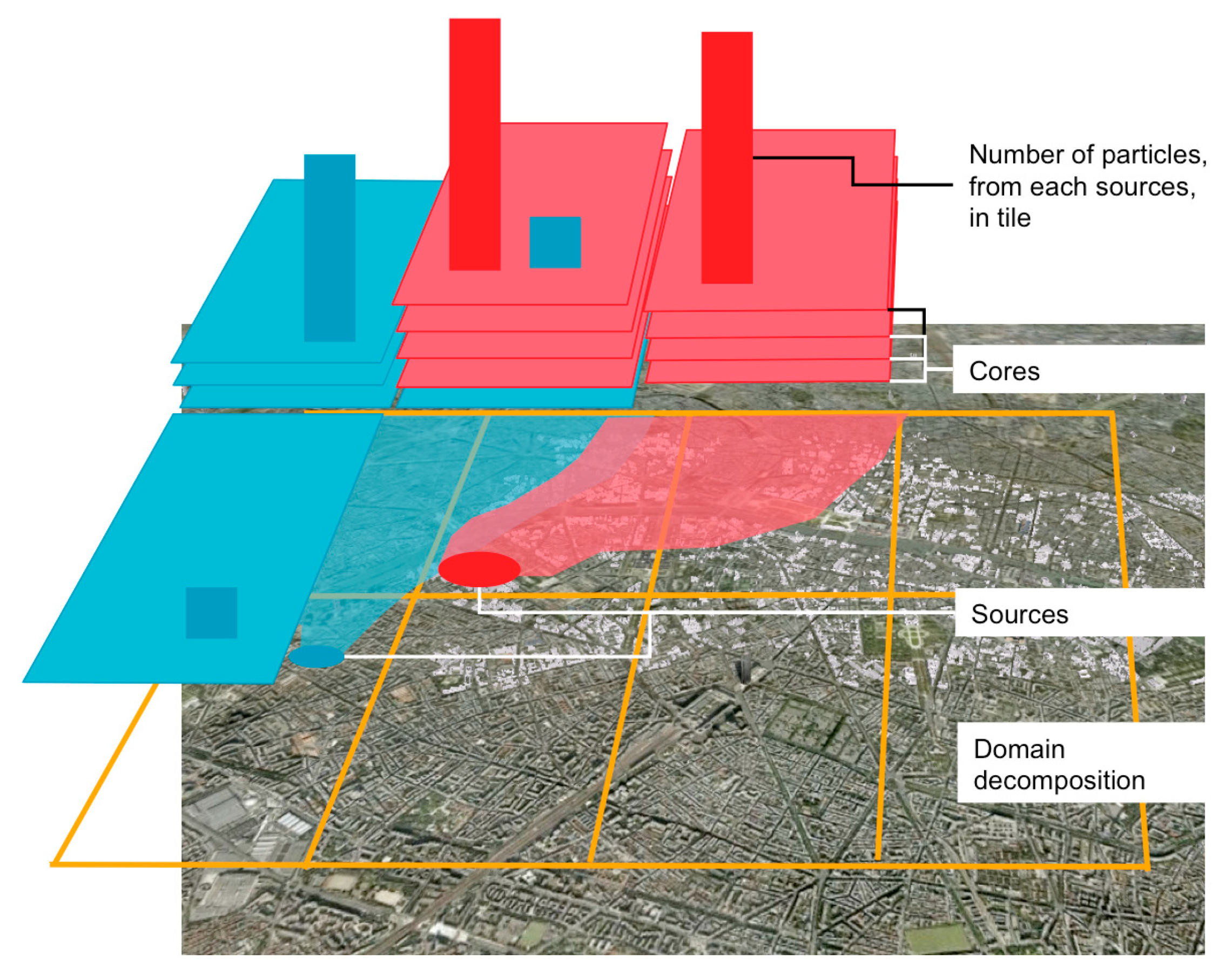
DD is more complex for Lagrangian models than it is for Eulerian models like PSWIFT. Indeed, computational cores are not distributed evenly between tiles. In principle, the more the particles are in a tile, the more cores are allocated to this tile. Since the number of particles per tile is evolving drastically in the case of transient plume, the allocation of cores on tiles is also changing. This is called Load Balancing (LB) and performed by the master core.
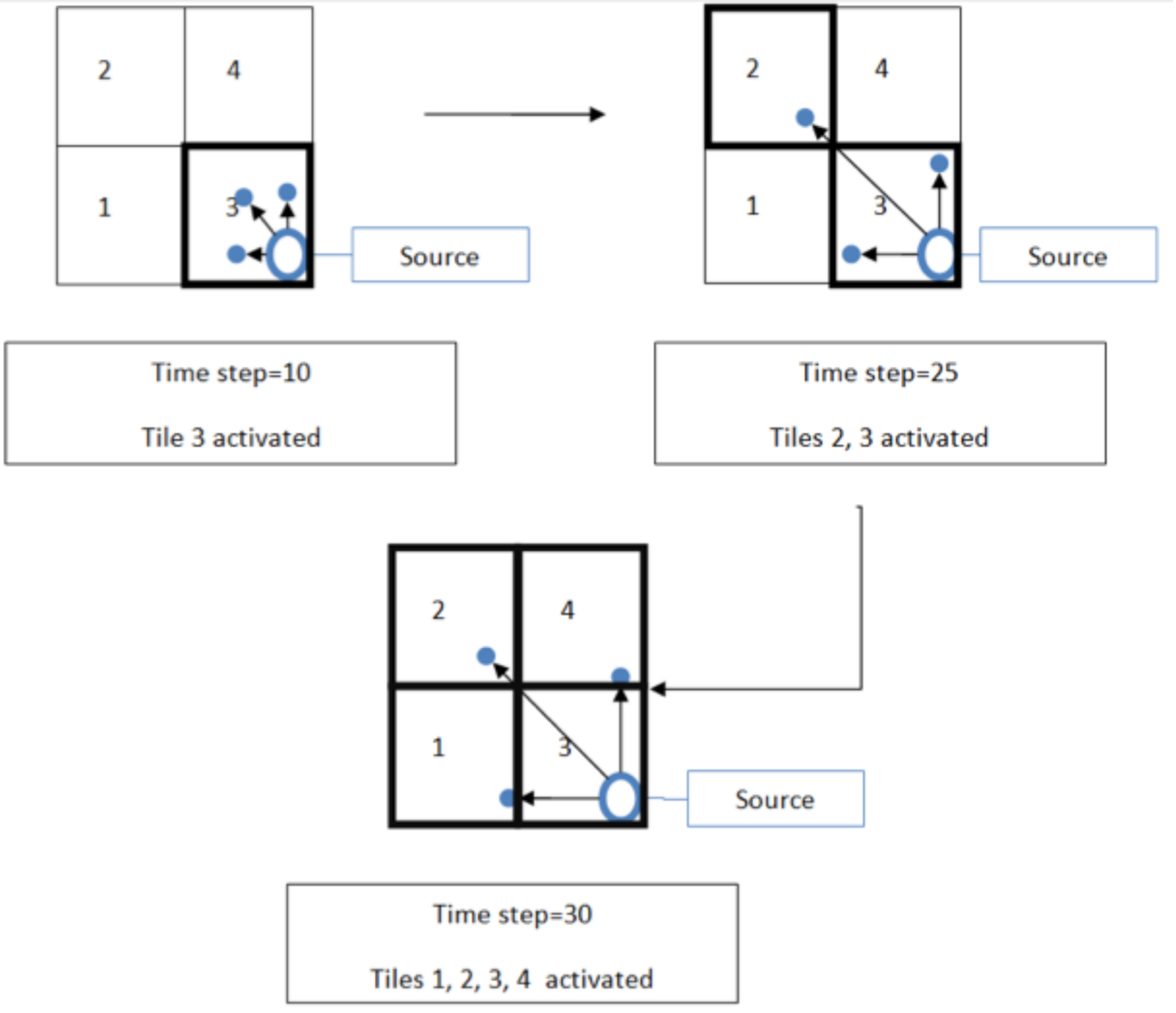
Figure 2 illustrates the process of tiles activation for a domain decomposed in 4 tiles and Figure 3 gives an instantaneous LB for the domain decomposed in 8 tiles, used above as an example for PSWIFT.
LB occurs automatically when required by the plume evolution, what corresponds to particles reaching new parts of the calculation domain. It is referred to as automatic LB from now on. LB can additionally be scheduled by the user on a regular basis to favor a better regular redistribution of the computational resources. This LB is referred to as scheduled LB.
Up to now, the efficiency of PMSS parallel algorithms has been evaluated mostly for TD, for the PSWIFT model, and for PD, for the PSPRAY model [1,23]. No test cases of the DD efficiency were realized, except for some tests performed in the framework of the AIRCITY project [35]. The AIRCITY project was dedicated to modeling the air quality in Paris, France, using a large calculation domain and a fine grid resolution. The calculation domain was covering an area of 12 × 10 km, encompassing Paris city, at a horizontal grid resolution of 3 m. Efficiency of the DD was tested solely for PSWIFT. The number of cores used in these tests ranged from 10 up to 701.
This work focuses on the sole evaluation of the DD parallel algorithm conceived to allow calculation on extremely large calculation domains at high horizontal grid resolution (of around 1 meter).
3. Model Setup for the EMED Project
The evaluation of DD parallel algorithm for the whole PMSS modeling system was realized in the framework of the Emergencies—MEDiterranean sea (EMED) project [22]. Indeed, the size of the calculation grid was very large and allowed to test the algorithms up to more than 8000 cores of a High Performance Computing center.
After presenting the EMED project and the scenario used for the evaluation, the configurations of the calculations are described.
3.1. The EMED Project
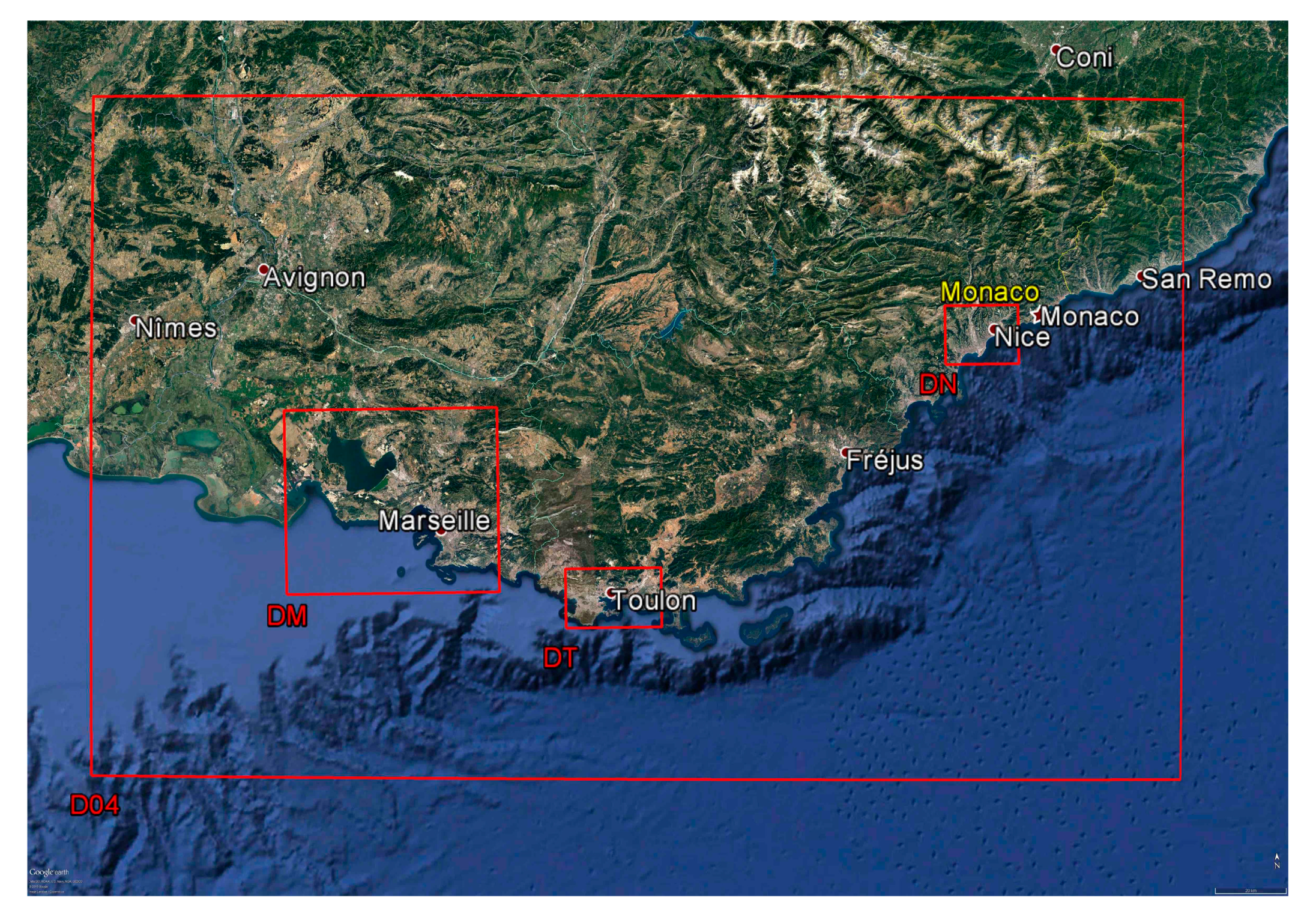
The EMED project was performed in 2016 as a follow-up of the EMERGENCIES project [36]. The EMERGENCIES project was launched in 2014 to demonstrate the feasibility to perform 4D (4-dimensional) numerical simulations as a support tool for decision-making in an emergency situation. The modeled area was the territory under responsibility of the Fire Brigade of Paris and covered an area of 40 by 40 km. The EMED project was dedicated to deploy the PMSS modeling system on another very large area along a large part of the French Mediterranean coast with high resolution nested domains centered on the largest cities of this region (Marseille, Toulon and Nice).
Meteorological forecast from the meso-scale to the local scale and dispersion simulations of fictive releases were performed using the PMSS modeling system nested within Weather Research and Forecast (WRF, see reference [37]) model calculations and accounting for all buildings in the urban domains. Figure 4 presents an overview of the most inner WRF domain and the three nested domains used by the PMSS modeling system.
The scenario retained by the EMED project for the PMSS modeling system consisted in:
- Routine calculation using PSWIFT flow model on the nested domains with a horizontal grid step of 3 m, using WRF meteorological forecasts as input data. These calculations were performed for 24 h with timeframes of every 15 min. The WRF horizontal grid step was 1 km.
- On-demand calculations using PSPRAY dispersion model in case of accidental or malevolent releases and the PSWIFT flow predictions. In the project, we considered fictive releases.
The domain largely encompassing the city of Marseille and the associated PMSS calculations are now commented on.
3.2. Configurations of the Calculations and of the Computing Cluster
The calculation grid of Marseille and its vicinity has a horizontal footprint of 58 by 50 km. The grid step is 3 m horizontally and 1m in the first vertical levels. The grid has 39 vertical levels and 19,333 × 16,666 vertices horizontally, hence more than 12.5 billion nodes.
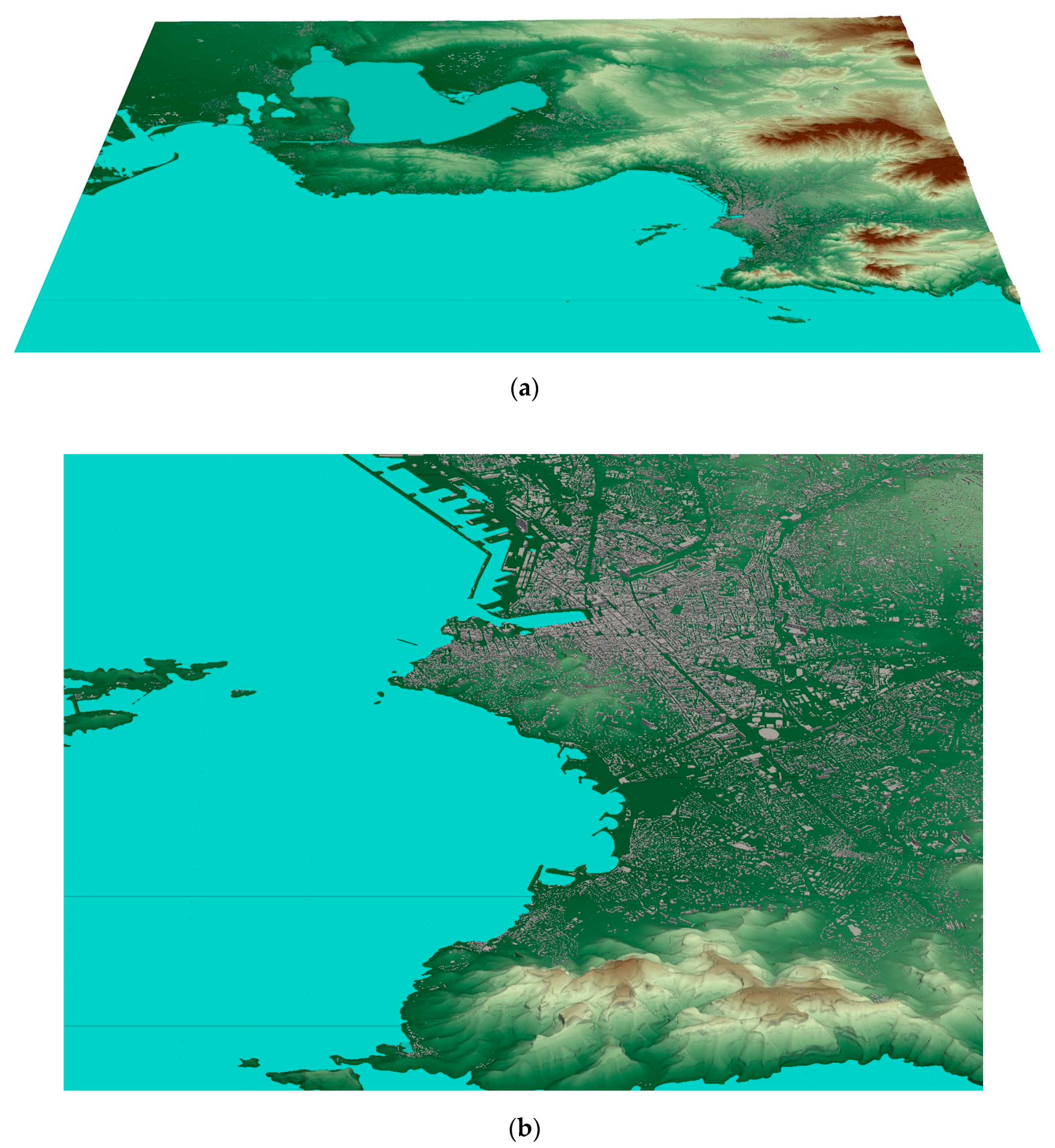
The topography originates from the French Geographic Institute (IGN) with a resolution of 5 m. The data are interpolated at the calculation grid resolution. The landscape has stiff slopes and an amplitude of roughly 1000 m. The model input file has a disk footprint of 6.5 GB.
The building data also originates from the IGN. The model input file has a disk footprint of 400 MB.
Figure 5 shows an overview of the topography of the domain, including the buildings, with a zoom on the city of Marseille. The city of Marseille is located along the coast, looking westward, on the right hand side of the picture. The domain encompasses the coastal lagoon Étang de Berre, located on the left hand side on the top part of the image. On the shores of the Étang de Berre, and along the coast nearby, stand a lot of industrial facilities docks.
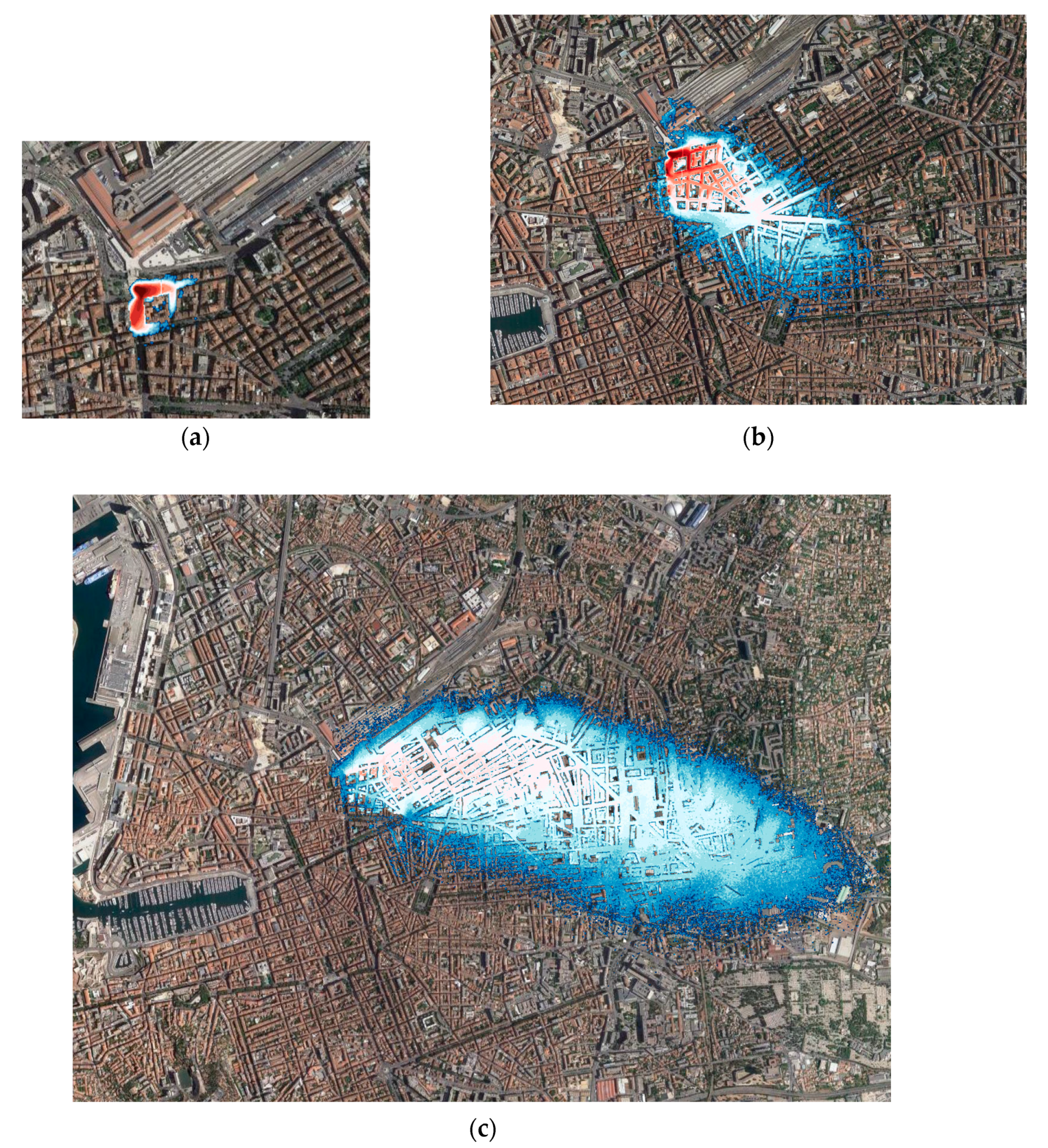
The duration of the dispersion simulation is 4 h between 19:00 and 23:00 (local time) of the 10th of August 2016. The fictive emissions retained for the scenario consists of four accidental or malevolent releases of hazardous materials located in the vicinity of public buildings or industrial plants. The duration of each release is 20 min. The releases started at 19:00, 19:30, 20:00 and 20:30.
Figure 6 shows the deleterious plume, which originated from one of the four malevolent releases, this one near the central train station, 3 min, 15 min, and 1 h after the beginning of the release.
PSPRAY uses a synchronization time step of 5 s. The settings chosen for dispersion were driven to obtain a very detailed plume evolution, certainly more than required in the framework of urgency. Hence, the following parameterization:
- Concentrations are calculated every minute using 12 samples taken every 5 s;
- 400,000 numerical particles are emitted every 5 s during the release periods. Hence 384 millions of numerical particles are emitted during the whole simulation. This number is very large and was chosen to allow for the computation of concentration each and every minute.
User defined LB is scheduled every 10 min as a tradeoff between:
- Performing the LB too often, and getting too many LB additional computing costs implying notably loading and unloading flow data, sending and receiving particles;
- Not performing the LB, and having inefficient setup of cores on the domain, with respect to the locations of the particles.
Calculations were performed on a Bull-X supercomputer with 39,816 Intel Xeon cores, clocked at 2.4 GHz, gathered in nodes of 28 cores with 128 GB of memory. Note that not all of the cores were made available for the EMED project.
The PMSS modeling system requires several hundreds or thousands of computing cores for the EMED project because of the size of the responsibility areas of the emergency teams, and the high-resolution metric grid step used. If the modeling system is applied to an industrial facility, a public building, or an urban district of a few square kilometers, calculation times compatible with crisis management can be obtained with 4 to 20 computing cores.
4. Domain Decomposition for the PMSS Modeling System on EMED Project
The following sub-sections present the parallel setup of the flow and dispersion computations over the Marseille simulation domain and discuss the results according to the efficiency of the parallelization using DD.
4.1. DD for the PSWIFT Flow Model
This sub-section describes first the setup, and then the results obtained in terms of parallelization efficiency of the PSWIFT flow computations.
4.1.1. DD Setup
The PSWIFT model uses a finite difference discretization on the grid. As described above, the EMED grid has 19,333 per 16,666 vertices horizontally, and 39 along the vertical.
The size of the EMED grid made it possible to test the DD up to the maximum grid size allowed in RAM memory, without caching, for a single core. The tiles used for the domain decomposition had a size from 201 × 201 up to 1001 × 1001 horizontal vertices, with 39 levels along the vertical.
Table 1 shows all DD configuration tested on the Bull-X supercomputer. The number of computing cores is equal to the number of tiles plus the master core.
The case of tile with 101 × 101 points was not tested since it required 31,872 cores, which is more than the number of cores on the supercomputer allowed in the frame of the project.
4.1.2. DD Results
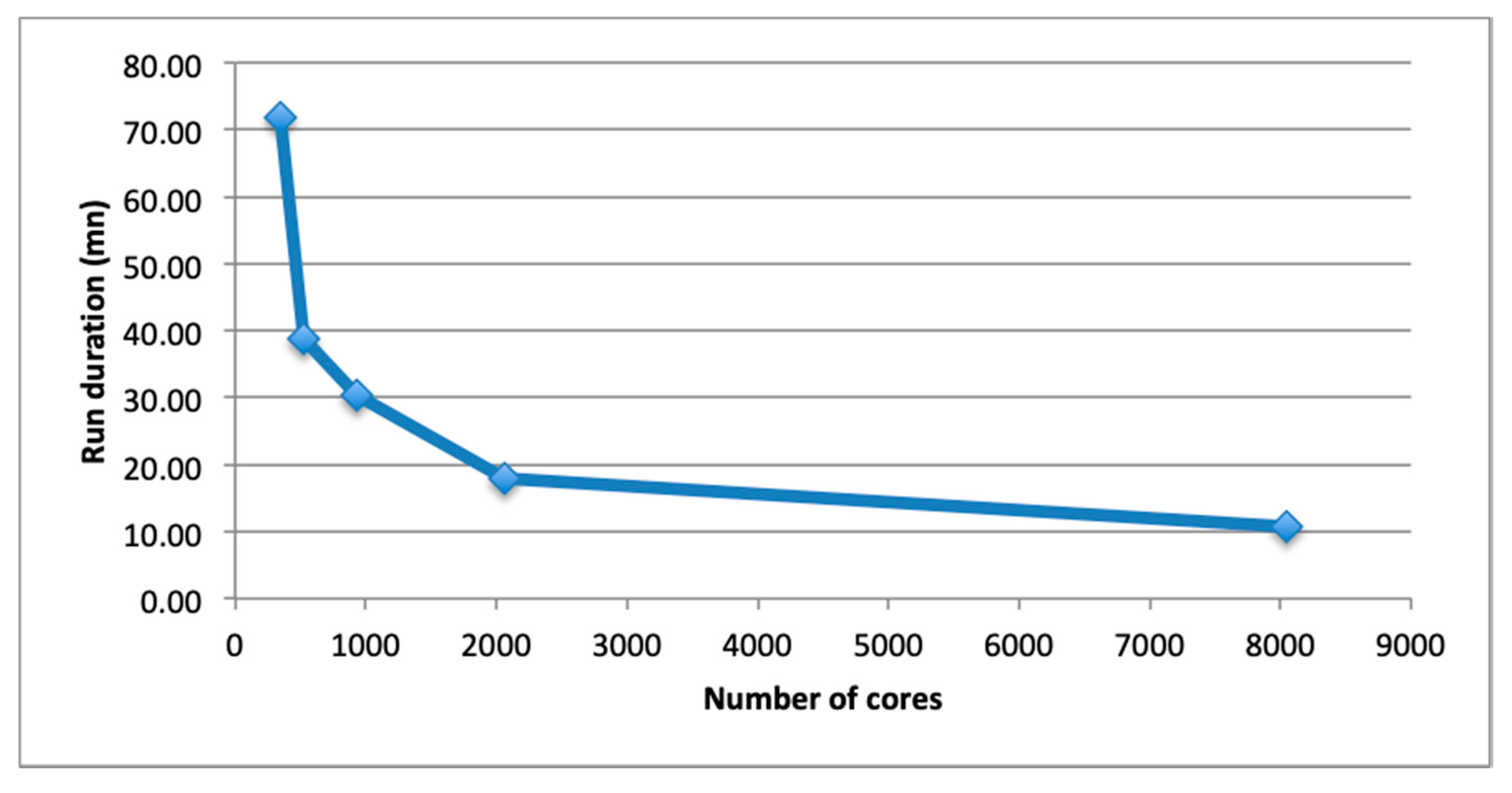
Table 2 shows the calculation durations of a single and 24 timeframes for the various DD presented above. While the timeframes were every 15 min in the EMED project, they could have been computed every hour, so that 24 timeframes would correspond to 1 day of micro-meteorological analysis or forecast.
Figure 7 shows these results on a graph.
The duration to compute a timeframe drops from slightly more than 1 h down to 10 min when the number of cores goes from 300 to 8000 cores.
4.1.3. Discussion
In the framework of a system usable for crisis management, at least 24 pre-computed hourly timeframes of the PMSS local scale flow are expected to be predicted from one day to another. As seen in Table 2, for the EMED computation domain over Marseille, no more than 500 cores are necessary to predict the local urban flow at high resolution one day in advance.
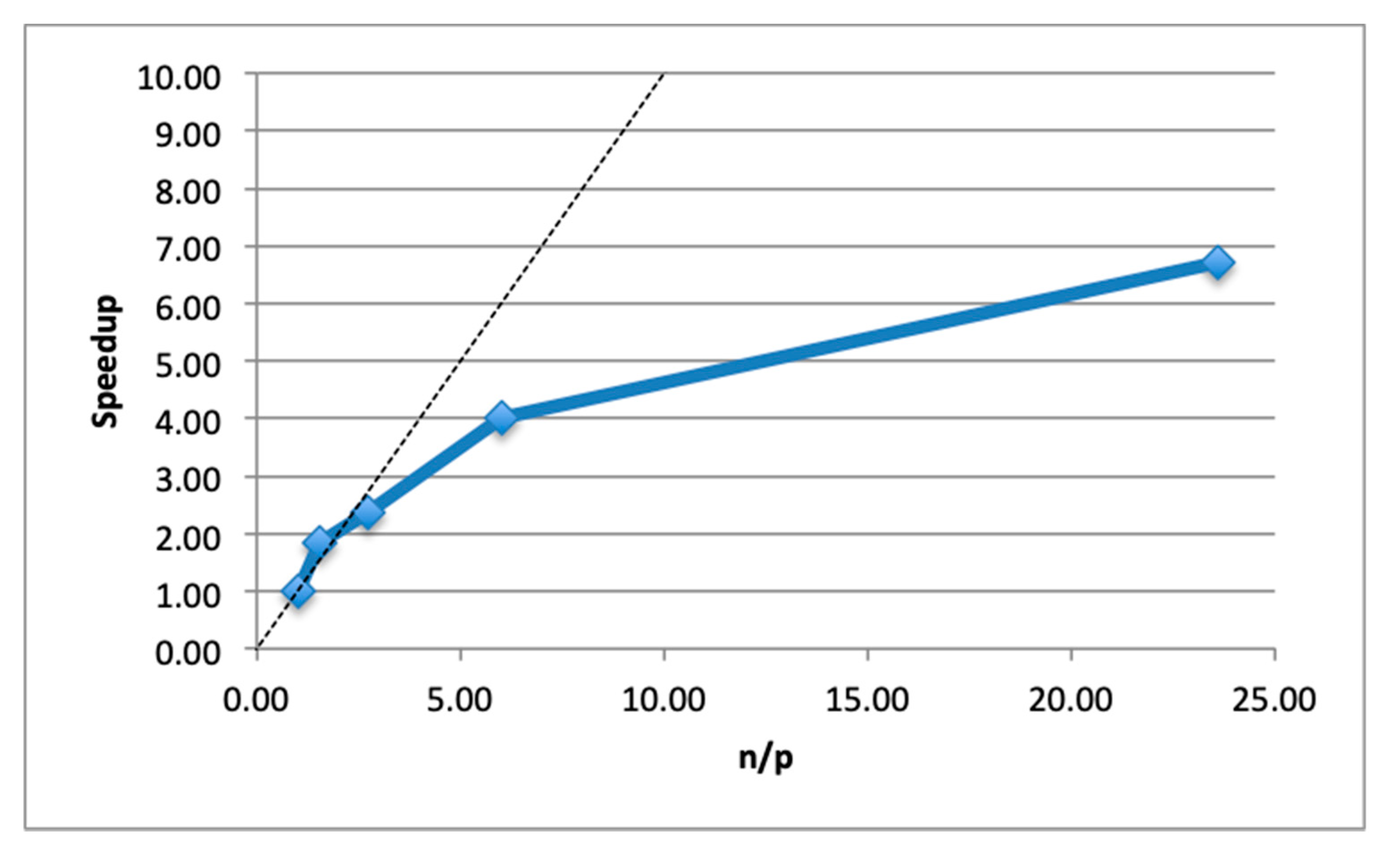
The speedup S(n) for n cores is defined as the ratio the reference duration using p cores, Tp, here p = 341, divided by the duration using n cores, Tn:
S(n) = Tp/Tn,
In EMED, 341 cores are required for the reference case, as it was not possible to compute the flow on less than 340 cores given the size of the high-resolution domain over Marseille and vicinity. Figure 8 displays the speedup as a function of the ratio n/p.
The ideal speedup (IS), is obtained when multiplying the number of cores by x lead to a duration of 1/xth of the run duration, hence a speedup multiplied by ×. It follows that:
IS(n/p) = n/p,
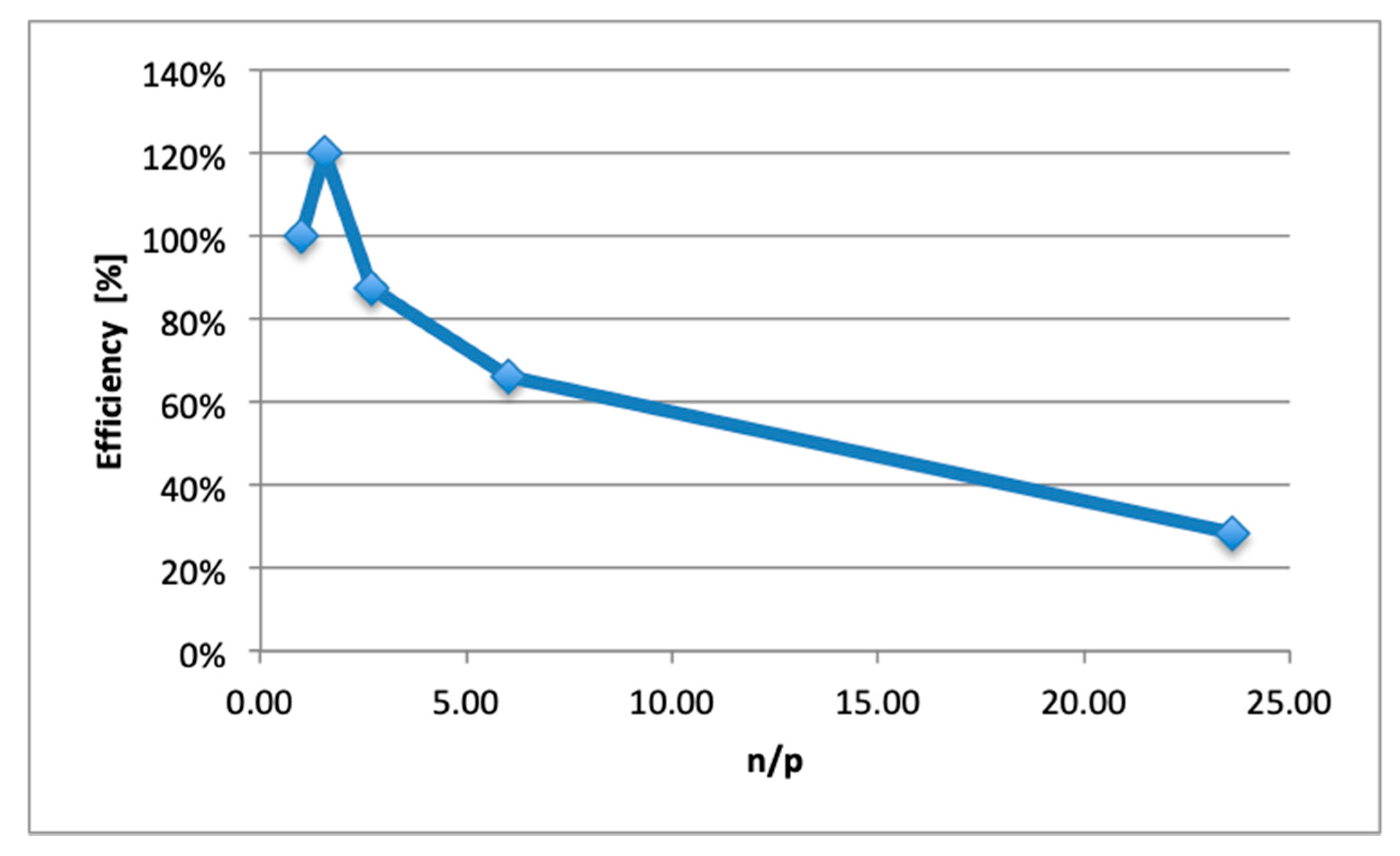
The efficiency E is defined as the ratio of the speedup divided by the ideal speedup:
E = S/IS = p Tp/(n Tn),
For instance, an efficiency of 50% means than only 50% of the ideal speed-up is obtained. Since the speedup is limited for instance by Amdahl’s law [38], and as IS is linear, efficiency tends towards 0 as n tends to infinity.
Figure 9 shows the efficiency as a function of ratio n/p. The efficiency decreases when n/p is above 3, i.e., around 1000 cores, and drops below 50% for n/p above 14, i.e., around 4700 cores.
The efficiency of n/p around 2 is better than the reference case. It is explained by the decrease of computational time due to a better LB overcompensating the increase of parallelization extra costs (such as communications) using 526 cores compared to 341 cores.
On the EMED project, the DD retained for the project used 2058 tiles of individual dimensions 401 × 401. That DD was thus a good compromise for a typical operational crisis setup:
- The efficiency remained still above 50% of the minimal setup to be able to run the calculation on the supercomputer;
- The local scale flow simulation duration took less than 20 min for a timeframe calculation, allowing the prediction of the minimum 24 timeframes in around 7 h.
4.2. DD for the PSPRAY Dispersion Model
This sub-section describes first the setup, and then the results obtained in terms of parallelization efficiency of the PSPRAY dispersion computations.
4.2.1. DD Setup
The DD study regarding the PSPRAY model in the PMSS modeling system inherits the DD studied for the PSWIFT model. Nonetheless, and due to the Lagrangian nature of the model, the number of cores required to run a specific DD is not related to the number of tiles in the domain, but instead to the maximum number of tiles used simultaneously.
The DD tests were performed:
- On all the DD defined for PSWIFT: 340, 525, 924, 2058 and 8051 tiles,
- With a number of 500, 1000, 1500 and 3000 cores.
The tests were then evaluated in two ways:
- The influence of the number of cores on a given DD,
- The influence of the DD on a given number of cores.
4.2.2. DD Results
Table 3 displays the duration of the calculation according to the number of cores and number of tiles (in hh:mn:ss).
The configuration using 340 tiles, with dimension of 1001 × 1001 points required too much memory, except when using 3000 cores. It is consistent with the memory constraint of PSWIFT where 1001 tends to be the limit for RAM usage since PSPRAY loads two timeframes, hence providing almost twice the flow arrays of the PSWFIT model, plus the particle arrays. Indeed, the PSPRAY model interpolates the flow properties between two timeframes of the flow.
The best speedup is achieved using the finest DD tested (8051 tiles) and 3000 cores.
4.2.3. Discussion on the Influence of the DD
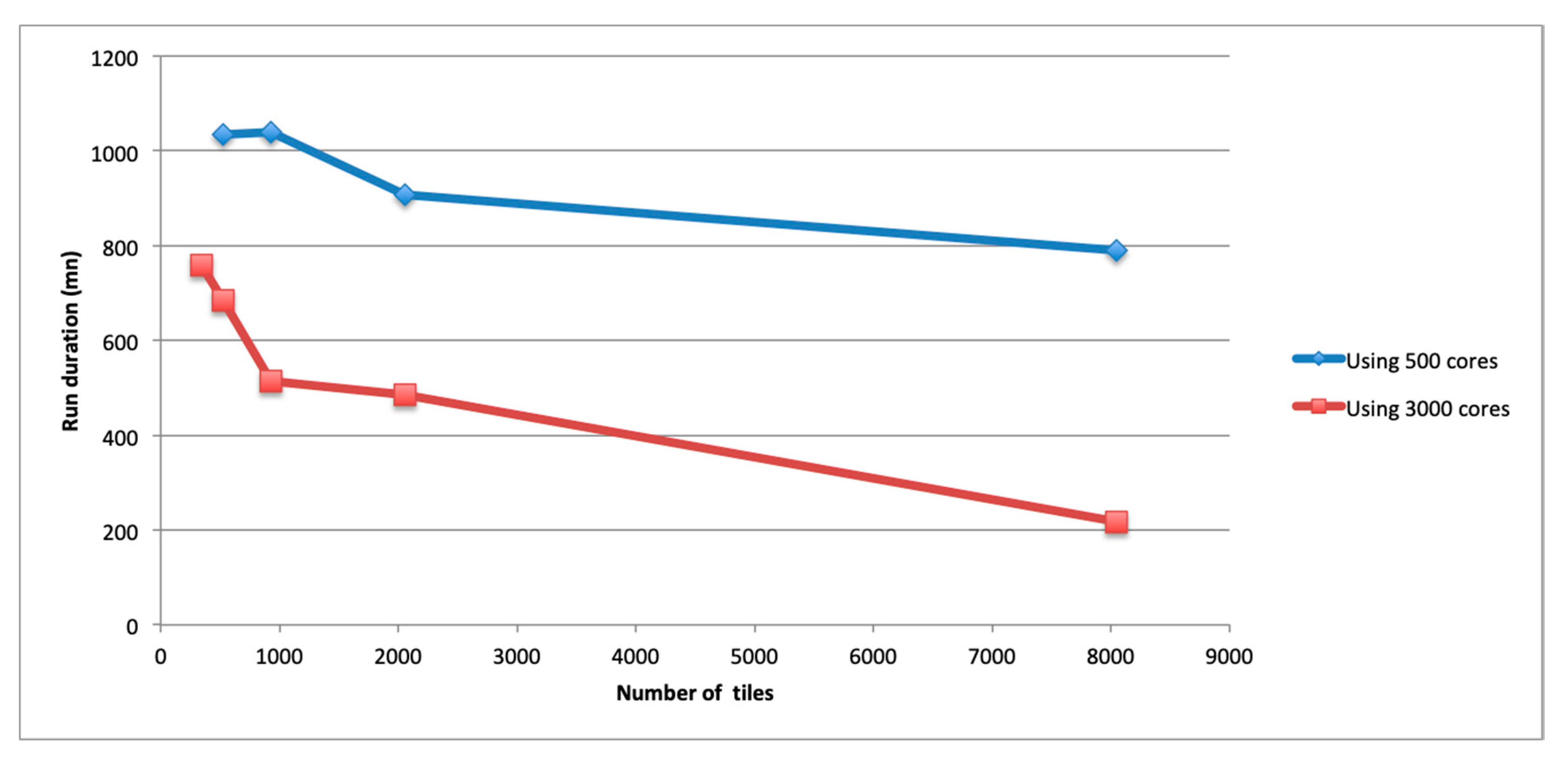
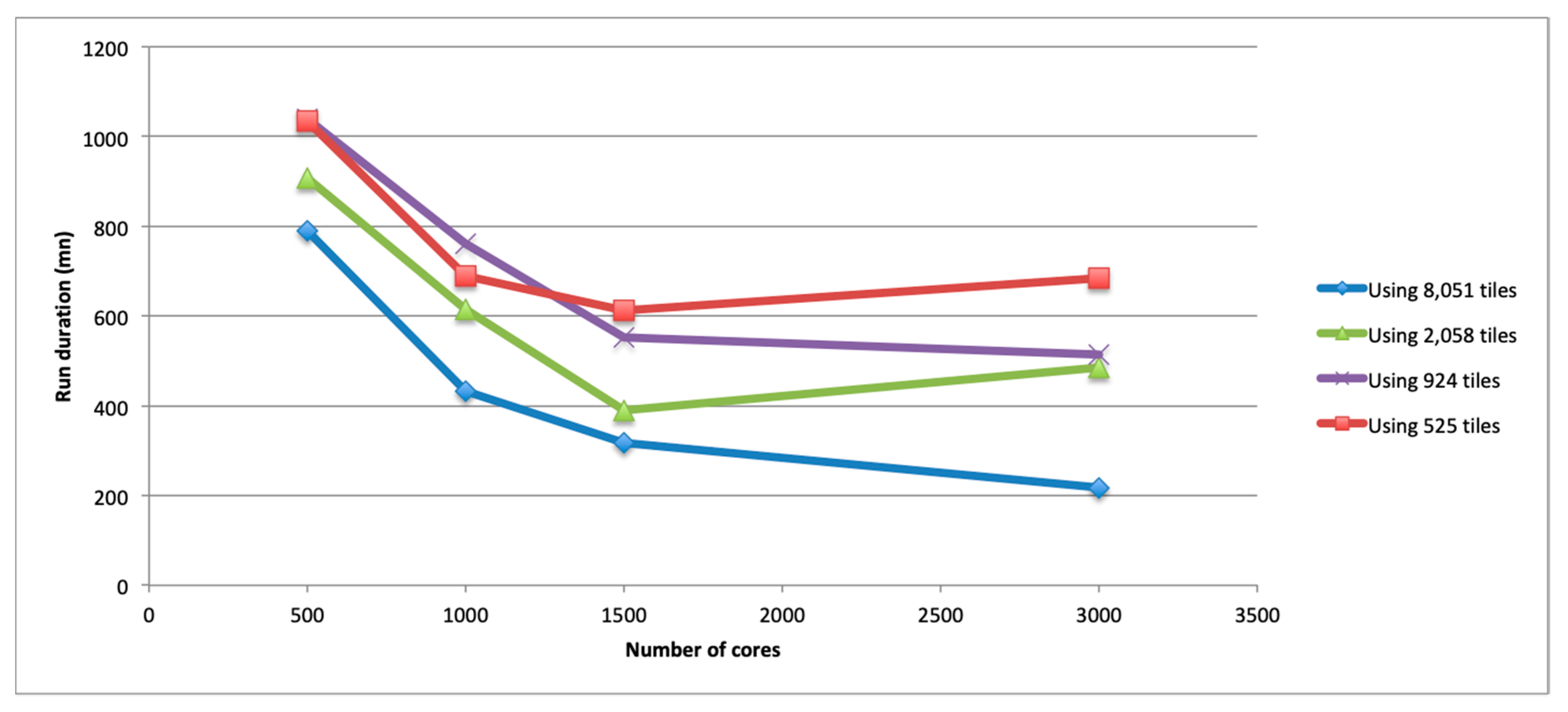
Figure 10 displays the evolution of the simulation duration as a function of the number of tiles of the DD, when using 500 and 3000 cores.
Figure 10 raises three major comments, the two latest being discussed afterwards:
- As expected, the run duration is the shortest when using 3000 cores;
- The finer the DD, the shorter the run duration is;
- Reducing the number of tiles in the DD decomposition reduces the impact of using more computing cores.
The third comment amounts to saying that, when the DD uses few tiles, the run duration tends to be more similar no matter the number of cores being used. This trend is confirmed by the run duration considering 1000 or 1500 cores, around 11 h, the same order of magnitude as for 3000 cores.
This can be related to the propagation of the plume and the automatic LB: each time particles are reaching a new tile, then a core is dedicated to that new tile. If a large amount of particles are reaching later on that tile before the next scheduled LB, then only this single core is used to handle that large amount of particles. Hence, the whole calculation is slowed by the core dedicated to that particular tile, independently of the number of cores used for the whole calculation. This phenomenon is named Single Core Before LB (SCBLB).
Indeed, new tiles are activated less often when using larger tiles: they are less numerous and particles are taking more time to get through them. Therefore, automatic LB occurs less frequently the larger the tiles. Moreover, and due to the size of the tiles, larger amount of particles can reach the tile before the next scheduled or automatic LB.
When using more tiles for the DD, computation time is decreasing in spite of more communications being required. A similar process as described before is under way. When increasing the number of tiles, hence reducing their area, automatic LB is performed more often, and at a frequency more closely related to the propagation of the plume. Therefore the LB is intrinsically optimized. Moreover, SCBLB effect is also more limited.
4.2.4. Discussion on the Influence of the Number of Cores
Figure 11 shows the duration of the calculations as a function of the number of cores used, and for the various DD.
Figure 11 shows that:
- Consistently with the previous section, a finer DD generally shortens the duration of the simulation.
- More computing cores reduce the simulation duration up to the point where the additional cost of LB more than compensate the gain in computing power.
For up to 1500 cores, adding more computing power allows us to decrease the simulation duration. But after that limit, the algorithm used to distribute the workload suffers from bottlenecks related to the handling of LB by the master core.
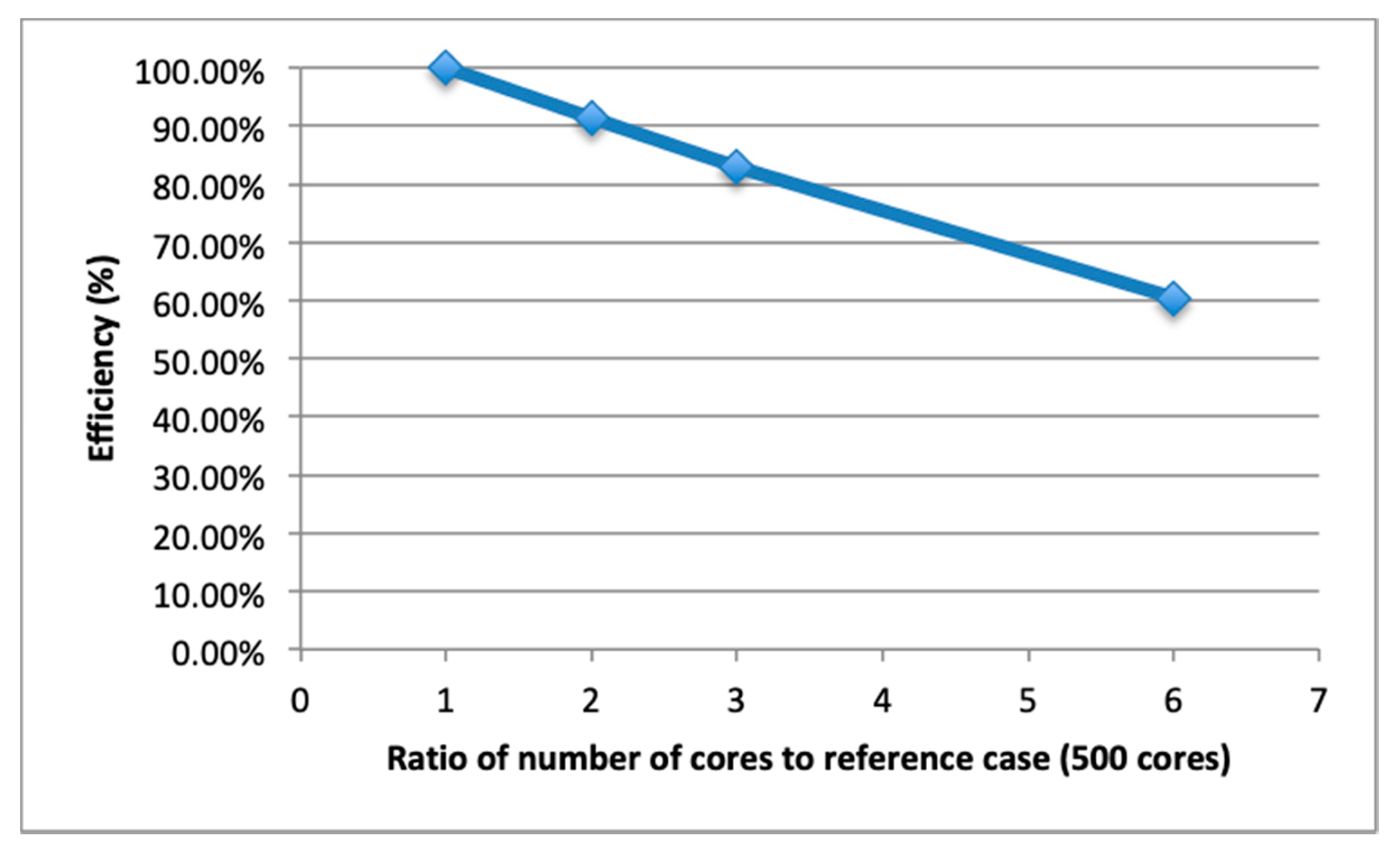
Figure 12 shows the efficiency curve for the DD using 8051 tiles. The test case using 500 cores is used as a reference case.
In the 500 to 3000 cores range, we can see that the efficiency remains above 50%.
As discussed in Section 3.2, this sensitivity study on the PSPRAY model was performed using a very large number of particles. For a calculation solely dedicated to crisis management, concentrations would be calculated using 10 min averages and using 40,000 particles emitted every 5 s, instead of 400,000 particles and 1 min averages. Using these settings and 1000 cores with the 2051 tiles configuration, the simulation drops to 30 min for a plume propagating during 4 h of simulated time. Thus, the calculation is accelerated by a factor of eight compared to the time of the physical process.
5. Conclusions
The sensitivity of the PMSS modeling system to the Domain Decomposition (DD) was studied in the framework of the EMED project, as this project was based on an extremely large urban domain at a very high resolution. The domain consists of 19,333 × 16,666 × 39 grid nodes with a horizontal grid step of 3 m and a vertical grid step of 1 m near the ground. The horizontal domain has an extension of 58 by 50 km. This very large domain allowed testing of the DD from 340 tiles of 1001 × 1001 points up to 8051 tiles of 201 × 201 points.
The PSWIFT flow model shows good performances compared to the reference case using 341 tiles, keeping the efficiency above 50% for up to roughly 4700 cores. 2051 tiles is the best trade-off for the EMED test case, since it allows computing a timeframe in less than 20 min with an efficiency of above 60%. Time Decomposition (TD) also provides the capability to simultaneously run timeframes should additional groups of 2051 cores be available.
The PSPRAY dispersion model shows good performances especially considering that DD implies Load Balancing (LB) to attribute the cores from tile to tile as the plume spreads and moves across the domain. PSPRAY was tested using from 500 to 3000 cores on the various DD. The number of particles and concentration field calculations were chosen to get very detailed plume evolution for the demonstration of the EMED project. The best performances were achieved for the finest DD due to the intrinsically better influence of automatic LB. When using the 8051 tiles and 3000 cores, the simulation duration dropped to 3 h 40 min. When using a less stringent setting of the numerical particles, the simulation duration can be decreased to 30 min with 1000 cores on the 2051 tiles DD. The multiplication of supercomputers all over the world gives access to large numbers of cores (as numerous as many hundreds of thousands for the most recent and foreseen machines). 1000 or 2000 cores, while constituting a large computational resource, are an increasingly available resource for practical operational forecasts.
The calculation domain used in EMED project is especially relevant to crisis management since it is consistent with the responsibility area of the local emergency response authorities. This sensitivity study of DD on the EMED project demonstrates the capability of the PMSS modeling system as an important asset for emergency response applications.
Author Contributions
Conceptualization & Methodology, O.O. and P.A.; Software, O.O. and S.P.; Formal Analysis, O.O.; Investigation, O.O.; Data Curation, O.O., S.P. and C.D.; Writing-Original Draft Preparation, O.O. And P.A.; Writing-Review & Editing, O.O. and P.A.; Visualization, O.O., S.P. and C.D.
Funding
This research received no external funding.
Conflicts of Interest
The authors declare no conflict of interest.
References
- Oldrini, O.; Armand, P.; Duchenne, C.; Olry, C.; Moussafir, J.; Tinarelli, G. Description and preliminary validation of the PMSS fast response parallel atmospheric flow and dispersion solver in complex built-up areas. Environ. Fluid Mech. 2017, 17, 997–1014. [Google Scholar] [CrossRef]
- Armand, P.; Bartzis, J.; Baumann-Stanzer, K.; Bemporad, E.; Evertz, S.; Gariazzo, C.; Gerbec, M.; Herring, S.; Karppinen, A.; Lacome, J.M.; et al. Best Practice Guidelines for the Use of the Atmospheric Dispersion Models in Emergency Response Tools at Local-Scale in Case of Hazmat Releases into the Air. Technical Report COST Action ES 1006. 2015. Available online: http://elizas.eu/images/Documents/Best%20Practice%20Guidelines_web.pdf (accessed on 6 July 2019).
- Oldrini, O.; Armand, P. Validation and Sensitivity Study of the PMSS Modelling System for Puff Releases in the Joint Urban 2003 Field Experiment. Bound. Layer Meteorol. 2019. [Google Scholar] [CrossRef]
- McHugh, C.A.; Carruthers, D.J.; Edmunds, H.A. ADMS-Urban: An air quality management system for traffic, domestic and industrial pollution. Int. J. Environ. Pollut. 1997, 8, 666–674. [Google Scholar]
- Schulman, L.L.; Strimaitis, D.G.; Scire, J.S. Development and evaluation of the PRIME plume rise and building downwash model. J. Air Waste Manag. Assoc. 2000, 5, 378–390. [Google Scholar] [CrossRef]
- Sykes, R.I.; Parker, S.F.; Henn, D.S.; Cerasoli, C.P.; Santos, L.P. PC-SCIPUFF Version 1.3—Technical Documentation. ARAP Report No. 725; Titan Corporation: San Diego, CA, USA, 2000. [Google Scholar]
- Hanna, S.; Baja, E. A simple urban dispersion model tested with tracer data from Oklahoma City and Manhattan. Atmos. Environ. 2009, 43, 778–786. [Google Scholar] [CrossRef]
- Soulhac, L.; Salizzoni, P.; Cierco, F.X.; Perkins, R. The model SIRANE for atmospheric urban pollutant dispersion—Part I: Presentation of the model. Atmos. Environ. 2011, 45, 7379–7395. [Google Scholar] [CrossRef]
- Carpentieri, M.; Salizzoni, P.; Robins, A.; Soulhac, L. Evaluation of a neighbourhood scale, street network dispersion model through comparison with wind tunnel data. Environ. Model. Softw. 2012, 37, 110–124. [Google Scholar] [CrossRef] [Green Version]
- Soulhac, L.; Lamaison, G.; Cierco, F.X.; Ben Salem, N.; Salizzoni, P.; Mejean, P.; Armand, P.; Patryl, L. SIR-ANERISK: Modelling dispersion of steady and unsteady pollutant releases in the urban canopy. Atmos. Environ. 2016, 140, 242–260. [Google Scholar] [CrossRef]
- Camelli, F.E.; Hanna, S.R.; Lohner, R. Simulation of the MUST field experiment using the FEFLO-urban CFD model. In Proceedings of the 5th Symposium on the Urban Environment, American Meteorological Society, Vancouver, BC, Canada, 23–26 August 2004. [Google Scholar]
- Gowardhan, A.A.; Pardyjak, E.R.; Senocak, I.; Brown, M.J. A CFD-based wind solver for an urban fast response transport and dispersion model. Environ. Fluid Mech. 2011, 11, 439–464. [Google Scholar] [CrossRef]
- Gowardhan, A.A.; Pardyjak, E.R.; Senocak, I.; Brown, M.J. Investigation of Reynolds stresses in a 3D idealized urban area using large eddy simulation. In Proceedings of the AMS Seventh Symposium on Urban Environment, San Diego, CA, USA, 26 April 2007. [Google Scholar]
- Kurppa, M.; Hellsten, A.; Auvinen, M.; Raasch, S.; Vesala, T.; Järvi, L. Ventilation and air quality in city blocks using Large Eddy Simulation–Urban planning perspective. Atmosphere 2018, 9, 65. [Google Scholar] [CrossRef]
- Kristóf, G.; Papp, B. Application of GPU-based Large Eddy Simulation in urban dispersion studies. Atmosphere 2018, 9, 442. [Google Scholar] [CrossRef]
- Röckle, R. Bestimmung der Strömungsverhältnisse im Bereich komplexer Bebauungsstrukturen. Ph.D. Thesis, Techn. Hochschule Darmstadt, Darmstadt, Germany, 1990. [Google Scholar]
- Kaplan, H.; Dinar, N. A Lagrangian dispersion model for calculating concentration distribution within a built-up domain. Atmos. Environ. 1996, 30, 4197–4207. [Google Scholar] [CrossRef]
- Hanna, S.; White, J.; Trolier, J.; Vernot, R.; Brown, M.; Gowardhan, A.; Kaplan, H.; Alexander, Y.; Moussafir, J.; Wang, Y.; et al. Comparisons of JU2003 observations with four diagnostic urban wind flow and Lagrangian particle dispersion models. Atmos. Environ. 2011, 45, 4073–4081. [Google Scholar] [CrossRef]
- Brown, M.J.; Gowardhan, A.A.; Nelson, M.A.; Williams, M.D.; Pardyjak, E.R. QUIC transport and dispersion modelling of two releases from the Joint Urban 2003 field experiment. Int. J. Environ. Pollut. 2013, 52, 263–287. [Google Scholar] [CrossRef]
- Singh, B.; Pardyjak, E.R.; Norgren, A.; Willemsen, P. Accelerating urban fast response Lagrangian dispersion simulations using inexpensive graphics processor parallelism. Environ. Model. Softw. 2011, 26, 739–750. [Google Scholar] [CrossRef]
- Pinheiro, A.; Desterro, F.; Santos, M.C.; Pereira, C.M.; Schirru, R. GPU-based implementation of a diagnostic wind field model used in real-time prediction of atmospheric dispersion of radionuclides. Prog. Nucl. Energy 2017, 100, 146–163. [Google Scholar] [CrossRef]
- Armand, P.; Duchenne, C.; Oldrini, O.; Perdriel, S. Emergencies Mediterranean—A Prospective High Resolution Modelling and Decision-Support System in Case of Adverse Atmospheric Releases Applied to the French Mediterranean Coast. In Proceedings of the 18th International conference on Harmonisation within Atmospheric Dispersion Modeling for Regulatory Purposes, Bologna, Italy, 9–12 October 2017. [Google Scholar]
- Oldrini, O.; Olry, C.; Moussafir, J.; Armand, P.; Duchenne, C. Development of PMSS, the parallel version of Micro-SWIFT-SPRAY. In Proceedings of the 14th International Conference on Harmonisation within Atmospheric Dispersion Modelling for Regulatory Purposes, Kos, Greece, 2–6 October 2011; pp. 443–447. [Google Scholar]
- Tinarelli, G.; Brusasca, G.; Oldrini, O.; Anfossi, D.; Trini Castelli, S.; Moussafir, J. Micro-Swift-Spray (MSS): A new modelling system for the simulation of dispersion at microscale–General description and validation. In Air Poll Modelling and Its Applications, 17th ed.; Borrego, C., Norman, A.N., Eds.; Springer: Dordrecht, The Netherlands, 2007; pp. 449–458. [Google Scholar]
- Oldrini, O.; Nibart, M.; Armand, P.; Olry, C.; Moussafir, J.; Albergel, A. Multi-scale build-up area integration in Parallel SWIFT. In Proceedings of the 15th International Conference on Harmonisation within Atmospheric Dispersion Modeling for Regulatory Purposes, Madrid, Spain, 6–9 May 2013. [Google Scholar]
- Oldrini, O.; Nibart, M.; Armand, P.; Moussafir, J.; Duchenne, C. Development of the parallel version of a CFD-RANS flow model adapted to the fast response in built-up environment. In Proceedings of the 17th International Conference on Harmonisation within Atmospheric Dispersion Modeling for Regulatory Purposes, Budapest, Hungary, 9–12 May 2016. [Google Scholar]
- Moussafir, J.; Oldrini, O.; Tinarelli, G.; Sontowski, J.; Dougherty, C. A new operational approach to deal with dispersion around obstacles: The MSS (Micro-Swift-Spray) software suite. In Proceedings of the 9th International Conference on Harmonisation within Atmospheric Dispersion Modeling for Regulatory Purposes, Garmisch, Germany, 1–4 June 2004. [Google Scholar]
- Oldrini, O.; Nibart, M.; Armand, P.; Olry, C.; Moussafir, J.; Albergel, A. Introduction of momentum equations in Micro-SWIFT. In Proceedings of the 16th International Conference on Harmonisation within Atmospheric Dispersion Modeling for Regulatory Purposes, Varna, Bulgaria, 8–11 September 2014. [Google Scholar]
- Anfossi, D.; Desiato, F.; Tinarelli, G.; Brusasca, G.; Ferrero, E.; Sacchetti, D. TRANSALP 1989 experimental campaign–II Simulation of a tracer experiment with Lagrangian particle models. Atmos. Environ. 1998, 32, 1157–1166. [Google Scholar] [CrossRef]
- Anfossi, D.; Tinarelli, G.; Trini Castelli, S.; Nibart, M.; Olry, C.; Commanay, J. A new Lagrangian particle model for the simulation of dense gas dispersion. Atmos. Environ. 2010, 44, 753–762. [Google Scholar] [CrossRef]
- Tinarelli, G.; Anfossi, D.; Brusasca, G.; Ferrero, E.; Giostra, U.; Morselli, M.G.; Tampieri, F. Lagrangian particle simulation of tracer dispersion in the lee of a schematic two-dimensional hill. J. Appl. Meteorol. 1994, 33, 744–756. [Google Scholar] [CrossRef]
- Tinarelli, G.; Mortarini, L.; Trini Castelli, S.; Carlino, G.; Moussafir, J.; Olry, C.; Armand, P.; Anfossi, D. Review and validation of Micro-Spray, a Lagrangian particle model of turbulent dispersion. Lagrangian Modeling Atmos. 2012, 200, 311–327. [Google Scholar]
- Rodean, H.C. Stochastic Lagrangian Models of Turbulent Diffusion; American Meteorological Society: Boston, MA, USA, 1996. [Google Scholar]
- Thomson, D.J. Criteria for the selection of stochastic models of particle trajectories in turbulent flows. J. Fluid Mech. 1987, 180, 529–556. [Google Scholar] [CrossRef]
- Moussafir, J.; Olry, C.; Nibart, M.; Albergel, A.; Armand, P.; Duchenne, C.; Oldrini, O. AIRCITY: A very high resolution atmospheric dispersion modelling system for Paris. In Proceedings of the ASME 2014 4th Joint US-European Fluids Engineering Division Summer Meeting Collocated with the ASME 2014 12th International Conference on Nanochannels, Microchannels, and Minichannels, Chicago, IL, USA, 3–7 August 2014; American Society of Mechanical Engineers: New York, NY, USA, 2014; p. V01DT28A010. [Google Scholar]
- Oldrini, O.; Perdriel, S.; Nibart, M.; Armand, P.; Duchenne, C.; Moussafir, J. EMERGENCIES–A modelling and decision-support project for the Great Paris in case of an accidental or malicious CBRN-E dispersion. In Proceedings of the 17th International Conference on Harmonisation within Atmospheric Dispersion Modeling for Regulatory Purposes, Budapest, Hungary, 9–12 May 2016. [Google Scholar]
- Skamarock, W.C.; Klemp, J.B.; Dudhia, J.; Gill, D.O.; Barker, D.M.; Wang, W.; Powers, J.G. A Description of the Advanced Research WRF Version 2 (No. NCAR/TN-468+ STR); National Center for Atmospheric Research: Boulder, CO, USA, 2005. [Google Scholar]
- Hill, M.D.; Marty, M.R. Amdahl’s law in the multicore era. Computer 2008, 41, 33–38. [Google Scholar] [CrossRef]
Figure 1.
Example of DD combined with TD using 17 cores on a domain divided in 4 × 2 tiles.

Figure 2.
Tile activation process on a domain divided in 4 tiles.

Figure 3.
LB using 13 cores on a domain divided in 4 × 2 tiles and containing 2 release locations. Colors are related to the source.
Figure 3.
LB using 13 cores on a domain divided in 4 × 2 tiles and containing 2 release locations. Colors are related to the source.

Figure 4.
Overview of the most inner WRF domain and of the 3 nested PMSS domains. From left to right are domains over the cities of Marseille, Toulon and Nice.
Figure 4.
Overview of the most inner WRF domain and of the 3 nested PMSS domains. From left to right are domains over the cities of Marseille, Toulon and Nice.

Figure 5.
(a) Overview of the calculation domain; (b) zoom over the city of Marseille.

Figure 6.
(a) View of one of the plume 3 min after the beginning of one of the four fictive releases, located in the vicinity of the train station; (b) 15 min after the release; (c) 60 min after the release.
Figure 6.
(a) View of one of the plume 3 min after the beginning of one of the four fictive releases, located in the vicinity of the train station; (b) 15 min after the release; (c) 60 min after the release.

Figure 7.
PSWIFT run duration for a single timeframe as a function of the number of cores, i.e., the DD decomposition.
Figure 7.
PSWIFT run duration for a single timeframe as a function of the number of cores, i.e., the DD decomposition.

Figure 8.
PSWIFT speedup as a function of the ratio of number of cores n to the reference case p (341 cores). The ideal speedup is plotted as a dashed line.
Figure 8.
PSWIFT speedup as a function of the ratio of number of cores n to the reference case p (341 cores). The ideal speedup is plotted as a dashed line.

Figure 9.
PSWIFT efficiency as a function of the ratio of number of cores n to the reference case p (341 cores).
Figure 9.
PSWIFT efficiency as a function of the ratio of number of cores n to the reference case p (341 cores).

Figure 10.
PSPRAY run duration as a function of the DD and using 500 or 3000 cores.

Figure 11.
PSPRAY run duration as a function of the number of cores, and for the various DD.

Figure 12.
PSPRAY efficiency as a function of the ratio of number of cores to the reference case (500 cores).
Figure 12.
PSPRAY efficiency as a function of the ratio of number of cores to the reference case (500 cores).


Table 1.
DD configurations.
| Number of Points Per Side of Tile | Number of Tiles | Number of Computing Cores |
|---|---|---|
| 1001 | 20 × 17 = 340 | 341 |
| 801 | 25 × 21 = 525 | 526 |
| 601 | 33 × 28 = 924 | 925 |
| 401 | 49 × 42 = 2058 | 2059 |
| 201 | 97 × 83 = 8051 | 8052 |
Table 2.
Calculation durations for the PSWIFT model.
| Number of Cores | Number of Points Per Side of Tile | Calculation Duration Single Timeframe (HH:mm:ss) | Calculation Duration 24 Timeframes (HH:mm:ss) |
|---|---|---|---|
| 341 | 1001 | 01:11:57 | 28:47 |
| 526 | 801 | 00:38:51 | 15:33 |
| 925 | 601 | 00:30:20 | 12:08 |
| 2059 | 401 | 00:18:00 | 07:12 |
| 8052 | 201 | 00:10:42 | 04:17 |
Table 3.
Calculation durations for the PSPRAY model.
| Cores Tiles | 500 | 1000 | 1500 | 3000 |
|---|---|---|---|---|
| 340 | X | X | X | 12:38:44 |
| 525 | 17:14:23 | 11:29:14 | 10:11:26 | 11:25:20 |
| 924 | 17:18:43 | 12:41:57 | 09:13:32 | 08:33:25 |
| 2058 | 15:07:57 | 10:14:00 | 06:30:01 | 08:04:57 |
| 8051 | 13:10:13 | 07:11:53 | 05:17:13 | 03:37:54 |
© 2019 by the authors. Licensee MDPI, Basel, Switzerland. This article is an open access article distributed under the terms and conditions of the Creative Commons Attribution (CC BY) license (http://creativecommons.org/licenses/by/4.0/).
Share and Cite
MDPI and ACS Style
Oldrini, O.; Armand, P.; Duchenne, C.; Perdriel, S. Parallelization Performances of PMSS Flow and Dispersion Modeling System over a Huge Urban Area. Atmosphere 2019, 10, 404. https://0-doi-org.brum.beds.ac.uk/10.3390/atmos10070404
AMA Style
Oldrini O, Armand P, Duchenne C, Perdriel S. Parallelization Performances of PMSS Flow and Dispersion Modeling System over a Huge Urban Area. Atmosphere. 2019; 10(7):404. https://0-doi-org.brum.beds.ac.uk/10.3390/atmos10070404
Chicago/Turabian StyleOldrini, Oliver, Patrick Armand, Christophe Duchenne, and Sylvie Perdriel. 2019. "Parallelization Performances of PMSS Flow and Dispersion Modeling System over a Huge Urban Area" Atmosphere 10, no. 7: 404. https://0-doi-org.brum.beds.ac.uk/10.3390/atmos10070404
Note that from the first issue of 2016, this journal uses article numbers instead of page numbers. See further details here.