Passive Sampling as a Low-Cost Method for Monitoring Air Pollutants in the Baikal Region (Eastern Siberia)


Abstract
:1. Introduction
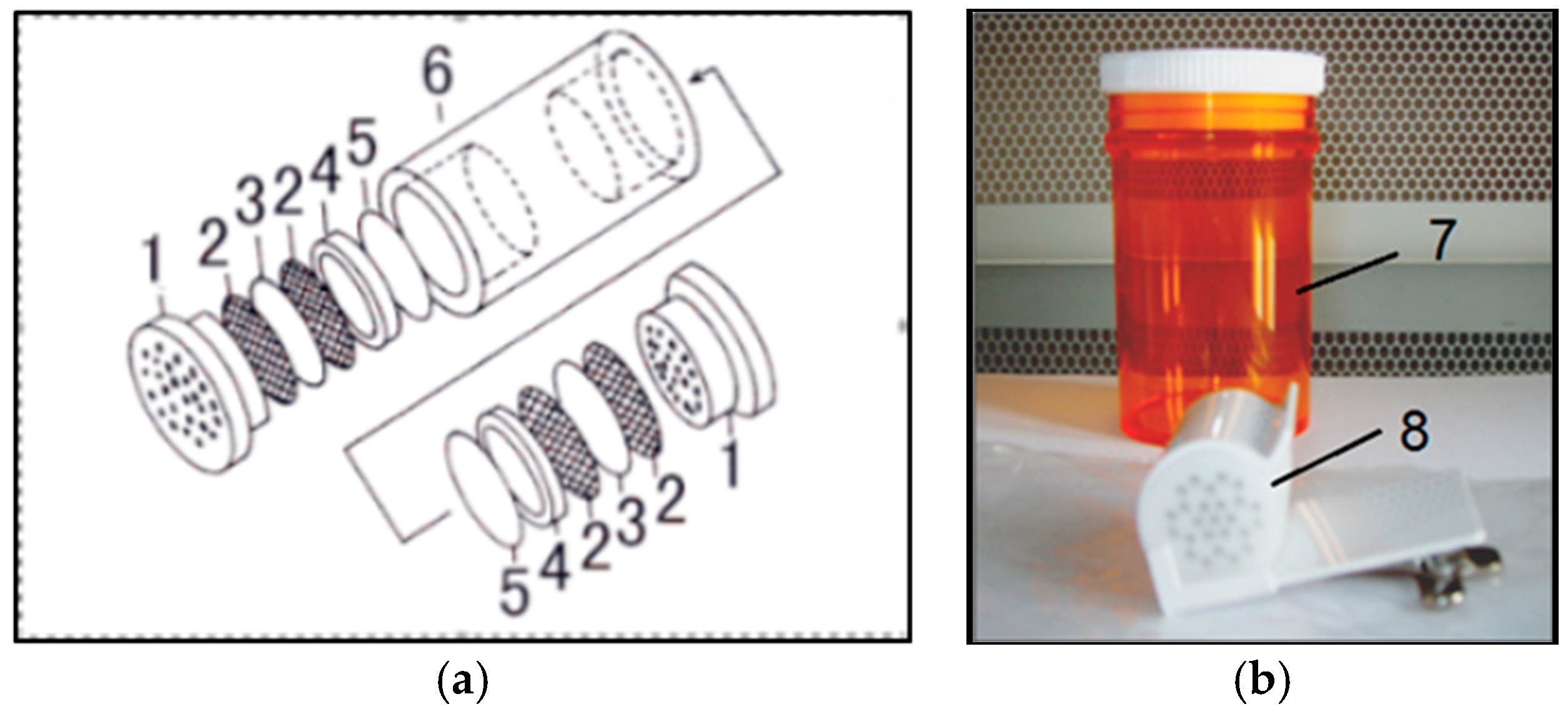
2. Experiments
3. Results and Discussion
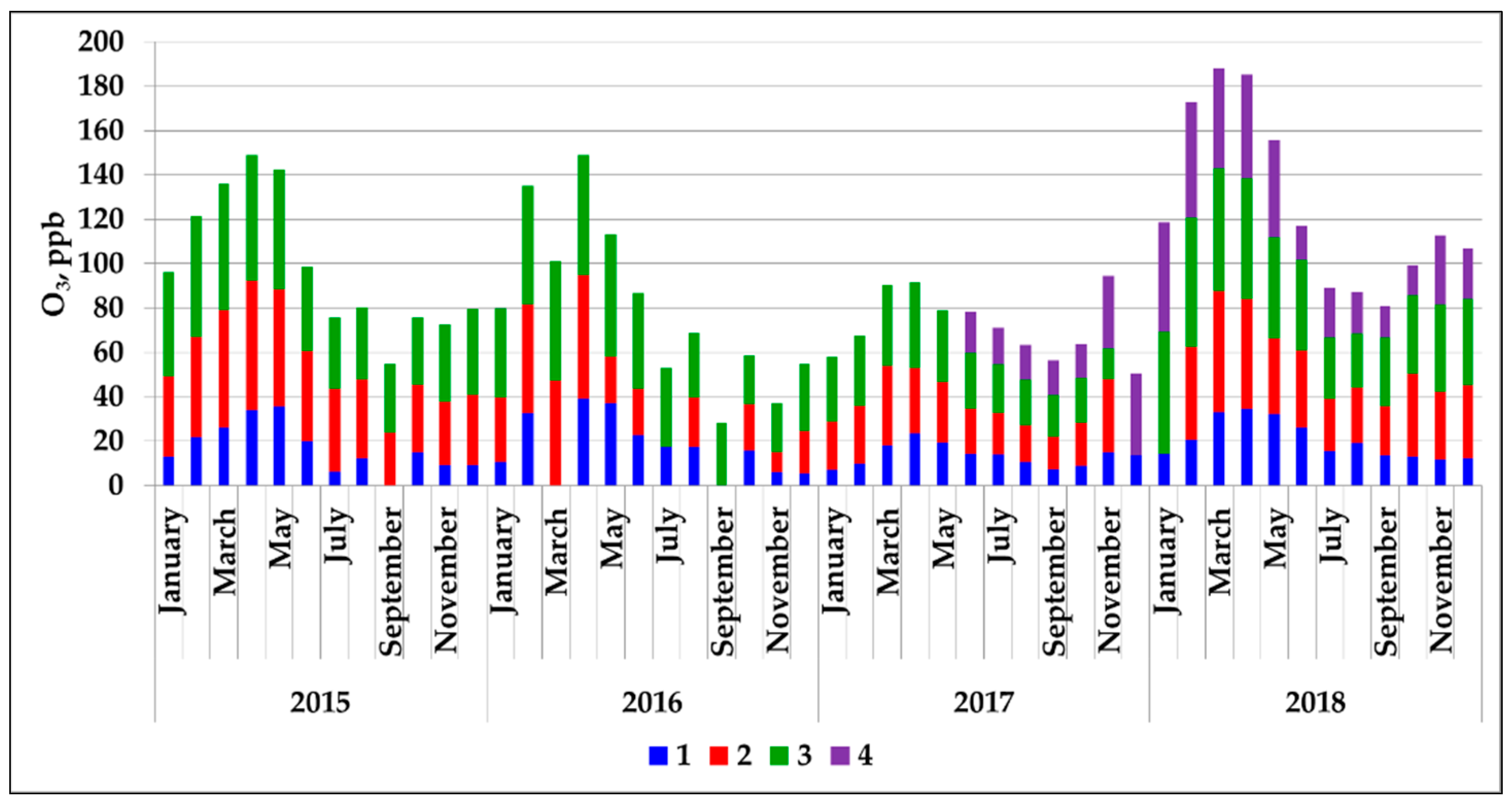
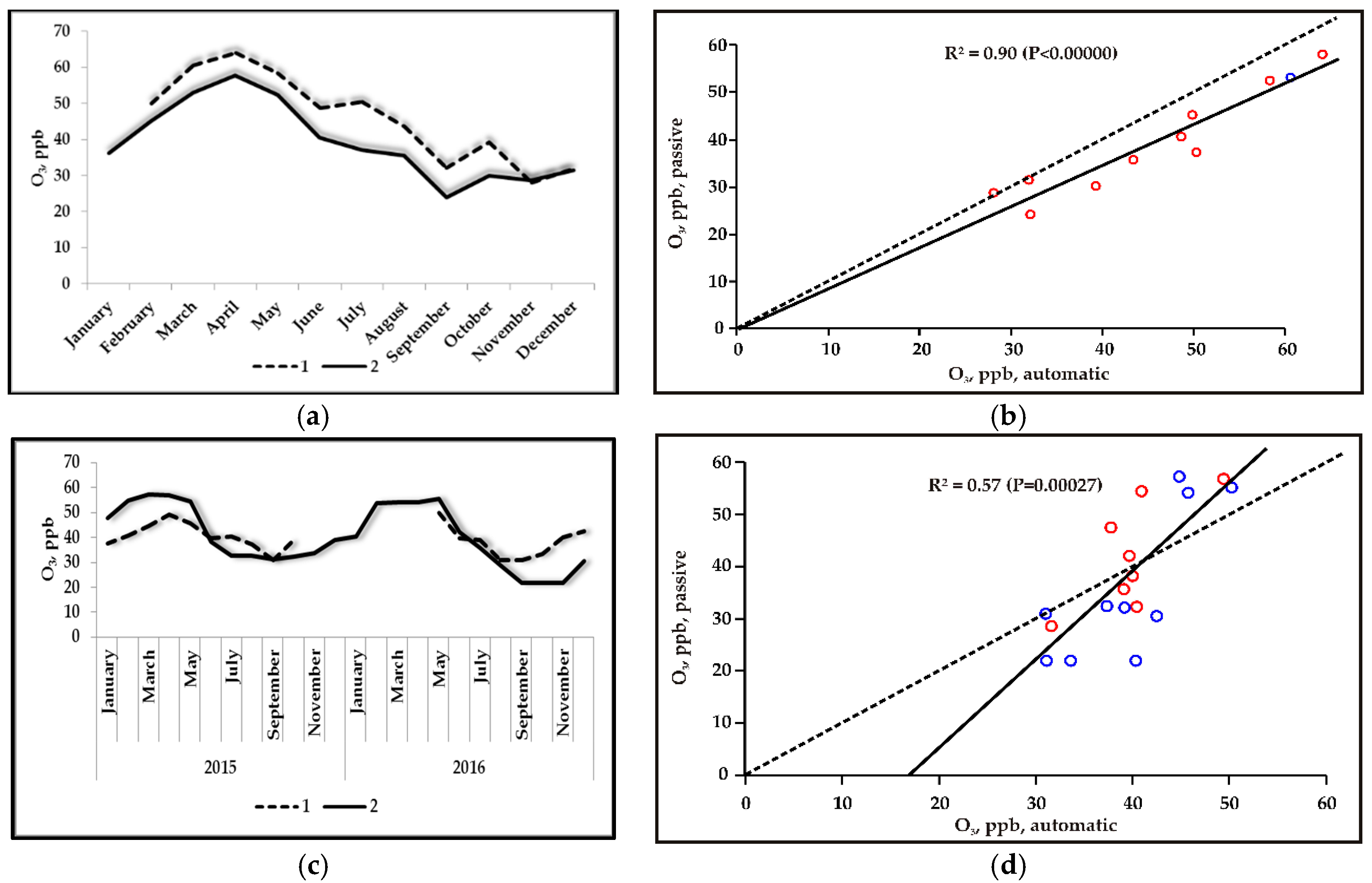
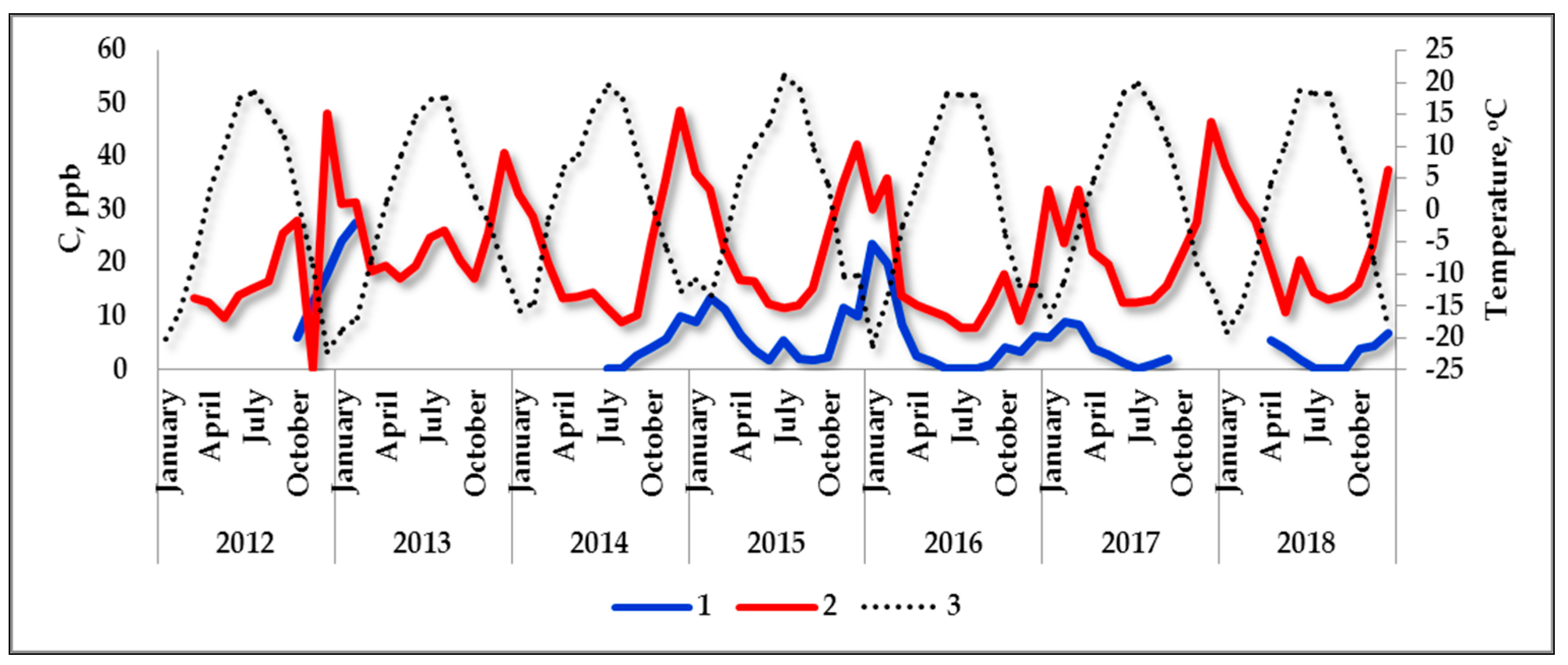
3.1. Measurement of Ozone Concentration
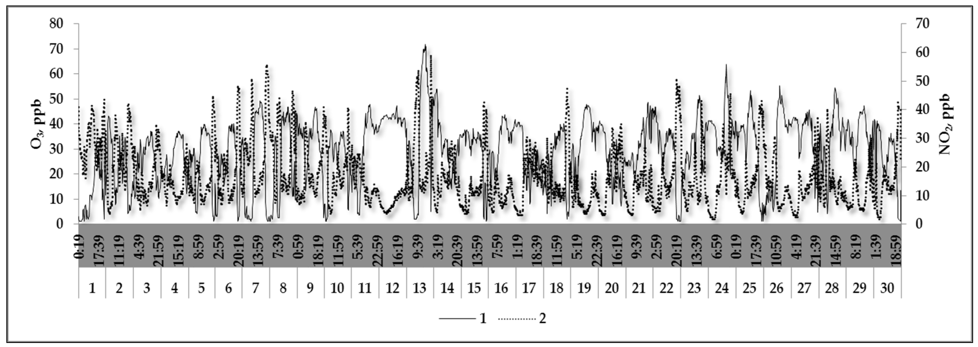
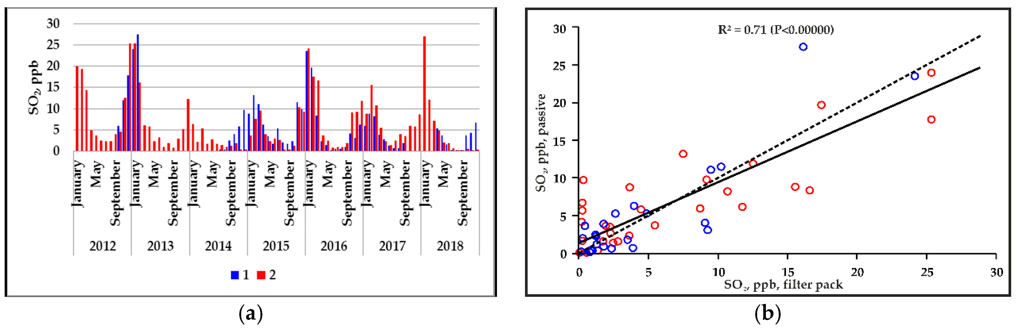
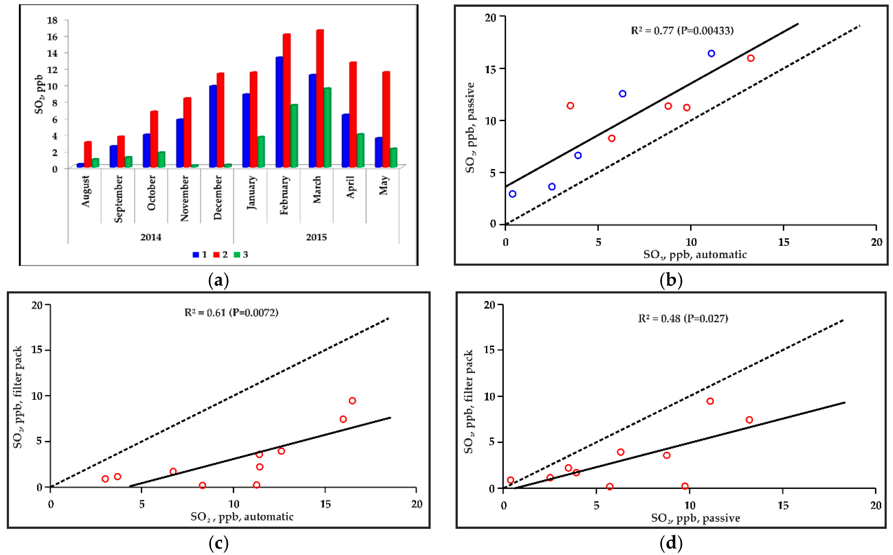
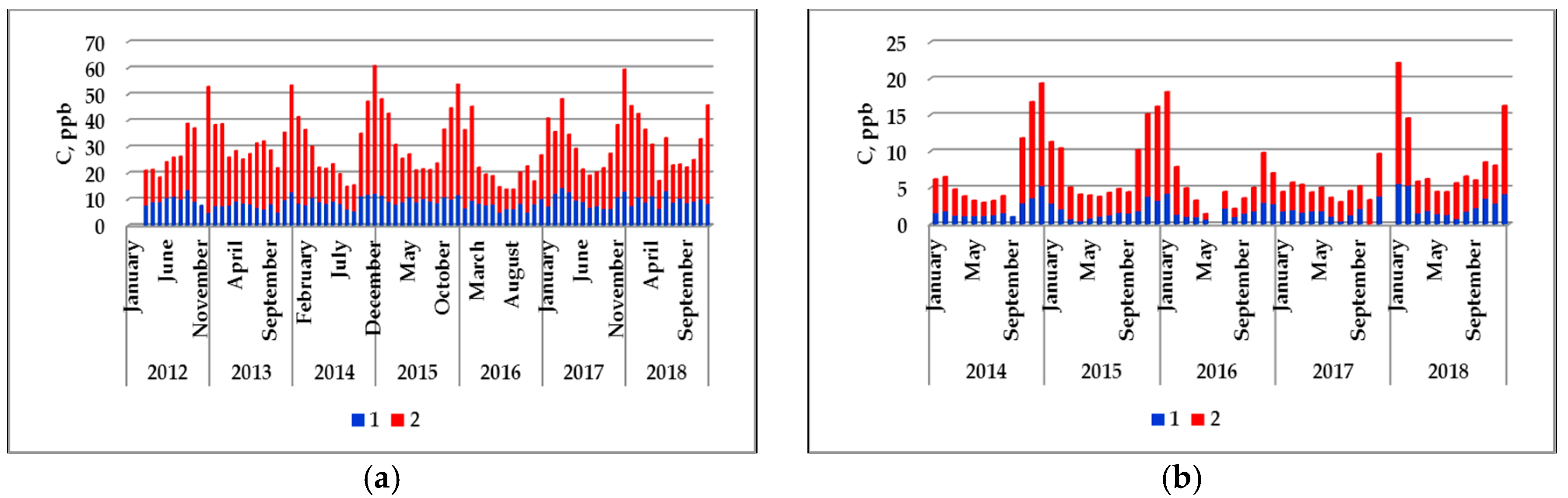
3.2. Sulfur and Nitrogen Oxides
4. Conclusions
Author Contributions
Funding
Conflicts of Interest
References
- Akimoto, H. Tropospheric Ozone a Growing Threat; Acid Deposition and Oxidant Research Center: Niigata, Japan, 2006; p. 26. [Google Scholar]
- Vingarzan, R. A review of surface ozone background levels and trends. Atmos. Environ. 2004, 38, 3431–3442. [Google Scholar] [CrossRef]
- Akimoto, H.; Narita, H. Distribution of SO2, NOx and CO2 emissions from fuel combustion and industry activities in Asia with 1° × 1° resolution. Atmos. Environ. 1994, 28, 213–225. [Google Scholar] [CrossRef]
- Rovinsky, F.Y.; Egorov, V.I. Ozone, Oxides of Nitrogen and Sulfur in The Lower Atmosphere; Hydrometeoizdat: Leningrad, Russia, 1986; 183p. (In Russian) [Google Scholar]
- Lefohn, A.S.; Malley, C.S.; Simon, H.; Wells, B.; Xu, X.; Zhang, L.; Wang, T. Responses of human health and vegetation exposure metrics to changes in ozone concentration distributions in the European Union, United States, and China. Atmos. Environ. 2017, 152, 123–145. [Google Scholar] [CrossRef]
- EANET (Acid Deposition Monitoring Network in East Asia). Available online: https://www.eanet.asia (accessed on 10 July 2019).
- Karagulian, F.; Belis, C.A.; Dora, C.F.C.; Pruss-Ustun, A.M.; Bonjour, S.; Adair-Rohani, H.; Amann, M. Contributions to cities’ ambient particulate matter (PM): A systematic review of local source contributions at global level. Atmos. Environ. 2015, 120, 475–483. [Google Scholar] [CrossRef]
- Pochanart, P.; Kato, S.; Katsuno, T.; Akimoto, H. Eurasian continental background and regionally polluted levels of ozone and CO observed in northeast Asia. Atmos. Environ. 2004, 38, 1325–1336. [Google Scholar] [CrossRef]
- Sahu, S.K.; Beig, G.; Parkhi, N. Critical Emissions from the Largest On-Road Transport Network in South Asia. Aerosol Air Qual. Res. 2014, 1, 135–144. [Google Scholar] [CrossRef]
- Brief Statistical Handbook. Irkutsk Region. 2016. Available online: http://irkutskstat.gks.ru/wps/wcm/connect/rosstat_ts/irkutskstat/ru/publications/official_publications/electronic_versions/archive/ (accessed on 15 August 2019).
- Guerranti, C.; Benetti, F.; Cucciniello, R.; Damiani, D.; Perra, G.; Proto, A.; Rossi, F.; Marchettini, N. Pollutants monitoring and air quality evaluation in a confined environment: The ‘Majesty’ of Ambrogio Lorenzetti in the St. Augustine Church in Siena (Italy). Atmos. Pollut. Res. 2016, 7, 754–761. [Google Scholar] [CrossRef]
- Alejo, D.; Morales, M.C.; Nunez, V.; Bencsd, L.; Grieken, R.V.; Espen, P.V. Monitoring of tropospheric ozone in the ambient air with passive samplers. Microchem. J. 2011, 99, 383–387. [Google Scholar] [CrossRef]
- Pekey, B.; Ozaslan, U. Spatial distribution of SO2, NO2, and O3 concentrations in an industrial city of Turkey using a passive sampling method. Clean Soil Air Water 2013, 41, 423–428. [Google Scholar] [CrossRef]
- Vardoulakis, S.; Lumbreras, J.; Solazzo, E. Comparative evaluation of nitrogen oxides and ozone passive diffusion tubes for exposure studies. Atmos. Environ. 2009, 43, 2509–2517. [Google Scholar] [CrossRef]
- Brown, R.H. Monitoring the ambient environment with diffusive samplers: Theory and practical considerations. J. Environ. Monit. 2000, 2, 1–9. [Google Scholar] [CrossRef] [PubMed]
- Kot-Wasik, A.; Zabiegała, B.; Urbanowicz, M.; Dominiak, E.; Wasik, A.; Namiesnik, J. Advances in passive sampling in environmental studies. Anal. Chim. Acta 2007, 602, 141–163. [Google Scholar] [CrossRef] [PubMed]
- Kholyavitskaya, A.A.; Potemkin, V.L.; Golobokova, L.P.; Khodzher, T.V. Testing of the passive method for measuring ozone concentrations in the atmospheric surface layer (Mondy station, East Siberia). Atmos. Ocean. Opt. 2011, 24, 828–831. (In Russian) [Google Scholar]
- Khuriganova, O.; Obolkin, V.; Akimoto, H.; Ohizumi, T.; Khodzher, T.; Potemkin, V.; Golobokova, L. Long-term dynamics of ozone in surface atmosphere at remote mountain, rural and urban sites of South-East Siberia, Russia. Open Access Libr. J. 2016, 3, e2578. [Google Scholar] [CrossRef]
- Obolkin, V.A.; Potemkin, V.L.; Makukhin, V.L.; Khodzher, T.V.; Chipanina, E.V. Far transfer of trails, ejected by regional electric power stations to the South Baikal water area. Atmos. Ocean. Opt. 2017, 30, 60–65. [Google Scholar] [CrossRef]
- Protocol for Ozone Measurement Using the Ozone Passive Sampler Badge. Available online: http://ogawausa.com/wp-content/uploads/2019/02/proozone_01_2019.pdf (accessed on 25 June 2019).
- NO, NO2, NOx, and SO2 Sampling Protocol Using the Ogawa Sampler; Ogawa & Co.: Pompano Beach, FL, USA, 1998; Available online: http://ogawausa.com/wp-content/uploads/2017/11/prono-noxno2so206_206_1117.pdf (accessed on 25 June 2019).
- Assembly of Ogawa Sampler. Available online: http://ogawausa.com/wp-content/uploads/2014/04/assembly.pdf (accessed on 7 June 2019).
- EANET (Acid Deposition Monitoring Network in East Asia). Technical Manual for Dry Deposition Flux Estimation in East Asia. 2010. Available online: https://www.eanet.asia/wp-content/uploads/2019/04/techdoc_fp.pdf (accessed on 15 August 2019).
- EANET (Acid Deposition Monitoring Network in East Asia). Technical Document for Filter pack Method in East Asia. 2003. Available online: https://www.eanet.asia/wp-content/uploads/2019/04/techdry.pdf (accessed on 15 August 2019).
- EANET (Acid Deposition Monitoring Network in East Asia). Inter-Laboratory Comparison Project Report 2017. 2019. Available online: https://monitoring.eanet.asia/document/public/index (accessed on 7 June 2019).
- WMO (World Meteorological Organization). Study 60 Summary. 2019. Lab 700115 Russia. Available online: http://qasac-americas.org/study-results (accessed on 28 May 2019).
- EMEP (European Monitoring and Evaluation Programme). EMEP Laboratory Intercomparison. Results: EMEP 36. 2018. Available online: https://projects.nilu.no//ccc/intercomparison/index.html (accessed on 28 May 2019).
- Fox, J.; Friendly, M.; Weisberg, S. Hypothesis tests for multivariate linear models using the car package. R J. 2013, 5, 39–52. [Google Scholar] [CrossRef]
- Masiol, M.; Squizzato, S.; Chalupa, D.; Rich, D.Q.; Hopke, P.K. Evaluation and field calibration of a low-cost ozone monitor at a regulatory urban monitoring station. Aerosol Air Qual. Res. 2018, 18, 2029–2037. [Google Scholar] [CrossRef]
- Pochanart, P.; Akimoto, H.; Khodzher, T.; Kajii, Y.; Potemkin, V. Regional background ozone and carbon monoxide variations in remote Siberia (East Asia). J. Geophys. Res. 2003, 108, 4028. [Google Scholar] [CrossRef]
- Wang, T.; Xue, L.; Brimblecombe, P.; Lam, Y.F.; Li, L.; Zhang, L. Ozone pollution in China: A review of concentrations, meteorological influences, chemical precursors and effects. Sci. Total Environ. 2017, 575, 1582–1596. [Google Scholar] [CrossRef]
- Moiseenko, K.B.; Shtabkin, Y.A.; Berezina, E.V.; Skorokhod, A.I. Regional photochemical surface ozone sources in Europe and Western Siberia. Izvestiya Atmos. Ocean. Phys. 2018, 54, 545–557. [Google Scholar] [CrossRef]
- Pitari, G.; Iachetti, D.; Genova, G.D.; Luca, N.D.; Sovde, O.A.; Hodnebrog, O.; Lee, D.S.; Lim, L.L. Impact of coupled NOx/aerosol aircraft emissions on ozone photochemistry and radiative forcing. Atmosphere 2015, 6, 751–782. [Google Scholar] [CrossRef]
- Tan, Z.; Lu, K.; Jiang, M.; Su, R.; Dong, H.; Zeng, L.; Xie, S.; Tan, Q.; Zhang, Y. Exploring ozone pollution in Chengdu, southwestern China: A case study from radical chemistry to O3-VOC-NOx sensitivity. Sci. Total Environ. 2018, 636, 775–786. [Google Scholar] [CrossRef] [PubMed]
- Belan, B.D. Ozone in Troposphere; Institute of Atmosphere Optics, SB RAS: Tomsk, Russia, 2010; p. 487. (In Russian) [Google Scholar]
- Jenkin, M.E.; Clemitshaw, K.C. Ozone and other secondary photochemical pollutants: Chemical processes governing their formation in the planetary boundary layer. Atmos. Environ. 2000, 34, 2499–2527. [Google Scholar] [CrossRef]
- Badamassi, A.; Xu, D.; Leyla, B.H. The impact of residential combustion emissions on health expenditures: Empirical evidence from Sub-Saharan Africa. Atmosphere 2017, 8, 157. [Google Scholar] [CrossRef]
- Marinaite, I.I.; Molozhnikova, E.V.; Khodzher, T.V. PAHs transfer and intake to the water area of Lake Baikal during the summer forest fires in 2016. In Proceedings of the SPIE 10833, 24th International Symposium on Atmospheric and Ocean Optics: Atmospheric Physics, Tomsk, USSR, 2–5 July 2018; Volume 1083374. [Google Scholar] [CrossRef]
- Shvidenko, A.Z.; Shchepanenko, D.G. Climate change and wildfires in Russia. Russ. J. Forest Sci. (Lesovedenie) 2013, 5, 50–61. (In Russia) [Google Scholar] [CrossRef]
- Zhu, Q.; Liu, Y.; Jia, R.; Hua, S.; Shao, T.; Wang, B. A numerical simulation study on the impact of smoke aerosols from Russian forest fires on the air pollution over Asia. Atmos. Environ. 2018, 182, 263–274. [Google Scholar] [CrossRef]
- Ehlers, C.; Klemp, D.; Rohrer, F.; Mihelcic, D.; Wegener, R.; Kiendler-Scharr, A.; Wahner, A. Twenty years of ambient observations of nitrogen oxides and specified hydrocarbons in air masses dominated by traffic emissions in Germany. Faraday Discuss. 2016, 189, 407–437. [Google Scholar] [CrossRef]
- Kiros, F.; Shakya, K.M.; Rupakheti, M.; Regmi, R.P.; Maharjan, R.; Byanju, R.M.; Naja, M.; Mahata, K.; Kathayat, B.; Peltier, R.E. Variability of anthropogenic gases: nitrogen oxides, sulfur dioxide, ozone and ammonia in Kathmandu Valley, Nepal. Aerosol Air Qual. Res. 2017, 18, 602–622. [Google Scholar] [CrossRef]
- Zhang, L.; Lee, C.S.; Zhang, R.; Chen, L. Spatial and temporal evaluation of longterm trend (2005–2014) of OMI retrieved NO2 and SO2 concentrations in Henan Province, China. Atmos. Environ. 2017, 154, 151–166. [Google Scholar] [CrossRef]
- He, J.; Xu, H.; Balasubramanian, R.; Chan, Y.C.; Wang, C. Comparison of NO2 and SO2 measurements using different passive samplers in tropical environment. Aerosol Air Qual. Res. 2014, 14, 355–363. [Google Scholar] [CrossRef]
- Mottaa, O.; Cucciniellob, R.; Feminab, R.; Pirontib, C.; Protob, A. Development of a new radial passive sampling device for atmospheric NOx determination. Talanta 2018, 190, 199–203. [Google Scholar] [CrossRef] [PubMed]


| Gases | Absorption Reagent (a Volume Concentration) | Analyte; Analytical Method |
|---|---|---|
| SO2 | 10% triethanolamine | SO42−; Ion chromatography |
| O3 | Nitrite ion NaNO2 + K2CO3 | NO3−; Ion chromatography |
| NO2 | 10% triethanolamine | NO2−; Ion chromatography |
| NOx | 10% triethanolamine + PTIO (2-phenyl-1-4,4,5,5-tetramethylimidazoline-3-oxide-1-oxyl) | NO2−; Ion chromatography |
| Gases | Formulas |
|---|---|
| SO2 (ppb) = αSO2 × WSO2/t | αSO2 = 39.4 × (293/(273 + T))1.83 |
| NO (ppb) = αNO × (WNOx − WNO2)/t | αNO = 45.3 × (−0.046 × T + 219.94)/(−0.439 × P × RH + 208.16) |
| NO2 (ppb) = αNO2 × WNO2/t | αNO2 = 77.2 × (2.003 × T + 89.41)/(0.637 × P × RH + 131.47) |
| O3 (ppb) = αO3 × WO3/t | αO3 = 46.2 × 102 × (293/(273 + T))1.83/(9.94 × ln (t) − 6.53) |
© 2019 by the authors. Licensee MDPI, Basel, Switzerland. This article is an open access article distributed under the terms and conditions of the Creative Commons Attribution (CC BY) license (http://creativecommons.org/licenses/by/4.0/).
Share and Cite
Khuriganova, O.I.; Obolkin, V.A.; Golobokova, L.P.; Bukin, Y.S.; Khodzher, T.V. Passive Sampling as a Low-Cost Method for Monitoring Air Pollutants in the Baikal Region (Eastern Siberia). Atmosphere 2019, 10, 470. https://0-doi-org.brum.beds.ac.uk/10.3390/atmos10080470
Khuriganova OI, Obolkin VA, Golobokova LP, Bukin YS, Khodzher TV. Passive Sampling as a Low-Cost Method for Monitoring Air Pollutants in the Baikal Region (Eastern Siberia). Atmosphere. 2019; 10(8):470. https://0-doi-org.brum.beds.ac.uk/10.3390/atmos10080470
Chicago/Turabian StyleKhuriganova, Olga I., Vladimir A. Obolkin, Liudmila P. Golobokova, Yuri S. Bukin, and Tamara V. Khodzher. 2019. "Passive Sampling as a Low-Cost Method for Monitoring Air Pollutants in the Baikal Region (Eastern Siberia)" Atmosphere 10, no. 8: 470. https://0-doi-org.brum.beds.ac.uk/10.3390/atmos10080470