Article

Surface Heat Fluxes over the Northern Arabian Gulf and the Northern Red Sea: Evaluation of ECMWF-ERA5 and NASA-MERRA2 Reanalyses

1
Marine Science Department, College of Science, Kuwait University, Safat 13060, Kuwait
2
Department of Oceanography, Texas A&M University, College Station, TX 77843, USA
3
Physical Oceanography Department, Woods Hole Oceanographic Institution, Woods Hole, MA 02543, USA
*
Author to whom correspondence should be addressed.
Atmosphere 2019, 10(9), 504; https://doi.org/10.3390/atmos10090504
Submission received: 16 July 2019 / Revised: 14 August 2019 / Accepted: 21 August 2019 / Published: 28 August 2019
(This article belongs to the Section Biosphere/Hydrosphere/Land–Atmosphere Interactions)

Abstract

:
The air–sea heat fluxes in marginal seas and under extreme weather conditions constitute an essential source for energy transport and mixing dynamics. To reproduce these effects in numerical models, we need a better understanding of these fluxes. In response to this demand, we undertook a study to examine the surface heat fluxes in the Arabian Gulf (2013 to 2014) and Red Sea (2008 to 2010)—the two salty Indian Ocean marginal seas. We use high-quality buoy observations from offshore meteorological stations and data from two reanalysis products, the Modern-Era Retrospective analysis for Research and Applications version 2 (MERRA2) from the National Aeronautics and Space Administration (NASA) and ERA5, the fifth generation of the European Centre for Medium-Range Weather Forecasts (ECMWF) atmospheric reanalyses of global climate. Comparison of the reanalyses with the in situ-derived fluxes shows that both products underestimate the net heat fluxes in the Gulf and the Red Sea, with biases up to −45 W/m 2 in MERRA2. The reanalyses reproduce relatively well the seasonal variability in the two regions and the effects of wind events on air–sea fluxes. The results suggest that when forcing numerical models, ERA5 might provide a preferable dataset of surface heat fluxes for the Arabian Gulf while for the Red Sea the MERRA2 seems preferable.

1. Introduction

Understanding the variability of air–sea heat fluxes is key in determining changes in weather systems (e.g., the work by the authors of [1]), climatic conditions (e.g., the work by the authors of [2]), sea surface temperature (SST) (e.g., the work by the authors of [3]), and the transfer of gases across the air–sea interface (e.g., the work by the authors of [4]).
Despite the significance of air–sea heat fluxes in ocean–atmosphere dynamics, there is presently a gap in our knowledge regarding these fluxes in marginal seas such as the Arabian/Persian Gulf (hereafter the Gulf) and the Red Sea (Figure 1A). A major reason for this is the historical scarcity and accuracy of in situ observations in these regions. These two marginal seas are characterized by unique surface heat losses of up to 671 W/m 2 due to dry wind events that produce dust storms (13–20 annually [5,6]) which significantly lower the atmospheric transparency and may partly or fully block solar radiation [7,8,9]. An example of these wind events is the locally known as ‘Shamal’ in the Gulf [6,10,11] and westward winds over the northern Red Sea. The Shamal winds are encountered throughout the year, with the highest frequency during summer [12] and their occurrence in winter appears to be closely related to dry air outbreaks due to mountain gap westward winds in the Red Sea [13,14]. Furthermore, extreme evaporation rates of up to 5 m/yr [8,15,16] and dust emissions of up to 94 Mt driven by such events play a major role in the transport of moisture and dust to central Asia, Africa, and the Arabian Peninsula [14,17].
Intense surface heat losses produced by wind events often drive convective conditions which provide the forcing for intensive convective mixing processes observed in oceans (e.g., works by the authors of [18,19]). As a result of the extreme heat loss conditions deep water masses are formed in both the northern Gulf and the northern Red Sea (e.g., works by [20,21,22], and references therein). These waters masses are the Gulf Deep Water (GDW) and the Red Sea Overflow Water (RSOW) and are major contributors to the large-scale circulation of the Indian Ocean (IO) (e.g., works by the authors of [23]).
If we are to accurately simulate the present as well as future scenarios of extreme weather events and climate change, both locally and on basin scales—there are indications that the northwest IO is becoming saltier as a result of changes in the GDW and RSOW characteristics (e.g., works by the authors of [24,25])—a better understanding of the air–sea fluxes in the Gulf and the Red Sea is essential.
Simulating the response of the ocean to climate variability requires time series of surface heat fluxes over long time periods and large spatial scales. Reanalysis data from numerical weather products offers these requirements. Compared to other data sources (e.g., ship-, buoy-, and satellite-based) reanalysis data has the advantage of combining excellent spatial and temporal coverage. However, such products do require ground-truth data for validation in a variety of regions as they might be susceptible to systematic biases and random errors (e.g., works by the authors of [27,28]). The main aim of the present work, is to understand such biases and errors in both the Gulf and the Red Sea as previously conducted by Kubota et al. [29] in the Kurshio region, Japan and by Weller et al. [30] in the Arabian Sea. Our study focuses on evaluating air–sea fluxes from reanalysis products in comparison to offshore, in situ-derived fluxes, with the objective of finding which of the reanalysis products would constitute the best choice for forcing atmospheric and oceanic numerical models in these regions.
Currently, the few available air–sea flux studies of the Gulf and Red Sea have used ships, buoys, coastal platforms, or oceanographic instruments that are sparsely distributed, and thus result in significant uncertainties in the heat flux estimates. For instance, studies have used the International Comprehensive Ocean–Atmosphere DataSet (ICOADS [31]) heat fluxes to force numerical models such as Hybrid Coordinate Ocean Model (HYCOM [32]) and the Coupled Hydrodynamical Ecological Model for Regional and Shelf Seas (COHERENS [33]) to simulate the Gulf surface and subsurface circulation [34,35,36].
A study by Johns et al. [37] used global air–sea heat fluxes generated by the Southampton Oceanography Center (SOC), an improved version of ICOADS, to examine the heat budgets of the Gulf. Using the SOC improved version, reduced the error in the monthly heat flux from 60 W/m 2 to 4 W/m 2 by applying corrections to longwave and shortwave radiation, imposed by strong aerosol loading measured by the Advanced Very High Resolution Radiometer (AVHRR) [38,39]. Similar uncertainties in the air–sea fluxes were also observed for the Red Sea. For example, SOC overestimates the mean in situ heat fluxes by ~60 W/m 2 [20], whereas ICOADS overestimates the heat flux by 100 W/m 2 [40].
In another study by Thoppil and Hogan [8], which examined the Gulf’s response to winter wind events, they included a section comparing the basin-averaged monthly Objectively Analyzed air–sea Heat Fluxes (OAFlux; satellite-based) [41] to those from HYCOM for 2004. The study concluded that an annual discrepancy of −2.3 W/m 2 existed between the two products and that the discrepancy was especially high during summer, when HYCOM estimated a heat flux larger by 34 W/m 2 than OAFlux.
The few available studies in the Gulf and Red Sea referenced above all lack comparisons to observations, making the results presented here unique as well as essential for improvement of the accuracy of the regional numerical ocean models.
This paper is structured as follows. In Section 2, we describe the buoy observations and reanalysis data sources and the statistical approach used for the comparison. Section 3 and Section 4 describe the results and discuss the comparison between the observations and the reanalysis products with a focus on the unique Gulf seasonal wind events. These sections also discuss the annual trends, and the diurnal and seasonal cycles of the air–sea heat fluxes in the Gulf and Red Sea. Summary and conclusions are given in Section 5.

2. Datasets and Methods

2.1. Gulf Observations

The Gulf is a 990-km-long semi-enclosed sea located between latitudes 24 ° and 30 ° N, with an average depth of 36 m [42]. General circulation in the Gulf is similar to those in other marginal seas, such as the Red Sea and Mediterranean Sea, and is driven by wind, thermohaline flows and water exchange (annual 1–2 × 10 5 m 3 /s) through the Strait of Hormuz with the Arabian Sea to the south [21]. The circulation in the northern part of the Gulf (location of the study region, see Figure 1) is driven by the dominant northwesterly winds, which force a general southerly flow, and the river discharge (average 703 m 3 /s [43]) from the Shatt-al-Arab at the northern limit [44]. The descending dry air in this region produces arid desert conditions. The northern part of the Gulf is characterized by extreme summer air temperatures (up to 51 ° C) and near-zero winter temperatures [6].
For the Gulf, we used two in situ data sets between January 2013 and March 2014. The first dataset is from the Kuwait Meteorological Office (KMO) buoy near the Sea Island Terminal. This buoy, located at 29.11 ° N, 48.30 ° E, is approximately 15 km offshore (Figure 1C). The measurements include hourly air temperature measured by a sensor mounted in a passive radiation shield at a nominal distance of 2 m above sea level (ASL), sea surface temperature at 2 m depth, wind speed and direction at 5 m ASL, relative humidity at 2 m ASL, barometric pressure at 2 m ASL, and downward shortwave and longwave radiation at 3 m ASL.
The second data source is from a meteorological station mounted on a pole at a nominal distance of 7 m ASL on a pier on Qarooh Island. The island is roughly circular in shape, with a diameter of 250 m, and is located 40 km off the mainland and 120 km south of the Shatt-al-Arab river mouth (Figure 1C). The dataset consists of measurements every 5 min of wind speed and direction, air temperature and humidity, incoming shortwave radiation, incoming longwave radiation, barometric pressure, and rain. SST measurements were obtained at 3.5 min intervals at a depth of 0.1 m, from a water temperature logger mounted inside a small surface float.
The two observational datasets will be presented separately in the results section to gain spatial information and to evaluate the ability of the reanalysis data to reproduce spatial variability from stations that are 15 and 40 km offshore. We linearly interpolated the nearest four sea based reanalysis grid points to match those of the observations locations (Figure 1C), similar to the method used by Kubota et al. [29].

2.2. Red Sea Observations

Similar to the Gulf, the Red Sea is a semi-enclosed marginal sea of the northwest IO, characterized by an arid climate, extreme salinity and water temperature. It extends for more than 2000 km between the latitudes of 12 ° N to 30 ° N, where it bifurcates into the Gulf of Suez (west) and Gulf of Aqaba (east) at the extreme north (Figure 1A) [45]. At the south, the Red Sea communicates through the shallow and narrow (~20 km) Strait of Bab-al-Mandab with the Gulf of Aden and the Arabian Sea [20,45,46,47,48]. Different from the Gulf, the river runoff in the Red Sea is negligible, and the Red Sea is much deeper with a mean depth of 524 m and maximum of almost 3000 m [45].
Surface winds in the Red Sea are mostly along the central axis, constrained by the mountains on both sides of the basin, and regulated by the Indian monsoonal regime (e.g., the work by the authors of [13]). In the northern part (north of 19 ° N), the winds are more stable and predominantly southeastward all year-round. In the southern region, the winds reverse direction seasonally due to the monsoons. Because of the that, in the summer monsoon (June-September), the winds are unidirectional over the entire Red Sea. In the winter monsoon (October-May), the winds in the northern and southern parts blow in the opposite direction and form a convergence zone (RSCZ) with light winds near 19 ° N, as recently studied by Menezes et al. [13]. North of the RSCZ, synoptic conditions in winter usually disrupt the along-axis winds giving rise to across-axis (westward) surface wind events [13,49]. These westward winds originate in the Arabian Desert and reach the Red Sea through the gaps in the coastal mountain range. Menezes et al. [14] show that these dry air outbreaks sharply increase the Red Sea evaporation (latent heat flux) in winter, and may be related to the occurrence of winter Shamal winds in the Gulf. In summer, near the RSCZ, the Red Sea also experience the sharp Tokar Gap wind jets that blow from Sudan towards Saudi Arabia [49].
In the literature, traditionally, the Red Sea is thought to be composed of three sub-regions, the southern, the central and the northern. However, in the present work, we adopt the convention of Menezes et al. [13] and Menezes et al. [14] and use the RSCZ mean position (19 ° N) as dividing the Red Sea into just two subregions: the northern and the southern Red Sea.
Between October 2008 and December 2010, the Woods Hole Oceanographic Institution (WHOI) in collaboration with the King Abdullah University of Science and Technology (KAUST) maintained a surface buoy in the northern Red Sea (22.17 ° N; 38.50 ° E) to study air–sea interaction, the primary driver of the basin-scale Red Sea circulation (Figure 1B) [20,46,50]. This buoy is the only in situ observation of air–sea flux related variables in the entire Red Sea, and several works have analyzed its data (e.g., works by the authors of [13,14,20,49,50]). The buoy was located 55 km offshore of Thuwal, anchored at a water depth of 693 m, and measured both meteorological and oceanic parameters. Over the two years, there were two one-year-long mooring deployments, with a gap of approximately two days for the buoy replacement. The following parameters were measured; temperature, salinity, and ocean currents from the sea surface to the bottom; wind velocity and direction; air temperature; humidity; barometric pressure; incoming shortwave (incident sunlight) and longwave (infrared) radiation; precipitation; and surface waves. The atmospheric instrument component of the buoy consisted of two Improved Meteorological (IMET) systems, with most parameters being measured once per minute [50].
For comparison with the observation-derived surface air–sea fluxes, we select the corresponding ERA5 and MERRA2 data from the nearest grid point to the WHOI/KAUST mooring position. In ERA5, the center of the chosen grid point is at 22.06 ° N and 38.53 ° E, ~12.6 km from the buoy site. In MERRA2, the center of the closest grid point is ~32 km from the mooring site at 22.00 ° N and 38.75 ° E (Figure 1B).

2.3. Estimation of Air–Sea Heat Fluxes

Using the hourly-averaged in situ measurements described above, we estimated the net heat flux, Q n e t , using the Coupled Ocean–Atmosphere Response Experiment (COARE 3.0) formulation [51], as the sum of the four heat components:
Q n e t = Q s w + Q l w + Q L + Q S ,
where Q s w is the net shortwave radiation corrected for albedo, Q l w is the difference between the directly measured downward longwave radiation and the calculated surface-emitted radiation, Q L and Q S are the latent and sensible heat fluxes, respectively, estimated from the wind speed, humidity, and temperature such that
Q L = ρ a i r C e L e U z ( q s q z ) , a n d
Q S = ρ a i r C h C p U z ( T s ( T z + γ z ) ) ,
where ρ a i r is the air density, L e is latent heat vaporization, C p the specific heat of air at constant pressure, and subscripts z and s denote their surface and air values at a reference height, respectively. U z is the scalar wind speed with the inclusion of convective gustiness, T z is the air temperature corrected for the adiabatic laps rate, γ z , q z is the specific humidity of air converted from the relative humidity observations, and q s is the 98% of the saturation specific humidity of air at the sea surface temperature, T s , to account for salinity [52].
The Q L and Q S are related to the meteorological parameters (wind, temperature, and humidity) by the moisture, C e , and heat exchange C h , coefficients, respectively. These exchange coefficients depend on atmospheric stability and surface roughness length:
C e = κ l n ( z z u ) ψ u ( z L ) κ l n ( z z h ) ψ q ( z L ) , and
C h = κ l n ( z z u ) ψ u ( z L ) κ l n ( z z T ) ψ T ( z L ) ,
where κ is the von Karman constant; ψ u , ψ q , and ψ T are empirical functions describing atmospheric boundary layer that are dependent on the ratio of z and the Monin–Obukhov length scale, L; and z u , z h , and z T are the surface roughness lengths that characterize the neutral transfer of the surface for momentum, humidity, and heat, respectively [53].
The COARE 3.0 includes an option to apply a correction for solar heating and evaporative cooling of the skin that was deemed necessary due to the strong solar radiation and evaporation in the study region. However, the option of wind current speed correction was not used for the Gulf due to the absence of near-surface currents at all stations, although used for the WHOI/KAUST Red Sea buoy.
The COARE formulation is widely used by ocean and lake observationalist and modelers (e.g., works by the authors of [54,55]) as well as air–sea interaction scientists (e.g., works by the authors of [29,56]), and is presently considered the state-of-the-art method to estimate air–sea surface heat fluxes [57]. Despite the widely use of COARE 3.0 (over 1730 cites to date), its ability is limited to wind speeds of <20 m/s, where its coefficient exchange uncertainty increases with increasing wind speed from 5% for winds 0–10 m/s to 10% for winds 10–20 m/s [51]. This uncertainty is mainly a result of the disruption of the near surface sub-layer by wave breaking and sea spray generated by the high winds [58].
In addition, using the present method to compare estimates from offshore observations of air–sea heat fluxes to those from reanalysis products has been shown to be suitable in several studies (e.g., works by the authors of [59,60]). This study is therefore important as it does highlight the possible differences in forcing fluxes when use is made of reanalysis surface fluxes at times when observational data might be unavailable.
The two most widely used reanalysis products are the ECMWF-ERA Interim and NASA-MERRA [61]. In this study we have used the most recent versions of these two reanalysis products to compare Q s w , Q l w , Q L , Q S , wind, air temperature, humidity, and SST to the Gulf and Red Sea buoy observations.
The first is the 5th generation (ERA5) and most recent reanalysis product from ECMWF. ERA5 is an improved version of, and replacement to, ERA Interim [62] and features a new numerical weather product (IFS Cycle 41r2). This updated version was produced using 12-h 4D-Var data assimilation and a larger amount of assimilated data than before. Compared to the ERA Interim, ERA5 generates higher resolution data on a 31 km grid at hourly intervals from 1979 to the present. Moreover, numerous reprocessed datasets and recent instruments that could not be implemented in the ERA Interim dataset were available to provide improved forecasts [63].
ERA5 produces daily short (18 h) forecasts for all parameters that are initialized twice at 06:00 and 18:00 UTC in 18 steps (1 step/hr). For example, for time 06:00, step 6 will be at 12:00 UTC. In this study, to obtain hourly data, only steps 1 to 12 were selected, thus providing hourly data from 06:00 to 18:00 (12 steps) and from 18:00 to 06:00 (12 steps). The values of the four heat fluxes in units of W/m 2 s were an accumulation of the hourly steps. The daily means of the four heat fluxes were computed by aggregating all hourly steps from 00:00 to 23:59 UTC then dividing by 86,400 s (24 h) to provide a mean value centered at 12:00 UTC. Other parameters were provided as hourly means that were then averaged over 24 h to obtain a daily mean centered at 12:00 UTC.
The second product evaluated in this study is MERRA2, which was developed by NASA. Unlike MERRA1, the MERRA2 uses an upgraded version of the Goddard Earth Observing System Model, Version 5 (GEOS-5 [64]) that includes aerosol analysis [65]. This upgraded data system has the ability to incorporate information from newer microwave sounders and hyperspectral infrared radiance instruments, as well as other datasets, and provides improved analysis schemes. Similar to MERRA1, this updated version was produced using 6-h 3D-Var data assimilation to provide hourly analysis fields from 1980 to the present at a spatial resolution of ∼50 km (0.625 ° × 0.5 ° ) [66].
MERRA2 produces hourly forecasts that are initialized at 00:00, 06:00, 12:00, and 18:00 UTC. All studied parameters were averaged over 24 h to obtain a daily mean centered at 12:00 UTC.
To assess and contrast the accuracy of the ERA5 and MERRA2 reanalysis products, we compared hourly averaged air–sea parameters collected from two offshore stations to those from the two reanalysis products using the following statistics; mean bias error ( M B E ), root mean square error ( R M S E ), and the commonly used Pearson correlation coefficient (r), which quantifies the linear relation of two independent variables (e.g., the work by the authors of [67]). We used a p-value of 0.05 to denote statistical significance computed using the bootstrap method (correlations are significant for p-values < 0.05) [68].
In addition, a statistical summary of these quantitative comparisons is provided in a Taylor Diagram [69]. This statistical approach has shown to be effective when comparing in situ measurements with reanalysis air–sea fluxes (e.g., works by the authors of [70,71]).

3. Results of the Heat Fluxes in the Gulf

3.1. Seasonal Cycle

The strong, seasonal swings of meteorological conditions and seasonal wind events play a major role in determining the air–sea heat fluxes leading to the formation of the Gulf Deep Water (GDW), which eventually spill into the Arabian Sea [21], and the regional advective and diffusive processes. These fluxes need to be well understood and accurately reproduced by reanalysis products in order to allow accurate forcing of numerical models used to simulate the circulation in the Gulf. We analyze next the seasonal variability of heat fluxes, followed by a detailed analysis of the various seasonal wind events and their effect on the heat fluxes. A comparison to the reanalysis products evaluates their ability to reproduce these events.

3.1.1. Observed Seasonal Heat Flux Variability

The daily mean net heat flux follows a predominantly seasonal pattern (Figure 2A,B) with a maximum heating of 249 W/m 2 occurring in June and a maximum cooling of 758 W/m 2 occurring in bursts associated with the passage of tropical storms (details in Section 3.1.2) during the autumn transition period (October) (for details of regional climate characteristics see the work by the authors of [6]).
Figure 2C,D shows the monthly net heat flux, the results of which clearly reflect seasonal changes in solar radiation output (Figure 3A,B). A net heat gain of up to 145 W/m 2 may be noted between February and August and a net cooling of up to 245 W/m 2 between September and January. The net heat flux sharply declined during the autumn period (October) compared to that of the following winter month of November (Figure 2C,D). The sharp autumn decline is mainly a result of unstable weather activity producing tropical storms, which we discuss in detail next (Section 3.1.2). From the heat flux observations investigated above, it is clear that seasonal wind events play a major role in causing abrupt changes altering the overall seasonal pattern as observed during autumn.
In comparison, a previous study by Rezaei-Latifi and Hosseinibalam [16] estimated a maximum heat flux gain of 89 W/m 2 and a maximum heat loss of 133 W/m 2 derived from NOAA’s monthly Gulf basin average net heat flux estimates between 1948 and 2009. The discrepancy between the two studies is most likely due to a tendency of the northern part of the Gulf to exhibit above-average net heat flux ranges, due to its shallow depth [16]. Further comparisons between the studies show an agreement in the sharp decline of the net heat flux during autumn (October) compared to that of the following winter months (Figure 2C,D).

3.1.2. Autumn Tropical Storms

The autumn transition period produced three main tropical storm (TS) events, on 28 September 2013 (TS 1) and 9 (TS 2) and 23 (TS 3) October 2013. The maximum daily average wind speed recorded during the study period was up to 14.3 m/s (Figure 4A,B) reducing air humidity from 76% to 39% (Figure 4C,D). The combination of stronger winds and drier air produced latent heat losses of up to 743 W/m 2 in a single day (Figure 5A,B), with latent heat loss during these events accounting for 81% of the net heat flux loss (Table 1D). Moreover, the daily average air temperature decreased by an average of 3.2 ° C for the three events (Figure 6A,B), leading to an average air–sea temperature difference of 2.5 ° C (Figure 6C,D). This lowered the sensible heat flux to only 2% (Table 1D) of the net heat flux loss. The cooling events during these three tropical storms (TS 1–3) led to the sharp decline in October’s monthly averaged heat flux to 195 W/m 2 (Figure 2C,D). The ratios of cooling by the three heat flux components (longwave radiation and latent and sensible heat fluxes) were consistent during the three tropical storms (Table 1A–C). Hence, this apparent signature associated with the tropical storm may allow the identification of such tropical storms and separate them from other wind events (details in Section 3.2).
We next analyzed the spatiotemporal patterns of two locations separately during the strongest recorded wind event TS 2 in order to evaluate the reanalysis ability to reproduce the observed spatial variability of the data from the stations at 15 and 40 km offshore. Our results (Figure 7A–D) show significant cooling starting at 153 W/m 2 pre-storm up to a daily maximum heat loss of 758 W/m 2 as winds strengthened in speed from 5.49 m/s pre-storm to 14.26 m/s. Comparison to the reanalysis products shows significant over heating simulated by ERA5 but not by MERRA2 near coast (Figure 7D). This overheating by ERA5 extends 31 km offshore and introduces a 85 (20%), a 124 (19%), and a 56 W/m 2 (21%) larger heat flux compared to the observed at the Sea Island buoy during TS 1, TS 2, and TS 3, respectively (Figure 2A). In contrast, MERRA2 provides a better agreement with the observations at the Sea Island buoy, with an average discrepancy of 19 W/m 2 (10%) during the three tropical storms combined. Both reanalysis products produce better net heat flux simulations at Qarooh Island compared to those at Sea Island with an average bias of 1% by MERRA2 and 15% by ERA5 for the three events. These better simulations are mainly driven by the absence of coastal effects at Qarooh Island compared to the Sea Island.
Combining the reanalysis errors in net heat fluxes during the three tropical storms at both study locations results in average biases of 4% produced by MERRA2 and 18% produced by ERA5. Unfortunately, despite their apparent impact on sea surface cooling there are no studies that analyze these regional tropical storms; thus, we are unable to compare our findings to those of other studies.

3.1.3. Winter Shamal Events

Unlike the unstable autumn period, the winter season is influenced by the Siberian high-pressure system [72], which stabilizes the regional climate but is commonly interrupted by cold frontal systems that progress from the northwest [73]. These frontal systems are commonly followed by the well known ‘winter Shamals’ and occur, on average, for a total of 12 days between December and March each year [10]. Following the definition of a Shamal event (a NW-N wind with an hourly speed of ≥9.85 m/s blowing for at least 3 hr/day and for at least two consecutive days) by Al Senafi and Anis [6], a total of seven winter Shamals were observed during the study period. In the present study, we analyze the three Shamal events with the strongest winds in each month for temporal variability: 17 December 2013 (Sh 1), 8 January 2014 (Sh 2), and 7 February 2014 (Sh 3).
A detailed 40-year regional study of winter Shamals by Al Senafi and Anis [6] concluded that these events result in and increase in wind speed of up to 23 m/s, an abrupt decrease in air temperature of up to 8 ° C, and a decrease in humidity of up to 40%. These results are similar to our observations reported here of an increase in wind speed of up to 12 m/s (Figure 4A,B), an average drop in air temperature during each day of 6 ° C (Figure 6A,B), and a reduction in relative humidity of 22% (Figure 4C,D).
We next analyzed the variability of heat fluxes in response to the meteorological conditions associated with Sh 1. This event led to a heat loss of 548 W/m 2 , the second highest during the observation period (Figure 2A,B), and 13% higher than the simulated maximum reported in November–December 2004 winter Shamals by Thoppil and Hogan [8]. The latter study estimated a latent heat loss of 433 W/m 2 and sensible heat loss of 104 W/m 2 during conditions when wind speeds were 16 m/s and the air temperature decreased from 26 ° C to 21 ° C. The latent heat losses in our observations were generally lower than those of Thoppil and Hogan [8], due mainly to the relatively weaker winds (by ~4 m/s) during our observations. As expected, the latent heat flux dominated the net heat loss, accounting for 58% of the loss during Sh 1 (Table 2A). The stronger Shamal winds (Figure 4A,B), combined with drier air (Figure 4C,D), resulted in latent heat losses of up to 410 W/m 2 (Figure 5A,B). Moreover, the abrupt air temperature drop of 6 ° C (Figure 6A,B) increased the air–sea temperature gradient (Figure 6C,D) thereby increasing the sensible heat loss to 130 W/m 2 (Figure 5C,D), accounting for 19% of the net heat loss during Sh 1 (Table 2A).
Comparing the two reanalysis products spatially (Figure 7I–L) shows high near coast overheating simulated by the ECMWF’s ERA5 dataset, similar to what was observed during the autumn tropical storm period (Figure 7D). This coastal effect led to a heat flux larger by 180 W/m 2 (33%) compared to that observed at the Sea Island buoy during Sh 1 (Figure 2A). A similar difference may be noted in the ERA5 simulations during Sh 2 and Sh 3, leading to biases of 33 W/m 2 (15%) and 67 W/m 2 (24%), respectively. In comparison, MERRA2 provided a better agreement with the observations at the Sea Island station, with an average bias of 5 W/m 2 (3%) during the three winter Shamals. Similar to the results obtained for the autumn tropical storm periods, the ERA5 reanalysis product provided better net heat flux simulations at Qarooh Island than those at Sea Island, with an average bias of 10% for the three events.
Combining the simulated errors in net heat flux during the three winter Shamal events at both study locations resulted in an average bias of 2% produced by MERRA and 17% produced by ERA5. These errors are consistent with those observed during the tropical storm periods.

3.1.4. Spring Storms

Similar to the conditions during the autumn transition period (Section 3.1.2), there are no well-defined weather patterns during the spring transition (April–May), and the weather is commonly unstable [6]. A total of four spring wind events, with daily average wind speeds of ≥6 m/s were recorded, which is lower than during events in the other seasons (Figure 4A–D).
In this study, we focused on the three strongest wind events, which occurred on: April 6 (SS 1), April 22 (SS 2), and May 1 (SS 3). Daily average winds, with a maximum speed of 8.1 m/s, carried drier air into the region, causing a decrease in relative humidity from 9 to 25% (Figure 4C,D). The stronger and drier winds resulted in higher latent heat losses of up to 174 W/m 2 during these three events (Figure 5A,B), accounting for 59% of the net heat loss (Table 3D). In comparison, the maximum latent heat loss during spring was about half that of the minimum latent heat loss of 364 W/m 2 (TS 3) during autumn (Figure 5A,B). This difference was mainly the result of weaker winds (max 8.1 m/s) during spring than during the autumn storms (max 14.3 m/s) (Figure 4A,B). Moreover, the latent heat flux during spring accounted for only 59% of the net heat loss (Table 3D), compared to 81% during autumn (Table 1D).
In addition, the three strongest spring wind events resulted in cooler daily average air temperatures of 2.2 ° C (Figure 6A,B). Similar to the effect during the autumn storms, the cooler conditions were not significant enough to drive high air–sea temperature gradients such as observed during the winter Shamals (Figure 6C,D), thus limiting the sensible heat losses to 4% of the total net heat flux loss (Table 3D). However, the spring events produced higher longwave radiation losses, accounting for 37% of the net heat flux (Table 3D), twice that observed during autumn (Table 1D).
The two reanalysis products are capable of accurately simulating the average fractional contributions of the three heat flux components during the three spring events (Table 3A–C). This consistency is illustrated by the relatively small average bias of 13 W/m 2 (MERRA2) and 1 W/m 2 (ERA5) at both locations during the three events. However, comparison of the the reanalysis products shows that the biases increase near the coast (Figure 7E–H). As observed in the ERA5 simulations during autumn and winter, the coastal effects (Figure 7H) leads to elevated heat fluxes of 6 W/m 2 , 20 W/m 2 , and 6 W/m 2 larger compared to the observed at the Sea Island buoy during SS 1, SS 2, and SS 3, respectively (Figure 2A).
Both ERA5 and MERRA2 showed an average positive bias of 26 W/m 2 in net heat flux at the Sea Island during the three events. MERRA2 had a smaller positive bias (19 W/m 2 ) than ERA5 (70 W/m 2 ) at Qarooh Island (Figure 2B).

3.1.5. Summer Shamals

The unique hot and dry climate of the Gulf during summer (up to 51 ° C; [74]) is mainly driven by summer Shamals, which bring dry and extremely hot air to the region between May and July [11]. Unlike winter Shamals, summer Shamals are a prominent result of the Gulf’s persistent low-level jets which may last up to 40 days and generate winds with speeds to 30 m/s [75].
In this study, we analyze the three summer Shamal events with the strongest winds during different months: 9 June (SSh 1), 25 July (SSh 2), and 22 August (SSh 3). A detailed study Al Senafi and Anis [6] outlines the major difference between the winter and summer Shamals; the summer Shamals cause an increase in the daily average air temperature of 0.8 ° C, while the winter Shamals drive an average decrease in air temperature of 1.5 ° C. Such a difference has also been observed during this study, in which we recorded an increase in daily average temperature of 0.5 ° C during the three summer events (Figure 6A,B). This has resulted in a positive air–sea temperature gradient (Figure 6C,D), leading to sensible heat gain of 21–33 W/m 2 , rather than loss during summer (Figure 5C,D).
Although the sensible heat gain contributed to a positive net heat flux during these events, it was still insufficient to cause net heating. The net heat flux average for both locations during the three events was −38 W/m 2 , indicating that summer Shamals tend to cool the sea surface. This cooling is driven mainly by the latent heat flux, contributing 72% of the net heat loss, and longwave radiation, contributing 28% of the net heat loss during the three events (Table 4D).
Despite the fact that both reanalysis products yield consistent (≤6% difference) ratios of the contributing factors to cooling (latent heat flux and longwave radiation) during the three summer events (Table 4A–C), they still resulted in relatively high net heat flux biases of >70 W/m 2 . This result was driven mainly by the high latent heat flux biases of 58 W/m 2 and 26 W/m 2 produced by MERRA2 and ERA5, respectively (Figure 5A,B). The latent heat flux biases were due to a consistent overestimation of wind speed throughout the summer (Figure 4A,B), with summer average biases of 1.56 m/s by MERRA2 and 1.23 m/s by ERA5. Furthermore, both reanalysis products consistently estimated drier air than was observed during the summer, with average biases of 23% by MERRA2 and 11% by ERA5 (Figure 4C,D). The combination of overestimating wind speed and drier conditions during the summer led to the high latent heat flux biases. Although MERRA2 showed a smaller longwave radiation bias of 1 W/m 2 compared to the 21 W/m 2 bias by ERA5 (Figure 3C,D), it still produced a higher net heat flux bias than ERA5. This was mainly because the higher latent heat flux biases that outweighed (72%) the longwave radiation contribution to the net heat flux.
Spatially, both reanalysis products captured the net cooling from the pre-SSh 1 period to the day of the event as the northwesterly winds strengthened (Figure 7M–P). However, similar to previous seasons, the ERA5 reanalysis product continued to show coastal effect causing higher net heat flux values at the Sea Island buoy than at the Qarooh Island station (Figure 7D). This coastal effect incorrectly minimized the overcooling bias of ERA5 reducing it to 31 W/m 2 at the Sea Island buoy (Figure 2A). Estimates of both reanalysis products beyond 33 km from the coast consistently overcooled in comparison to the observations, with ERA5 resulting in a larger bias of 100 W/m 2 due to the reasons explained above (Figure 7N–P).

3.2. Comparison of Wind Events

One of the challenges facing scientists is to clearly define a wind event to provide a consistent and standardized basis for identifying and comparing such events [6]. In the present study, we observed that seasonal wind events have a cooling ratio between longwave radiation, latent heat flux, and sensible heat flux that may act as a ‘finger print’, distinguishing between seasons. This fingerprint may then be used to characterize, define, and identify dominant regional seasonal wind events. Comparing the four types of wind events in this study, i.e., tropical storms, winter Shamals, spring wind events, and summer Shamals—shows that each has unique characteristics that distinguish it from the other seasons. These unique characteristics are the ratios of cooling between longwave radiation and latent and sensible heat fluxes that correspond to the different meteorological conditions associated with each event.
Winter Shamals can be distinguished by the unique sharp cooling spikes in the sensible heat loss (Figure 5C,D). These cooling spikes are not as pronounced as those in other periods, due mainly to the sharp decrease in air temperature that produces a larger difference between the air temperature and SST (Figure 6C,D). Although TS 2 produced a relatively high sensible heat loss (Figure 5C,D), it still maintained a sensible heat flux cooling ratio of only 4% (Table 1B). The unique characteristics of the winter Shamal events that were consistent throughout all the events are the ratios of cooling between longwave radiation and latent and sensible heat fluxes. All winter Shamals maintained 54–58% latent heat loss, 16–19% sensible heat loss, and 23–30% longwave radiation loss (Table 2A–C).
In comparison, autumn tropical storms maintained 78–82% latent heat loss, an almost negligible 0–4% sensible heat loss, and 14–20% longwave radiation loss (Table 1A–C). The difference between heat losses of tropical storm and winter Shamal events heat losses is mainly the relative 90% increase in the sensible heat flux that is driven by the cold air carried by winter Shamals, generating a larger air–sea temperature gradient.
Similarly, when comparing spring wind events with other events, we notice that although they maintained low sensible heat losses ≤5% (Table 3A–C), and were similar to those observed during autumn storms (Table 1A–C), they can be distinguished by the larger (≥30%) longwave radiation losses.
In contrast, summer Shamals can be distinguished by their heating spikes in the sensible and latent heat fluxes. These conditions resulted in zero cooling by the sensible heat flux due to the increase in temperature associated with this event and the high latent heat losses. This situation resulted in unique cooling ratios of 72% for latent heat flux and 28% for longwave radiation (Table 4A–D).
Using the unique cooling ratios to distinguish and identify seasonal wind events, which has not been used in previous studies, did show to be effective throughout the study period and provided consistent results for each seasonal event.

3.3. Comparison of Annual Means

Comparing observations with reanalysis products of net heat flux shows significant correlations (r ≥ 0.84, p-value < 0.05; Table 5D) for both reanalysis products at both locations throughout the study period (Figure 2A,B). This suggests that the selected reanalysis products can adequately estimate the various wind events as well as seasonal variability.
The ERA5 reanalysis product provided smaller biases at Qarooh Island, with an MBE of −2 W/m 2 , compared to −32 W/m 2 by MERRA2, indicating significant cooling by the latter (Table 5B). Estimates of ERA5 produced less biased net heat fluxes than those of SOC [37] and OAFlux Thoppil and Hogan [8], with minimum biases of 4 W/m 2 and −95 W/m 2 , respectively, for the Gulf region.
The reanalysis products net heat flux biases were primarily influenced by overestimation of both latent heat flux and shortwave radiation, despite the significant correlations with the observations (r = ≥ 0.85, p-value < 0.05; Table 5D). The reanalysis products produced a combined ( Q s w + Q L ) average MBE of 12 W/m 2 from ERA5 and 24 W/m 2 from MERRA2, and a high RMSE ranging between 20 and 72 W/m 2 (Table 5C) for the two heat flux components. The smallest biases were for the longwave radiation and sensible heat fluxes, where both reanalysis products had an MBE bias of ≤10 W/m 2 and a RMSE value of ≤25 W/m 2 . Based on these results, and supported by a significant (r = 0.9, p-value < 0.05) correlation, we conclude that ECMWF’s ERA5 reanalysis dataset appears to provide estimates that are closer to the observed heat flux (−2 W/m 2 by ERA5; −32 W/m 2 by MERRA2) and offers higher spatial resolution (31 km by ERA5; 50 km by MERRA2) than MERRA2. A statistical summary of these results are provided in Figure 8.
At the Sea Island buoy, both reanalysis products overcooled, with MBEs of −7 W/m 2 and −62 W/m 2 by ERA5 and MERRA2, respectively. Although the ERA5 had biases of −7 W/m 2 , the coastal effect which may be explained by ERA5’s spatial resolution that is distorted at nearshore locations incorrectly minimized overcooling biases of ERA5. In comparison, MERRA2 reanalysis product offered a lower spatial resolution, however it did not show the steep changes near the coast as observed in the ERA5 product.
The largest discrepancies between the reanalysis products and observations occurred during the summer months June–August (Figure 9), leading to a bias in the net heat loss of 24% and 27% at Qarooh and 15% and 27% at Sea Island by ERA5 and MERRA2, respectively. This bias is due to an 85% overestimation of the latent heat flux loss during summer by both reanalysis products at both locations, resulting from a combination of overestimating the wind speed by 26–37% and underestimating the humidity by 15–58%.
Overall, with the exception of summer, both reanalysis products are accurate in capturing closely the observed seasonal variability and progression, as well as capturing events with timescales on the order of days.

4. Results of the Heat Fluxes in the Red Sea

Overall, both ERA5 and MERRA2 reanalyses reproduce the surface air–sea heat fluxes in the northern Red Sea at the WHOI/KAUST buoy site (Figure 10) as we describe in this section. We shall start with the net heat flux.
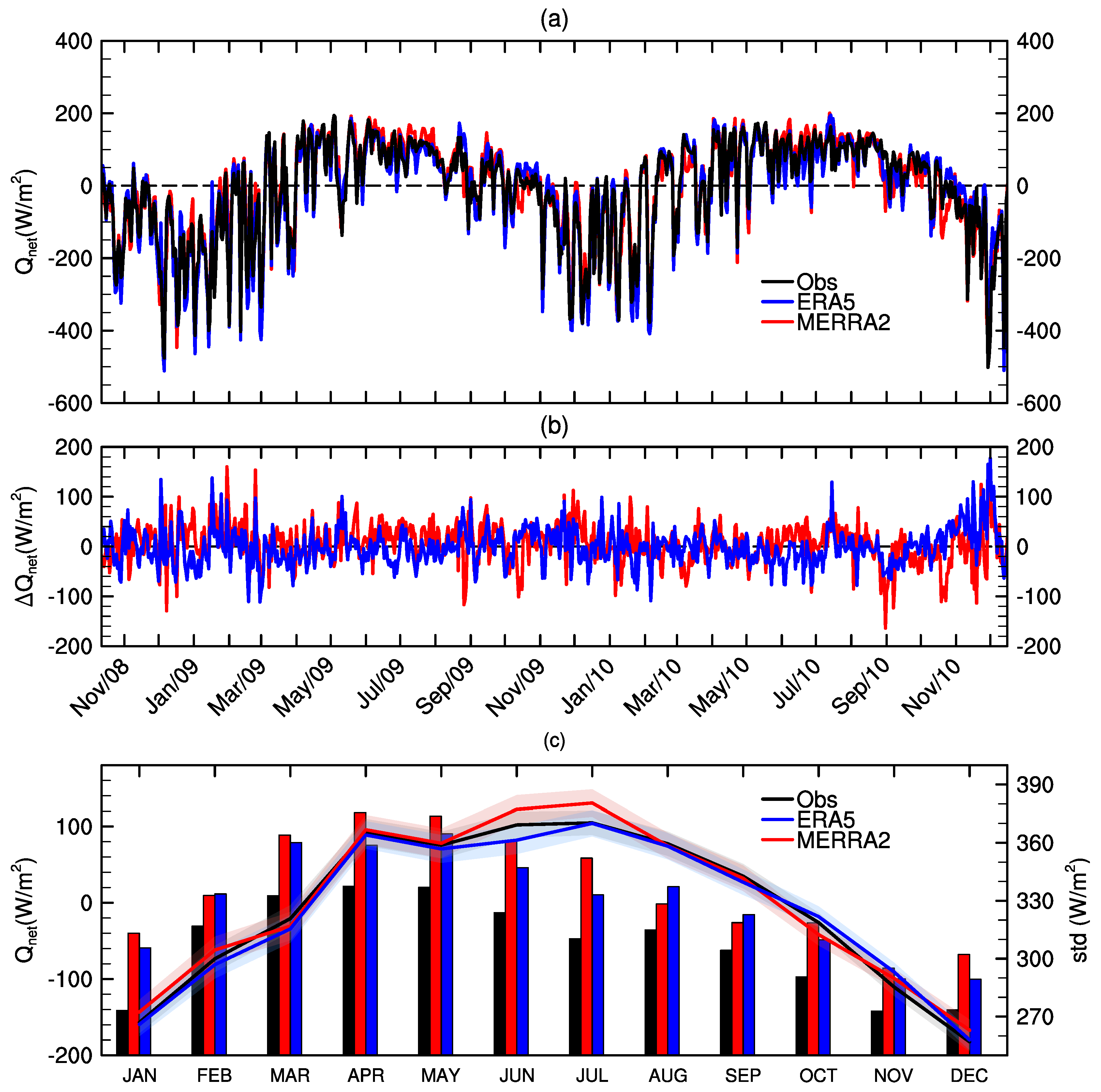
Over the two years overlapping interval (2008–2010), both MERRA2 and ERA5 show a coherent seasonality when compared with the net heat fluxes derived from in situ observations (Figure 10c). Typically, the northern Red Sea loses heat to the atmosphere ( Q n e t < 0 ) during the winter monsoon (October–March) and warms during the summer monsoon ( Q n e t > 0 ) with a peak in June–July and a secondary peak in April in both the mooring and the reanalyses data. Most of the differences between the monthly-average reanalyses and the in situ derived net heat flux occur in the summer, with MERRA2 overestimating the in situ Q n e t and ERA5 slightly underestimating it. These differences, however, are mostly inside the confidence intervals of the respective monthly means, and therefore may not be statistically significant at this level. Highest Q n e t variability occurs in the transition between the winter and the summer monsoon seasons (March–May), and lowest variability is in November–February in both observations and reanalysis data. However, Q n e t standard deviations are always higher in the reanalysis data, with MERRA2 being larger than ERA5 (Figure 10c, bars).
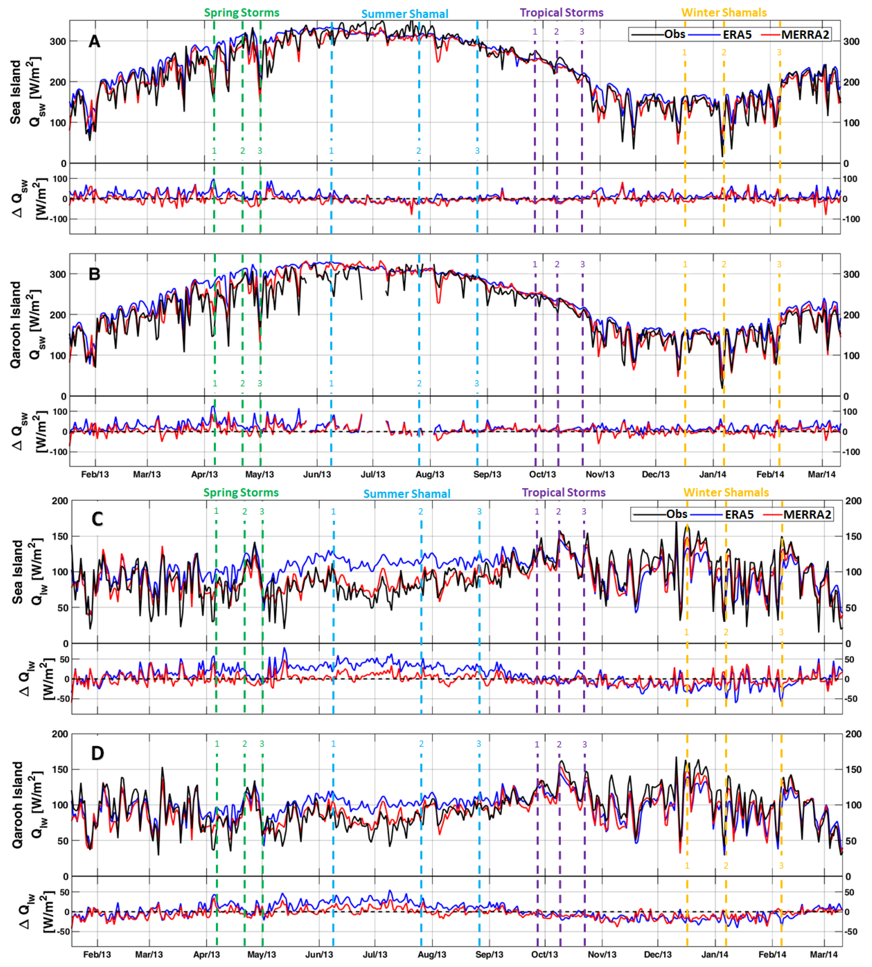
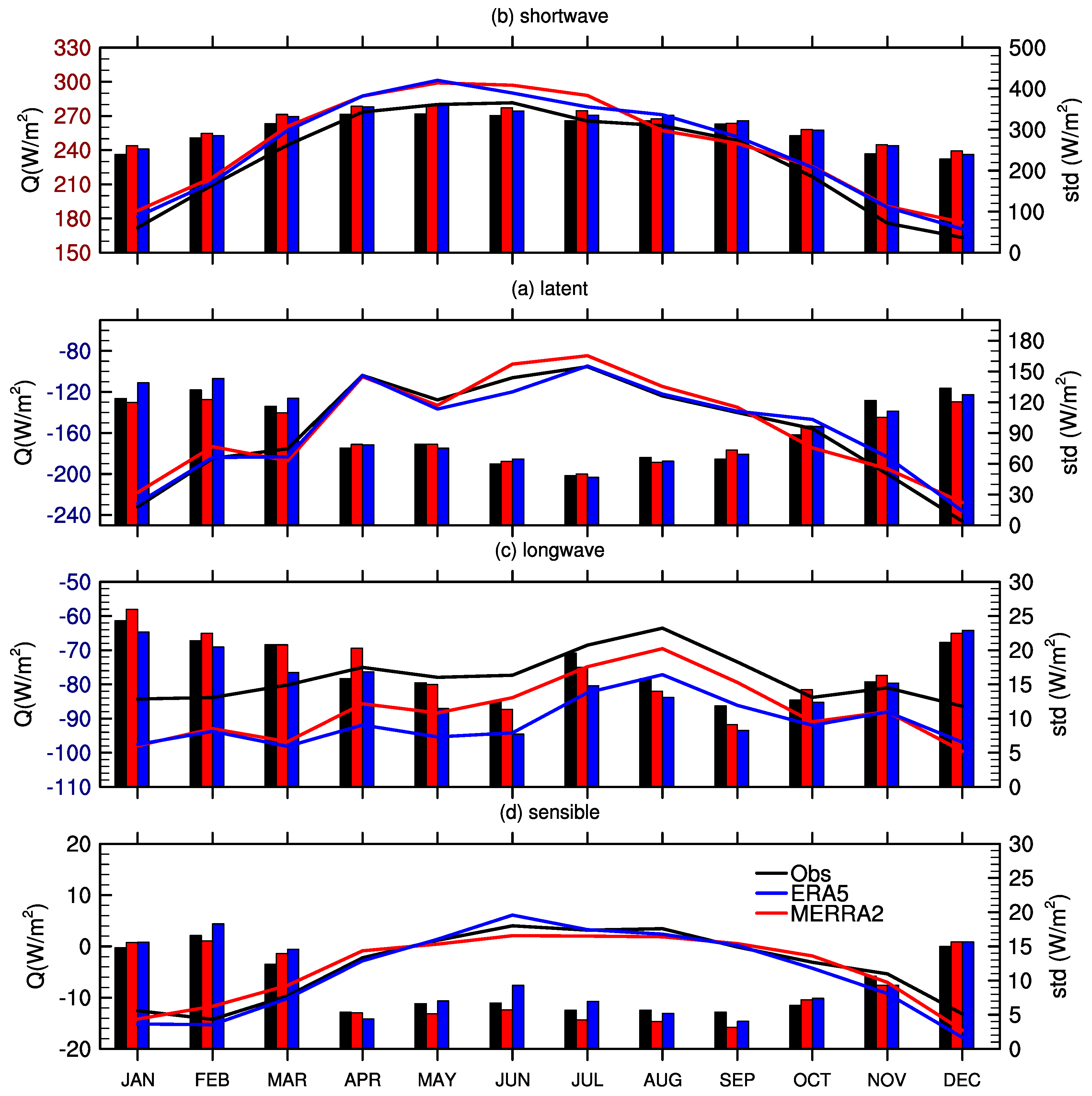
Figure 11 shows the monthly means and the respective standard deviations for each air–sea heat flux component. In both observational and reanalysis data, shortwave radiation (warming) and latent heat flux (cooling) are the primary components for the Q n e t . Longwave radiation also contributes to cooling the sea all year-round, although in a smaller degree than the latent heat flux. Shortwave radiation peaks around May–June and is slightly higher in the reanalyses, although from all components, longwave radiation shows the most substantial differences (Figure 11c). For longwave radiation, both reanalyses have a consistent cooling bias all year-round, although the bias is larger in ERA-5 than MERRA2 in summer (April–September). Sensible heat flux contributes little for Q n e t at the WHOI/KAUST buoy site.
Table 6 shows a statistical comparison between the hourly-average reanalysis data at the WHOI/KAUST buoy site, and the in situ-derived surface air–sea fluxes. For all flux components ( Q s w , Q l w , Q L , Q S , and Q n e t ), the correlations between the reanalysis data and the in situ observations are high, with linear correlation coefficients above 0.77 (all significantly different from zero at 95% confidence). The MERRA2 performance is slightly better than ERA5 at the WHOI/KAUST buoy site (higher correlations and lower R M S E ) for longwave radiation but lower for the other components. Biases, as indicated by the MBE, are much higher for the radiative fluxes (shortwave and longwave) than for the other components, with absolute values around 10 W/m 2 . For the shortwave radiation flux, the bias ( Δ = reanalysis − in situ) is positive (warmer) and for the longwave radiation is negative (cooler). Comparing the shortwave radiation fluxes at the WHOI/KAUST buoy site (in situ, ERA5, and MERRA2), we observe that the diurnal and seasonal cycles dominate the Q s w variability, and the diurnal peaks are consistently higher in the reanalyses (not shown). For instance, the mean difference between the Q s w diurnal peaks ( Δ = reanalysis − in situ) is ~30 W/m 2 for ERA5 and MERRA2, which is three times the MBE shown in Table 6.
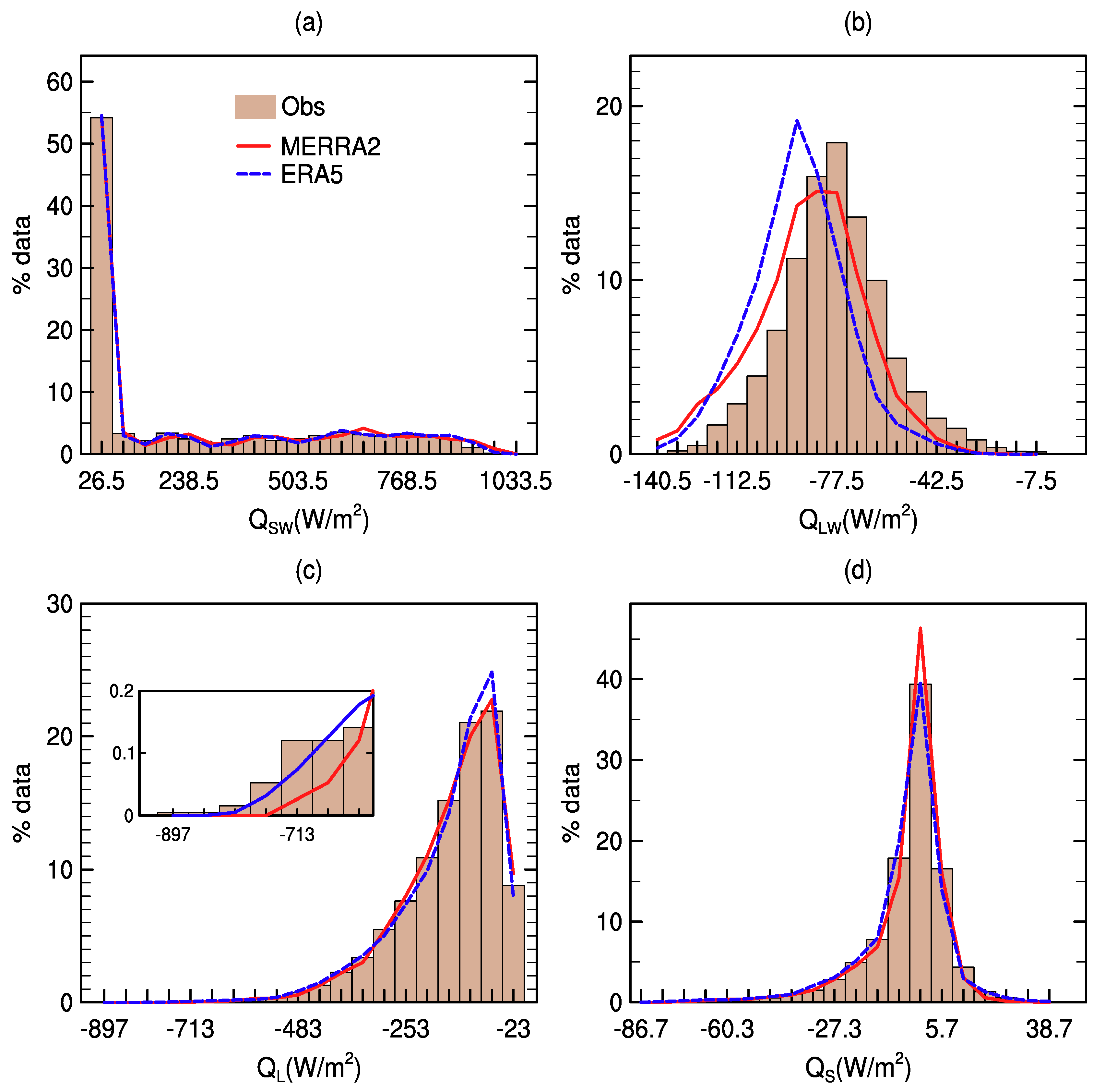
The bias in the longwave radiation flux has a different nature. The Q l w values in the reanalyses are more negative than the in situ-derived flux, i.e., enhanced sea heat loss. The Q l w cooling bias is clear in the histograms shown in Figure 12b. Both MERRA2 and ERA5 have left-shifted Q l w distributions relative to the observational histogram, with ERA5 presenting the largest displacement. The cooling bias also manifests in a lower mean, minimum and maximum Q l w values in both ERA5 and MERRA2 when compared with observations (
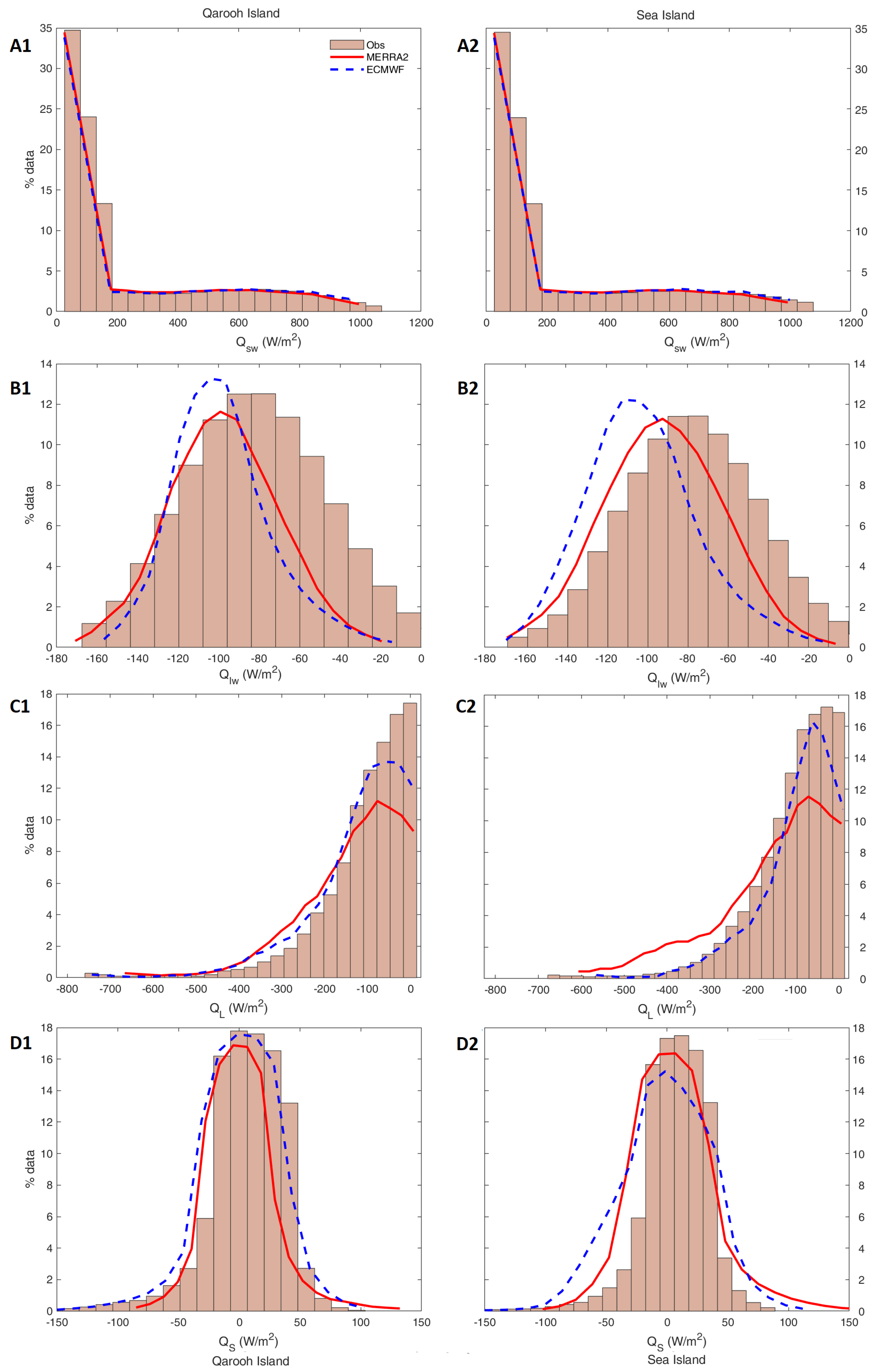
Table 6). The left-shifted distributions bias in the longwave radiation flux observed in the Red Sea histograms appear similar to those observed at both locations in the Gulf (Figure 13B). Whereas the observational distribution of Q s w , Q L , and Q S were similar to those of ERA5 and MERRA2 for both seas suggesting that reanalysis products were capable of capturing the full range (maximum to minimum) of these fluxes (Figure 12 and Figure 13).
In terms of latent heat flux, which is the primary driver of the Red Sea circulation (e.g., the work by the authors of [46]), the reanalysis capture the overall shape of the in situ distribution, but tend to underestimate extreme values (Figure 12c, inset). Menezes et al. [14] showed that ~50% of the severe heat loss days (lowest turbulent fluxes) at the WHOI/KAUST buoy observations were associated with the occurrence of westward winds that bring extreme dry air from the Arabian Desert and cause intense latent (evaporation) heat fluxes over the northern Red Sea eastern boundary. We find that both reanalysis capture these wintertime wind events (not shown). Indeed, Menezes et al. [14] have already studied extensively the impact of these westward wind events on the evaporation using MERRA2.
Between 2008 and 2010, the WHOI/KAUST buoy recorded nine events of this type (three each winter) (see, e.g., works by the authors of [13,14], for a full description of these events), and the strongest ones were recorded in December 2008 (3 to 8 December) and November 2010 (23 November to 7 December) when the in situ evaporation rates reached 6.6 and 7.1 m/yr, respectively. Table 7 shows the latent and net heat loss peaks during the six most intense events according to Menezes et al. [14]. In general, both ERA5 and MERRA2 capture the effect of such extreme events on the heat fluxes thought they underestimate the maximum latent heat loss up to 21%.
Bower and Farrar [20] compared the monthly-average air–sea heat fluxes obtained from the WHOI/KAUST mooring with the respective heat fluxes estimated from two observational products, one based on ship observations (Southampton Oceanography Center (SOC) Surface Flux Climatology) [76] and other based on satellite data (OAFlux 1 ° × 1 ° ) [41]. The results presented here indicate that ERA5 and MERRA2 perform better than the ship-based climatology reported by Bower and Farrar [20]. For example, the SOC mean Q n e t at the WHOI/KAUST buoy site shows an average heat gain of 44 W/m 2 while the in situ observations point for a heat loss of about 14 W/m 2 (Table 6, Q n e t column). Similar to the in situ data, MERRA2 also indicates a net heat loss in average at the WHOI/KAUST buoy site, although the cooling is slightly smaller than the in situ data (9 W/m 2 ). In the ERA5, on the contrary, the sea heats on average at the buoy site, but the heat gain (16 W/m 2 ) is much less than in SOC.
Most of the discrepancy between the observational-gridded products and the in situ observations described by Bower and Farrar [20] is accounted for the radiative terms, which is similar to what we found here. Bower and Farrar [20] suggest that the uncertainty in the SOC radiative fluxes at the WHOI/KAUST buoy site may arise from neglecting airborne dust effects on the regional aerosol. Atmospheric aerosols can both directly reduce the shortwave radiation reaching the sea surface by absorbing and scattering the solar incident radiation and enhance the longwave radiation by absorbing and emitting outgoing longwave radiation. In the Red Sea, Kalenderski et al. [77] showed that aerosols during wintertime dust storms reduce the solar radiance by about a quarter, affecting both longwave and shortwave radiation fluxes. A similar conclusion was found by Jish Prakash et al. [17] for the summertime. Dust activity in the Red Sea peaks in summer, particularly in July, with the northern Red Sea presenting a smaller annual cycle amplitude than the southern Red Sea (e.g., the work by the authors of [78]). In the case of the WHOI/KAUST buoy site, Jiang et al. [49] and Zhai and Bower [79] showed that in summer the region is under the influence of the Tokar gap wind jet that brings dust plumes over the northern Red Sea. In winter, dust plumes are also frequent but associated with a westward mountain gap wind jet blowing from the Arabian Desert [13,14,49]. Therefore, the uncertainty in the radiative terms might be related to the modeling of aerosols during dust storms in the reanalyses, but this conjecture needs to be further investigated and is outside the scope of the present paper.

5. Conclusions

This study examined net heat fluxes in the northern Arabian Gulf (January 2013 to March 2014) and northern Red Sea (October 2008 to December 2010) using both observations from offshore meteorological stations and reanalysis data (MERRA2 from NASA and ERA5 from ECMWF). The objective of the research was to provide guidance on which of these reanalysis datasets might be the most suitable as a surface-forcing input to numerical ocean models in the Gulf and Red Sea.
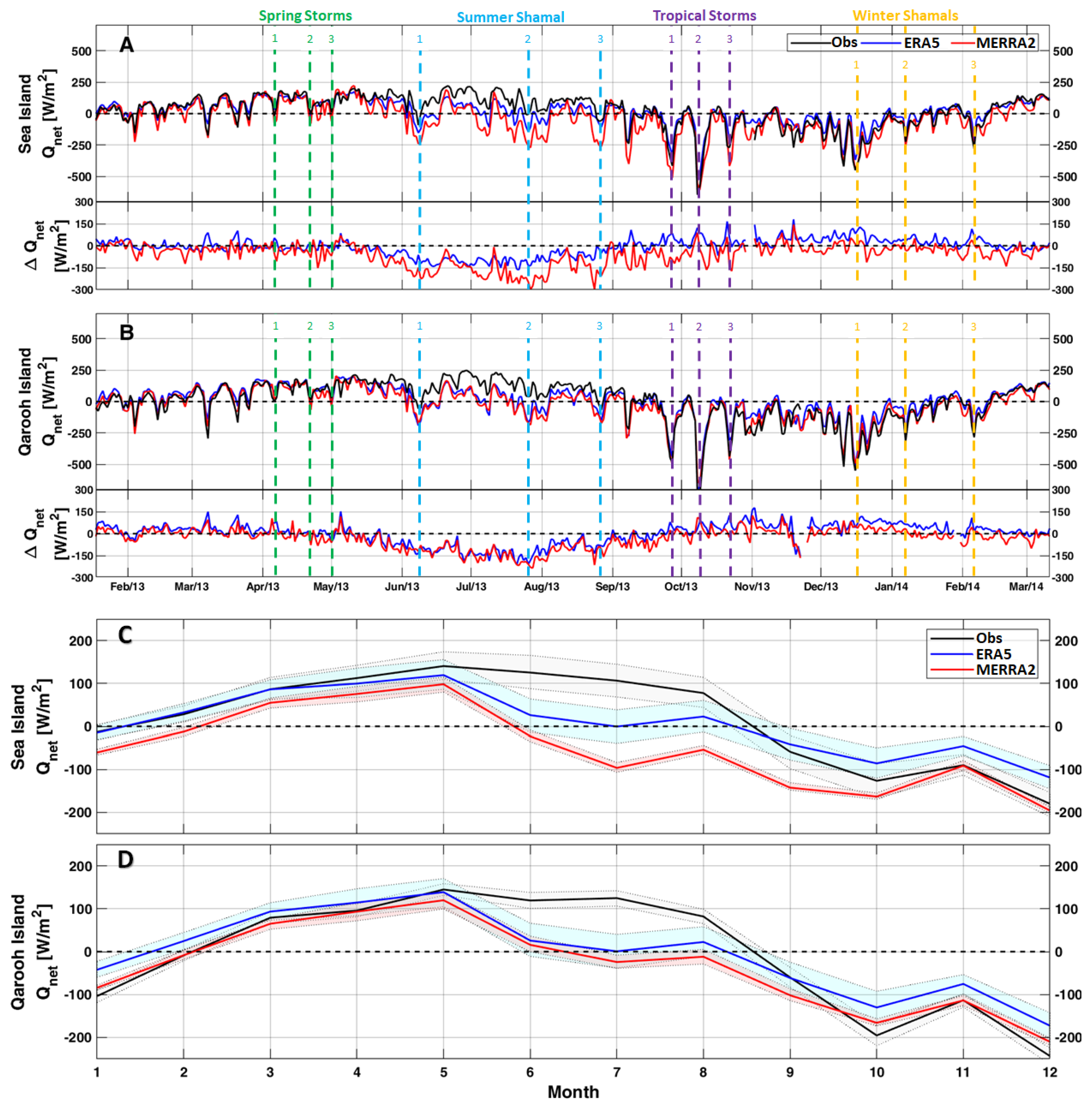
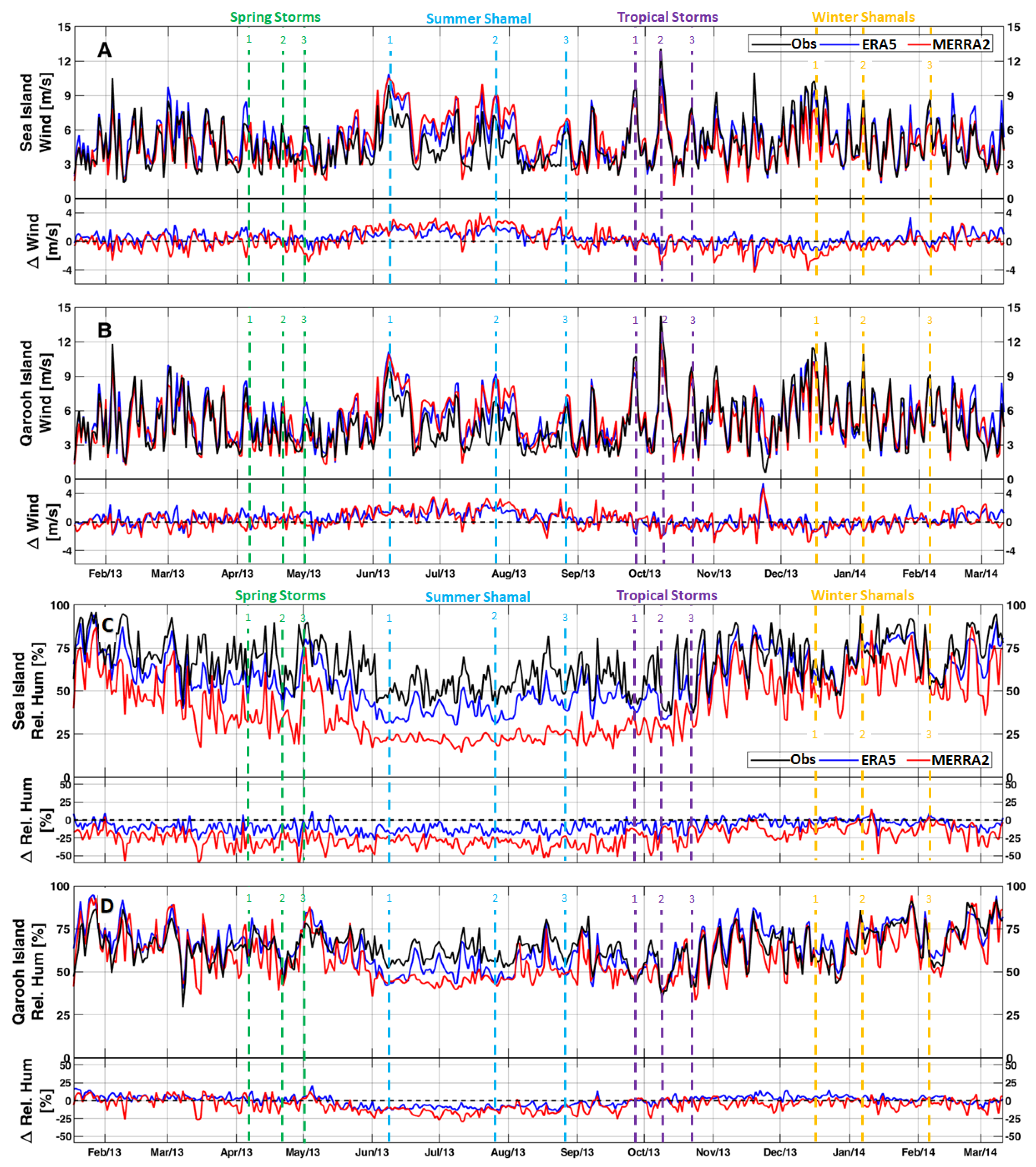
Our results for the Gulf indicate that the region experiences different wind events in each of the two main seasons (summer and winter) and the two transitional periods (spring and autumn). Detailed analysis of the wind events during the main two seasons and the transitional periods reveal that they produce unique signatures in the ratio of contributions to net cooling by longwave radiation and latent and sensible heat fluxes. As such, these signatures may provide a tool that can be used to define and identify each of these events:
  • Winter Shamals heat loss: 54–58% due to latent heat flux, 23–30% due to longwave radiation, and 16–19% due to sensible heat flux. The noticeable difference between this type of event and other events is the higher sensible heat loss due to cold air, producing higher air–sea temperature gradients.
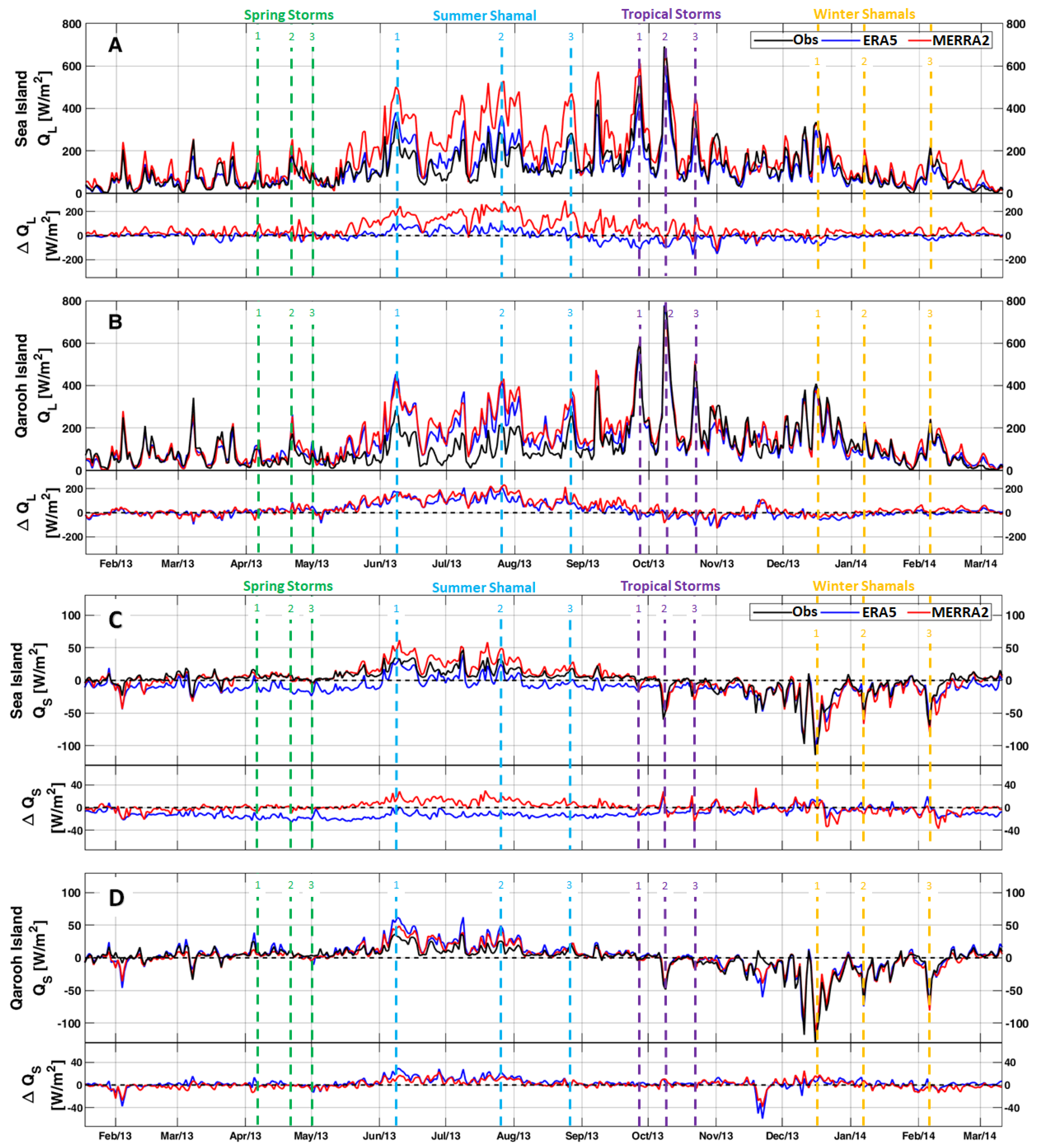
  • Summer Shamals heat loss: 71–74% due to latent heat flux, 26–29% due to longwave radiation, and ~0% due to sensible heat flux. The main difference for this event is the roughly 0% sensible heat flux loss, related to the hot air advected by summer Shamals and causing a gain in the sensible heat flux.
  • Spring wind events heat loss: 58–61% due to latent heat flux, 34–39% due to longwave radiation, and 3–5% due to sensible heat flux. The larger contribution by longwave radiation during spring wind events clearly distinguishes it from other events.
  • Autumn storms heat loss: 78–83% due to latent heat flux, 14–20% due to longwave radiation, and 0–4% due to sensible heat flux. These storms produce the strongest winds and drops in humidity, resulting in the largest latent heat flux loss ratio.
Comparison of the two reanalysis datasets in the Gulf shows that both reanalysis products underestimate the net heat flux, producing biases of −4.5 W/m 2 (ERA5) and −45 W/m 2 (MERRA2). These biases were primarily due to a combination of overestimation of the latent heat flux and shortwave radiation, resulting in a bias of 12 W/m 2 for ERA5 and 24 W/m 2 for MERRA2. The smallest bias was for longwave and sensible heat fluxes, with a value of ≤6 W/m 2 for both reanalysis products.
The comparison of the two reanalysis datasets in the Red Sea reveals that both reanalysis products produced smaller biases of −1.59 W/m 2 (ERA5) and 5.66 W/m 2 (MERRA2) compared to the Gulf. These biases were primarily due to a combination of the radiation fluxes, especially longwave radiation that presents a consistent cooling bias in both reanalysis products.
Both reanalysis products at the Gulf and Red Sea appear to not only be able to closely follow the observed seasonal variability/progression, they do well in capturing events of time scales on the order of days. Furthermore, the unique characteristics of the relative contributions of the heat flux components to cooling during the various wind events were well captured throughout the year by both reanalysis products, with biases not exceeding 5%. Although, our results show consistent and unique signatures in the ratio of contributions to net cooling for the various seasonal wind events we cannot, at this time, ascertain that these results would hold on interannual time scales. Thus, we believe that our results should provide the starting point that will encourage further studies of the relative contributions of the heat flux components as a possible tool for identifying weather events in other regions of the world ocean and as well as at longer time scales. Moreover, both reanalysis products at both regions produced the largest biases during summer, which might be related to aerosol modeling of dust storms by the reanalyses products and will need further investigation.
Based on our results, supported by the significant correlation of r = 0.90 and the smaller MBE of −4.5 W/m 2 , we conclude that ERA5 provides more accurate heat flux data than MERRA2 in the northern Gulf, while both ERA5 and MERRA2 provides accurate heat flux data in the northern Red Sea with a correlation of 0.97–0.98. Thus, we conclude that it is likely that for the regions focused on in this study that the ERA5 and MERRA2 appear, at this point, to be both suitable datasets for surface-forcing input to numerical ocean models. Furthermore, it appears that both provide an accurate picture of the seasonal variability and the effects of wind events on air–sea fluxes.

Author Contributions

The authors contributed to this paper with conceptualization, F.A.S., A.A. and V.M.; methodology, F.A.S., A.A. and V.M.; validation, F.A.S., A.A. and V.M.; formal analysis, F.A.S., A.A., and V.M.; investigation, F.A.S., A.A., and V.M.; data curation, F.A.S., A.A., and V.M.; writing—original draft preparation, F.A.S; writing—review and editing, F.A.S. and A.A.; visualization, F.A.S., A.A., and V.M.; supervision, F.A.S.; project administration, F.A.S.; funding acquisition, F.A.S. and V.M.

Funding

This study was funded by the Research Sector at Kuwait University (project #ZS03/16) and by NSF (grant #OCE-1435665) supporting V.M.

Acknowledgments

We thank the Kuwait Meteorological Office and Tom Farrar (WHOI) for providing the observational data. We also thank the Computational and Information Systems Laboratory at the National Center for Atmospheric Research, ECMWF, and NASA for providing online access to the reanalysis data. The Red Sea mooring data was collected during the WHOI-KAUST collaboration (award numbers USA00001, USA00002, and KSA00011).

Conflicts of Interest

The authors declare no conflicts of interest.

References

  1. Zhou, S.; Zhai, X.; Renfrew, I.A. The Impact of High-Frequency Weather Systems on SST and Surface Mixed Layer in the Central Arabian Sea. J. Geophys. Res. Ocean 2018, 123, 1091–1104. [Google Scholar] [CrossRef]
  2. Terray, P.; Kamala, K.; Masson, S.; Madec, G.; Sahai, A.K.; Luo, J.J.; Yamagata, T. The role of the intra-daily SST variability in the Indian monsoon variability and monsoon-ENSO-IOD relationships in a global coupled model. Clim. Dyn. 2012, 39, 729–754. [Google Scholar] [CrossRef]
  3. Shinoda, T. Impact of the diurnal cycle of solar radiation on intraseasonal SST variability in the western equatorial Pacific. J. Clim. 2005, 18, 2628–2636. [Google Scholar] [CrossRef]
  4. Blomquist, B.W.; Brumer, S.E.; Fairall, C.W.; Huebert, B.J.; Zappa, C.J.; Brooks, I.M.; Yang, M.; Bariteau, L.; Prytherch, J.; Hare, J.E.; et al. Wind Speed and Sea State Dependencies of air–sea Gas Transfer: Results From the High Wind Speed Gas Exchange Study (HiWinGS). J. Geophys. Res. Ocean 2017, 122, 8034–8062. [Google Scholar] [CrossRef]
  5. Zolina, O.; Dufour, A.; Gulev, S.K.; Stenchikov, G. Regional Hydrological Cycle over the Red Sea in ERA-Interim. J. Hydrometeorol. 2017, 18, 65–83. [Google Scholar] [CrossRef]
  6. Al Senafi, F.; Anis, A. Shamals and climate variability in the Northern Arabian/Persian Gulf from 1973 to 2012. Int. J. Climatol. 2015, 35, 4509–4528. [Google Scholar] [CrossRef]
  7. Barkan, J.; Alpert, P. The Linkage Between Solar Insolation and Dust in the Major World Deserts. Open Atmos. Sci. J. 2010, 4, 101–113. [Google Scholar] [CrossRef]
  8. Thoppil, P.; Hogan, P. Persian Gulf response to a wintertime shamal wind event. Deep Sea Res. Part I Oceanogr. Res. Pap. 2010, 57, 946–955. [Google Scholar] [CrossRef] [Green Version]
  9. Osipov, S.; Stenchikov, G. Simulating the Regional Impact of Dust on the Middle East Climate and the Red Sea. J. Geophys. Res. Ocean 2018, 123, 1032–1047. [Google Scholar] [CrossRef]
  10. Rao, G.; Al-Sulaiti, M.; Al-Mulla, A. Winter shamals in Qatar, Arabian Gulf. Weather 2001, 56, 444–451. [Google Scholar] [CrossRef]
  11. Rao, G.; Al-Sulaiti, M.; Al-Mulla, A. Summer shamals over the Arabian Gulf. Weather 2003, 58, 471–478. [Google Scholar] [CrossRef]
  12. Al-Dousari, A.M.; Al-Awadhi, J.; Ahmed, M. Dust fallout characteristics within global dust storm major trajectories. Arab. J. Geosci. 2012, 6, 3877–3884. [Google Scholar] [CrossRef]
  13. Menezes, V.V.; Farrar, J.T.; Bower, A.S. Westward mountain gap wind jets of the northern Red Sea as seen by QuikSCAT. Remote Sens. Environ. 2018, 209, 677–699. [Google Scholar] [CrossRef]
  14. Menezes, V.V.; Farrar, J.T.; Bower, A.S. Evaporative Implications of dry air Outbreaks Over the Northern Red Sea. J. Geophys. Res. Atmos. 2019, 124, 4829–4861. [Google Scholar] [CrossRef]
  15. Papadopoulos, V.P.; Abualnaja, Y.; Josey, S.A.; Bower, A.; Raitsos, D.E.; Kontoyiannis, H.; Hoteit, I. Atmospheric forcing of the winter air–sea heat fluxes over the northern red sea. J. Clim. 2013, 26, 1685–1701. [Google Scholar] [CrossRef]
  16. Rezaei-Latifi, A.; Hosseinibalam, F. An estimate of the surface heat fluxes transfer of the Persian Gulf with the overlying atmosphere. J. Radiat. Res. Appl. Sci. 2015, 8, 354–361. [Google Scholar] [CrossRef] [Green Version]
  17. Jish Prakash, P.; Stenchikov, G.; Kalenderski, S.; Osipov, S.; Bangalath, H. The impact of dust storms on the Arabian Peninsula and the Red Sea. Atmos. Chem. Phys. 2015, 15, 199–222. [Google Scholar] [CrossRef] [Green Version]
  18. Anis, A.; Moum, J. Prescriptions for Heat Flux and Entrainment Rates in the Upper Ocean during Convection. J. Phys. Oceanogr. 1994, 24, 2142–2155. [Google Scholar] [CrossRef] [Green Version]
  19. Lascaratos, A.; Roether, W.; Nittis, K.; Klein, B. Recent changes in deep water formation and spreading in the eastern Mediterranean Sea: A review. Prog. Oceanogr. 1999, 44, 5–36. [Google Scholar] [CrossRef]
  20. Bower, A.S.; Farrar, J.T. Air–sea Interaction and Horizontal Circulation in the Red Sea; Springer: Berlin/Heidelberg, Germany, 2015; pp. 329–342. [Google Scholar]
  21. Swift, S.A.; Bower, A. Formation and circulation of dense water in the Persian/Arabian Gulf. J. Geophys. Res. 2003, 108, 3004. [Google Scholar] [CrossRef]
  22. Sofianos, S.; Johns, W.; Murray, S. Heat and freshwater budgets in the Red Sea from direct observations at Bab el Mandeb. Deep Sea Res. Part II Top. Stud. Oceanogr. 2002, 49, 1323–1340. [Google Scholar] [CrossRef]
  23. Beal, L.M.; Ffield, A.; Gordon, A.L. Spreading of Red Sea overflow waters in the Indian Ocean. J. Geophys. Res. Ocean 2000, 105, 8549–8564. [Google Scholar] [CrossRef]
  24. Helm, K.P.; Bindoff, N.L.; Church, J.A. Changes in the global hydrological-cycle inferred from ocean salinity. Geophys. Res. Lett. 2010, 37, L18701. [Google Scholar] [CrossRef]
  25. Durack, P.J.; Wijffels, S.E. Fifty-Year trends in global ocean salinities and their relationship to broad-scale warming. J. Clim. 2010, 23, 4342–4362. [Google Scholar] [CrossRef]
  26. National Geophysical Data Center. 2-Minute Gridded Global Relief Data (ETOPO2v2). National Geophysical Data Center, NOAA. 2006. Available online: https://data.nodc.noaa.gov/cgi-bin/iso?id=gov.noaa.ngdc.mgg.dem:301# (accessed on 26 August 2019).
  27. Josey, S.A. A comparison of ECMWF, NCEP-NCAR, and SOC surface heat fluxes with Moored Buoy measurements in the subduction region of the Northeast Atlantic. J. Clim. 2001, 14, 1780–1789. [Google Scholar] [CrossRef]
  28. Smith, S.R.; Legler, D.M.; Verzone, K.V. Quantifying uncertainties in NCEP reanalyses using high-quality research vessel observations. J. Clim. 2001, 14, 4062–4072. [Google Scholar] [CrossRef]
  29. Kubota, M.; Iwabe, N.; Cronin, M.F.; Tomita, H. Surface heat fluxes from the NCEP/NCAR and NCEP/DOE reanalyses at the Kuroshio Extension Observatory buoy site. J. Geophys. Res. Ocean 2008, 113, CO2009. [Google Scholar] [CrossRef]
  30. Weller, R.; Baumgartner, M.; Josey, S.; Fischer, A.; Kindle, J. Atmospheric forcing in the Arabian Sea during 1994-1995: observations and comparisons with climatology and models. Deep Sea Res. Part II 1998, 45, 1961–1999. [Google Scholar] [CrossRef]
  31. Freeman, E.; Woodruff, S.D.; Worley, S.J.; Lubker, S.J.; Kent, E.C.; Angel, W.E.; Berry, D.I.; Brohan, P.; Eastman, R.; Gates, L.; et al. ICOADS Release 3.0: A major update to the historical marine climate record. Int. J. Climatol. 2017, 37, 2211–2232. [Google Scholar] [CrossRef]
  32. Bleck, R. An oceanic general circulation model framed in hybrid isopycnic-Cartesian coordinates. Ocean Model. 2002, 4, 55–88. [Google Scholar] [CrossRef]
  33. Luyten, P.J.; Jones, J.E.; Proctor, R.; Tabor, A.; Tett, P.; Wild-Allen, K. COHERENS-A Coupled Hydrodynamical-Ecological Model for Regional and Shelf Seas: User Documentation; MUMM Report; Management Unit of the Mathematical Models of the North Sea: Brussels, Belgium, 1999; 914p. [Google Scholar]
  34. Yao, F.; Johns, W. A HYCOM modeling study of the Persian Gulf: 2. Formation and export of Persian Gulf Water. J. Geophys. Res. 2010, 115, C11018. [Google Scholar] [CrossRef]
  35. Yao, F.; Johns, W.E. A HYCOM modeling study of the Persian Gulf: 1. Model configurations and surface circulation. J. Geophys. Res. 2010, 115, C11017. [Google Scholar] [CrossRef]
  36. Hassanzadeh, S.; Hosseinibalam, F.; Rezaei-Latifi, A. Numerical modelling of salinity variations due to wind and thermohaline forcing in the Persian Gulf. Appl. Math. Model. 2011, 35, 1512–1537. [Google Scholar] [CrossRef]
  37. Johns, W.; Yao, F.; Olson, D.; Josey, S.; Grist, J.; Smeed, D. Observations of seasonal exchange through the Straits of Hormuz and the inferred heat and freshwater budgets of the Persian Gulf. J. Geophys. Res. 2003, 108, 3391. [Google Scholar] [CrossRef]
  38. Husar, R.B.; Prospero, J.M.; Stowe, L.L. Characterization of tropospheric aerosols over the oceans with the NOAA advanced very high resolution radiometer optical thickness operational product. J. Geophys. Res. Atmos. 1997, 102, 16889–16909. [Google Scholar] [CrossRef] [Green Version]
  39. Tragou, E.; Garrett, C.; Outerbridge, R.; Gilman, C. The Heat and Freshwater Budgets of the Red Sea. J. Phys. Oceanogr. 1999, 29, 2504–2522. [Google Scholar] [CrossRef]
  40. Sofianos, S. An Oceanic General Circulation Model (OGCM) investigation of the Red Sea circulation, 1. Exchange between the Red Sea and the Indian Ocean. J. Geophys. Res. 2002, 107. [Google Scholar] [CrossRef]
  41. Yu, L.; Weller, R.A. Objectively Analyzed air–sea Heat Fluxes for the Global Ice-Free Oceans (1981–2005). Bull. Am. Meteorol. Soc. 2007, 88, 527–539. [Google Scholar] [CrossRef]
  42. Nezlin, N.; Polikarpov, I.; Al-Yamani, F.; Subba Rao, D.; Ignatov, A. Satellite monitoring of climatic factors regulating phytoplankton variability in the Arabian (Persian) Gulf. J. Mar. Syst. 2010, 82, 47–60. [Google Scholar] [CrossRef]
  43. Iraq Foundation. Physical Characteristics Mesopotamian Marshlands of Southern Iraq; Technical Report January; Iraq Foundation: Basra, Iraq, 2003; pp. 1–45. [Google Scholar]
  44. Reynolds, M. Physical Oceanography of the Persian Gulf, Strait of Hormuz, and the Gulf of Oman—Results from the Mt. Mitchell Expedition. Mar. Pollut. Bull. 1993, 27, 35–59. [Google Scholar] [CrossRef]
  45. Sofianos, S.; Johns, W. Water Mass Formation, Overturning Circulation, and the Exchange of the Red Sea with the Adjacent Basins; Springer: Berlin/Heidelberg, Germany, 2015; pp. 343–354. [Google Scholar]
  46. Sofianos, S.; Johns, W. An Oceanic General Circulation Model (OGCM) investigation of the Red Sea circulation: 2. Three-dimensional circulation in the Red Sea. J. Geophys. Res. 2003, 108, 3066. [Google Scholar] [CrossRef]
  47. Yao, F.; Hoteit, I.; Pratt, L.J.; Bower, A.S.; Zhai, P.; Köhl, A.; Gopalakrishnan, G. Seasonal overturning circulation in the Red Sea: 1. Model validation and summer circulation. J. Geophys. Res. Ocean 2014, 119, 2238–2262. [Google Scholar] [CrossRef] [Green Version]
  48. Yao, F.; Hoteit, I.; Pratt, L.J.; Bower, A.S.; Köhl, A.; Gopalakrishnan, G.; Rivas, D. Seasonal overturning circulation in the Red Sea: 2. Winter circulation. J. Geophys. Res. Ocean 2014, 119, 2263–2289. [Google Scholar] [CrossRef] [Green Version]
  49. Jiang, H.; Farrar, J.T.; Beardsley, R.C.; Chen, R.; Chen, C. Zonal surface wind jets across the Red Sea due to mountain gap forcing along both sides of the Red Sea. Geophys. Res. Lett. 2009, 36. [Google Scholar] [CrossRef] [Green Version]
  50. Farrar, J.T.; Lentz, S.; Churchill, J.; Bouchard, P.; Smith, J.; Kemp, J.; Lord, J.; Allsup, G.; Hosom, D. King Abdullah University of Science and Technology (KAUST) Mooring Deployment Cruise and Fieldwork Report, Fall 2008 R/V Oceanus Voyage 449-5, October 9, 2008 to October 14, 2008; Woods Hole Oceanographic Institution: Woods Hole, MA, USA, 2009. [Google Scholar] [CrossRef]
  51. Fairall, C.; Bradley, E.; Hare, J.; Grachev, A.; Edson, J. Bulk Parameterization of air–sea Fluxes: Updates and Verification for the COARE Algorithm. J. Clim. 2003, 16, 571–591. [Google Scholar] [CrossRef]
  52. Brodeau, L.; Barnier, B.; Gulev, S.K.; Woods, C. Climatologically Significant Effects of Some Approximations in the Bulk Parameterizations of Turbulent air–sea Fluxes. J. Phys. Oceanogr. 2016, 47, 5–28. [Google Scholar] [CrossRef]
  53. Andreas, E.L.; Mahrt, L.; Vickers, D. A New Drag Relation for Aerodynamically Rough Flow over the Ocean. J. Atmos. Sci. 2012, 69, 2520–2537. [Google Scholar] [CrossRef]
  54. Anis, A.; Singhal, G. Mixing in the surface boundary layer of a tropical freshwater reservoir. J. Mar. Syst. 2006, 63, 225–243. [Google Scholar] [CrossRef]
  55. Burchard, H.; Bolding, K.; Umlauf, L.; Code, S.; Case, T. General Estuarine Transport Model Source Code and Test Case; Technical Report; Baltic Sea Research Institute Warnemunde: Rostock, Germany, 2016. [Google Scholar]
  56. Fogarty, M.C.; Fewings, M.R.; Paget, A.C.; Dierssen, H.M. The Influence of a Sandy Substrate, Seagrass, or Highly Turbid Water on Albedo and Surface Heat Flux. J. Geophys. Res. Ocean 2018, 123, 53–73. [Google Scholar] [CrossRef]
  57. Bentamy, A.; Katsaros, K.B.; Mestas-Nunez, A.M.; Drennan, W.M.; Forde, E.B.; Roquet, H. Satellite estimates of wind speed and latent heat flux over the global oceans. J. Clim. 2003, 16, 637–656. [Google Scholar] [CrossRef]
  58. Sahlée, E.; Smedman, A.S.; Högström, U.; Rutgersson, A. Reevaluation of the Bulk Exchange Coefficient for Humidity at Sea during Unstable and Neutral Conditions. J. Phys. Oceanogr. 2008, 38, 257–272. [Google Scholar] [CrossRef]
  59. Jiang, C.L.; Cronin, M.F.; Kelly, K.A.; Thompson, L.A. Evaluation of a hybrid satellite- and NWP-based turbulent heat flux product using Tropical Atmosphere-Ocean (TAO) buoys. J. Geophys. Res. C Oceans 2005, 110, 1–15. [Google Scholar] [CrossRef]
  60. Cronin, M.F.; Fairall, C.W.; McPhaden, M.J. An assessment of buoy-derived and numerical weather prediction surface heat fluxes in the tropical Pacific. J. Geophys. Res. Ocean 2006, 111, 1–18. [Google Scholar] [CrossRef]
  61. Urraca, R.; Huld, T.; Gracia-Amillo, A.; Martinez-de Pison, F.J.; Kaspar, F.; Sanz-Garcia, A. Evaluation of global horizontal irradiance estimates from ERA5 and COSMO-REA6 reanalyses using ground and satellite-based data. Solar Energy 2018, 164, 339–354. [Google Scholar] [CrossRef]
  62. Dee, D.P.; Uppala, S.M.; Simmons, A.J.; Berrisford, P.; Poli, P.; Kobayashi, S.; Andrae, U.; Balmaseda, M.A.; Balsamo, G.; Bauer, P.; et al. The ERA-Interim reanalysis: Configuration and performance of the data assimilation system. Q. J. R. Meteorol. Soc. 2011, 137, 553–597. [Google Scholar] [CrossRef]
  63. Hersbach, H.; Dee, D. ERA5 Reanalysis Is in Production—No. 147; Technical Report; ECMWF: Reading, UK, 2016. [Google Scholar]
  64. Molod, A.; Takacs, L.; Suarez, M.; Bacmeister, J. Development of the GEOS-5 atmospheric general circulation model: Evolution from MERRA to MERRA2. Geosci. Model Dev. 2015, 8, 1339–1356. [Google Scholar] [CrossRef]
  65. Randles, C.A.; da Silva, A.M.; Buchard, V.; Colarco, P.R.; Darmenov, A.; Govindaraju, R.; Smirnov, A.; Holben, B.; Ferrare, R.; Hair, J.; et al. The MERRA-2 Aerosol Reanalysis, 1980 Onward. Part I: System Description and Data Assimilation Evaluation. J. Clim. 2017, 30, 6823–6850. [Google Scholar] [CrossRef] [PubMed]
  66. Gelaro, R.; McCarty, W.; Suárez, M.J.; Todling, R.; Molod, A.; Takacs, L.; Randles, C.A.; Darmenov, A.; Bosilovich, M.G.; Reichle, R.; et al. The Modern-Era Retrospective Analysis for Research and Applications, Version 2 (MERRA-2). J. Clim. 2017, 30, 5419–5454. [Google Scholar] [CrossRef]
  67. Press, W.; Teukolsky, S.; Vetterling, W.; Flannery, B. Numerical Recipes: The Art of Scientific Computing, 3rd ed.; Cambridge University Press: Cambridge, UK, 2007; p. 1235. [Google Scholar]
  68. Rice, W. Analyzing Tables of Statistical Tests. Evolution 1988, 43, 223–225. [Google Scholar] [CrossRef] [PubMed]
  69. Taylor, K.E. Summarizing multiple aspects of model performance in a single diagram. J. Geophys. Res. 2001, 106, 7183–7192. [Google Scholar] [CrossRef]
  70. Jia, B.; Xie, Z.; Dai, A.; Shi, C.; Chen, F. Evaluation of satellite and reanalysis products of downward surface solar radiation over East Asia: Spatial and seasonal variations. J. Geophys. Res. Atmos. 2013, 118, 3431–3446. [Google Scholar] [CrossRef]
  71. Chaudhuri, A.; Ponte, R.; Nguyen, A. A Comparison of Atmospheric Reanalysis Products for the Arctic Ocean and Implications for Uncertainties in Air—Sea Fluxes. J. Clim. 2014, 27, 5411–5421. [Google Scholar] [CrossRef]
  72. Crook, J. Climate Analysis and Long Range Forecasting of Dust Stroms in Iraq. Ph.D. Thesis, Naval Postgraduate School, Monterey, CA, USA, 2009. [Google Scholar]
  73. Barlow, M.; Wheeler, M.; Lyon, B.; Cullen, H. Modulation of Daily Precipitation over Southwest Asia by the Madden—Julian Oscillation. Mon. Weather Rev. 2005, 133, 3579–3594. [Google Scholar] [CrossRef]
  74. Nasrallah, H.A.; Nieplova, E.; Ramadan, E. Warm season extreme temperature events in Kuwait. J. Arid Environ. 2004, 56, 357–371. [Google Scholar] [CrossRef]
  75. Giannakopoulou, E.M.; Toumi, R. The Persian Gulf summertime low-level jet over sloping terrain. Q. J. R. Meteorol. Soc. 2012, 138, 145–157. [Google Scholar] [CrossRef]
  76. Josey, S.A.; Kent, E.C.; Taylor, P.K. New insights into the ocean heat budget closure problem from analysis of the SOC air–sea flux climatology. J. Clim. 1999, 12, 2856–2880. [Google Scholar] [CrossRef]
  77. Kalenderski, S.; Stenchikov, G.; Zhao, C. Modeling a typical winter-time dust event over the Arabian Peninsula and the Red Sea. Atmos. Chem. Phys. 2013, 1999–2014. [Google Scholar] [CrossRef]
  78. Banks, J.R.; Brindley, H.E.; Stenchikov, G.; Schepanski, K. Satellite retrievals of dust aerosol over the Red Sea and the Persian Gulf (2005–2015). Atmos. Chem. Phys. 2017, 17, 3987–4003. [Google Scholar] [CrossRef]
  79. Zhai, P.; Bower, A. The response of the Red Sea to a strong wind jet near the Tokar Gap in summer. J. Geophys. Res. Ocean 2013, 118, 422–434. [Google Scholar] [CrossRef]
Figure 1. (A) Land elevation above 800 m from the ETOPO2 Global Relief data [26]. Red dots indicate the WHOI/KAUST buoy site in the northern Red Sea and the KMO buoy in the Arabian Gulf. Open circle is the Qarooh Island meteorological station. Maps (B,C) show the reanalysis products (ERA5 in blue and MERRA2 in red) and observation stations (green) used in this study.
Atmosphere 10 00504 g001
Figure 2. Time-averaged net heat fluxes obtained using the reanalysis products and observational data. Blue lines: ECWMF-ERA5 reanalysis data; red lines: NASA-MERRA2 reanalysis data; black lines: observations. (A) Daily heat fluxes at Sea Island station. (B) Daily heat fluxes at Qarooh Island station. (C) Monthly heat fluxes at Sea Island station and their 95% bootstrap confidence interval shaded. (D) Monthly heat fluxes at Qarooh Island station. Vertical dashed lines indicate spring wind events (green), summer Shamals (blue), tropical storms (magenta), and winter Shamals (orange). Positive values indicate net heat gain. Δ Q n e t (A,B) represents the difference between reanalysis products and observations.
Atmosphere 10 00504 g002
Figure 3. Daily average shortwave (A,B) and longwave (C,D) radiation heat fluxes derived from reanalysis products (ECMWF-ERA5 blue and NASA-MERRA2 red) and observations (black). Differences can be seen at the Sea Island and Qarooh Island stations. Positive differences indicate overestimates, and vertical dashed lines indicate spring wind events (green), summer Shamals (blue), tropical storms (magenta), and winter Shamals (orange). Δ Q s w (A) and Δ Q l w (B) represent the difference between reanalysis products and observations.
Atmosphere 10 00504 g003
Figure 4. Daily average wind speed (A,B) and relative humidity (C,D) derived from reanalysis products (ECMWF-ERA5 blue and NASA-MERRA2 red) and observations (black). Differences can be seen at the Sea Island and Qarooh Island stations. Positive differences indicate overestimates, and vertical dashed lines indicate spring wind events (green), summer Shamals (blue), tropical storms (magenta), and winter Shamals (orange). Δ W i n d (A) and Δ R e l . H u m (B) represent the difference between reanalysis products and observations.
Atmosphere 10 00504 g004
Figure 5. Daily average latent (A,B) and sensible (C,D) heat fluxes derived from reanalysis products (ECMWF-ERA5 blue and NASA-MERRA2 red) and observations (black). Differences can be seen at the Sea Island and Qarooh Island stations. Positive differences indicate overestimates, and vertical dashed lines indicate spring wind events (green), summer Shamals (blue), tropical storms (magenta), and winter Shamals (orange). Δ Q L (A) and Δ Q S (B) represent the difference between reanalysis products and observations.
Atmosphere 10 00504 g005
Figure 6. Daily average air temperature (A,B) and air–sea temperature differences (C,D) derived from reanalysis products (ECMWF-ERA5 blue and NASA-MERRA2 red) and observations (black). Differences can be seen at the Sea Island and Qarooh Island stations. Positive differences indicate overestimates, and vertical dashed lines indicate spring wind events (green), summer Shamals (blue), tropical storms (magenta), and winter Shamals (orange). Δ A i r T e m p (A) and Δ A i r - S e a T e m p (B) represent the difference between reanalysis products and observations.
Atmosphere 10 00504 g006
Figure 7. Wind speeds (vectors) and net heat fluxes (colors) before and during storm events. (AD) In autumn; MERRA2 (A), ERA5 (C) the day before tropical storm 2 in autumn (8 October 2013) and MERRA2 (B), ERA5 (D) the day of the storm (9 October 2013) event. EH: Similar to AD but for the spring wind event. IL: similar to AD but for the winter Shamal event. MP are similar to AD but for the summer Shamal event.
Atmosphere 10 00504 g007
Figure 8. Taylor diagrams summarizing the results of the comparisons between reanalysis products and observations at Sea island and Qarooh Island for (A) shortwave radiation, (B) longwave radiation, (C) latent heat flux, and (D) sensible heat flux.
Atmosphere 10 00504 g008
Figure 9. Comparison of daily net heat fluxes (January-2013 to March-2014) from reanalysis products with observations at (A) Qarooh Island and (B) Sea Island. A linear fit to the data, using robust regression, is represented by the solid lines. The summer period (June–August) is marked by ‘x’.
Atmosphere 10 00504 g009
Figure 10. Time-averaged net heat fluxes obtained using reanalysis products and observational data at the WHOI/KAUST buoy site (22.17 ° N; 38.50 ° E) between 2008 and 2010. Blue lines: ECWMF-ERA5 reanalysis data; red lines: NASA-MERRA2 reanalysis data; black lines: observations. (a) Daily net surface heat fluxes. The dashed line marks the Q n e t = 0 . (b) Daily average differences between reanalysis products and observations. (c) Monthly-average (curves; using left vertical axis) and respective standard deviations (bars; using right vertical axis). Shadings are the respective 95% bootstrap confidence interval over the mean (bias-corrected and accelerated percentile method using 10,000 bootstrap samples). Negative values in all panels indicate sea heat loss.
Atmosphere 10 00504 g010
Figure 11. Monthly-averaged heat fluxes components at the WHOI/KAUST buoy site (22.17 ° N; 38.50 ° E) obtained from in situ observations, ECMWF-ERA5, and NASA-MERRA2 reanalyses. (a) net shortwave radiation, (b) latent heat flux, (c) net longwave radiation, and (d) sensible heat flux.
Atmosphere 10 00504 g011
Figure 12. Surface air–sea fluxes histograms for the northern Red Sea derived from hourly-average in situ observations (bars) and reanalysis products (NASA-MERRA2 and ECMWF-ERA5, solid red and dashed blue lines, respectively): (a) net shortwave radiation ( Q s w ), (b) net longwave radiation ( Q L W ), (c) latent heat ( Q L ), and (d) sensible heat ( Q S ). Histograms were computed using twenty bins, evenly spaced between the minimum and maximum values. Vertical axes indicate the percentage of 19,119 collocated tuples (in situ, MERRA2, ERA5) that fall in the respective bins. Negative values indicate sea heat loss. The inset (c) shows the tail of the Q L distribution.
Atmosphere 10 00504 g012
Figure 13. Surface air–sea fluxes histograms for the northern Gulf derived from hourly-average in situ observations (bars) and reanalysis products (NASA-MERRA2 and ECMWF-ERA5, solid red and dashed blue lines, respectively): (A) net shortwave radiation ( Q s w ) for Qarooh Island (A1) and Sea Island (A2); (B) net longwave radiation ( Q L W ) for Qarooh Island (B1) and Sea Island (B2); (C) latent heat ( Q L ) for Qarooh Island (C1) and Sea Island (C2) and (D) sensible heat ( Q S ) for Qarooh Island (D1) and Sea Island (D2). Histograms were computed using twenty bins, evenly spaced between the minimum and maximum values. Vertical axes indicate the percentage of 10,921 collocated tuples (in situ, MERRA2, ERA5) that fall in the respective bins. Negative values indicate sea heat loss.
Atmosphere 10 00504 g013
Table 1. Relative contributions of latent heat flux, sensible heat flux and longwave radiation to net cooling, based on observations (Obs.) and the ECMWF-ERA5 and NASA-MERRA2 reanalysis products. (A–C) Values during the three tropical storms TS 1 (A), TS 2 (B), and TS 3 (C). (D) Averaged cooling contributions based on all three tropical storm events.
Obs.ERA5MERRA2
Q L Q S Q lw Q L Q S Q lw Q L Q S Q lw
A: TS 183%0%17%81%0%19%82%1%17%
B: TS 282%4%14%82%5%13%82%4%14%
C: TS 378%2%20%75%2%23%78%2%20%
D: Average81%2%17%79%2%18%81%2%17%
Table 2. As in Table 1 but for the winter Shamals. (A–C) Values during the three winter Shamals (A) Sh 1, (B) Sh 2, (C) and Sh 3. (D) Averaged cooling contributions based on all three winter Shamals events.
Obs.ERA5MERRA2
Q L Q S Q lw Q L Q S Q lw Q L Q S Q lw
A: Sh 158%19%23%61%19%20%59%18%23%
B: Sh 254%18%28%57%21%22%58%16%26%
C: Sh 354%16%30%58%19%23%53%18%29%
D: Average55%18%27%59%20%22%57%17%26%
Table 3. As in Table 1 but for the spring wind events. (A–C) Values during the three spring wind events (A) SS 1, (B) SS 2, and (C) SS 3. (D) Averaged cooling contributions based on all three spring wind events.
Obs.ERA5MERRA2
Q L Q S Q lw Q L Q S Q lw Q L Q S Q lw
A: SS 161%5%34%52%5%43%58%3%39%
B: SS 258%4%38%67%3%30%67%3%30%
C: SS 358%3%39%58%6%36%63%3%34%
D: Average59%4%37%59%5%36%63%3%34%
Table 4. As in Table 1 but for the summer Shamals. (A–C) Values during the three summer Shamals (A) SSh 1, (B) SSh 2, and (C) SSh 3. (D) Averaged cooling contributions based on all three summer Shamals events.
Obs.ERA5MERRA2
Q L Q S Q lw Q L Q S Q lw Q L Q S Q lw
A: SSh 174%0%26%79%0%21%78%0%22%
B: SSh 271%0%29%78%0%22%76%0%24%
C: SSh 373%0%27%76%0%24%78%0%22%
D: Average72%0%28%78%0%22%78%0%23%
Table 5. Comparison between reanalysis products (NASA-MERRA2 and ECMWF-ERA5) and observations for shortwave radiation ( Q s w ), longwave radiation ( Q l w ), latent heat flux ( Q L ), sensible heat flux ( Q S ), and net heat flux ( Q n e t ), with 95% bootstrap confidence intervals given in parentheses (using 1000 bootstrap samples), for January 2013 to March 2014. (A1–A2) Mean values at the two locations. (B) Mean bias error. (C) Root-mean-square error. (D) Correlation.
(A1) Mean (95% Confidence Interval) at Qarooh Island
Q sw [W/m 2 ] Q lw [W/m 2 ] Q L [W/m 2 ] Q S [W/m 2 ] Q net [W/m 2 ]
Obs.21796116−14
(209, 223)(93, 99)(107, 128)(−3, 1)(−13, 19)
MERRA2222971540−29
(215, 228)(95, 99)(143, 164)(−2, 2)(−43, −16)
ERA52359813822
(229, 241)(96, 100)(128, 150)(0, 4)(−10, 15)
(A2) Mean (95% Confidence Interval) at Sea Island
Obs.22792116020
(219, 233)(89, 95)(107, 125)(−2, 2)(7, 31)
MERRA2223911751−42
(217, 230)(89, 94)(164, 189)(−1, 3)(−55, −30)
ERA5239102114−1013
(231, 245)(100, 104)(105, 123)(−12, −9)(3, 23)
(B) Mean Bias Error (95% Confidence Interval)
MERRA2 - Qarooh Isl.51381−33
(5, 6)(0, 2)(36, 39)(1, 1)(−35, −30)
MERRA2 - Sea Isl.−4−1591−62
(−4, −2)(−1, 0)(57, 64)(1, 1)(−62, −61)
ERA5 - Qarooh Isl.182223−2
(18, 20)(1, 3)(21, 22)(3, 3)(−4, 3)
ERA5 - Sea Isl.1210−2−10−7
(12, 12)(9, 11)(−2, −2)(−11, −10)(−8, −4)
(C) Root Mean Square Error (95% Confidence Interval)
MERRA2 - Qarooh Isl.221361777
(20, 25)(12, 14)(56, 69)(7, 8)(71, 83)
MERRA2 - Sea Isl.2015721088
(18, 23)(13, 16)(63, 78)(9, 10)(81, 96)
ERA5 - Qarooh Isl.231856973
(21, 25)(17, 20)(51, 61)(8, 9)(68, 78)
ERA5 - Sea Isl.212538960
(18, 23)(24, 27)(35, 42)(8, 9)(55, 64)
(D) Correlation (95% Confidence Interval)
MERRA2 - Qarooh Isl.0.950.880.850.930.91
(0.94, 0.96)(0.86, 0.91)(0.81, 0.88)(0.91, 0.93)(0.87, 0.93)
MERRA2 - Sea Isl.0.970.880.860.920.84
(0.96, 0.97)(0.85, 0.90)(0.83, 0.88)(0.89, 0.94)(0.80, 0.88)
ERA5 - Qarooh Isl.0.940.750.860.930.89
(0.93, 0.95)(0.70, 0.78)(0.82, 0.91)(0.88, 0.95)(0.86, 0.92)
ERA5 - Sea Isl.0.960.610.920.910.91
(0.95, 0.97)(0.54, 0.67)(0.91, 0.94)(0.87, 0.91)(0.88, 0.93)
Table 6. Comparison between hourly-average surface air–sea fluxes from reanalysis products (NASA-MERRA2 and ECMWF-ERA5) and derived from in situ observations in the northern Red Sea (22.17 ° N; 38.5 ° E). The time series from both reanalyses and in situ observations span the period from October 2008 to December 2010. The following surface air–sea fluxes were analyzed; net shortwave radiation ( Q s w ), net longwave radiation ( Q l w ), latent heat ( Q L ), sensible heat ( Q S ), and net heat flux ( Q n e t ) ; air–sea flux units are W/m 2 . The upper part of the table expresses basic statistics for the individual datasets (sample mean, sample standard deviation, minimum and maximum). The lower part of the table shows the linear correlation coefficients, which are statistically significant at 95%, the mean bias errors ( M B E ) and the root-mean-square-error ( R M S E ) between the reanalyses and in situ data ( Δ = reanalysis − in situ). ± indicates 95% confidence interval estimated using the bootstrap method.
Q sw Q lw Q L Q S Q net
m e a n Obs228.92 ± 4.23−78.34 ± 0.26−160.86 ± 1.60−4.21 ± 0.17−14.48 ± 4.64
MERRA2240.49 ± 4.62−87.68 ± 0.29−157.12 ± 1.53−4.64 ± 0.17−8.95 ± 5.01
ERA5239.18 ± 4.51−91.14 ± 0.25−158.89 ± 1.58−5.46 ± 0.1916.31 ± 4.86
σ Obs298.37 ± 2.4918.79 ± 0.21109.79 ± 1.7312.01 ± 0.22321.83 ± 2.91
MERRA2315.09 ± 2.5520.05 ± 0.22105.31 ± 1.5111.92 ± 0.26349.27 ± 3.12
ERA5312.43 ± 2.5417.12 ± 0.19110.01 ± 1.6313.31 ± 0.27341.19 ± 2.96
r a n g e Obs.[0 1041.20][−140.11 −4.84][−883.27 −0.96][−86.42 41.67][−968.14 833.91]
MERRA2[0 1032.50][−161.04 −22.10][−721.12 −3.00][−99.73 38.11][−929.47 867.48]
ERA5[0 990.51][−148.96 −24.60][−782.12 −1.17][−87.52 75.02][−928.06 819.78]
rMERRA20.990.810.840.770.97
ERA50.990.790.910.880.98
M B E MERRA211.60−9.343.81−0.415.66
ERA510.30−12.802.13−1.21−1.59
R M S E MERRA253.4315.1960.508.0582.40
ERA544.3117.2847.506.3366.91
Table 7. Latent (upper) and net (lower) heat flux peaks for the six most intense westward wind event in the northern Sea between 2008 and 2010. First and second columns show the starting date and event duration taken from Menezes et al. [14]. From third to fifth columns: peak values for each event at the WHOI/KAUST buoy observations (OBS) and ECMWF ERA-5 and NASA MERRA2 reanalyses, respectively. Values between parentheses indicates the reanalysis underestimation(−)/overestimation(+).
EventDuration (days)Obs.ERA5MERRA2
Q L ( W / m 2 ) 23 November 201014−883.3−782.1 [−11.4%]−699.2 [−20.8%]
3 December 20085−773.6−717.7 [−7.2%]−721.1 [−6.8%]
14 January 20095−672.7−657.3 [−2.3%]−575.3 [−14.5%]
7 January 201012−744.5−671.1 [−9.9%]−623.5 [−16.2%]
17 December 20087−592.4−585.1 [−1.2%]−583.4 [−1.5%]
11 November 20104−708.6−586.1 [−17.3%]−618.1 [−12.8%]
Q n e t ( W / m 2 ) 23 November 201014−968.1−928.1 [+4.1%]−884.2 [ −8.67%]
3 December 20085−891.5−908.0 [1.84%]−929.5 [+4.2%]
14 January 20095−809.5−847.3 [4.67%]−784.3 [−3.1%]
7 January 201012−884.9−820.1 [7.32%]−801.7 [−9.4%]
17 December 20087−692.7−765.0 [10.44%]−779.2 [+12.5%]
11 November 20104−698.8−623.1 [10.84%]−790.1 [+13.1%]

