Methodology for Estimating the Lifelong Exposure to PM2.5 and NO2—The Application to European Population Subgroups

Institute of Energy Economics and Rational Energy Use, University of Stuttgart, 70565 Stuttgart, Germany
*
Author to whom correspondence should be addressed.
Atmosphere 2019, 10(9), 507; https://0-doi-org.brum.beds.ac.uk/10.3390/atmos10090507
Submission received: 30 June 2019
/
Revised: 12 August 2019
/
Accepted: 21 August 2019
/
Published: 29 August 2019
(This article belongs to the Special Issue Exposure and Health Impacts Related to Outdoor and Indoor Air Pollutants)
Abstract
:Health impacts of air pollutants, especially fine particles (PM2.5) and NO2, have been documented worldwide by epidemiological studies. Most of the existing studies utilised the concentration measured at the ambient stations to represent the pollutant inhaled by individuals. However, these measurement data are in fact not able to reflect the real concentration a person is exposed to since people spend most of their time indoors and are also affected by indoor sources. The authors developed a probabilistic methodology framework to simulate the lifelong exposure to PM2.5 and NO2 simultaneously for population subgroups that are characterised by a number of indicators such as age, gender and socio-economic status. The methodology framework incorporates the methods for simulating the long-term outdoor air quality, the pollutant concentration in different micro-environments, the time-activity pattern of population subgroups and the retrospective life course trajectories. This approach was applied to the population in the EU27 countries plus Norway and Switzerland and validated with the measurement data from European multi-centre study, EXPOLIS. Results show that the annual average exposure to PM2.5 and NO2 at European level kept increasing from the 1950s to a peak between the 1980s and the 1990s and showed a decrease until 2015 due to the implementation of a series of directives. It is also revealed that the exposure to both pollutants was affected by geographical location, gender and income level. The average annual exposure over the lifetime of an 80-year-old European to PM2.5 and NO2 amounted to 23.86 (95% CI: 2.95–81.86) and 13.49 (95% CI: 1.36–43.84) µg/m3. The application of this methodology provides valuable insights and novel tools for exposure modelling and environmental studies.
1. Introduction
Despite the large efforts have been made, Europe is still facing the severe health outcome brought by air pollutants, especially from fine particles (PM2.5) and nitrogen dioxide (NO2) [1]. PM2.5 is defined as the particulate matter with an aerodynamic diameter smaller than 2.5 micrometre. Generally, PM2.5 is classified as primary particles, which are directly emitted from natural or anthropogenic sources; or secondary particles, which are resulted from the chemical reactions of precursors (SO2, NOx, NH3 and NMVOC). As one of the precursors of secondary particles, NO2 is mainly generated from the combustion process in industry. Especially in urban areas, a great amount of NO2 originated from road transportation.
Large number of epidemiological studies have reported the association between exposure to PM2.5 and the incidence of cardiovascular and pulmonary diseases [2,3]. Similarly, the correlations between NO2 exposure and respiratory difficulties and lung function decrements have been addressed by Ha et al. [4] and Cibella et al. [5]. As a traditional methodology, concentration response functions (CRFs) were derived from the epidemiological studies to quantify the health impacts from air pollution. It must be noticed that the CRFs usually focused on the pollutant concentration measured by the ambient monitoring stations. However, the background concentration is inadequate to reflect the concentration of pollutants in the air inhaled by an individual, since in reality people spend a large portion of time indoors and are influenced by the indoor sources of pollutants (e.g., cooking, smoking). Thus, to estimate the health impacts, the exposure to pollutants rather than only the outdoor concentration has to be known.
A number of studies have been carried out in Europe to measure the exposure to PM2.5 and NO2 with monitoring meters [6,7,8]. In the meantime, several models—for example, SHEDS [9], LAMA [10] and APEX [11]— have been developed to assess the exposure to both pollutants. Both the monitoring studies and existing exposure models were constrained to a short time period and specific regions. This is especially an issue for monitoring field studies since they are usually expensive to operate and annoying for some vulnerable subgroups (e.g., children and the elderly) [12]. However, the health effects, especially the chronic diseases were in fact caused by the long-term, even lifelong exposure from birth onwards.
Besides, it should be noticed that the exposure to air pollutants is not equal for all population subgroups even in the same region. A large number of studies have revealed the associations between socio-economic status (SES) factors (e.g., household income and employment status) and personal exposure or the concentrations in micro-environments [13,14]. Hence, the influence of SES variables should be taken into account when estimating the exposure to both pollutants.
Considering the problems stated above, the authors developed a modelling framework to quantify the annual exposure to PM2.5 and NO2 of the whole lifetime for individuals and population subgroups in Europe with certain features. The subgroups were characterised by a number of indicators such as age, gender, socio-economic status, location of workplace and home and behavioural patterns. To fulfil the goal, large efforts have been made to simulate the long-term background pollutant concentration in Europe. Besides, the contribution of indoor sources including cooking, smoking, biomass burning, candles/incense sticks and other sources was incorporated. Also the authors highlighted the importance to quantify the uncertainties related to the exposure calculation results. Last but not least, the limitation of this methodology, as well as the potential improvements in the future work has been discussed.
2. Methods and Data
2.1. Principle of Exposure Modelling
According to Georgopoulos and Lioy [15], the exposure was defined as “the contact concentration of the pollutant experienced by the individual.” To simulate the exposure, the authors adopted the micro-environment approach from Duan [16]:
where is the average personal exposure [µg/m3], is the concentration in micro-environment i and is the time spent in the micro-environment i.
A micro-environment has typically been defined as an individual volume with a homogeneous concentration of the pollutant and can be considered a perfectly mixed compartment [17]. As interpreted by Equation (1), the exposure of an individual to a pollutant of interest is the sum of multiplication between micro-environmental concentration data and the time spent in the corresponding micro-environments.
For this study, the time-activity pattern data were derived from the multi-national harmonised set of time use surveys, MTUS. The MTUS contains a large amount of diaries, that is, a 24-h observation of the time-activity profile that records the sequence of time spent by a survey respondent in different micro-environments, as well as the activities performed in each micro-environment [18]. The MTUS database also covers the socio-demographic information (e.g., age, gender, income level, employment status) of the survey respondents. These data have been used to assign the time activity diaries to the individuals in the simulation population with the same features from the 27 European Union (EU27) countries plus Norway and Switzerland (EU27+2). Meanwhile, the parameters of models for simulating the concentrations in different micro-environments were represented by certain probability distributions.
For each diary, a set of realisations was compiled for these parameters and a Monte Carlo analysis was conducted to simulate the exposure for individuals or population subgroups with certain SES features. Monte Carlo simulation is the most prevailing technique to propagate and analyse the uncertainty [19,20]. The simulated results are presented in the form of distribution and capable of simultaneously taking account of the uncertainties of all the input parameters.
2.2. Concentration of Micro-Environments
Generally, six kinds of micro-environments were defined in this study: home indoor, work indoor, school indoor, outdoor, travel/commute and other indoor environments.
2.2.1. Outdoor
To simplify the study, the data from outdoor concentration fields were utilised for all the outdoor micro-environments. Large efforts have been made to yield the concentration fields since the 1930s as the eldest simulated population were 80 years old at the visit date around the 2010s. To achieve the goal, EMEP chemistry transport model [21], the EIONET interpolation method [22,23], a multiplicative bias adjustment [24], the EDGAR-HYDE emission data [25] and the EcoSense model [26] have been applied. More details for methods and data employed for generating outdoor concentration fields can be found in the deliverable of HEALS [27].
2.2.2. Indoor
For the indoor micro-environments, a mass-balance model was applied:
where is the indoor concentration [µg/m3], is the ambient pollutant concentration [µg/m3], p is the penetration factor (fraction of pollutant in the infiltration air that passes through the building shell), is the air exchange rate [h] (measurement of how often per hour is the indoor air exchanged with outdoor air), k is the decay rate [h] (loss rate of air pollutants due to all processes), is the emission rate of source i [µg/h] and V is the room volume [m3].
Following the method of Gens [10], the buildings were classified into three categories as “old”, “renovated” and “new”. “Old” buildings are naturally ventilated solely through opening windows and doors. “Renovated” buildings are insulated with air-tight building envelopes. Yet the “new” buildings are renovated and usually equipped with the heating, ventilation and air conditioning (HVAC) systems. For the “new” buildings, a modified version of mass-balanced model from Thornburg et al. [28] was applied:
where is the removal efficiency of HVAC filter, N is the recirculated air exchange rate [h] (measurement of how much air is removed from a space and reused in a given time period) and D is the duty cycle of the HVAC system (fraction of time that the HVAC fan is operating).
As interpreted by Equations (2) and (3), the indoor concentration contains two parts: the pollutant infiltrated from outdoors and the concentration formed by the indoor sources. In this study, the indoor sources including cooking, environmental tobacco smoke (ETS), wood burning, candles/incense sticks and other sources were identified. Also the influence of potential measures on indoor sources, for example, operation of cooking hoods and indoor smoking bans were taken into account.
Table 1, Table 2 and Table 3 list the data applied for mass-balance parameters. For the air exchange rate of the “old” buildings, the data measured for residences in Athens, Basel, Helsinki and Prague were adopted. The method of Gens [10] is applied to assign and extrapolate these values to four geographical regions (Southern—Athens, Eastern—Prague, North-western—Basel, Northern—Helsinki). Detailed information for the methods together with other input data utilised in this paper for simulating the pollutant concentration in different micro-environments is given in Schieberle [27] and Gens [10].
2.2.3. Travel/Commute
For the concentration in transportation, a traffic factor summarised based on data from literature review was employed:
where the is the concentration in transport [µg/m3], is the ambient pollutant concentration [µg/m3] and is the traffic micro-environment factor.
As pointed out by [46,47], the pollutant concentration in vehicles is affected by multiple factors including traffic modes, ventilation in vehicles, type of roads and traffic load. To simplify the study, we assumed a factor of 2 (±1.7) and 2.5 (±2.1) following the normal distribution for PM2.5 and NO2 respectively based on the data from Zagury et al. [48], Riediker et al. [49], van Roosbroeck et al. [50] and Zuurbier et al. [51].
2.3. Life Course Trajectory Model
The methods stated above enables the simulation of the personal exposure to both pollutants for a past year. However, how can the exposure for each year be incorporated properly to generate the lifelong exposure of individuals? Apparently it is not appropriate to sum up the exposure for each year since the socio-economic status of a person keeps changing from birth onwards.
To solve this problem, a life course trajectory model developed within the frame of FP7-ENVIRONMENT research project HEALS (Health and Environment-wide Associations based on Large Population Surveys, project number: 603946) was adopted. The model was established based on longitudinal data for employment status and education level from EU-SILC data (European Union Statistics on Income and Living Conditions). With this model, it is possible to identify the trajectory patterns for all states of economic status and the transitions between the states retrospectively based on the status of a given year.
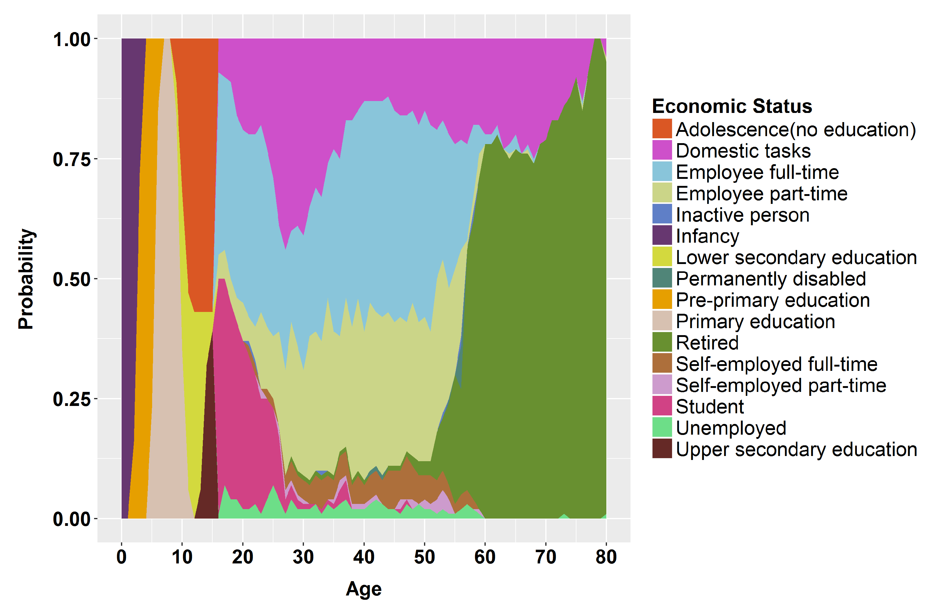
Figure 1 shows the life course trajectory of a German, female, retired, aged 80 in 2010 as an example. The model predicts the probability of the economic status for each year of an individual‘s lifespan. The results of exposure modelling for each past year was linked with this model to assess the lifelong exposure. More detailed information for the life course trajectory model can be found in the ad hoc HEALS deliverable [52].
2.4. Validation with Measurement Data
A wide range of input data for the parameters of the mass-balance model has been reported by different studies. Hence, it is necessary to carry out a thorough data collection and validate the modelling results with the monitoring data. The authors selected the data from project EXPOLIS to validate the modelling results for indoor concentration at home. EXPOLIS was a multi-centre study in Europe which monitored the concentration of PM2.5 and NO2 home indoor and outdoor in Athens, Basel, Grenoble, Helsinki, Milan and Prague [53]. The measured outdoor concentrations from EXPOLIS, as well as the time-activity patterns from MTUS and other model parameters, were applied to the mass-balance model to simulate the indoor pollutant concentrations. The output of model simulation, which is available as probability density function, is compared with the corresponding indoor measured value. If the simulated values show a low agreement with the measurement data, a new round of data collection is carried out to adjust the input data for model parameters until a high match can be reached.
3. Results
3.1. Annual Average Exposure
3.1.1. PM2.5
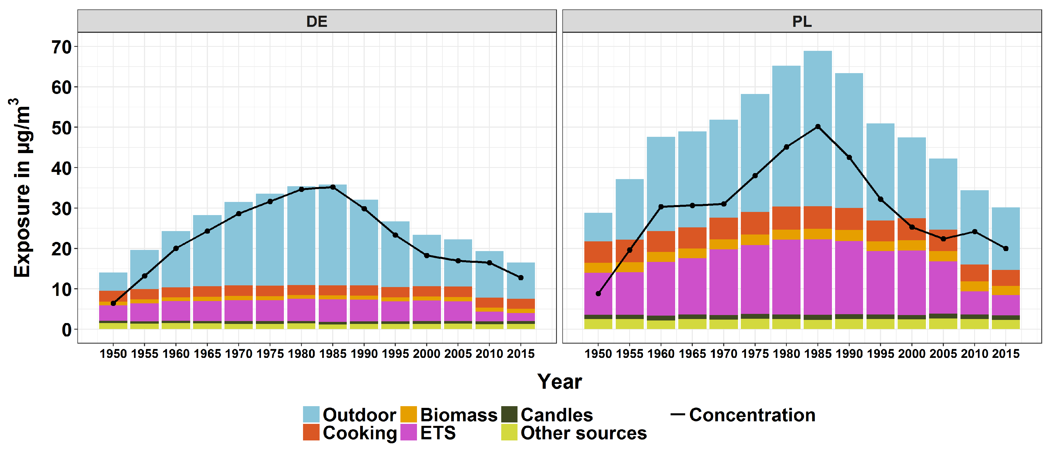
As a starting point, the authors simulated the annual exposure to both pollutants since the 1950s. Figure 2 shows the population-weighted arithmetic mean of the PM2.5 exposure in Germany and Poland stratified by source, including infiltration from outdoors, cooking, wood burning, smoking, candle/incense burning and other sources. The black line in the figure represents the population-weighted average PM2.5 ambient concentrations in the two countries.
It can be seen from the plot that for both countries, the trend of the total exposure matches well with the temporal course of the ambient concentration. For the two countries, the exposure, as well as the background concentration kept increasing from 1950 to a peak in 1985 and fell down notably until 2015. This decrease was mainly originated from the implementation of a series of emission reduction measures for PM2.5 and its precursors in Europe (e.g., the Air Quality Directives and EURO Standards for Vehicles) [54].
Moreover, a sharp decrease of exposure stemming from ETS in 2010 for both countries can be observed. The reason behind is the measures that were taken in European countries for tobacco control, including the smoking bans in public places and at workplaces [55]. However, the ETS was still responsible for 17% and 12% of the average exposure in 2015 in Poland and Germany respectively. This value even amounted 36% and 27% in 1950 when the contribution made by outdoor air was relatively small.
Despite the similarities stated above, an apparent gap of the exposure level between the two countries can be observed. Generally, the exposure in Poland is almost twice that of Germany. First of all, the background concentration in Poland was obviously higher than that in Germany, especially between the 1980s and the 1990s. The extremely high PM2.5 ambient concentration in Poland was mainly resulted from its overwhelming reliance on lignite and hard coal in the energy section compared other countries [56]. Since Poland became a member state of the European Union in 2004, this issue has been highly addressed and the government has endeavoured to comply with EU directives [57]. The effectiveness of the measures taken (e.g., renewal of the outdated power plants and construction of new power plants mainly using gas or other renewable energy) can be reflected by the drop of the outdoor PM2.5 concentrations since the 2010s.
Moreover, the exposure due to indoor sources in Poland was higher than that of Germany for all the time periods. The main reason behind is the smaller dwelling size in Poland. According to the EU-SILC data, the average dwelling size in Germany was 104 m2, while this value for Poland was only 85 m2. Although the smaller dwelling size is irrelevant to exposure stemming from outdoor concentration, it slows down the dilution of concentration generated from indoor sources. Last but not least, the longer cooking time and higher prevalence of indoor smoking also led to the higher exposure in Poland.
At the European level, the temporal course of PM2.5 exposure has the similar trend as these two countries. The average exposure in 1950 was at 19.0 (95% CI: 3.3–55.7) µg/m3 and raised to a peak at 37.2 (95% CI: 9.2–113.8) µg/m3 in 1980. Afterward the total exposure kept dropping to 2015 at 20.1 (95% CI: 5.8–51.2) µg/m3. Basically the outdoor air was the greatest contributor to the overall exposure, especially for the peak year with 55%. Except for the outdoor air, indoor smoking and cooking were the most important sources.
3.1.2. NO2
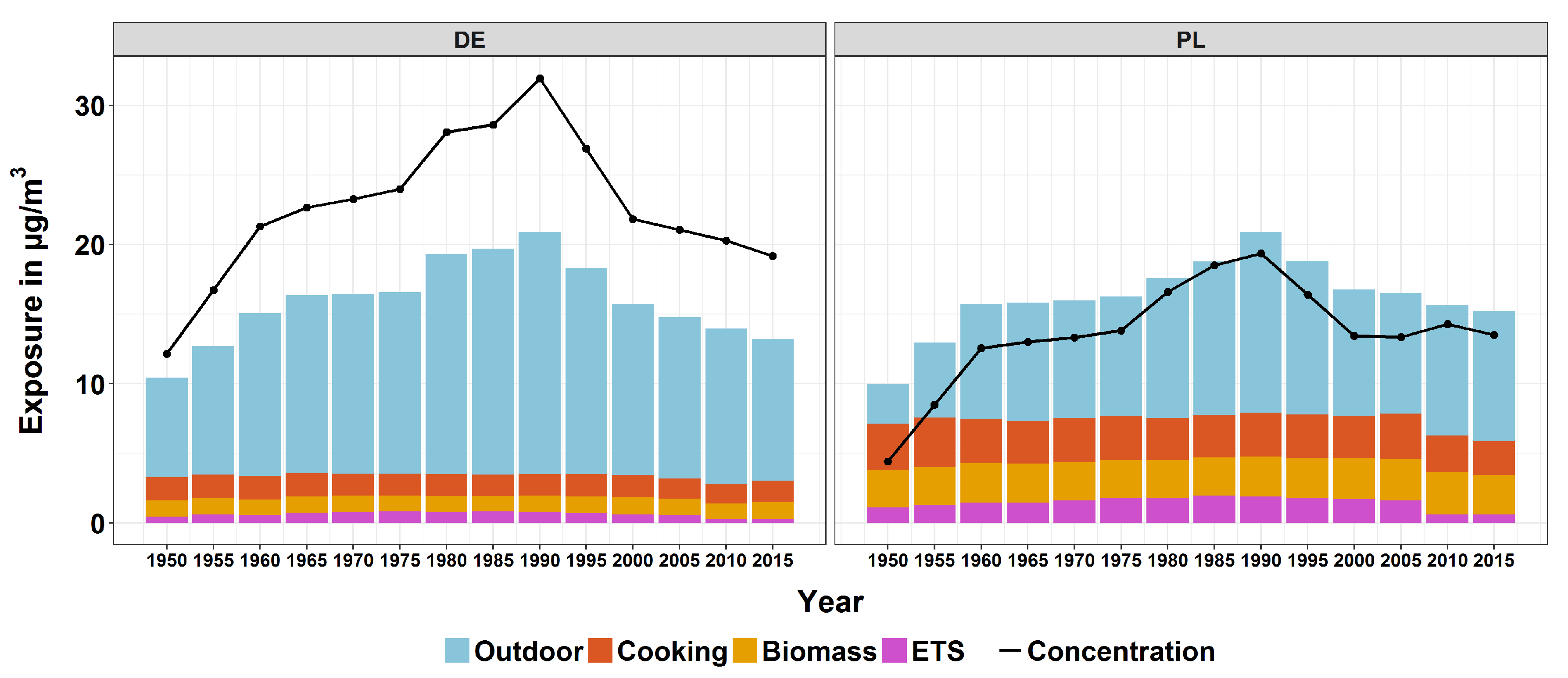
The authors also simulated the temporal course of exposure to NO2 for the EU27+2 countries. Figure 3 displays the population-weighted annual average for Germany and Poland between 1950 to 2015. For both countries, the background concentration and the total exposure kept increasing from 1950 to the highest point in 1990 and then began to decline steadily until 2015. Compared to PM2.5, one obvious difference can be observed is the contribution made by the indoor smoking. Even for Poland with very high prevalence of indoor smoking, the contribution made by ETS was still less than 10% in 1990. The less important role played by ETS for NO2 exposure has also been observed by Koo et al. (1990) [58] and Adgate et al. (1992) [59].
Even though the total exposure levels to NO2 for both countries were similar, their source distribution made a huge difference. The average background concentration in Germany was on average twice that of Poland. As a result, the dominant contribution was made by the outdoor air, especially for the peak year of 1990 (83%). In contrast, the portion occupied by the indoor sources in Poland was relatively high (40% in 1990). Cooking and wood stove became the two main contributors for the indoor generated NO2 concentration.
At European level, the temporal trend was similar to that of Germany and Poland. The lowest level was found in 1950 with 10.4 (95% CI: 0.9–36.8) µg/m3. In 1990 the total exposure reached a peak at 21.4 (95% CI: 6.3–51.8) µg/m3 with 78% contributed by the outdoor air. The overall exposure dropped to 15.5 (95% CI: 4.8–36.8) µg/m3 in 2015 mainly as a result of the decrease of outdoor concentration.
3.2. Exposure by Socio-Demographic Status
As stated previously, the exposure is differentiated between population subgroups that are characterised by socio-demographic features. In this paper, the influence of gender, income level and degree of urbanisation on exposure to both pollutants at European level is discussed.
3.2.1. By Gender
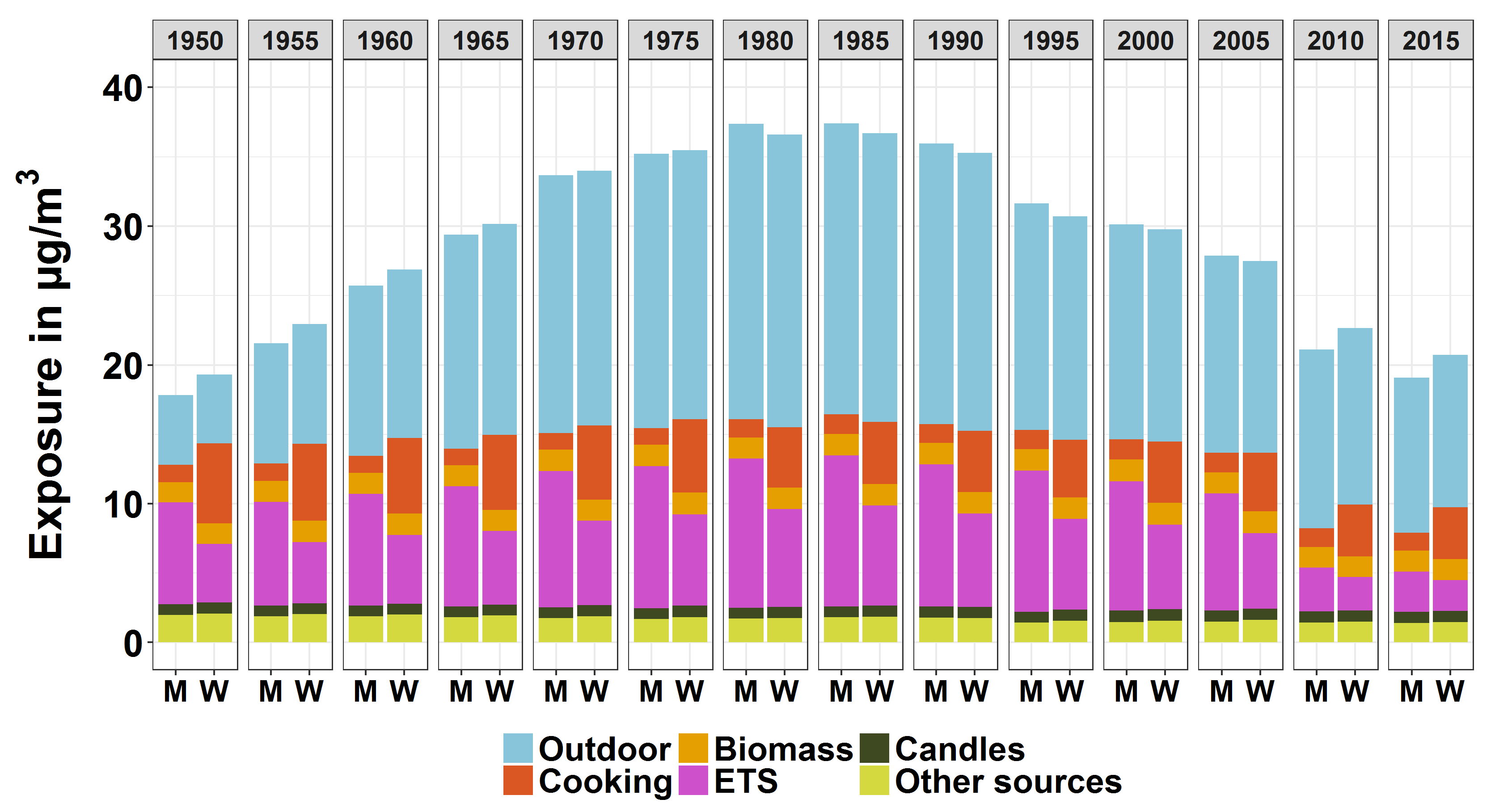
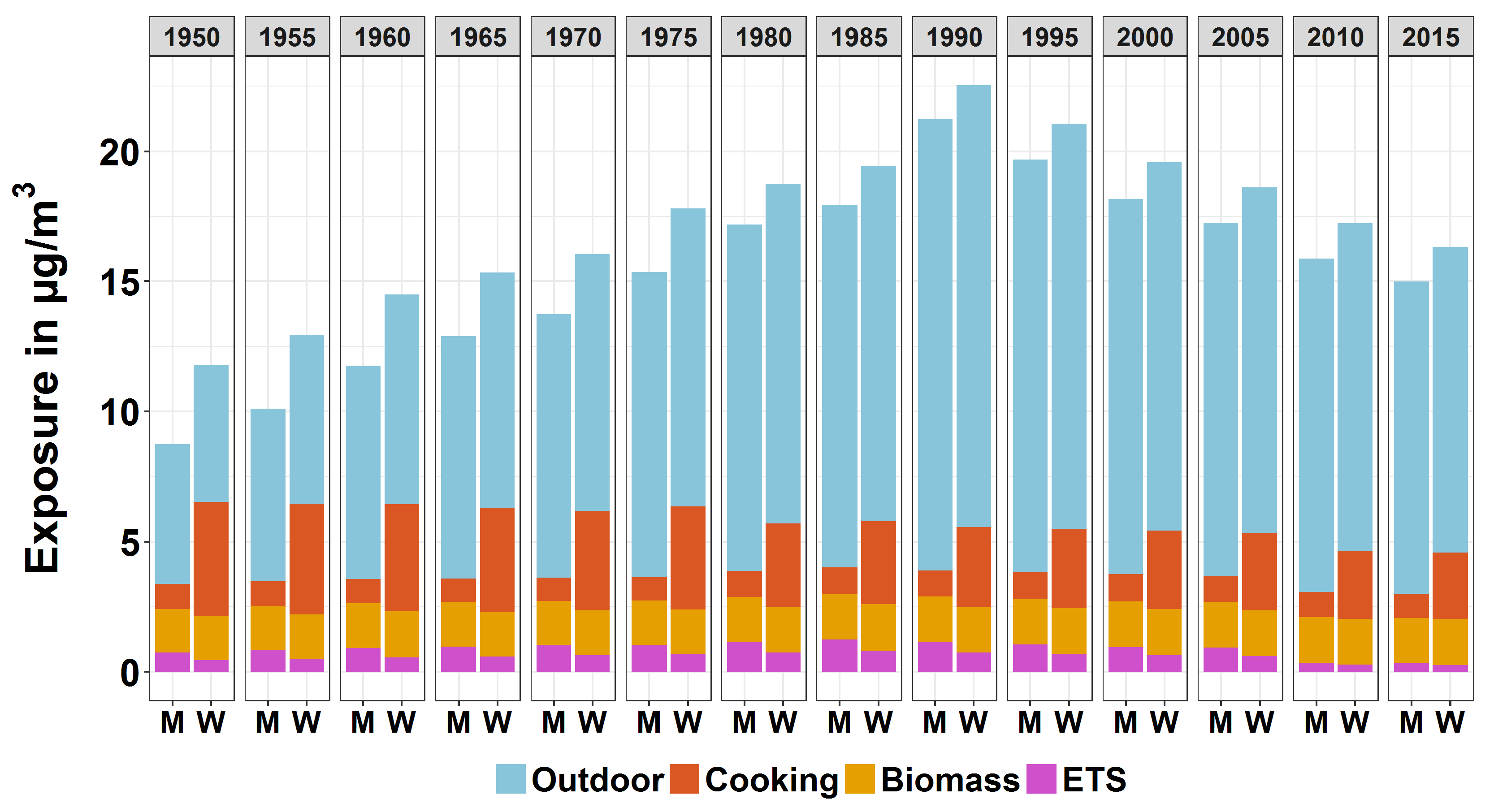
Figure 4 displays the population-weighted arithmetic mean PM2.5 exposure by source and gender for European countries from 1950 to 2015. It can be observed that before 1980 the total exposure burdened by women was higher than that by men. However, the opposite situation took place from the 1980s and lasted until 2010, when females again experienced higher overall exposure to PM2.5.
Very large gaps of exposure owing to ETS and cooking can be seen between women and men. Basically males experienced a higher level of exposure due to ETS as a result of the higher prevalence of smokers and average cigarette consumption [60]. In contrast, the exposure stemming from cooking of women was apparently higher than that of men, especially for the earlier time periods. The MTUS data shows that in 1960 women spent on average 116 min on cooking per day, which was almost 10 times that of men (12 min).
Before 1980, the higher exposure originated from cooking played more important role and as a result women were burdened with heavier exposure to PM2.5, even though they were less affected by indoor smoking. In the following years, however, the gap of exposure from cooking between the two groups decreased and the influence of ETS became more crucial. After 2005, the exposure experienced by women overtook again as a result of the sharp decrease of exposure from smoking due to the implementation of smoking bans in European countries.
Figure 5 shows the population-weighted arithmetic mean NO2 exposure by source and gender for European countries from 1950 to 2015. For NO2, the development of temporal trend is less complicated than for PM2.5—women experienced higher exposure than men for all the time periods. The main reason behind is that the women were exposed to higher level of exposure from cooking. Even though the gaps of exposure stemming from indoor smoking can still be observed, the contribution of smoking to the overall exposure was almost ignorable.
3.2.2. By Income Level
Figure 6 and Figure 7 show the population-weighted arithmetic mean exposure by source and income level for European countries from 1950 to 2015 for PM2.5 and NO2 respectively. The income level was classified into three categories as the “Low” (lowest 25%), “Median” (middle 50%) and “High” (highest 25%).
For both pollutants, the exposures were negatively correlated with the income level. What can be apparently observed by both plots are the differences of exposure from cooking among three subgroups. People with the lowest household income were burdened with the highest exposure due to cooking. On the one hand, the income level was positively related to the residential size. For example, the average dwelling size for Germans with the highest income level was 136 m2, whereas the value for people with lowest income was only 80 m2. Thus, the population with low income were exposed to a higher level of exposure due to indoor sources, including cooking since the smaller room size hindered the dilution of the pollutants.
On the other hand, the people with low income tended to spend more time on cooking. According to the MTUS data, women with high income spent on average 84 min per day on cooking in the 1980s, while the cooking time for women with low income amounted to 109 min. The longer cooking time also increased the exposure from cooking to both pollutants for the low income group.
3.2.3. By Degree of Urbanisation
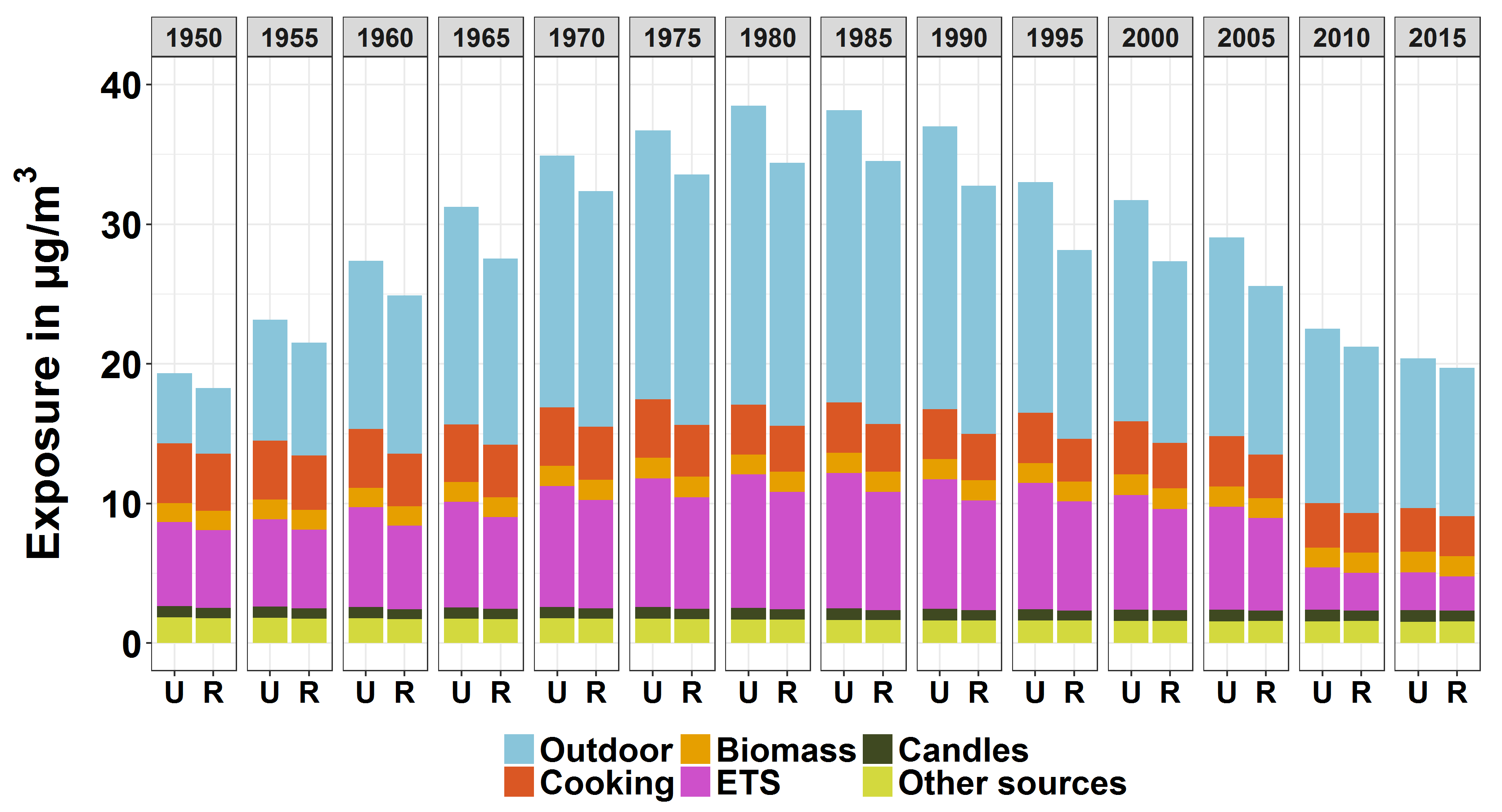
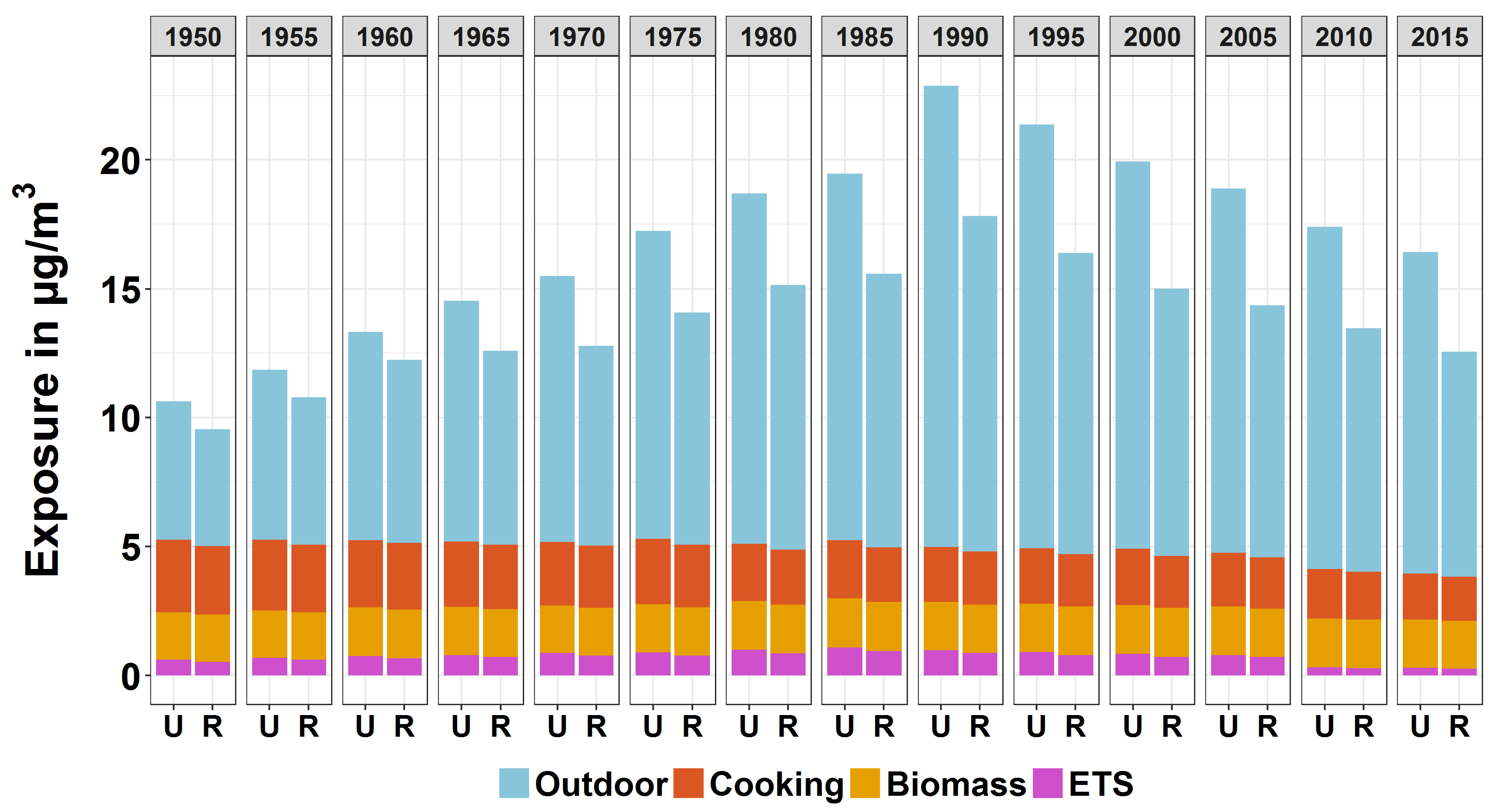
Figure 8 and Figure 9 show the population-weighted arithmetic mean exposure by source and degree of urbanisation for European countries from 1950 to 2015 for PM2.5 and NO2 respectively. The total exposures to both pollutants in urban or suburban areas were higher than that in rural areas, especially for NO2.
What can be seen in both figures is the apparent heavier exposure due to the outdoor air in the cities as a result of the urban increment. Urban increment is the remarkably higher concentration of pollutant in urban areas. This is particularly an issue for NO2 since motor vehicles are important sources for NO2 emission in urban areas. Meanwhile, it is not surprising that people in urban areas tended to reside in smaller dwellings. According to the EU-SILC data, the average residence size of the Germans in urban areas was 103 m2, while for people in rural areas this value reached 123 m2. The smaller room size in urban and suburban areas led to a higher exposure originated from indoor sources.
3.2.4. Lifelong Exposure
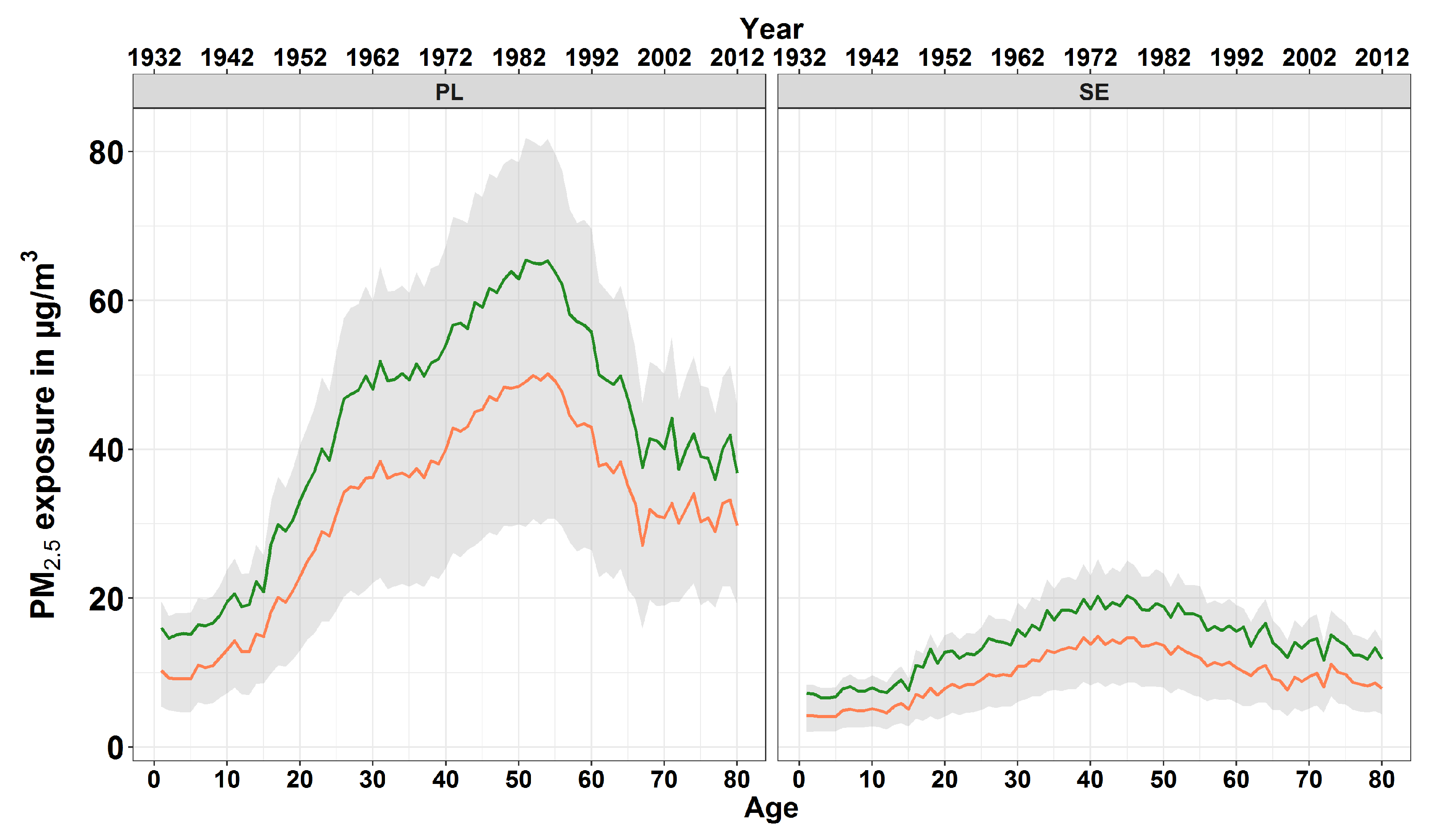
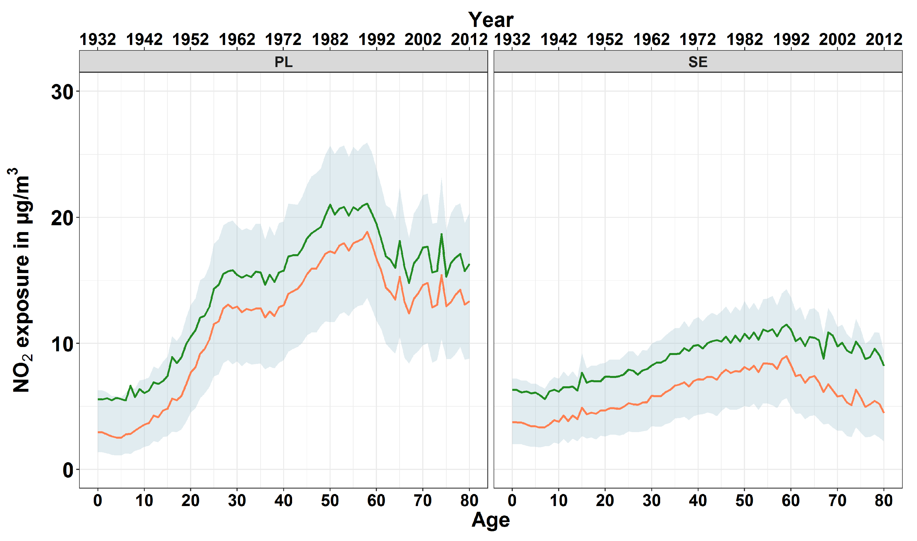
With the support of the life course trajectory model, the lifelong exposures to both pollutants for the eldest cohorts of the population data, that is, 80 years of age were simulated. Large variances of exposure level were observed among different countries. Figure 10 shows the comparison of the temporal course of the lifelong exposure to PM2.5 for the 80-year-old male from Poland and Sweden. The exposure to PM2.5 of the Polish male was apparently higher than that of the Swedish male for each year of lifetime. The average exposure over lifetime for a Polish man was 42.22 (95% CI: 3.38–153.58) µg/m3, whereas for a Swedish man the value was only 14.03 (95% CI: 1.33–54.14) µg/m3. Even though the difference between the two countries was less obvious, the average exposure to NO2 for the Polish man (12.55, 95% CI: 0.75–39.06 µg/m3) was still over 50% higher than that of the Swedish man (8.10, 95% CI: 0.62–33.79 µg/m3) (see Figure 11).
At European level, the average exposure to PM2.5 over lifetime for an 80-year-old reached 23.86 (95% CI: 2.95–81.86) µg/m3, within which 53% was originated from the indoor sources. The average exposure to NO2 amounted to 13.49 (95% CI: 1.36–43.84) µg/m3 with more crucial role played by the infiltration from outdoors (67%).
3.2.5. Validation
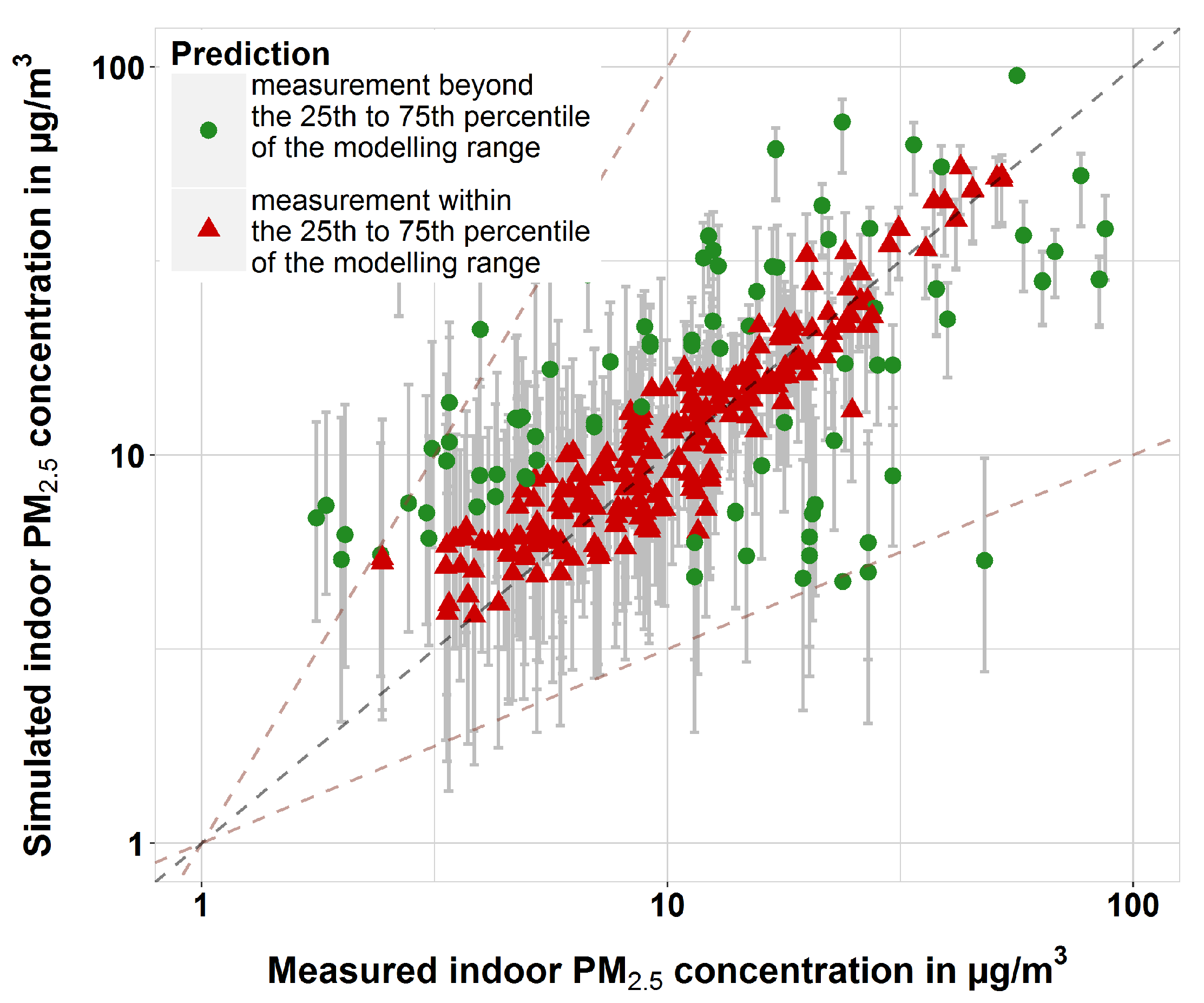
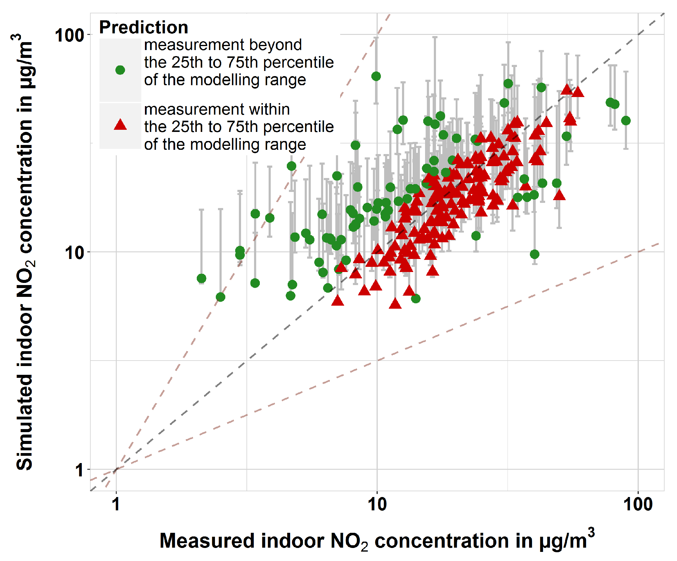
As stated previously, the measurement data from EXPOLIS were employed to validate the parameters of mass-balance model for dwellings. The estimation is considered “good performance” if the monitoring indoor concentration is within the range of 25th to 75th percentile of the predicting result. Multiple rounds of data collection and adjustment have been conducted and the results of validation are presented in Figure 12 and Figure 13. 70% (258 out of 370) and 65% (172 out of 265) of the dots for PM2.5 and NO2 are within the acceptable range.
4. Discussion
Despite the large efforts that have been made within the last few decades, Europe is still facing the challenges of severe health impacts brought about by PM2.5 and NO2. However, the existing epidemiological studies only related the health outcomes to outdoor air concentration, which ignored the impacts of personal activity pattern, building characteristics and indoor pollutant sources. Also, the health status of a person is determined by the lifelong exposure rather than the exposure within a short time period. Thus, to estimate the health impacts, the long-term exposure to pollutants has to be known, which means a model to simulate the long-term exposure is necessary.
To achieve this goal, the authors developed a methodological framework to quantify the annual exposures to PM2.5 and NO2 of the whole lifetime for individuals and population subgroups with certain characteristics. The subgroups were characterised by a number of indicators such as age, gender, socio-economic status, location of workplace and home and behavioural patterns. To estimate the exposure for each year, the authors developed a probabilistic model to simulate the concentration of pollutants in different micro-environments, including outdoors, indoors and in transportation. The contribution of indoor sources, including cooking, smoking, wood burning, candle/incense and other sources was evaluated.
Large variances have been observed by the exposure to PM2.5 and NO2 among different countries. Generally, the exposure in Eastern European countries (e.g., Poland) ranked in the top of all the simulated countries. First of all, these countries suffered very high background concentration. For Poland, this was partly originated from the dependence on lignite and hard coal in the energy industry—over 1/3 of the domestic electricity has been generated by the lignite-fired power plants [61]. The combustion of lignite and hard coal by the professional power industry results in a large amount of emission of PM2.5 and its precursors (e.g., NOx and SO2) [62]. Besides, the Eastern European countries reported comparably higher prevalence of indoor smoking and longer time spent on cooking, which resulted in higher exposure from indoor smoking and cooking. For example, 24% of the people in Poland were exposed to indoor smoking, while only 2% of the people in Finland were affected. With respect to cooking time, it is found that the women in Eastern Europe spent on average 68% more time on cooking than women in Northern Europe in 2000 (105 min for Eastern Europe and 63 min for Northern Europe). Last but not least, the smaller dwelling size compared to the countries was also an important reason. Even though the smaller room size is irrelevant to the exposure from infiltration, it hinders the dilution of the indoor sources.
At European level, the annual average exposure to PM2.5 showed a steady trend of increase since the 1950s from 19.0 (95% CI: 3.3–55.7) µg/m3 to a maximum of 37.2 (95% CI: 9.2–113.8) µg/m3 in the 1980s. The exposure turned to decline gradually afterwards until 2015 to 20.1 (95% CI: 5.8–51.2) µg/m3. The exposure to NO2 followed the similar trend with a peak value in the 1990s at 21.4 (95% CI: 6.3–51.8) µg/m3. In contrast, the average exposures in 1950 and 2015 were only 10.4 (95% CI: 0.9–36.8) and 15.5 (95% CI: 4.8–36.8) µg/m3. One main reason for the drop of exposure after the peak years was the implementation of a series of emission reduction policies for PM2.5 and its precursors (NOx, NH3 and SO2) since the 1970s (e.g., the Air Quality Directives and the EURO Standards for Vehicles), which introduced the continuous decrease of ambient pollutant concentration.
Basically, the outdoor air was an important contributor to the overall exposure, especially for the peak years (55% for PM2.5 and 78% for NO2). However, the influence of indoor sources should not be ignored. For PM2.5, the most important indoor source was the ETS, which was responsible for 23% of the total exposure in 1980. However, the role played by ETS dropped sharply to only 12% after 2010 due to the introduction of indoor smoking bans. For NO2 exposure the role played by ETS was very limited, while cooking and wood burning turned out to be the crucial sources.
The influence of the socio-demographic factors, including gender, income level, together with degree of urbanisation on exposure to both pollutants were addressed. Regarding gender, the exposure due to ETS and cooking showed apparent differences. With respect to cooking, it is not surprising that women were more influenced especially in the earlier time periods. While for smoking, men suffered heavier exposure as a result of higher prevalence of smokers and daily cigarette consumption.
For both pollutants, the highest exposures were experienced by the population with the lowest income level. This finding was mainly resulted from the smaller dwelling size of the low-income group. As discussed previously, the tiny room slows down the dilution of pollution generated from indoor sources. Also the longer cooking time of the people with low income increased the overall exposure to both pollutants.
People living in urban areas experienced higher level of exposure, especially to NO2, than people in rural areas. The background concentration in cities was greatly elevated due to the heavy traffic. Moreover, the smaller average dwelling size of the urban citizens is another important reason for the advancement of the exposure due to indoor sources.
The authors also conducted the simulation to assess the lifelong exposure to both pollutants for the people that are 80 years old in Europe. Again very large differences have been observed among different countries. The comparison shows that the average PM2.5 exposure of lifetime for a Polish man was over 3 times that of a Swedish man. Even though the gap was less obvious, the average NO2 exposure of the Polish man was still 50% higher than that of the Swedish man. Generally, the average exposure over lifetime to PM2.5 and NO2 was 23.86 (95% CI: 2.95–81.86) and 13.49 (95% CI: 1.36–43.84) µg/m3 respectively.
Last but not least, the authors validated the mass-balance model for simulating the concentration indoors at home with the measurement data from the project EXPOLIS. The adjusted model results reached very high agreement with the monitoring data. For PM2.5 and NO2, 70% and 65% of the measurement samples were falling within the range of the 25th to 75th percentile of the simulated outcome.
5. Conclusions
The methodology framework developed in this publication is applicable to European countries to simulate the lifelong exposure to PM2.5 and NO2 for different socio-demographic subgroups. The method integrated the indoor sources, including cooing, smoking, wood burning, candles/incense and other sources to the traditional exposure models. Meanwhile, it considered the influence of the reduction measures (e.g., smoking bans and cooking hoods) on the exposure levels. The model was validated with the measurement data and reached high agreement with the monitoring values. Last but not least, the incorporation of the life course trajectory model for assessing the lifelong exposure brought new ideas to the assessment of health impacts and environmental policies.
Still there is great potential for future improvement. Many studies have revealed high pollutant concentration in restaurants and bars. It is worthwhile if these micro-environments could be additionally addressed. Moreover, many studies have pointed out the large variance of pollutant concentration among different modes of transportation. Thus to highlight the different modes could be advantageous. Besides, to increase the temporal resolution of the model input data, for example, the background concentration and the air exchange rate would be helpful. Last but not least, it should be improved in the future that if the life course trajectories for other socio-economic variables, for example, income level, civil status, could be covered.
Author Contributions
Conceptualization, N.L. and R.F.; Data curation, N.L.; Formal analysis, R.F.; Funding acquisition, R.F.; Investigation, N.L.; Methodology, N.L.; Project administration, R.F.; Software, N.L.; Supervision, R.F.; Validation, N.L.; Visualization, N.L.; Writing—original draft, N.L.; Writing—review & editing, R.F.
Funding
This research was funded by Seventh Framework Programme project HEALS (grant number FP7-ENV-603946) and Horizon 2020 project ICARUS (grant agreement number 690105).
Acknowledgments
The authors want to express our special thanks to Christian Schieberle for his contribution of the life course trajectory model. Additionally, the authors want to express their gratitude to EUROSTAT for providing the EU-SILC microdata, which was utilised as the input data for life course trajectory model.
Conflicts of Interest
The authors declare no conflict of interest.
References
- WHO. Health Risks of Air Pollution in Europe—HRAPIE Project: Recommendations for Concentration-Response Functions for Cost-Benefit Analysis of Particulate Matter, Ozone and Nitrogen Dioxide; Technical Report; WHO Regional Office for Europe: Copenhagen, Denmark, 2013.
- Polichetti, G.; Cocco, S.; Spinali, A.; Trimarco, V.; Nunziata, A. Effects of particulate matter (PM10, PM2.5 and PM1) on the cardiovascular system. Toxicology 2009, 261, 1–8. [Google Scholar] [CrossRef] [PubMed]
- Wang, C.; Tu, Y.; Yu, Z.; Lu, R. PM2.5 and cardiovascular diseases in the elderly: An overview. Int. J. Environ. Res. Public Health 2015, 12, 8187–8197. [Google Scholar] [CrossRef] [PubMed]
- Ha, E.H.; Hong, Y.C.; Lee, B.E.; Woo, B.H.; Schwartz, J.; Christiani, D.C. Is air pollution a risk factor for low birth weight in Seoul? Epidemiology 2001, 12, 643–648. [Google Scholar] [CrossRef] [PubMed]
- Cibella, F.; Cuttitta, G.; Della Maggiore, R.; Ruggieri, S.; Panunzi, S.; de Gaetano, A.; Bucchieri, S.; Drago, G.; Melis, M.R.; la Grutta, S.; et al. Effect of indoor nitrogen dioxide on lung function in urban environment. Environ. Res. 2015, 138, 8–16. [Google Scholar] [CrossRef] [PubMed] [Green Version]
- Kruize, H.; Hänninen, O.; Breugelmans, O.; Lebret, E.; Jantunen, M. Description and demonstration of the EXPOLIS simulation model: Two examples of modeling population exposure to particulate matter. J. Expo. Sci. Environ. Epidemiol. 2003, 13, 87–99. [Google Scholar] [CrossRef] [PubMed]
- Brunekreef, B.; Janssen, N.A.; de Hartog, J.J.; Oldenwening, M.; Meliefste, K.; Hoek, G.; Lanki, T.; Timonen, K.L.; Vallius, M.; Pekkanen, J.; et al. Personal, indoor, and outdoor exposures to PM2.5 And its components for groups of cardiovascular patients in Amsterdam And Helsinki. Res. Rep. Health Eff. Inst. 2005, 127, 1–70. [Google Scholar]
- Hänninen, O.; Hoek, G.; Mallone, S.; Chellini, E.; Katsouyanni, K.; Gariazzo, C.; Cattani, G.; Marconi, A.; Molnár, P.; Bellander, T.; et al. Seasonal patterns of outdoor PM infiltration into indoor environments: Review and meta-analysis of available studies from different climatological zones in Europe. Air Qual. Atmos. Health 2011, 4, 221–233. [Google Scholar] [CrossRef]
- Burke, J.M. SHEDS-PM Stochastic Human Exposure and Dose Simulation for Particulate Matter, Users Guide EPA SHEDS-PM 2.1; Technical Report EPA/600/R-05/065; U.S. Environmental Protection Agency: Washington, DC, USA, 2005.
- Gens, A. Modelling the Exposure to Fine Particles and Its Impacts on Human Health in Europe. Ph.D. Thesis, University of Stuttgart, Stuttgart, Germany, 2012. [Google Scholar]
- US EPA. Air Pollutants Exposure Model Documentation (APEX, Version 5); Technical Report EPA-452/R-17-001; U.S. Environmental Protection Agency: Washington, DC, USA, 2017.
- Burke, J.M.; Zufall, M.J.; Özkaynak, H. A population exposure model for particulate matter: Case study results for PM2.5 in Philadelphia, PA. J. Expo. Sci. Environ. Epidemiol. 2001, 11, 470–489. [Google Scholar] [CrossRef]
- Branis, M.; Linhartova, M. Association between unemployment, income, education level, population size and air pollution in Czech cities: Evidence for environmental inequality? A pilot national scale analysis. Health Place 2012, 18, 1110–1114. [Google Scholar] [CrossRef]
- Byun, H.; Bae, H.; Kim, D.; Shin, H.; Yoon, C. Effects of socioeconomic factors and human activities on children’s PM10 exposure in inner-city households in Korea. Int. Arch. Occup. Environ. Health 2010, 83, 867–878. [Google Scholar] [CrossRef]
- Georgopoulos, P.; Lioy, P.J. Conceptual and theoretical aspects of human exposure and dose assessment. J. Expo. Anal. Environ. Epidemiol. 1994, 4, 253–285. [Google Scholar]
- Duan, N. Models for human exposure to air pollution. Environ. Int. 1982, 8, 305–309. [Google Scholar] [CrossRef]
- Lioy, P.; Weisel, C. Exposure Science: Basic Principles and Applications; Academic Press: Cambridge, MA, USA, 2014. [Google Scholar]
- Fisher, K.; Gershuny, J. Multinational Time Use Study: User’s Guide and Documentation, version 9; Technical Report; Centre for Time Use Research: Oxford, UK, 2016. [Google Scholar]
- Tainio, M.; Tuomisto, J.T.; Pekkanen, J.; Karvosenoja, N.; Kupiainen, K.; Porvari, P.; Sofiev, M.; Karppinen, A.; Kangas, L.; Kukkonen, J. Uncertainty in health risks due to anthropogenic primary fine particulate matter from different source types in Finland. Atmos. Environ. 2010, 44, 2125–2132. [Google Scholar] [CrossRef]
- Arunraj, N.S.; Mandal, S.; Maiti, J. Modeling uncertainty in risk assessment: An integrated approach with fuzzy set theory and Monte Carlo simulation. Accid. Anal. Prev. 2013, 55, 242–255. [Google Scholar] [CrossRef] [PubMed]
- Simpson, D.; Benedictow, A.; Berge, H.; Bergström, R.; Emberson, L.D.; Fagerli, H.; Flechard, C.R.; Hayman, G.D.; Gauss, M.; Jonson, J.E.; et al. The EMEP MSC-W chemical transport model-technical description. Atmos. Chem. Phys. 2012, 12, 7825–7865. [Google Scholar] [CrossRef]
- Horálek, J.; Denby, B.; de Smet, P.; de Leeuw, F.; Kurfürst, P.; Swart, R.; van Noije, T. Spatial Mapping of Air Quality for European Scale Assessment; Technical Report ETC/ACC Technical Paper 2006/6; European Topic Centre on Air and Climate Change: Bilthoven, The Netherlands, 2007. [Google Scholar]
- Horálek, J.; de Smet, P.; de Leeuw, F.; Kurfürst, P. European NO2 Air Quality Map for 2014; Technical Report ETC/ACM Technical Paper 2017/6; European Topic Centre on Air and Climate Change: Bilthoven, The Netherlands, 2017. [Google Scholar]
- McKeen, S.; Wilczak, J.; Grell, G.; Djalalova, I.; Peckham, S.; Hsie, E.Y.; Gong, W.; Bouchet, V.; Menard, S.; Moffet, R.; et al. Assessment of an ensemble of seven real-time ozone forecasts over eastern North America during the summer of 2004. J. Geophys. Res. Atmos. 2005, 110, D21. [Google Scholar] [CrossRef]
- Van Aardenne, J.A.; Dentener, F.J.; Olivier, J.G.J.; Klein Goldewijk, C.G.M.; Lelieveld, J. A 1°×1° resolution data set of historical anthropogenic trace gas emissions for the period 1890–1990. Glob. Biogeochem. Cycles 2001, 15, 909–928. [Google Scholar] [CrossRef]
- University of Stuttgart. EcoSense Web2. 2018. Available online: http://ecosenseweb.ier.uni-stuttgart.de (accessed on 1 September 2018).
- Schieberle, C.; Li, N.; Friedrich, R. Report on the Development of a Probabilistic Exposure Modelling Framework to Assess External Exposure to Chemicals for Selected Population Groups; Technical Report; HEALS Consortium: Paris, France, 2016. [Google Scholar]
- Thornburg, J.; Ensor, D.S.; Rodes, C.E.; Lawless, P.A.; Sparks, L.E.; Mosley, R.B. Penetration of particles into buildings and associated physical factors. Part I: Model development and computer simulations. Aerosol Sci. Technol. 2001, 34, 284–296. [Google Scholar] [CrossRef]
- Földváry, V.; Bekö, G.; Langer, S.; Arrhenius, K.; Petráš, D. Effect of energy renovation on indoor air quality in multifamily residential buildings in Slovakia. Build. Environ. 2017, 122, 363–372. [Google Scholar] [CrossRef] [Green Version]
- Hänninen, O.O.; Lebret, E.; Ilacqua, V.; Katsouyanni, K.; Künzli, N.; Srám, R.J.; Jantunen, M. Infiltration of ambient PM2.5 and levels of indoor generated non-ETS PM2.5 in residences of four European cities. Atmos. Environ. 2004, 38, 6411–6423. [Google Scholar] [CrossRef]
- University of Western Macedonia. OFFICAIR Modelling System. 2013. Available online: http://www.officair-project.eu (accessed on 1 May 2012).
- Oezkaynak, H.; Xue, J.; Weker, R.; Butler, D.; Koutrakis, P. Particle Team (PTEAM) Study: Analysis of the Data—Final Report, Volume 3; Technical Report EPA/600/R-95/098; U.S. Environmental Protection Agency: Washington, DC, USA, 1996.
- Fabian, P.; Adamkiewicz, G.; Levy, J.I. Simulating indoor concentrations of NO2 and PM2.5 in multifamily housing for use in health-based intervention modeling. Indoor Air 2012, 22, 12–23. [Google Scholar] [CrossRef] [PubMed]
- Yang, W.; Lee, K.; Chung, M. Characterization of indoor air quality using multiple measurements of nitrogen dioxide. Indoor Air 2004, 14, 105–111. [Google Scholar] [CrossRef] [PubMed]
- Thornburg, J.W.; Rodes, C.E.; Lawless, P.A.; Stevens, C.D.; Williams, R.W. A pilot study of the influence of residential HAC duty cycle on indoor air quality. Atmos. Environ. 2004, 38, 1567–1577. [Google Scholar] [CrossRef]
- Zhao, P.; Siegel, J.A.; Corsi, R.L. Ozone removal by HVAC filters. Atmos. Environ. 2007, 41, 3151–3160. [Google Scholar] [CrossRef]
- MacIntosh, D.L.; Minegishi, T.; Kaufman, M.; Baker, B.J.; Allen, J.G.; Levy, J.I.; Myatt, T.A. The benefits of whole-house in-duct air cleaning in reducing exposures to fine particulate matter of outdoor origin: A modeling analysis. J. Expo. Sci. Environ. Epidemiol. 2010, 20, 213–224. [Google Scholar] [CrossRef] [PubMed]
- Fortmann, R.; Kariher, P.; Clayton, R. Indoor Air Quality: Residential Cooking Exposures—Final Report; Technical Report 97-300; California Air Resources Board: Sacramento, CA, USA, 2001.
- Struschka, M.; Kilgus, D.; Springmann, M.; Baumbach, G. Effiziente Bereitstellung aktueller Emissionsdaten für die Luftreinhaltung. Texte 2008, 205, 322. [Google Scholar]
- Daisey, J.M.; Mahanama, K.R.R.; Hodgson, A.T. Toxic Volatile Organic Compounds in Environmental Tobacco Smoke: Emission Factors for Modeling Exposures of California Populations; Technical Report LBL-36379; California Air Resources Board: Sacramento, CA, USA, 1994.
- Rickert, W.S.; Robinson, J.C.; Collishaw, N.E. A study of the growth and decay of cigarette smoke NOx in ambient air under controlled conditions. Environ. Int. 1987, 13, 399–408. [Google Scholar] [CrossRef]
- Searl, A. A Review of the Acute and Long Term Impacts of Exposure to Nitrogen Dioxide in the United Kingdom; Technical Report TM/04/03; Institute of Occupational Medicine: Edinburgh, UK, 2004. [Google Scholar]
- He, C.; Morawska, L.; Hitchins, J.; Gilbert, D. Contribution from indoor sources to particle number and mass concentrations in residential houses. Atmos. Environ. 2004, 38, 3405–3415. [Google Scholar] [CrossRef]
- Hu, T.; Singer, B.C.; Logue, J.M. Compilation of Published PM2.5 Emission Rates For Cooking, Candles and Incense for Use in Modeling of Exposures in Residences; Technical Report LBNL-5890E; Lawrence Berkeley National Laboratory: Alameda, CA, USA, 2012. [Google Scholar]
- Ferro, A.R.; Kopperud, R.J.; Hildemann, L.M. Source strengths for indoor human activities that resuspend particulate matter. Environ. Sci. Technol. 2004, 38, 1759–1764. [Google Scholar] [CrossRef]
- Adams, H.S.; Nieuwenhuijsen, M.J.; Colvile, R.N.; McMullen, M.A.S.; Khandelwal, P. Fine particle (PM2.5) personal exposure levels in transport microenvironments, London, UK. Sci. Total Environ. 2001, 279, 29–44. [Google Scholar] [CrossRef]
- Briggs, D.J.; de Hoogh, K.; Morris, C.; Gulliver, J. Effects of travel mode on exposures to particulate air pollution. Environ. Int. 2008, 34, 12–22. [Google Scholar] [CrossRef] [PubMed]
- Zagury, E.; le Moullec, Y.; Momas, I. Exposure of Paris taxi drivers to automobile air pollutants within their vehicles. Occup. Environ. Med. 2000, 57, 406–410. [Google Scholar] [CrossRef] [PubMed] [Green Version]
- Riediker, M.; Williams, R.; Devlin, R.; Griggs, T.; Bromberg, P. Exposure to particulate matter, volatile organic compounds, and other air pollutants inside patrol cars. Environ. Sci. Technol. 2003, 37, 2084–2093. [Google Scholar] [CrossRef] [PubMed]
- Van Roosbroeck, S.; Wichmann, J.; Janssen, N.A.H.; Hoek, G.; van Wijnen, J.H.; Lebret, E.; Brunekreef, B. Long-term personal exposure to traffic-related air pollution among school children, a validation study. Sci. Total Environ. 2006, 368, 565–573. [Google Scholar] [CrossRef] [PubMed] [Green Version]
- Zuurbier, M.; Hoek, G.; Oldenwening, M.; Lenters, V.; Meliefste, K.; van den Hazel, P.; Brunekreef, B. Commuters’ exposure to particulate matter air pollution is affected by mode of transport, fuel type, and route. Environ. Health Perspect. 2010, 118, 783–789. [Google Scholar] [CrossRef] [PubMed]
- Schieberle, C.; Li, N.; Friedrich, R. Report on the Application of the Exposure Modeling Framework To Population Studies Covered in Stream 5; Technical Report; HEALS Consortium: Paris, France, 2017. [Google Scholar]
- Jantunen, M.J.; Hänninen, O.; Katsouyanni, K.; Knöppel, H.; Kuenzli, N.; Lebret, E.; Maroni, M.; Saarela, K.; Sram, R.; Zmirou, D. Air pollution exposure in European cities: The ‘EXPOLIS’ study. J. Expo. Anal. Environ. Epidemiol. 1998, 8, 495–518. [Google Scholar]
- Granier, C.; Bessagnet, B.; Bond, T.; d’Angiola, A.; van der Gon, H.D.; Frost, G.J.; Heil, A.; Kaiser, J.W.; Kinne, S.; Klimont, Z.; et al. Evolution of anthropogenic and biomass burning emissions of air pollutants at global and regional scales during the 1980–2010 period. Clim. Chang. 2011, 109, 163–190. [Google Scholar] [CrossRef]
- Hammond, D. Health warning messages on tobacco products: A review. Tob. Control 2011, 20, 327–337. [Google Scholar] [CrossRef]
- Vasev, N. Governing energy while neglecting health—The case of Poland. Health Policy 2017, 121, 1147–1153. [Google Scholar] [CrossRef]
- Zelljadt, E.; Velten, E.K.; Prahl, A.; Duwe, M.; Poblocka, A. Assessment of Climate Change Policies in the Context of the European Semester, Country Report: Poland; Technical Report Country Reports 2014; Ecologic Institute: Berlin, Germany, 2014. [Google Scholar]
- Koo, L.C.; Ho, J.H.C.; Ho, C.V.; Matsuki, H.; Shimizu, H.; Mori, T.; Tominaga, S. Personal exposure to nitrogen dioxide and its association with respiratory illness in Hong Kong. Am. Rev. Respir. Dis. 1990, 141, 1119–1126. [Google Scholar] [CrossRef]
- Adgate, J.L.; Reid, H.F.; Morris, R.; Helms, R.W.; Berg, R.A.; Hu, P.C.; Cheng, P.W.; Wang, O.L.; Muelenaer, P.A.; Collier, A.M.; et al. Nitrogen dioxide exposure and urinary excretion of hydroxyproline and desmosine. Arch. Environ. Heal. Int. J. 1992, 47, 376–384. [Google Scholar] [CrossRef] [PubMed]
- Eurobarometer. Tobacco; Technical Report Special Eurobarometer 332; European Commission: Brussels, Belgium, 2010.
- Widera, M.; Kasztelewicz, Z.; Ptak, M. Lignite mining and electricity generation in Poland: The current state and future prospects. Energy Policy 2016, 92, 151–157. [Google Scholar] [CrossRef]
- Uliasz-Bochenczyk, A.; Mokrzycki, E. Emissions from the Polish power industry. Energy 2007, 32, 2370–2375. [Google Scholar] [CrossRef]
Figure 1.
Life course trajectory of a German, female, retired, age of 80 in 2010.

Figure 2.
Population-weighted arithmetic mean PM2.5 exposure by source (infiltration from outdoors, cooking, wood burning, smoking, candle/incense burning and other sources) for Germany and Poland from 1950 to 2015. The black line indicates the average background PM2.5 concentrations in the two countries.

Figure 3.
Population-weighted arithmetic mean NO2 exposure by source (infiltration from outdoors, cooking, wood burning, smoking) for Germany and Poland from 1950 to 2015. The black line indicates the average background NO2 concentration in the two countries.
Figure 3.
Population-weighted arithmetic mean NO2 exposure by source (infiltration from outdoors, cooking, wood burning, smoking) for Germany and Poland from 1950 to 2015. The black line indicates the average background NO2 concentration in the two countries.

Figure 4.
Population-weighted arithmetic mean PM2.5 exposure by source and gender for European countries from 1950 to 2015. The “M” stands for “Men” and “W” stands for “Women”.
Figure 4.
Population-weighted arithmetic mean PM2.5 exposure by source and gender for European countries from 1950 to 2015. The “M” stands for “Men” and “W” stands for “Women”.

Figure 5.
Population-weighted arithmetic mean NO2 exposure by source and gender for European countries from 1950 to 2015. The “M” stands for “Men” and “W” stands for “Women”.
Figure 5.
Population-weighted arithmetic mean NO2 exposure by source and gender for European countries from 1950 to 2015. The “M” stands for “Men” and “W” stands for “Women”.

Figure 6.
Population-weighted arithmetic mean PM2.5 exposure by source and income level for European countries from 1950 to 2015. The “L”, “M” and “H” stand for the “Low”, “Median” and “High” level of income.
Figure 6.
Population-weighted arithmetic mean PM2.5 exposure by source and income level for European countries from 1950 to 2015. The “L”, “M” and “H” stand for the “Low”, “Median” and “High” level of income.

Figure 7.
Population-weighted arithmetic mean NO2 exposure by source and income level for European countries from 1950 to 2015. The “L”, “M” and “H” stand for the “Low”, “Median” and “High” level of income.
Figure 7.
Population-weighted arithmetic mean NO2 exposure by source and income level for European countries from 1950 to 2015. The “L”, “M” and “H” stand for the “Low”, “Median” and “High” level of income.

Figure 8.
Population-weighted arithmetic mean PM2.5 exposure by source and degree of urbanisation for European countries from 1950 to 2015. The “U” stands for “Urban or suburban areas” while the “R” stands for “Rural areas”.
Figure 8.
Population-weighted arithmetic mean PM2.5 exposure by source and degree of urbanisation for European countries from 1950 to 2015. The “U” stands for “Urban or suburban areas” while the “R” stands for “Rural areas”.

Figure 9.
Population-weighted arithmetic mean NO2 exposure by source and degree of urbanisation for European countries from 1950 to 2015. The “U” stands for “Urban or suburban areas” while the “R” stands for “Rural areas”.
Figure 9.
Population-weighted arithmetic mean NO2 exposure by source and degree of urbanisation for European countries from 1950 to 2015. The “U” stands for “Urban or suburban areas” while the “R” stands for “Rural areas”.

Figure 10.
Temporal course of the lifelong exposure to PM2.5 for an 80-year-old male from Poland and Sweden. The green line, red line and grey ribbon represent the mean, median and range of 25th to 75th percentile of the exposure level.
Figure 10.
Temporal course of the lifelong exposure to PM2.5 for an 80-year-old male from Poland and Sweden. The green line, red line and grey ribbon represent the mean, median and range of 25th to 75th percentile of the exposure level.

Figure 11.
Temporal course of the lifelong exposure to NO2 for an 80-year-old male from Poland and Sweden. The green line, red line and grey ribbon represent the mean, median and range of 25th to 75th percentile of the exposure level.
Figure 11.
Temporal course of the lifelong exposure to NO2 for an 80-year-old male from Poland and Sweden. The green line, red line and grey ribbon represent the mean, median and range of 25th to 75th percentile of the exposure level.

Figure 12.
Validation for PM2.5. The red dot represents the measurement that is within the corresponding 25th to 75th percentile of the modelling range, while the green dot is beyond that range. For PM2.5 70% of the dots (258 out of 370) are within the range.
Figure 12.
Validation for PM2.5. The red dot represents the measurement that is within the corresponding 25th to 75th percentile of the modelling range, while the green dot is beyond that range. For PM2.5 70% of the dots (258 out of 370) are within the range.

Figure 13.
Validation for NO2. The red dot represents the measurement that is within the corresponding 25th to 75th percentile of the modelling range, while the green dot is beyond that range. For NO2 65% of the dots (172 out of 265) are within the range.
Figure 13.
Validation for NO2. The red dot represents the measurement that is within the corresponding 25th to 75th percentile of the modelling range, while the green dot is beyond that range. For NO2 65% of the dots (172 out of 265) are within the range.


Table 1.
Values of air exchange rate, penetration factor and decay rate.
| Parameter | Micro- Environment | Pollutant | Building Type | ||
|---|---|---|---|---|---|
| Old | Renovated | New | |||
| (h) | home | - | North-western: 0.83 (±0.46), log-normal | 0.5 (±0.1), log-normal [29] | |
| Southern: 1.29 (±1.09), log-normal | |||||
| Eastern 0.75 (±0.43), log-normal | |||||
| Northern 0.81 (±0.85), log-normal [30] | |||||
| work | (0.1, 0.6, 1.8), triangular [31] | ||||
| p | - | PM2.5 | 0.95 (±0.1), log-normal [32] | ||
| NO2 | 1, constant [33] | ||||
| k (h) | - | PM2.5 | 0.39 (±0.1), log-normal [32] | 0.3 (±0.1), log-normal [10] | |
| NO2 | 0.87 (±0.2), log-normal [33] | 0.63 (±0.15), log-normal [34] | |||
Table 2.
Values of air HVAC system related parameters.
| Parameter | Pollutant | Value |
|---|---|---|
| PM2.5 | 0.1–0.6, uniform [35] | |
| NO2 | 0.05–0.8, uniform [36] | |
| N (h) | - | 5 (±2), log-normal, [35] |
| D | - | Residential: 0–1.0, uniform [35] |
| 0.05–0.8, Non-residential: 0.42, constant [37] |
Table 3.
Values of source strength.
| Activity | Pollutant | Value |
|---|---|---|
| Cooking (µg/min) | PM2.5 | 1125 (±280), normal [12,38] |
| NO2 | 270 (±75), normal (Electric stove) [38] | |
| 1800 (±450), normal (Gas stove) [33] | ||
| Wood burning (µg/kJ) | PM2.5 | 13–146, uniform [39] |
| NO2 | 58–185, uniform [39] | |
| Smoking (µg/cigarette) | PM2.5 | 10950 (±2000), normal [32,40] |
| NO2 | 1930 (±644), normal [41,42] | |
| Candles/incense (µg/min) | PM2.5 | 5.5–910, uniform [43,44] |
| Set table, wash/put away dishes (µg/min) | PM2.5 | 20–180, uniform [43,45] |
| Cleaning/other domestic work (µg/min) | PM2.5 | 90–440, uniform [43,45] |
| Laundry, ironing, clothing repair (µg/min) | PM2.5 | 20–180, uniform [43,45] |
| Imputed personal or household care (µg/min) | PM2.5 | 20–80, uniform [43,45] |
| Wash, dress, care for self (µg/min) | PM2.5 | 20–80, uniform [43,45] |
© 2019 by the authors. Licensee MDPI, Basel, Switzerland. This article is an open access article distributed under the terms and conditions of the Creative Commons Attribution (CC BY) license (http://creativecommons.org/licenses/by/4.0/).
Share and Cite
MDPI and ACS Style
Li, N.; Friedrich, R. Methodology for Estimating the Lifelong Exposure to PM2.5 and NO2—The Application to European Population Subgroups. Atmosphere 2019, 10, 507. https://0-doi-org.brum.beds.ac.uk/10.3390/atmos10090507
AMA Style
Li N, Friedrich R. Methodology for Estimating the Lifelong Exposure to PM2.5 and NO2—The Application to European Population Subgroups. Atmosphere. 2019; 10(9):507. https://0-doi-org.brum.beds.ac.uk/10.3390/atmos10090507
Chicago/Turabian StyleLi, Naixin, and Rainer Friedrich. 2019. "Methodology for Estimating the Lifelong Exposure to PM2.5 and NO2—The Application to European Population Subgroups" Atmosphere 10, no. 9: 507. https://0-doi-org.brum.beds.ac.uk/10.3390/atmos10090507
Note that from the first issue of 2016, this journal uses article numbers instead of page numbers. See further details here.