Tsunami-Launched Acoustic Wave in the Layered Atmosphere: Explicit Formulas Including Electron Density Disturbances

Abstract

The problem of the propagation of acoustic wave disturbance initiated by a boundary condition is used to simulate a disturbance of atmospheric gas caused by a rise of water masses. The boundary condition is a function of a dynamic variable that is defined on the border of the problem domain. In this work, it is chosen in such a way that its parameters and form correspond to disturbances in the gas layer produced by a tsunami wave at the air–water interface. The atmosphere is approximately described as a 1D multilayer gas media with an exponential structure of density in each layer. The boundary conditions are set at the interface between water–air and gas layers. These determine the direction of propagation and the ratio of dynamic variables characterizing an acoustic wave. The relationship between such variables (pressure, density, and velocity) is derived by means of projection operators on the subspaces of the z-evolution operator for each layer. The universal formulas for the perturbation of atmospheric variables in an arbitrary layer are obtained in frequency and time domains. As a result, explicit expressions are derived that determine the spectral composition and vertical velocity, by the stationary phase method, of the acoustic disturbance of the atmosphere at an arbitrary height, including the heights of the ionosphere. In return, this can be used to calculate the ionospheric effect. The effect is described by the explicit formula for electron density evolution, which is the solution of the diffusion equation. This forms a quick algorithm for early diagnostics of tsunami waves.

1. Introduction

The detection and prediction of tsunami waves is an urgent task of modern geophysics [1,2]. Among the various approaches to the problem, a set of investigations aimed at studying the ocean–atmosphere–ionosphere connection is being distinguished. Such an approach allows monitoring this formidable phenomenon using satellite communication systems that provide tomographic images of the distribution of the total electron concentration in the region of the dangerous activity of underwater earthquakes and, accordingly, tsunamis [3].

In [4], convincing arguments were presented in favor of the fact that phenomena occurring in the oceans are an important source of waves in the thermosphere. The transmitting link of the disturbance from surface ocean waves is the atmosphere. The tsunami wave disturbs in the atmosphere acoustic and internal gravitational waves [5], the propagation of which at the heights of the thermosphere is accompanied by the transport of plasma along the lines of force. This in turn affects the total electron concentration [6,7,8,9]. Thereby, the solution of the problem of the propagation of the waves initiated by water–air interface boundary conditions proves to be important both in the diagnostics of atmospheric effects and for the detection of tsunami waves at the initial stage [10]. The solution of the problem of propagating such exited acoustic waves is important since observations show that “the first arrival of a transient signal of tsunami-induced waves occurs at a 100-km altitude just 5 min after the tsunami is generated” [11]. In this paper [11], the authors presented two 2D models. The first one is the inelastic fluid model, the analytical-numerical model in which the background state of the atmosphere is modeled as two-layers with the matching conditions at the interface. These conditions lead to the appearance of a reflected wave. The second one is the compressible fluid model for acoustic-gravity waves, which the authors solved numerically.

In [12], the authors simulated numerically the propagation of 2D-dimensional, linear AGW in an atmosphere including vertically-varying stratification and horizontal background winds. The work [9] considered the tsunami–atmosphere–ionosphere coupling mechanism and numerically solved for atmospheric and ionospheric effects. The authors in [13] simulated the ionospheric responses to infrasonic-acoustic waves, using the compressible atmospheric dynamics model. The paper [14] described the propagation of gravity waves with dissipation. In [8], the summation of the extended seismic normal modes was used to retrieve the tsunami signature in the ocean, atmosphere, and ionosphere. Such, mainly numerical, investigations present different important aspects of the phenomenon in much detail [15].

The problem of the propagation of long acoustic waves in the atmosphere has a significant history [5,10,16]. Since the wavelength is much less than the main parameter of the inhomogeneity of the unperturbed gas, the so-called atmospheric scale height (H) [17] can be employed. Such an approximate description enables the use of the concepts of a homogeneous propagation medium, considering H as a parameter. On the other hand, taking into account weak heterogeneity, methods similar to the semiclassical approximation of quantum mechanics [18] can be adopted. If the spectrum of wavelengths significantly overlaps with values of order H, it is necessary to resort to splitting the atmosphere into horizontal layers. In this case, the stratification is to be considered exponential [19].

Important results were obtained for the exponential atmosphere within the linear theory [5] and for the non-linear generalization in various orders of magnitude of non-linearity [20,21]. For instance, the dispersion relations were derived, which provided the basis for the developed concepts and practical recommendations for geophysics. Here, the Cauchy problem was considered, with the appropriate set of initial conditions.

In our work, we study the formulation and analytical solution of the problem of purely acoustic perturbations and their ionospheric effect. Such a problem is the propagation of a plane atmospheric wave, which, obviously, does not contain internal gravitational waves, being 2D phenomenon by definition.

Thus, the problem of the propagation of the waves exited by time-dependent boundary condition is considered in this work, where the generating mode is specified at the water–air interface. The atmosphere is traditionally divided into layers with constant H similar to [19]. This type of problem may be interesting for modeling the high-altitude effect of surface waves in the ocean. This is especially important for waves such as tsunamis with a large amplitude and space scale [4]. Based on the large horizontal scale of the surface waves under consideration, the one-dimensional model of the atmosphere is adopted and combined along with projecting the general solution of the problem of the propagation of the boundary condition impact perturbation to the subspace of unidirectional waves.

The Fourier method is employed to solve the basic equations and deliver the transformation from the time domain to the frequency domain. The solution of the resulting ordinary differential equations transforms to the time domain by inverse Fourier transform to obtain the final integral form. The corresponding integral contains a rapidly-oscillating function, which paves the way for further analysis.

As a natural path to the approximate evaluation of the resulting integral, the method of the stationary phase is adopted and defines the group velocity and amplitude functions. An explicit formula for the fluid velocity field enables the transformation to the electron density evolution equation.

As the final step of the proposed method, an effective analytical representation for ionosphere electron density is used [6,7]. It is an explicit solution of the diffusion equation with the coefficient representing the acoustic wave. The set of the explicit resulting formulas forms the base for a fast algorithm for a tsunami diagnostic model.

2. Results

2.1. Basic Equations

The paper [20] considered the problem of the generation and propagation of both three-dimensional and one-dimensional acoustic waves in an exponentially-stratified atmosphere. The proper decomposition of the perturbation into acoustic and entropy modes in a one-dimensional flow, which is proposed in this work, is used as the basis for each layer in our multi-layered model.

The equations based on the conservation of momentum, energy, and mass determine the behavior of a fluid, as non-dissipative medium [20]. These nonlinear equations model the dynamics of all possible types of motion that can take place in a gas medium.

We start with linearized conservation equations in terms of pressure and density variations, $p^{\prime }$ and ${\rho }^{\prime }$ as deviations from hydro-dynamically-stable stationary functions $\overline{p}$, $\overline{\rho }$, which are no longer constants for gas in the gravity field. Consider the problem of the propagation of acoustic waves in an exponentially-stratified atmosphere layer. The pressure and density of the unperturbed atmosphere are described by the law:

$$\overline{p}(z)=p_{0}exp(-z/H)={\rho }_{0}gHexp(-z/H);\overline{\rho }(z)={\rho }_{0}exp(-z/H).$$

(1)

Here, $\overline{p}$ is the pressure of the unperturbed atmosphere, $p_0$ is the pressure at the water–air interface, $\overline{\rho }$ is the density of the unperturbed atmosphere, ${\rho }_0$ is the air density at the water–air interface, H is the atmospheric scale height, and z is the current height value.

For the readers’ convenience, we reproduce the conventional system of equations of 3D hydro-thermodynamics:

$$\frac{\partial \mathbf{V}}{\partial t}=-\frac{\nabla p^{\prime }}{\overline{\rho }}+\mathbf{g}\frac{{\rho }^{\prime }}{\overline{\rho }},$$

(2)

$$\frac{\partial p^{\prime }}{\partial t}=-\mathbf{V}·(\nabla \overline{p})-\gamma \overline{p}(\overrightarrow{\nabla }·\mathbf{V}),$$

(3)

$$\frac{\partial {\rho }^{\prime }}{\partial t}=-\mathbf{V}·(\nabla \overline{\rho })-\overline{\rho }(\nabla ·\mathbf{V}).$$

(4)

where $\mathbf{V}$ is the velocity vector of the gas flow; $\gamma =C_p,C_v$; $C_p,C_v$ are molar heat capacities at constant pressure and volume correspondingly; $\mathbf{g}$ is the gravity acceleration field vector, whose components, in the case of vertical gravitational field, are $g_x=0$, $g_y=0$, and $g_z=g$.

Further, in the context of entropy mode introduction, we enter a new variable ${\phi }^{\prime }$:

$${\phi }^{\prime }=p^{\prime }-\gamma \frac{\overline{p}}{\overline{\rho }}{\rho }^{\prime }.$$

(5)

Next, we go to the conventional set of variables:

$$P=p^{\prime }·exp(z/2H),\mathsf{\Phi }={\phi }^{\prime }·exp(z/2H),U_z=V_z·exp(-z/2H),$$

(6)

where $P,\mathsf{\Phi },U_z$ are the new quantities defined in this way and $V_z$ is the vertical velocity of the flow.

Our main intention to simplify the model relates to the plane waves’ case. Therefore, we consider the one-dimensional boundary problem for each layer of our model. For such a case, the system of hydro-thermodynamics takes the form:

$$\frac{\partial U_z}{\partial t}=\frac{1}{{\rho }_0}\left(\frac{\gamma -2}{2\gamma H}-\frac{\partial }{\partial z}\right)P+\frac{\mathsf{\Phi }}{\gamma H{\rho }_0},$$

(7)

$$\frac{\partial P}{\partial t}=-\gamma gH{\rho }_0\left(\frac{\partial U_z}{\partial z}\right)-g{\rho }_0\frac{\gamma -2}{2}{U}_z,$$

(8)

$$\frac{\partial \mathsf{\Phi }}{\partial t}=-\left(\gamma -1\right){\rho }_{0}g{U}_z.$$

(9)

2.2. Problem of the Acoustic Wave Propagation, Excited by the Boundary Condition

In the problem of the propagation of a wave excited by the boundary condition, the evolutionary variable is the spatial one, $z\in [0,\infty )$ in our case. To pose such a mathematical problem, it is necessary to rebuild the system of original equations, giving preference to the derivatives with respect to the spatial variable. Note that such derivatives are absent in Equation (9). Therefore, using (9), we will exclude $U_z$, and the equation itself will be considered as the link equation between $U_z$ and $\mathsf{\Phi }$. Such a transformation automatically lowers the order of the dispersion relation and excludes the entropy mode [20]. Therefore, we consider the following system as the basis for modeling the vertical propagation of a plane acoustic wave.

$$\frac{\partial P}{\partial z}=\frac{1}{\left(\gamma -1\right)g}\frac{{\partial }^2\mathsf{\Phi }}{\partial t^2}+\frac{\gamma -2}{2\gamma H}P+\frac{\mathsf{\Phi }}{\gamma H},$$

(10)

$$\frac{\partial \mathsf{\Phi }}{\partial z}=\frac{\gamma -1}{\gamma H}P-\frac{\gamma -2}{2\gamma H}\mathsf{\Phi }.$$

(11)

The system (10) and (11) in matrix form reads as the z-evolution equation:

$$\frac{\partial }{\partial z}\mathsf{\Psi }(z,t)=\mathbf{L}\left(\frac{\partial }{\partial t}\right)\mathsf{\Psi }(z,t),$$

(12)

where:

$$\mathsf{\Psi }(z,t)=\left(\begin{array}{c}P(z,t)\\ \mathsf{\Phi }(z,t)\end{array}\right).$$

(13)

Next, we use the inverse Fourier transform for the basic quantities of the system of Equations (10) and (11):

$$P(z,t)=\frac{1}{\sqrt{2\pi }}{\int }_{-\infty }^{\infty }{e}^{i\omega t}p(z,\omega )d\omega ,$$

(14)

$$\mathsf{\Phi }(z,t)=\frac{1}{\sqrt{2\pi }}{\int }_{-\infty }^{\infty }{e}^{i\omega t}\varphi (z,\omega )d\omega .$$

(15)

To do this, we prolongate the functions on the whole axis t anti-symmetrically. We substitute (14) and (15) into Equations (10) and (11):

$$\frac{\partial p(z,\omega )}{\partial z}=-\frac{{\omega }^2}{\left(\gamma -1\right)g}\varphi (z,\omega )+\frac{\gamma -2}{2\gamma H}p(z,\omega )+\frac{\varphi (z,\omega )}{\gamma H},$$

(16)

$$\frac{\partial \varphi (z,\omega )}{\partial z}=\frac{\gamma -1}{\gamma H}p(z,\omega )-\frac{\gamma -2}{2\gamma H}\varphi (z,\omega ).$$

(17)

We also find the equation of the relationship between $u_z$ and $\varphi$ in $\omega$-space:

$$U_z(z,t)=\frac{1}{\sqrt{2\pi }}{\int }_{-\infty }^{\infty }{e}^{i\omega t}{u}_z(z,\omega )d\omega ;$$

(18)

$$u_z(z,\omega )=-\frac{i\omega }{(\gamma -1){\rho }_{0}g}\varphi (z,\omega ).$$

(19)

The system of Equations (16) and (17) is a linear homogeneous system of ordinary differential equations with constant coefficients that depend on the parameter $\omega$. The general solution of a linear homogeneous system of ordinary differential equations with constant coefficients depending on the parameter exists in the form:

$$p(z,\omega )=C_1(\omega )e^{ik(\omega )z}+C_2(\omega )e^{-ik(\omega )z},$$

(20)

$$\varphi (z,\omega )=C_3(\omega )e^{ik(\omega )z}+C_4(\omega )e^{-ik(\omega )z}$$

(21)

where:

$$k(\omega )=\sqrt{\frac{{\omega }^2}{\gamma gH}-\frac{1}{4H^2}}.$$

(22)

Henceforth, we will assume that only the upward wave propagates from the ocean surface, so the solution will be:

$$p(z,\omega )=B(\omega )e^{-ik(\omega )z},$$

(23)

$$\varphi (z,\omega )=D(\omega )e^{-ik(\omega )z}.$$

(24)

Consider the solution for $z=0$:

$$p(0,\omega )=B(\omega )=\frac{1}{\sqrt{2\pi }}{\int }_{-\infty }^{\infty }{e}^{-i\omega t}P(0,t)dt,$$

(25)

$$\varphi (0,\omega )=D(\omega )=\frac{1}{\sqrt{2\pi }}{\int }_{-\infty }^{\infty }{e}^{-i\omega t}\mathsf{\Phi }(0,t)dt.$$

(26)

Using (19):

$$\varphi (0,\omega )=-\frac{(\gamma -1){\rho }_{0}g}{i\omega }{u}_z(0,\omega ),$$

(27)

where:

$$u_z(0,\omega )=\frac{1}{\sqrt{2\pi }}{\int }_{-\infty }^{\infty }{e}^{-i\omega t}{U}_z(0,t)dt.$$

(28)

Starting from (12), we arrive at the matrix evolution equation in the $\omega$-space:

$$\frac{\partial }{\partial z}\psi (z,\omega )={\mathbf{L}}_{\omega }\psi (z,\omega ),$$

(29)

where:

$$\psi (z,\omega )=\left(\begin{array}{c}p(z,\omega )\\ \varphi (z,\omega )\end{array}\right)$$

(30)

and according to the system (10) and (11):

$${\mathbf{L}}_{\omega }=\left(\begin{array}{cc}\frac{\gamma -2}{2\gamma H}& \frac{-{\omega }^2}{g(\gamma -1)}+\frac{1}{\gamma H}\\ \frac{\gamma -1}{\gamma H}& -\frac{\gamma -2}{2\gamma H}\end{array}\right).$$

(31)

The matrix boundary conditions is written as:

$$\psi (0,\omega )=\chi (\omega ).$$

(32)

Generally, the matrix $n\times n$ eigenvalue problem, which introduces n subspaces, yields the matrix of solutions $\psi$ [22]:

$${\mathbf{L}}_{\omega }\psi =\psi \mathsf{\Lambda }$$

(33)

with the diagonal $n\times n$ matrix:

$$\mathsf{\Lambda }=diag\{{\lambda }_1,\dots ,{\lambda }_n\}.$$

(34)

Next:

$${\mathbf{L}}_{\omega }=\psi \mathsf{\Lambda }{\psi }^{-1},$$

(35)

or, in components, it gives the spectral decomposition of the matrix:

$${\mathbf{L}}_{ij}={\psi }_{ik}{\mathsf{\Lambda }}_{kl}{\psi }_{lj}^{-1}=\sum _s{\lambda }_s{({\mathbf{P}}^s)}_{ij},$$

(36)

where:

$${({\mathbf{P}}^s)}_{ij}={\psi }_{is}{\psi }_{sj}^{-1}$$

(37)

are projecting operators [23].

The relationship between p and $\varphi$ will be found with the help of projecting operators. Since we do not consider a wave running down, having acted by the projecting “down” operator (later, ${\mathbf{P}}^1={\mathbf{P}}_{\downarrow }$) on the state vector, we get zero.

$${\mathbf{P}}_{\downarrow }{\psi }^{\uparrow }=0,$$

(38)

where:

$${\psi }^{\uparrow }=\left(\begin{array}{c}p(z,\omega )\\ \varphi (z,\omega )\end{array}\right).$$

(39)

Having solved (38) with using (27), we obtain the coupling equation for p and $u_z$:

$$p(z,\omega )=\frac{2i(H\gamma {\omega }^2-g\gamma +g){\rho }_0}{\omega \sqrt{{\gamma }^2-4H\gamma {\omega }^2/g}+\gamma -2)}{u}_z(z,\omega ).$$

(40)

For $z=0$:

$$\begin{gathered} p(0,\omega )=\frac{2i(H\gamma {\omega }^2-g\gamma +g){\rho }_0}{\omega \sqrt{{\gamma }^2-4H\gamma {\omega }^2/g}+\gamma -2)}{u}_z(0,\omega )= \\ =-\frac{2i(H\gamma {\omega }^2-g\gamma +g){\rho }_0}{\omega (\sqrt{{\gamma }^2-4H\gamma {\omega }^2/g}+\gamma -2)}\frac{1}{\sqrt{2\pi }}\frac{A}{i\omega -\lambda }. \end{gathered}$$

(41)

2.3. Boundary Conditions

The phenomenon of the propagation of an acoustic disturbance caused by surface waves is due to the transfer of energy and momentum from moving water masses to atmospheric gas. The period of tsunami waves ranges from 5 min–60 min [24]. The amplitude of the tsunami in the nucleation zone is about 50–60 centimeters. One boundary condition is necessary and sufficient to determine uniquely the solution of the system [25]. Based on the physical meaning, we set the boundary conditions for the gas velocity:

$$U_z(0,t)=A{e}^{-\lambda t}.$$

(42)

where $\lambda$ characterizes the width or duration of the pulse and the factor A is the velocity amplitude. For the $0.5$-m surface shift and a period 5 min, it gives the estimation $A=0.05$ m/s.

In $\omega$-space the condition (42) is reformulated as:

$$u_z(0,\omega )=\frac{1}{\sqrt{2\pi }}{\int }_{-\infty }^{\infty }{e}^{-i\omega t}A{e}^{-\lambda t}dt=-\frac{1}{\sqrt{2\pi }}\frac{A}{i\omega +\lambda }.$$

(43)

Therefore, the boundary condition for the variable $\varphi$ reads:

$$\varphi (0,\omega )=\frac{A}{\sqrt{2\pi }}\frac{(\gamma -1)g{\rho }_0}{i\omega (i\omega +\lambda )}.$$

(44)

3. Solution

The coefficients in the relations (25) and (26) are:

$$B(\omega )=-\frac{A}{\sqrt{2\pi }}\frac{2i(H\gamma {\omega }^2-g\gamma +g){\rho }_0}{\omega (i\omega +\lambda )(\sqrt{{\gamma }^2-4H\gamma {\omega }^2/g}+\gamma -2)},$$

(45)

$$D(\omega )=\frac{A}{\sqrt{2\pi }}\frac{(\gamma -1)g{\rho }_0}{i\omega (i\omega +\lambda )}.$$

(46)

Having the expressions (23) and (24), we can write the solution of the system (16) and (17):

$$p(z,\omega )=-\frac{A}{\sqrt{2\pi }}\frac{2i(H\gamma {\omega }^2-g\gamma +g){\rho }_0}{\omega (i\omega +\lambda )(\sqrt{{\gamma }^2-4H\gamma {\omega }^2/g}+\gamma -2)}exp\left[-iz\sqrt{\frac{{\omega }^2}{\gamma gH}-\frac{1}{4H^2}}\right],$$

(47)

$$\varphi (z,\omega )=\frac{A}{\sqrt{2\pi }}\frac{(\gamma -1)g{\rho }_0}{i\omega (i\omega +\lambda )}exp\left[-iz\sqrt{\frac{{\omega }^2}{\gamma gH}-\frac{1}{4H^2}}\right].$$

(48)

that satisfies the boundary condition (44).

4. Building a Multi-Layered Model Solution

According to the multilayer model of the atmosphere shown in Figure 1, the average atmospheric scale height will change during the transition from one layer to another, and therefore, the average temperature and density do change. Hence, the cross-linking of the solutions at the layer boundary will be based on the continuity of entropy [26] to keep the heat flux continuous. We rewrite the relation (6) for the case of the n-layered model:

$${\phi }_n^{\prime }(z,t)={\mathsf{\Phi }}_n(z,t)exp\left[-\frac{z-h_{n-1}}{2H_n}\right],$$

(49)

Further, the indices will denote the layer number, i.e., $H_n$ is the atmospheric scale height in the n-layer.

The cross-linking condition is such that:

$${\phi }_n^{\prime }(h_n)={\phi }_{n+1}^{\prime }(h_n).$$

(50)

where $h_n$ is the height of the interface between n- and n+1-layers and $n=1,2,\dots$. Therefore, for the variables, we use have:

$${\mathsf{\Phi }}_n(h_n,t)exp\left[-\frac{h_n-h_{n-1}}{2H_n}\right]={\mathsf{\Phi }}_{n+1}(h_n,t)exp\left[-\frac{h_n-h_n}{2H_{n+1}}\right],$$

(51)

$${\mathsf{\Phi }}_{n+1}(h_n,t)={\mathsf{\Phi }}_n(h_n,t)exp\left[-\frac{h_n-h_{n-1}}{2H_n}\right],$$

(52)

or it can be rewritten as:

$${\mathsf{\Phi }}_{n+1}(h_n,t)=\mu {\mathsf{\Phi }}_n(h_n,t).$$

(53)

According to (9), we write:

$$U_{n+1}(h_n,t)=\mu U_n(h_n,t),$$

(54)

or:

$$U_{n+1}(h_n,t)=U_n(h_n,t)exp\left[-\frac{h_n-h_{n-1}}{2H_n}\right]..$$

(55)

The next step involves the velocity field:

$$V_n(z,t)=U_n(z,t)exp\left[\frac{z-h_{n-1}}{2H_n}\right],$$

(56)

where $U_n(z,t)$ can be calculated as:

$$U_n=-\frac{1}{\left(\gamma -1\right){\rho }_{0}g}\frac{\partial {\mathsf{\Phi }}_n}{\partial t}.$$

(57)

The variables ${\mathsf{\Phi }}_n(z,t)$ and $U_n(z,t)$ are related to ${\varphi }_n(z,\omega )$ and $u_n(z,\omega )$ by the inverse Fourier transform:

$${\mathsf{\Phi }}_n(z,t)=\frac{1}{\sqrt{2\pi }}{\int }_{-\infty }^{\infty }{e}^{i\omega t}{\varphi }_n(z,\omega )d\omega ,$$

(58)

$$U_n(z,t)=\frac{1}{\sqrt{2\pi }}{\int }_{-\infty }^{\infty }{e}^{i\omega t}{u}_n(z,\omega )d\omega .$$

(59)

Using (57):

$$\begin{gathered} u_{n+1}=\mu u_n \\ {\varphi }_{n+1}=\mu {\varphi }_n \end{gathered}$$

(60)

and (52) and (55), we have:

$${\varphi }_{n+1}(h_n,\omega )={\varphi }_n(h_n,\omega )exp\left[-\frac{h_n-h_{n-1}}{2H_n}\right],$$

(61)

$$u_{n+1}(h_n,\omega )=u_n(h_n,\omega )exp\left[-\frac{h_n-h_{n-1}}{2H_n}\right].$$

(62)

Furthermore, using the link (19), we arrive at:

$$u_n(z,\omega )=-\frac{i\omega }{(\gamma -1){\rho }_{0}g}{\varphi }_n(z,\omega ).$$

(63)

According to the results of the previous subsection’s solution in the first layer $[0,h_1]$, it is derived:

$${\varphi }_1(z,\omega )=\frac{A}{\sqrt{2\pi }}\frac{(\gamma -1)g{\rho }_0}{i\omega (i\omega +\lambda )}exp\left[-iz\sqrt{\frac{{\omega }^2}{\gamma g{H}_1}-\frac{1}{4H_1^2}}\right],$$

(64)

where $H_1$ is the atmospheric scale height in the first layer $[0,h_1]$; or we can rewrite it as:

$${\varphi }_1(z,\omega )=D_1(\omega )exp\left[-i(z-h_0)\sqrt{\frac{{\omega }^2}{\gamma g{H}_1}-\frac{1}{4H_1^2}}\right].$$

(65)

where $h_0=0$; or as the recurrent formula for the calculation:

$${\varphi }_n(z,\omega )=D_n(\omega )exp\left[-i(z-h_{n-1})\sqrt{\frac{{\omega }^2}{\gamma g{H}_n}-\frac{1}{4H_n^2}}\right].$$

(66)

Using the last formula for (61), we obtain:

$$D_{n+1}(\omega )exp\left[-i(h_n-h_n)\sqrt{\frac{{\omega }^2}{\gamma g{H}_{n+1}}-\frac{1}{4H_{n+1}^2}}\right]=D_n(\omega )exp\left[-i(h_n-h_{n-1})\sqrt{\frac{{\omega }^2}{\gamma g{H}_n}-\frac{1}{4H_n^2}}\right]exp\left[-\frac{h_n-h_{n-1}}{2H_n}\right],$$

(67)

$$D_{n+1}(\omega )=D_n(\omega )exp\left[-i(h_n-h_{n-1})\sqrt{\frac{{\omega }^2}{\gamma g{H}_n}-\frac{1}{4H_n^2}}\right]exp\left[-\frac{h_n-h_{n-1}}{2H_n}\right]$$

(68)

where:

$$D_1(\omega )=\frac{A}{\sqrt{2\pi }}\frac{(\gamma -1)g{\rho }_0}{i\omega (i\omega +\lambda )}.$$

(69)

Finally, the complete expression for the coefficients $D_n$ yields:

$$D_n(\omega )=\frac{A}{\sqrt{2\pi }}\frac{(\gamma -1)g{\rho }_0}{i\omega (i\omega +\lambda )}{\prod }_{m=1}^{n}exp\left[-i(h_{m-1}-h_{m-2})\sqrt{\frac{{\omega }^2}{\gamma g{H}_{m-1}}-\frac{1}{4H_{m-1}^2}}\right]exp\left[-\frac{h_{m-1}-h_{m-2}}{2H_{m-1}}\right].$$

(70)

The recurrent formulas for the calculation of solutions in the “n”-layer are found with (63):

$$u_n(z,\omega )=-\frac{A}{\sqrt{2\pi }}\frac{1}{(i\omega +\lambda )}{C}_n(\omega )exp\left[-i(z-h_{n-1})\sqrt{\frac{{\omega }^2}{\gamma g{H}_n}-\frac{1}{4H_n^2}}\right],$$

(71)

$$p_n(z,\omega )=-\frac{A}{\sqrt{2\pi }}\frac{2i(H\gamma {\omega }^2-g\gamma +g){\rho }_0}{\omega (i\omega +\lambda )(\sqrt{{\gamma }^2-4H\gamma {\omega }^2/g}+\gamma -2)}{C}_n(\omega )exp\left[-i(z-h_{n-1})\sqrt{\frac{{\omega }^2}{\gamma g{H}_n}-\frac{1}{4H_n^2}}\right],$$

(72)

$${\varphi }_n(z,\omega )=\frac{A}{\sqrt{2\pi }}\frac{(\gamma -1)g{\rho }_0}{i\omega (i\omega +\lambda )}{C}_n(\omega )exp\left[-i(z-h_{n-1})\sqrt{\frac{{\omega }^2}{\gamma g{H}_n}-\frac{1}{4H_n^2}}\right]$$

(73)

where:

$$C_n(\omega )=\prod _{m=1}^{n}exp\left[-i(h_{m-1}-h_{m-2})\sqrt{\frac{{\omega }^2}{\gamma g{H}_{m-1}}-\frac{1}{4H_{m-1}^2}}\right]exp\left[-\frac{h_{m-1}-h_{m-2}}{2H_{m-1}}\right]$$

(74)

which accomplish the n-layer model of the acoustic wave in $\omega$- representation.

The result is illustrated by the plots in Figure 2 for the velocity field of the acoustic wave in the $\omega$-domain:

$$v_n(z,\omega )=u_n(z,\omega )exp\left[\frac{z-h_{n-1}}{2H_n}\right].$$

(75)

Solution and Estimations in the Time Domain

Using the inverse Fourier transform, we find recurrence formulas in the time domain:

$$U_n(z,t)=-\frac{A}{2\pi }{\int }_{-\infty }^{\infty }{e}^{i\omega t}\frac{1}{(i\omega +\lambda )}{C}_n(\omega )exp\left[-i(z-h_{n-1})\sqrt{\frac{{\omega }^2}{\gamma g{H}_n}-\frac{1}{4H_n^2}}\right]d\omega ,$$

(76)

$$P_n(z,t)=-\frac{A}{2\pi }{\int }_{-\infty }^{\infty }{e}^{i\omega t}\frac{2i(H\gamma {\omega }^2-g\gamma +g){\rho }_0}{\omega (i\omega +\lambda )(\sqrt{{\gamma }^2-4H\gamma {\omega }^2/g}+\gamma -2)}{C}_n(\omega )exp\left[-i(z-h_{n-1})\sqrt{\frac{{\omega }^2}{\gamma g{H}_n}-\frac{1}{4H_n^2}}\right]d\omega ,$$

(77)

$${\mathsf{\Phi }}_n(z,t)=\frac{A}{2\pi }{\int }_{-\infty }^{\infty }{e}^{i\omega t}\frac{(\gamma -1)g{\rho }_0}{i\omega (i\omega +\lambda )}{C}_n(\omega )exp\left[-i(z-h_{n-1})\sqrt{\frac{{\omega }^2}{\gamma g{H}_n}-\frac{1}{4H_n^2}}\right]d\omega .$$

(78)

The integrand of (76)–(78) contains rapidly-oscillating function $exp\left[-iz\sqrt{\frac{{\omega }^2}{\gamma g{H}_n}-\frac{1}{4H_n^2}}\right]$ at the range of $({\omega }_c,\infty )$. It allows applying asymptotic representation for the integral by conventional stationary phase approximation via the stationary point frequency ${\omega }_{dom}$. Generally, having the integral:

$$f(z,t)=\frac{1}{2\pi }{\int }_{\Re }F(\omega )exp\left[i(k(\omega )z-\omega t)\right]d\omega ,$$

(79)

the conventional asymptotic expression yields:

$$f(z,t)\approx \frac{|F({\omega }_{dom})|}{\pi }\sqrt{\frac{2\pi }{z\left|\frac{d^{2}k}{d{\omega }^2}\right|}}cos\left(k({\omega }_{dom})z-{\omega }_{dom}t\pm \frac{\pi }{4}\right).$$

(80)

Here, the phase term $k(\omega )z-\omega t$ is “stationary” when:

$$\frac{d}{d\omega }\left(k(\omega )z-\omega t\right)\approx 0$$

(81)

The root of this equation gives the dominant frequency ${\omega }_{dom}(z,t)$ for certain z and t. In the case of (76), for $n=1$, $f(z,t)=U_1(z,t),k(\omega )=\sqrt{\frac{{\omega }^2}{\gamma g{H}_1}-\frac{1}{4H_1^2}},F(\omega )=\frac{1}{(i\omega +\lambda )}.$ The stationary phase approximation (80) gives the explicit expression for the velocity $U_4$ that is used for the calculations of the electron density perturbation after arrival time $t=t_a$. The solution properties were demonstrated by the explicit formula for the integral (76) obtained in the stationary phase method asymptotic by means of the dispersion function $k(\omega )$. It gives group velocities $1/k^{\prime }({\omega }_{dom})$ for each layer and the wave-trains’ amplitude envelope form via the classic expression based on $k^{″}({\omega }_{dom})$. The resulting representation for the electron concentration is derived by the explicit expression for the solution of the diffusion equation at [7,27].

5. Analysis of the Effect at Ionospheric Heights

To analyze the neutral gas perturbation effect at the altitudes of the ionosphere, it is necessary to return to the physical quantities and then calculate their changes with increasing altitude for each layer:

$$p^{\prime }=P·exp\left[-\frac{(z-h_{n-1})}{2H}\right],{\phi }^{\prime }=\mathsf{\Phi }·exp\left[-\frac{(z-h_{n-1})}{2H}\right],V_z=U_z·exp\left[\frac{(z-h_{n-1})}{2H}\right].$$

(82)

The acoustic wave propagation entering the ionosphere acts on ions. The problem of the AGW ionosphere effect description has been studied for many years [7].

In [6], a simple formula for the electron concentration dynamics was derived, and its coordinate and time dependence were calculated as the solution of the diffusion equation, parametrized by the velocity profile as a coefficient. For more details, see [7,23]. The formula is an expansion of the diffusion equation solution in a series by Whittaker functions with a leading term in the conditions of the considered problem.

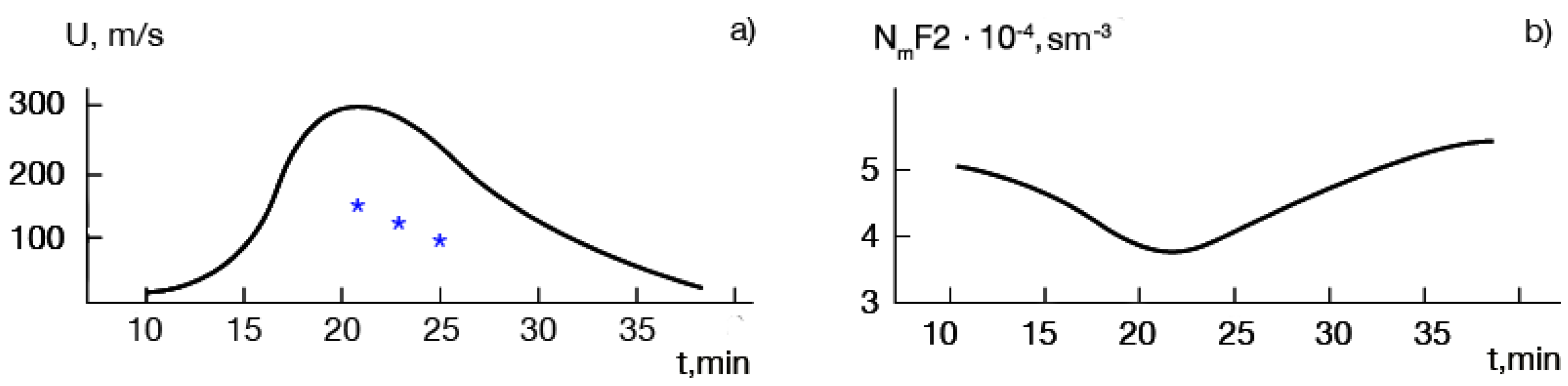
The ionosphere effect, a variation of electron concentration as a function of the vertical coordinate and time, is determined by the vertical component of velocity V(z,t). The plots of the velocity and electron density perturbation launched by the acoustic pulse are shown in Figure 3.

6. Discussion: Comparison

Due to the exponential growth of the amplitude with increasing altitude above sea level, even small disturbances (for example, for speeds of the order of 25 cm/s) at sea level increase at the altitudes of the ionosphere, which gives a gas velocity amplitude over 200 m/s, cf. [11]. This guarantees the possibility to use the model in tsunami diagnostics and the eventual prognosis of the wave impact at the seashore.

It is impossible to compare the results of our modeling and others’ directly because for such a situation, both models should have close mathematical statements of the problem and similar outputs. Some important features of the results, however, may be disclosed. Most closed problems were considered in the paper [13], where infra-sound propagation was studied. This is also the case in our work. The vertical profiles of the velocity for three moments of time given in Figure 11 of [13] allow estimating the amplitude at heights of about 300 km. We put the values in Figure 3a as stars. It is difficult to give a more detailed comparison between our results, due to the mentioned reasons. The order of amplitudes, at least, is the same.

Another important possibility is in comparison with the pulse arrival times $(t_a)$ at a prescribed height, estimated by the summation of the times $t_n=(h_n-h_{n-1})/v_{gn}$ ($v_{gn}$, the group velocity in n-layer). This was supported by information about the measurements in the paper [11]. More precisely, the arrival time was estimated by the condition ${\omega }_{dom}\approx {\omega }_c$ and evaluation of the time delay via the layer group velocities $t_i=1/k^{\prime }({\omega }_{dom,i})$. For the height of 100 km, it gives the value $t_a=t_1+t_2+t_3+t_4=319$ s, the sum of time delays for the first layers, which approximately corresponds to the result of the simulations and experiments given in [11].

The third one is related to ionosphere perturbations; see again [13]. The simulations show the variation of the electron density at the F-layer of about 8–10% (Figure 10 of [13]), which is in rather good correspondence with our estimations shown in Figure 3b. The lesser infra-sound wave amplitudes, shown in Figure 3a, left, produce lesser electron variations against ours, that is about 20%.

7. Conclusions

The main result of this paper is the recurrent formula that connects the exponentially-stratified adjacent layers of a planetary atmosphere. It allows constructing an algorithm for the solution of an acoustic wave propagation problem, starting with the appropriate time-dependent boundary condition at the planetary surface. The crucial element of this model is the projection procedure, derived for the z-evolution operator for the interface of layers. Such a procedure eliminates the down-directed wave and properly establishes the transition from the “n” layer to the next one “n + 1”. The model is applied to the problem of an acoustic wave initiated by a long ocean wave. The choice of the boundary regime is made on the basis of empirical data analysis. A model of the acoustic wave generated by the earthquake may be built in a similar fashion. The asymptotic expression of the resulting integrals by the large parameter (z) gives an explicit expression for the fluid velocity field at arbitrary heights in the frame of the proposed model. In return, it allows employing the explicit formula for the electron concentration at ionosphere layers.

Finally, combining the analytical formulas creates the basis for the algorithm that can evaluate the ionospheric effect very quickly. Such a model for tsunami or earthquake diagnostics may be beneficial.

An important step towards greater sophistication of the proposed 1D model would be to refine the boundary regime more appropriately to represent the tsunami wave. For instance, in [20,28], function (29), multiplied by a trigonometric function, was proposed. Such a modification allows computing the Fourier image and adjusting the working formula (34). The work will continue with the calculation of the ionospheric effect at altitudes above the second layer, given that the formalism is transferred to the next layer almost automatically.

References

- Hickey, M.; Schubert, G.; Walterscheid, R.L. Propagation of tsunami-driven gravity waves into the thermosphere and ionospher. J. Geophys. Res. 2009, 114. [Google Scholar] [CrossRef]
- Qingyun, Y.; Weimin, H. Tsunami detection and parameter estimation from GNSS-R delay-doppler map. IEEE J. Sel. Top. Appl. Earth Obs. Remote. Sens. 2016, 9, 4650–4659. [Google Scholar]
- Godin, O.A. Air-sea interaction and feasibility of tsunami detection in the open ocean. J. Geophys. Res. 2004, 109, C05002. [Google Scholar] [CrossRef]
- Zabotin, N.; Godin, O.; Bullett, T. Oceans are a major source of waves in the thermosphere. J. Geophys. Res. Space Phys. 2016, 121, 3452–3463. [Google Scholar] [CrossRef]
- Hines, C.O. Gravity waves in the atmosphere. Nature 1972, 239, 73–78. [Google Scholar] [CrossRef]
- Karpov, I.V.; Leble, S.B. The analytical theory of ionospheric IW effect in F2 layer. Geomagn. Aeron. 1986, 26, 234–237. (In Russian) [Google Scholar]
- Leble, S.B. Theory of Thermospheric Waves and their Ionospheric Effects. PAGEOPH 1988, 127, 491–527. [Google Scholar] [CrossRef]
- Rakoto, V.; Lognonne, P.; Rolland, L. Tsunami modeling with solid Earth-ocean-atmosphere coupled normal modes. Geophys. J. Int. 2017, 211, 1119–1138. [Google Scholar] [CrossRef]
- Kherani, E.A.; Lognonne, P.; Hebert, H.; Rolland, L.; Astafyeva, E.; Occhipinti, G.; Coisson, P.; Walwer, D.; de Paula, E.R. Modelling of the total electronic content and magnetic field anomalies generated by the 2011 tohokuoki tsunami and associated acoustic-gravity waves. Geophys. J. Int. 2012, 191, 1049–1066. [Google Scholar] [CrossRef]
- Peltier, W.R.; Hines, C.O. On the possible detection of tsunamis by a monitoring of the ionosphere. J. Geophys. Res. 1976, 81, 1995–2000. [Google Scholar] [CrossRef]
- Wei, C.; Buhler, O.; Tabak, E.G. Evolution of tsunami-induced internal acoustic–gravity waves. J. Atmos. Sci. 2015, 72, 2303–2317. [Google Scholar] [CrossRef]
- Wu, Y.; Llewellyn Smith, S.; Rottman, J.; Broutman, D.; Minster, J. The propagation of tsunami-generated acoustic–gravity waves in the atmosphere. J. Atmos. Sci. 2016, 73, 3025–3036. [Google Scholar] [CrossRef]
- Zettergren, M.D.; Snively, J.B. Ionospheric response to infrasonic- acoustic waves generated by natural hazard events. J. Geophys. Res. Space Phys. 2015, 120, 8002–8024. [Google Scholar] [CrossRef]
- Ma, J. Atmospheric Layers in Response to the Propagationof Gravity Waves under Nonisothermal, Wind-shear, and Dissipative Conditions. J. Mar. Sci. Eng. 2016, 4, 25. [Google Scholar] [CrossRef]
- Occhipinti, G.; Kherani, E.; Lognonne, A.; Geomagnetic, P. Three-dimensional waveform modeling of ionospheric signature induced by the 2004 Sumatra tsunami. Geophys. Res. Lett. 2006, 33. [Google Scholar] [CrossRef] [Green Version]
- Hines, C.O. Propagation velocities and speeds in ionospheric waves: A review. J. Atmos. Sol. Terr. Phys. 1974, 36, 1179–1204. [Google Scholar] [CrossRef]
- Holton, J.R. An Introduction to Dynamic Meteorology, 4th ed.; Academic Press: London, UK, 2004; 535p. [Google Scholar]
- Babich, V.M.; Buldyrev, V.S.; Kuester, E.F. Short-Wavelength Diffraction Theory: Asymptotic Methods; Springer: Berlin, Germany, 1991. [Google Scholar]
- Brekhovskikh, L.M.; Godin, O.A. Vol. 1: Plane and quasi-plane waves. In Acoustics of Layered Media; Springer: Heidelberg/Berlin, Germany, 1991. [Google Scholar]
- Leble, S.; Perelomova, A. Problem of proper decomposition and initialization of acoustic and entropy modes in a gas affected by the mass force. Appl. Math. Model. 2013, 13, 629–635. [Google Scholar] [CrossRef]
- Perelomova, A. Nonlinear dynamics of vertically propagating acoustic waves in a stratified atmosphere. Acta Acust. United Acust. 1998, 84, 1002–1006. [Google Scholar]
- Leble, S. General remarks on dynamic projection method. TASK Q. 2016, 20, 113–130. [Google Scholar]
- Leble, S. Reaction of Ionosphere Plasma to a Passing Internal Wave. In Nonlinear Waves in Waveguides with Stratification; Springer: Heidelberg/Berlin, Germany, 1990. [Google Scholar]
- Pelinovskiy, E.N. Hydrodynamics of Tsunami Waves; IPF RAN: Nizhny Novgorod, Russia, 1996; p. 276. [Google Scholar]
- Kurdyaeva, Y.A.; Kshevetskii, S.P.; Gavrilov, N.M.; Kulichkov, S.N. Correct Boundary Conditions for the High-Resolution Model of Nonlinear Acoustic-Gravity Waves Forced by Atmospheric Pressure Variations. Pure Appl. Geophys. 2018, 175, 3639–3652. [Google Scholar] [CrossRef]
- Kshevetskii, S.P. Theory and numerical modeling of the propagation and destruction of internal gravitational waves in the atmosphere. Kaliningrad State University: Kaliningrad, Russia, 2003. (In Russian) [Google Scholar]
- Karpov, I.V.; Leble, S.B. Solution of nonstationary problem of ionospheric response to a thermospheric disturbance. IZv. VUZ Radiophysica XX 1983, 1, 1599–1601. (In Russian) [Google Scholar]
- Dobrokhotov, S.Y.; Minenkov, D.S.; Nazaikinskii, V.E.; Tirozzi, B. Functions of noncommuting operators in an asymptotic problem for a 2D wave equation with variable velocity and localized right-hand side. Oper. Theory Adv. Appl. 2013, 228, 95–126. [Google Scholar]
Figure 1.
Multi-layered atmosphere model.
Figure 2.
This figure is the log–log plot of velocity solution illustration. is depicted at a height of = 10,000 m, the boundary between the first and the second layer. is depicted at a height of = 90,000 m, the boundary between the third and the fourth layer, = 7390 m, the average scale height in the first layer, and = 24,190 m, the average scale height in the fourth layer. For the parameter , we take 1/s [24].
Figure 3.
(a) Wave disturbance at a height of , the ionosphere layer maximum (the stars mark the results of [13]). (b) Variation in the ionosphere during the passage of a disturbance.
© 2019 by the authors. Licensee MDPI, Basel, Switzerland. This article is an open access article distributed under the terms and conditions of the Creative Commons Attribution (CC BY) license (http://creativecommons.org/licenses/by/4.0/).
Share and Cite
MDPI and ACS Style
Leble, S.; Smirnova, E. Tsunami-Launched Acoustic Wave in the Layered Atmosphere: Explicit Formulas Including Electron Density Disturbances. Atmosphere 2019, 10, 629. https://0-doi-org.brum.beds.ac.uk/10.3390/atmos10100629
AMA Style
Leble S, Smirnova E. Tsunami-Launched Acoustic Wave in the Layered Atmosphere: Explicit Formulas Including Electron Density Disturbances. Atmosphere. 2019; 10(10):629. https://0-doi-org.brum.beds.ac.uk/10.3390/atmos10100629
Chicago/Turabian StyleLeble, Sergey, and Ekaterina Smirnova. 2019. "Tsunami-Launched Acoustic Wave in the Layered Atmosphere: Explicit Formulas Including Electron Density Disturbances" Atmosphere 10, no. 10: 629. https://0-doi-org.brum.beds.ac.uk/10.3390/atmos10100629
Note that from the first issue of 2016, this journal uses article numbers instead of page numbers. See further details here.