The Contribution Rate of Driving Factors and Their Interactions to Temperature in the Yangtze River Delta Region


1
Faculty of Culture and Tourism, Shanxi University of Finance and Economics, Taiyuan 030006, China
2
Key Laboratory of Geographic Information Science (Ministry of Education), East China Normal University, Shanghai 200241, China
3
Research Center for East–West Cooperation in China, East China Normal University, Shanghai 200241, China
4
School of Geographic Sciences, East China Normal University, Shanghai 200241, China
5
Key Research Institute of Yellow River Civilization and Sustainable Development, Henan University, Kaifeng 475004, China
*
Authors to whom correspondence should be addressed.
Atmosphere 2020, 11(1), 32; https://0-doi-org.brum.beds.ac.uk/10.3390/atmos11010032
Submission received: 6 November 2019
/
Revised: 22 December 2019
/
Accepted: 24 December 2019
/
Published: 27 December 2019
(This article belongs to the Special Issue Climate Change, Climatic Extremes, and Human Societies in the Past)
Abstract
:Complex temperature processes are the coupling results of natural and human processes, but few studies focused on the interactive effects between natural and human systems. Based on the dataset for temperature during the period of 1980–2012, we analyzed the complexity of temperature by using the Correlation Dimension (CD) method. Then, we used the Geogdetector method to examine the effects of factors and their interactions on the temperature process in the Yangtze River Delta (YRD). The main conclusions are as follows: (1) the temperature rose 1.53 °C; and, among the dense areas of population and urban, the temperature rose the fastest. (2) The temperature process was more complicated in the sparse areas of population and urban than in the dense areas of population and urban. (3) The complexity of temperature dynamics increased along with the increase of temporal scale. To describe the temperature dynamic, at least two independent variables were needed at a daily scale, but at least three independent variables were needed at seasonal and annual scales. (4) Each driving factor did not work alone, but interacted with each other and had an enhanced effect on temperature. In addition, the interaction between economic activity and urban density had the largest influence on temperature.
1. Introduction
The climate system is a complex system, which influence on ecosystems and human society has attracted more and more attention from scholars, and temperature is one of the most important factors in the climate system.
A number of studies [1,2,3,4,5,6,7] have indicated that the spatiotemporal variation of temperature and its driving factors had regional differences. Sharma et al. [8] analyzed the temperature changes in eastern India, and the results showed that the average temperature in central, southern and western was decreasing, while the average temperature in the northeast, west and southeast was on the rise. Salman et al. [9] conducted a hybrid model to select the climate models for simulating spatiotemporal changes in temperature of Iraq. They found that temperature would increase during the period of 2070–2099 and temperatures in the north and northeast had increased significantly. Kenawy et al. [10] pointed out that temperatures in northeastern Spain showed an upward trend during the 1960–2006 period, and the Eastern Atlantic (EA), the Scandinavian (SCA), and the Western Mediterranean Oscillation (WeMO) patterns had a significant impact on temperature changes. Iqbal et al. [11] found temperature had different correlations with North Atlantic Oscillation (NAO), Arctic Oscillation (AO), El Niño-Southern Oscillation (ENSO), and North Sea Caspian Pattern (NCP) in different months in Pakistan. It can be seen that the temperature change is complicated. Therefore, further understanding the mechanisms for spatio-temporal variation of temperature and its driving factors are highly desired.
In order to reveal the complexity of temperature, many methods had been proposed, such as wavelet analysis [12,13], ensemble experience mode decomposition [14], spectrum analysis [15], Mann-Kendall trend test [16], and correlation dimension [17]. All of these methods had explored the complexity of temperature from different perspectives and got some achievements. On the other hand, there are many studies about the driving factors of temperature change. The main driving factors are atmospheric circulation [2], land use changes [3], greenhouse gas emissions [18], urbanization development [19], and so on. However, under the global warming, coupled with rapid economic development, population growth, and urbanization, the temperature and its driving factors became more and more complicated. In addition, the contribution rate of natural and socioeconomic factors and their interactions on temperature variation were rarely studied and remained one of main gaps in our current knowledge.
Due to the regional differences, it is necessary to conduct an in-depth analysis of temperature variations in some key areas, especially those that play an important role in national development. The Yangtze River Delta (YRD), one of China’s most developed, dynamic, densely populated and concentrated industrial areas, is growing into an influential world-class metropolitan area. However, the developed industries and frequent human activities have led to an increasingly serious urban heat island phenomenon in this region, forming a strong regional heat island, leading to the temperature presenting a significant warming trend over the past 50 years and extremely high temperatures occuring frequently [20]. Property, economic losses, and social impacts caused by extremely temperature events in this region are often enormous. In addition, extreme changes in temperature can also have an impact on the environment and endanger human health [21]. Therefore, it is of great significance to study the temperature changes in this region, to find the reasons that affect its changes, and to try to reduce losses.
Therefore, we attempt to explore the spatiotemporal dynamics of temperature in the YRD, and assess the influences of factors and their interactions on temperature. Based on observed temperature data at 68 meteorological stations during the period of 1980–2012, we first investigated the spatiotemporal complexity of temperature by using the Correlation Dimension (CD) method; and then we analyzed the individual contribution rates and interactional contribution rates of driving factors to temperature slope (TS) by using the Geogdetector method. Our main purpose is to explore which factors or interactions between factors contribute the most to temperature.
2. Materials and Methods
2.1. Study Area and Data
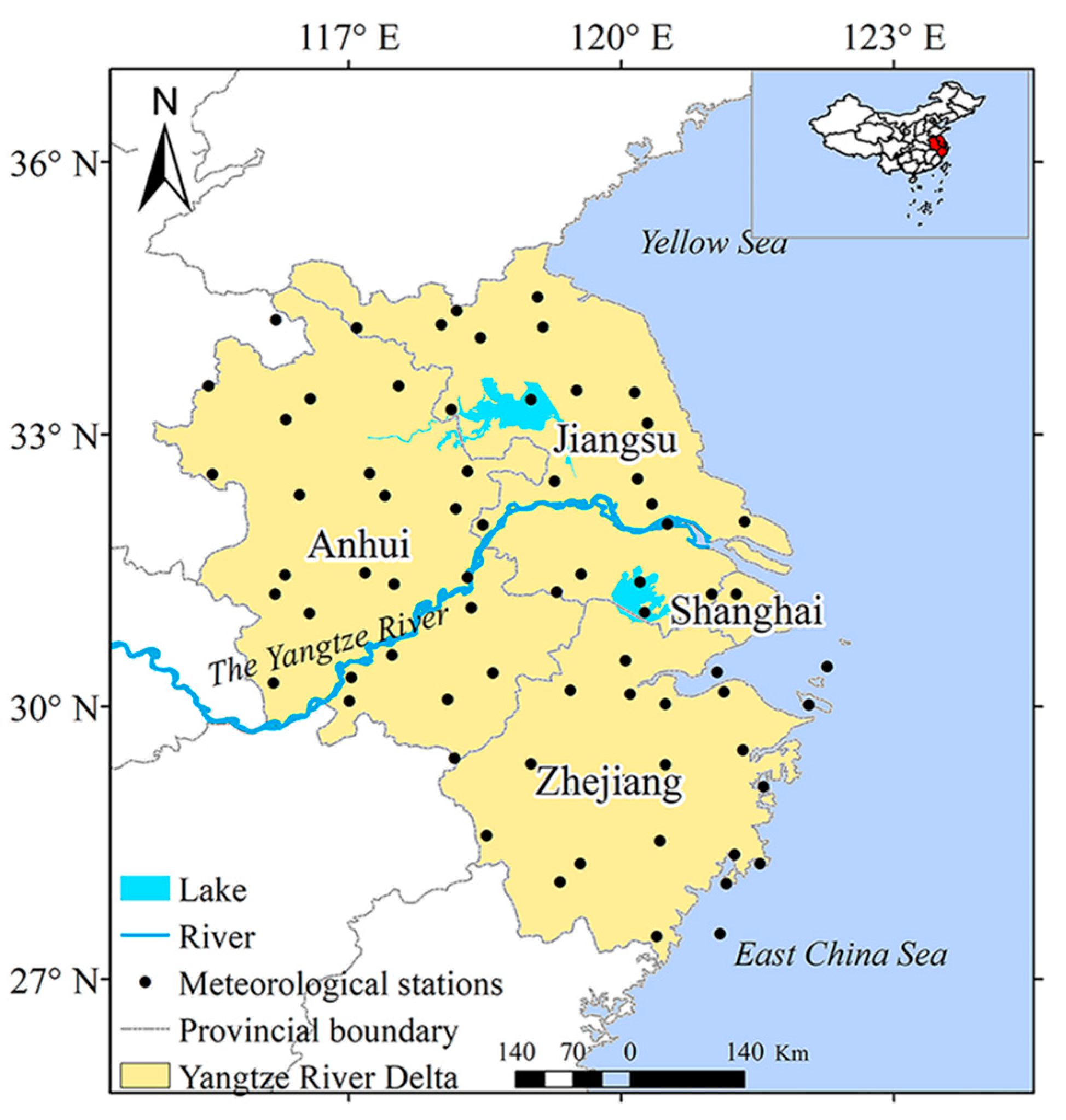
The study area includes four regions: Jiangsu Province, Anhui Province, Zhejiang Province, and Shanghai (Figure 1). The study area lies between 114°54′–122°42′ E and 27°12′–35°20′ N, and has an area of approximately 344.03 103 km2, accounting for 3.58% of China’s total land area. The area is under a monsoon climate regime, with hot and humid summer and cold and dry winter. The annual precipitation is about 1000 mm, of which the precipitation in summer accounts for two-thirds of the total precipitation [22]. The average temperature is close to 30 °C in July and August, and the maximum temperature recently exceeded 40 °C in Shanghai [23]. The high terrain is in the north and south and low terrain in the middle, which is dominated by plains and hills. In addition, the YRD is one of the most developed regions in China, with dense population, convenient transportation, and developed tertiary industry.
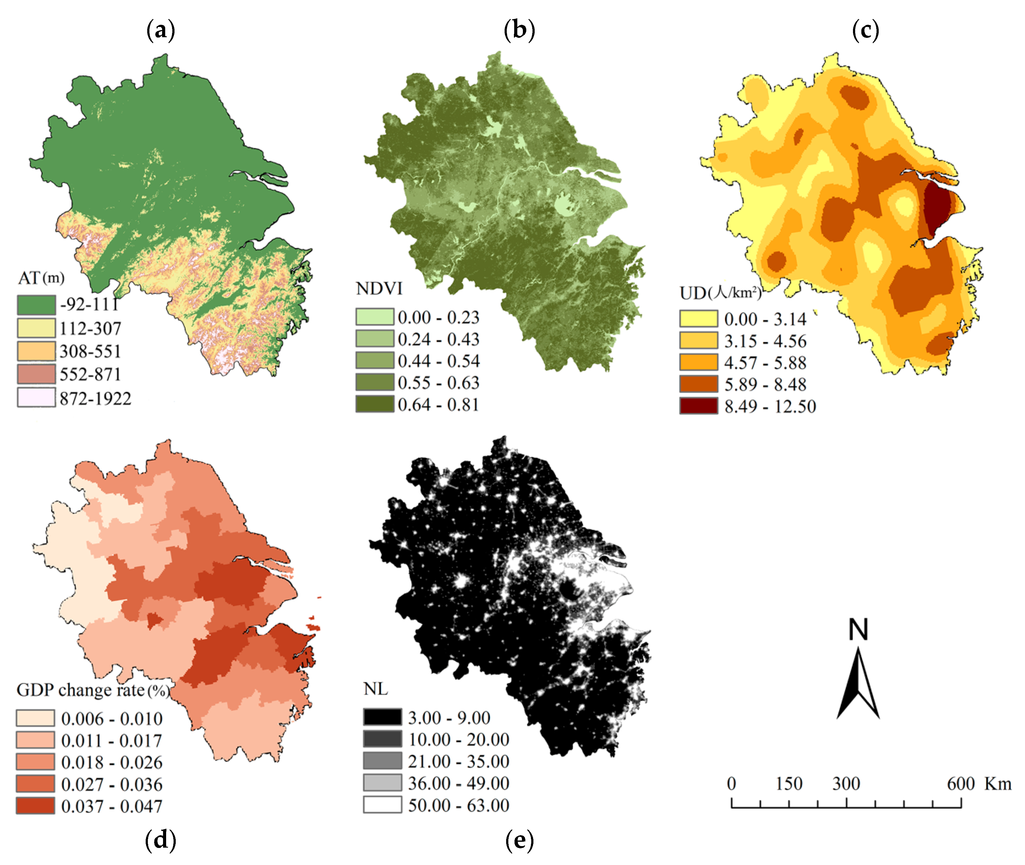
On a global scale, the temperature is mainly affected by factors such as atmospheric circulation, volcanic eruptions, sunspots, and so on. However, on the regional scale, the temperature is mainly affected by surface properties and human activities. According to previous studies [24,25,26], the altitude (AT), normalized difference vegetation index (NDVI), urban density (UD), gross domestic product (GDP), and night light (NL) datasets were selected. The first two can be seen as natural factors and the last three can be seen as socioeconomic factors. The daily temperature of 68 meteorological stations from 1980 to 2012 is from the China Meteorological Data Service Center (http://data.cma.com). We analyzed data from the period from 1980 to 2012 because we couldn’t get station data of temperature for 2013–2018. AT and UD data are provided by the Data Center for Resources and Environmental Sciences, Chinese Academy of Sciences (RESDC) (http://www.resdc.cn), and the UD data is from 1990 to 2010. NDVI is from the Geospatial data cloud (http://www.gscloud.cn/), and its period is from 1989 to 2012. NL is from the National Centers for Environmental Information (https://www.ngdc.noaa.gov/), and its period is from 1992 to 2012. GDP is from the “Shanghai Statistical Yearbook”, “Anhui Statistical Yearbook”, “Jiangsu Statistical Yearbook”, “Zhejiang Statistical Yearbook”, and “China Regional Economic Statistics Yearbook” and other statistics, and its period is from 1980–2012. To ensure a consistent data format, a 0.5 km by 0.5 km grid for the whole area in ArcGIS 10.5 software (Manufacturer, City, US State abbrev. if applicable, Country) was built, assigned values to each grid, and deleted the outliers by using a box-plot analysis method. According to different standards, all factors were divided into different strata using ArcGIS 10.5 software. The division of the results is shown in Figure 2 below.
2.2. Methods
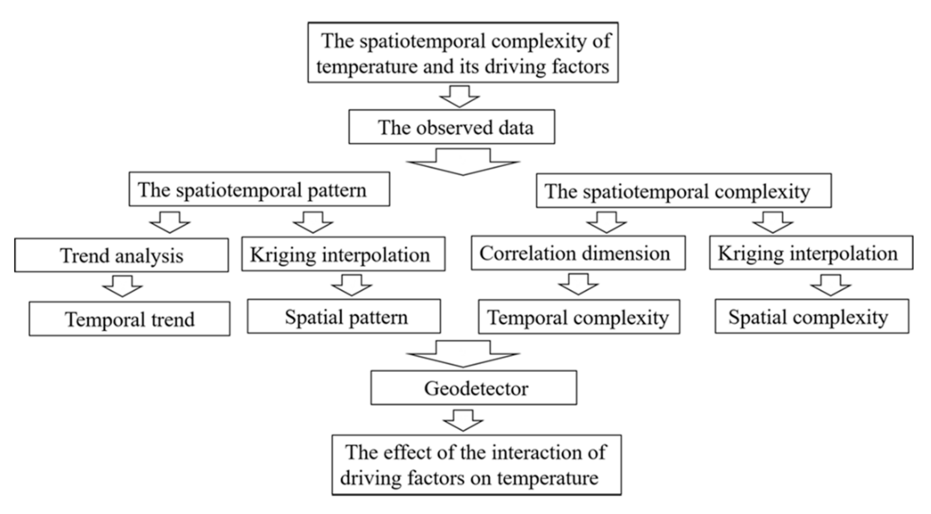
To investigate the spatiotemporal complexity of temperature and its driving factors, the correlation dimension method and the Geogdetector method were used. It can be seen from Figure 3, we first showed the spatiotemporal pattern of temperature; then, we analyzed the complexity of temperature on the daily, seasonal, and annual scales by using the Correlation Dimension (CD) method;finally, the individual contribution rates and interactional contribution rates of driving factors to the temperature slope (TS) by using Geogdetector method were detected.
2.2.1. Trend Analysis Method
Trend analysis is the most studied and most popular quantitative forecasting method by far. It is based on a known historical data to fit a curve, so that this curve can reflect the growth trend of things themselves, and then to predict the future according to this growth trend curve. Commonly used trend models include linear trend models, polynomial trend models, linear trend models, log trend models, power function trend models, exponential trend models, and so on [27]. In this study, we use the linear trend method to analyze the change trend of the time series:
where y represents the time series, t represents the time, a represents the linear slope, and b represents the intercept.
If a > 0, it indicates that the time series is increasing, if a = 0, it means that the time series is not changing, and, if a < 0, it indicates that the time series is decreasing. The size of a indicates the degree of change in time series.
2.2.2. Kriging Interpolation Method
Temperature is a regionalized variable, which is changing with the variation of space position. In order to analyze the distribution of the plum rainfall in different years, Kriging interpolation is employed. Kriging interpolation (or space local estimation) is named by D. G. Krige, who is a mining engineer in South Africa, and it is an optimal interpolation method [28]. The original data of the regional variables and the structural characteristics of the variance function is used to estimate the value of non-sampling points unbiasedly and optimally [28]. In general, Kriging interpolation contains several types, namely Ordinary Kriging, Universal Kriging, Co-Kriging, and so on. Ordinary Kriging is shown below:
Assume that is a regionalized variable that satisfies two-stage stationary hypotheses and intrinsic hypothesis. m is mathematical expectation, with covariance function and variance function all existing at the same time. The relation between them is indicated below:
Assuming that there are no measured points in the neighborhood of x, namely , for which the sample value is , the formula can be defined as follows:
where is a weight coefficient that presents the contribution degree of the observed values of to estimate the values of . Two points need to be noticed about this formula: on the one hand, the estimated value of must be unbiased, namely the mathematical expectation of the deviation is zero; on the other hand, it must be optimal, namely the difference between the estimated value and the actual value is the smallest.
2.2.3. Correlation Dimension (CD)
Since the appearance of fractal theory, fractal dimension has been welcomed by scholars as one of the quantitative indicators to describe whether the dynamic system has chaotic characteristics. There are different types of fractal dimensions, such as topological dimension, Hausdorff dimension, information dimension, and correlation dimension. As for the correlation dimension, Grassberger and Procaccia [29] proposed an analysis method for experimental time series data in 1983, which is to obtain the fractal dimension through the relationship between the integral C (r) and the distance r on the reconstructed phase space through the univariate time series. This method is called a G–P method. Because it is particularly suitable for experimental observation data and the algorithm is simple and easy to implement, it has been widely used. In this study, we use this method when calculating the correlation dimension.
The correlation dimension (CD) is usually applied to analyze time series and determine if it exhibits a chaotic dynamic characteristic [30,31]. Considering {x1, x2, x3, …, xi, …}, the equal interval time series of daily temperature, and the first m data are extracted, and they determine the first point in the m-dimensional space, which is denoted as X1. Then, remove x1, and take m data x2, x3, …, xm+1, and the second point is composed of this set of data in m-dimensional space, which is recorded as X2. According to this, a series of phase points X1, X2, …, XN are formed. Given the number r, and check how many point pairs (Xi, Xj) distance is less than r, and the ratio of the number that point pairs distance is less than r to the total number of point pairs N is denoted as C(r) [17]. It can be expressed as the following formula:
where θ(x) is the Heaviside function, which is defined as:
If r is too large, the distance of all point pairs will not exceed it. In addition, this r cannot measure the correlation between phase points. In addition, appropriate reduce r, the following formula may exist:
If this relationship exists, d is a dimension called the correlation dimension, denoted as D2:
The limit here mainly represents a direction in which r is reduced, and it is not mean that the r must be close to 0. In the scale transformation of the actual system, there are scale restrictions in the magnitude of both directions. Exceeding this limit is beyond the featureless scale area.
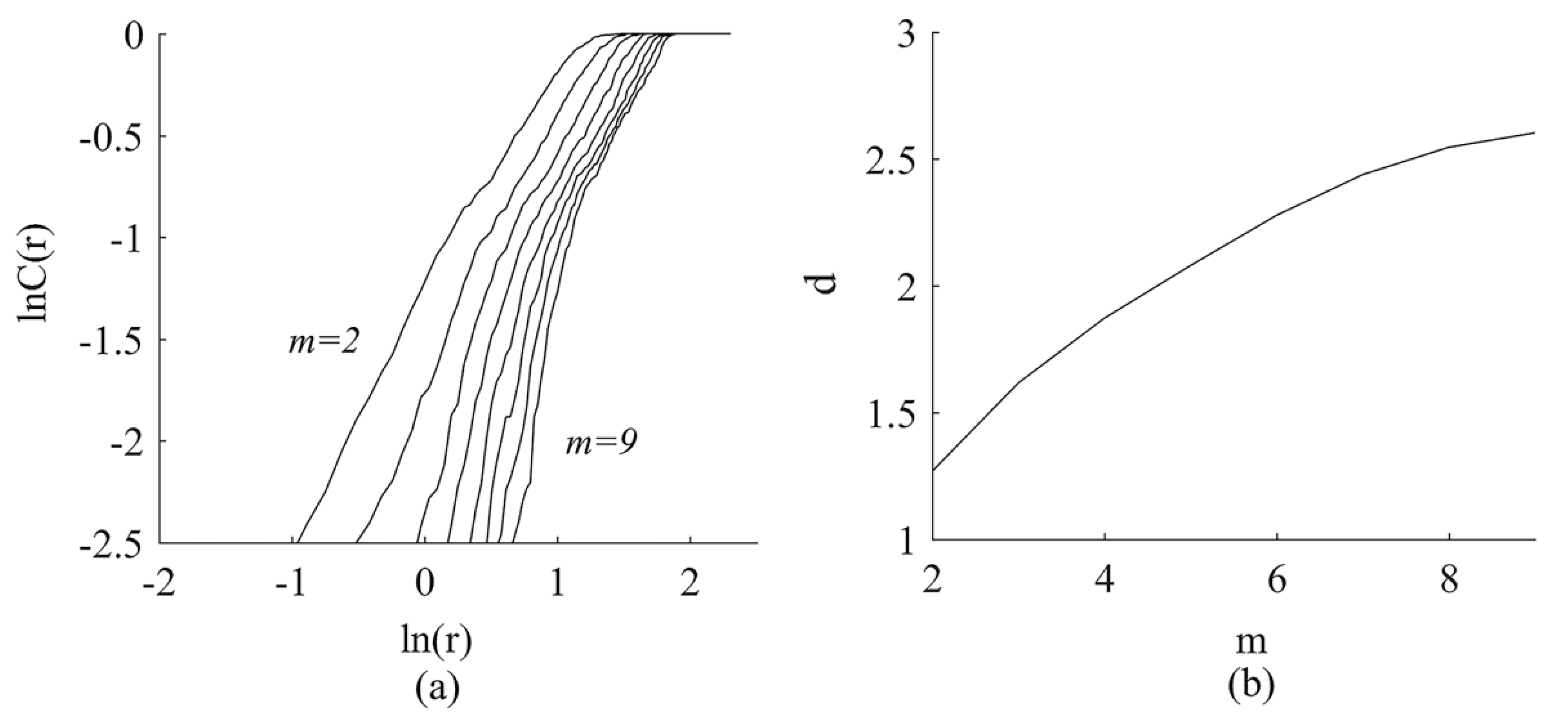
Figure 4 shows the results of ln(r) versus ln(r), and the correlation dimension (d) versus embedding dimension (m) used the measured data of temperature in this paper. It is apparent that the correlation dimension, D2, is given by the slope coefficient of ln(r) versus lnr. According to (lnr, lnC(r)), D2 can be obtained by the least squares method using a log–log grid (as shown in Figure 4a).
To detect the chaotic behavior of the system, the correlation dimension has to be plotted as a function of the embedding dimension (as shown in Figure 4b).
The MATLAB 2014a software (Manufacturer, City, US State abbrev. if applicable, Country) was used to calculate Correlation Dimension. First, we calculated the time series of daily average temperature, monthly average temperature, and annual average temperature of each meteorological station during the period of 1980–2012, and then calculated the CD value of each station on different time scales through programming using MATLAB software (The MathWorks, Natick, MA, USA).
2.2.4. Geogdetector
The influencing factors have spatial heterogeneity and work together to affect the temperature. Geogdetector is a set of statistical methods for detecting spatial variability and revealing forces driving the variability [32,33]. The advantages of this method are that it cannot only detect both quantitative and qualitative data, but also can detect the interaction of two factors [34]. Geogdetector contains four detectors: a risk detector, a factor detector, an ecological detector, and an interaction detector.
The risk detector can determine whether there is a significant difference in the means of attributes between two sub-regions, using the t statistic to test:
where is the attribution average in the region h, is the sample size of sub-region h, and Var is the variance. The statistic t approximates the Student’s distribution, where the degree of freedom (df) is calculated as:
Null hypothesis: . If H0 is rejected at significance level α, there is a significant difference in the mean of the attributes between the two sub-regions.
The factor detector mainly detects the spatial variability of Y and the extent to which X is probed to explain the spatial differentiation of Y. The q-value was used to measure the factors:
where h = 1, …, L is the stratum of Y or X, Nh, and N are the unit numbers of layer h and the unit numbers of the whole region, respectively, and and are the variances of Y of the layer h and of the whole region, respectively. SSW and SST are the sum of squares and the total sum of squares, respectively. The range of q is [0, 1]. The larger the value, the more obvious the spatial distribution of Y is. If the stratum is generated by the independent variable X, a larger q value shows stronger explanatory power of the independent variable X to Y, and a smaller q means weaker power. In extreme cases, a q value of 1 indicates that factor X has complete control over the spatial distribution of Y, and a q value of 0 indicates that factor X has no control over the spatial distribution of Y.
The ecological detector explores whether a geographical stratum, C, is more significant than another stratum, D, in controlling the spatial pattern, and the statistic F is used to measure it:
where Nx1 and Nx2 are the sample sizes of factors X1 and X2, respectively, and SSWx1 and SSWx2 are sums of the variances in the strata formed by X1 and X2, respectively. L1 and L2 represent the number of variables in X1 and X2, respectively. H0 is SSWx1 = SSWx2. If H0 is rejected at the significance level of α, there is a significant difference in the spatial distribution of Y between X1 and X2.
The interaction detector is used to evaluate whether X1 and X2 together will increase or decrease the explanatory power of the dependent variable Y, or whether the effects of these factors on Y are independent of each other. q(X1), q(X2), and q((X1∩X2) were calculated and compared the differences between q(X1), q(X2), and q((X1∩X2).
The Geogdetector software was used to calculate Geogdetector. First, we need to calculate the annual average of temperature, AT, NDVI, UD, GDP change rate, and NL in their respective time periods, and convert the data format to .tif format; secondly, a 0.5 × 0.5 km grid is established by ArcGIS software, and each variable is extracted by the points in the grid; next, the extracted AT, NDVI, UD, GDP change rate, and NL were classified respectively. In this study, these variables are divided into five categories according to the natural segmentation method in ArcGIS software. Finally, the processed data is imported into the Geogdetector software for calculation.
3. Results
3.1. The Spatiotemporal Pattern of Temperature
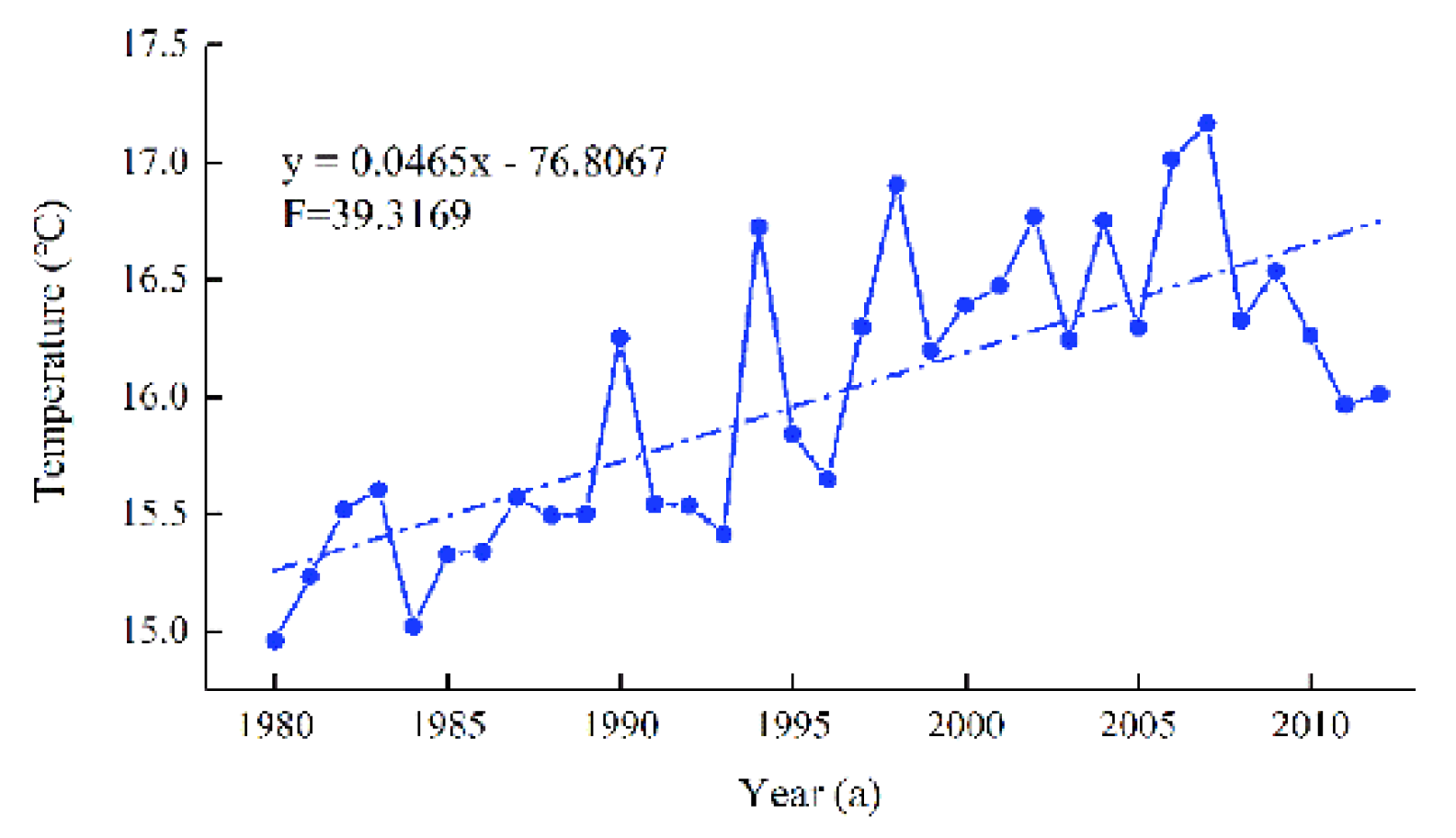
In order to understand the temperature variations during the period of 1980–2012 in the YRD, we first analyzed the overall trend of temperature variation by using the linear trend method, and the linear slope is used to identify the trend of temperature changes. If the linear slope is greater than 0, it indicates that temperature is increasing, if the linear slope is equal to 0, it means that temperature is not changing, and, if the linear slope is less than 0, it indicates that temperature is decreasing. It showed a significant increasing trend during the period of 1980–2012 (Figure 5), and this trend may continue in the future. We can see that the temperature rose 1.53 °C with the average rising rate of 0.465 °C/10 years and passed the significance test during the period of 1980–2012. However, in the most recent 50 years, the global average rising rate only has reached about 0.13 °C/10 years [35]. We can conclude that the increase in temperature in the YRD was not only the result of global warming, but also other regional factors.
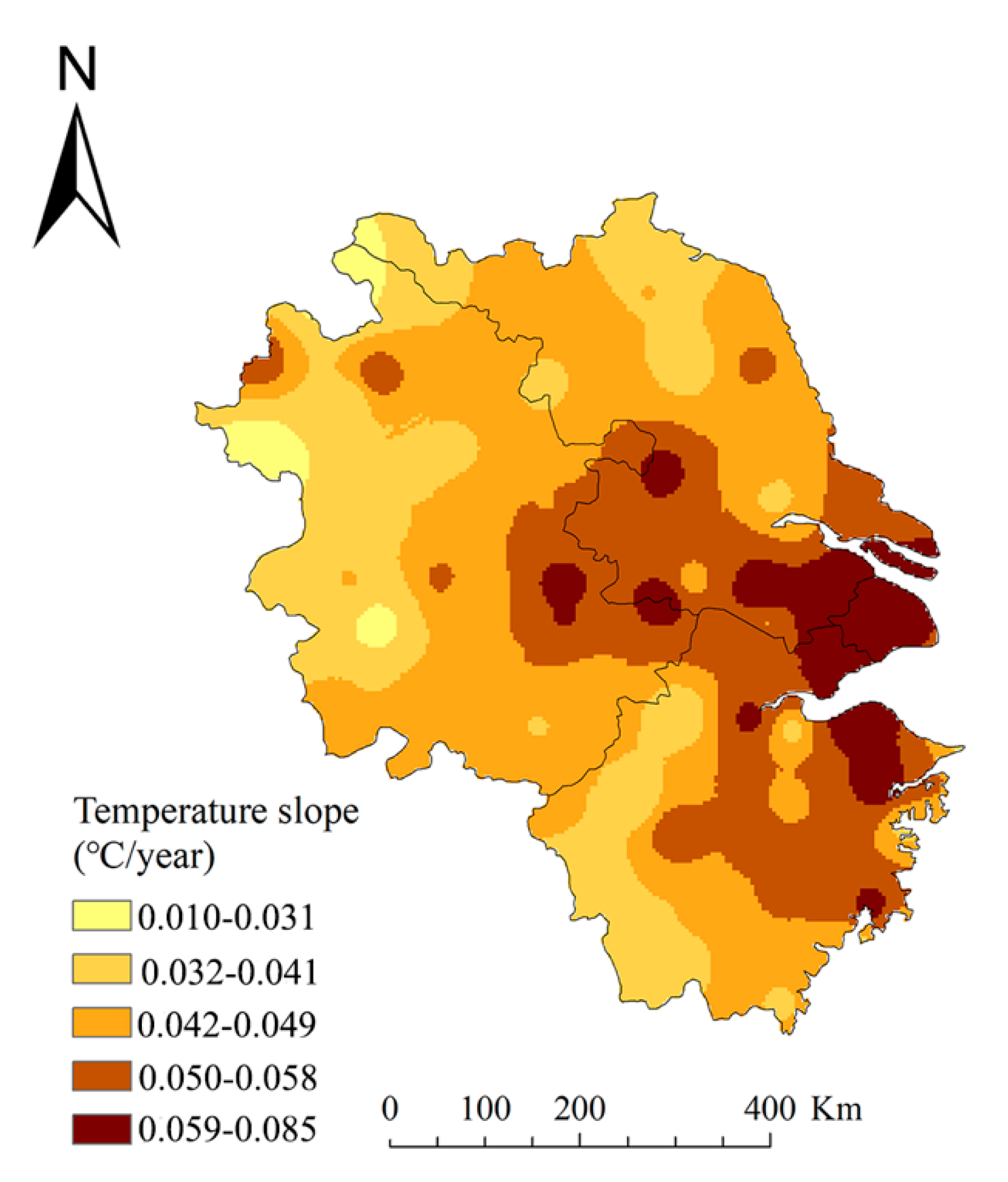
Then, we showed the spatial distribution of TS during the period of 1980–2012 (Figure 6). The ordinary Kriging method was used during the interpolation, in which a spherical model is used when selecting the semi-variogram model, and its parameters are system default parameters. We can see that the temperature rose in all regions. In addition, among the dense areas of population and urban, the temperature rose quickly, while the temperature in the sparse areas of population and urban rose slowly.
3.2. The Spatiotemporal Complexity of Temperature
3.2.1. The Temporal Complexity of Temperature
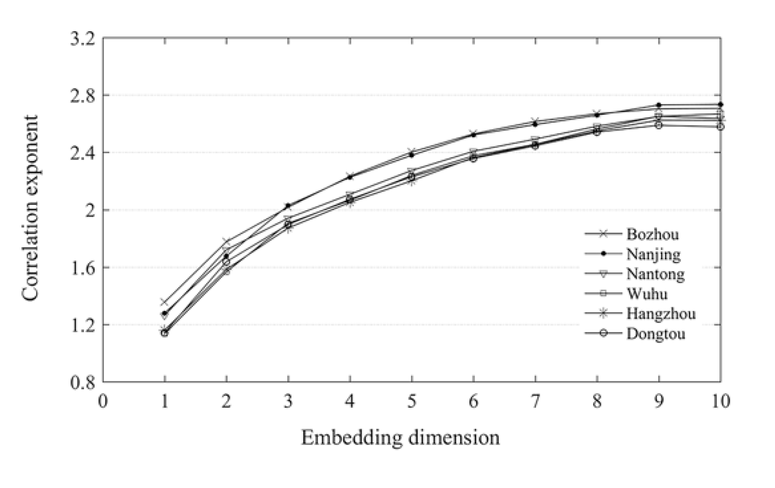
Based on meteorological data, we analyzed the chaotic dynamics with fractal characteristic for the temperature dynamics by using the G–P method [36]. Firstly, we randomly selected six meteorological stations (i.e., Bozhou, Nanjing, Nantong, Wuhu, Hangzhou, Dongtou) with annual time series data for a pilot study. The relationship between different embedding dimension (m) and correlation exponent (d) was shown in Figure 7.
It can be seen from the trend of the six meteorological stations in Figure 7 that, as the embedding dimension increases, the correlation exponent increases continuously and eventually stabilizes, and the saturated correlation exponent, namely, the correlation dimension, was obtained when m ≥ 10.
Then, we calculated the CD on the daily, seasonal and annual temporal scales of each station in the same way. Table 1 shows the CD values of several representative stations and average CD values of all stations at different temporal scales. It can be seen from Table 1 that each CD is not an integer, which indicates that the temperature process at different temporal scales is a chaotic dynamic system with a fractal characteristic, and it is sensitive to the changes of initial conditions.
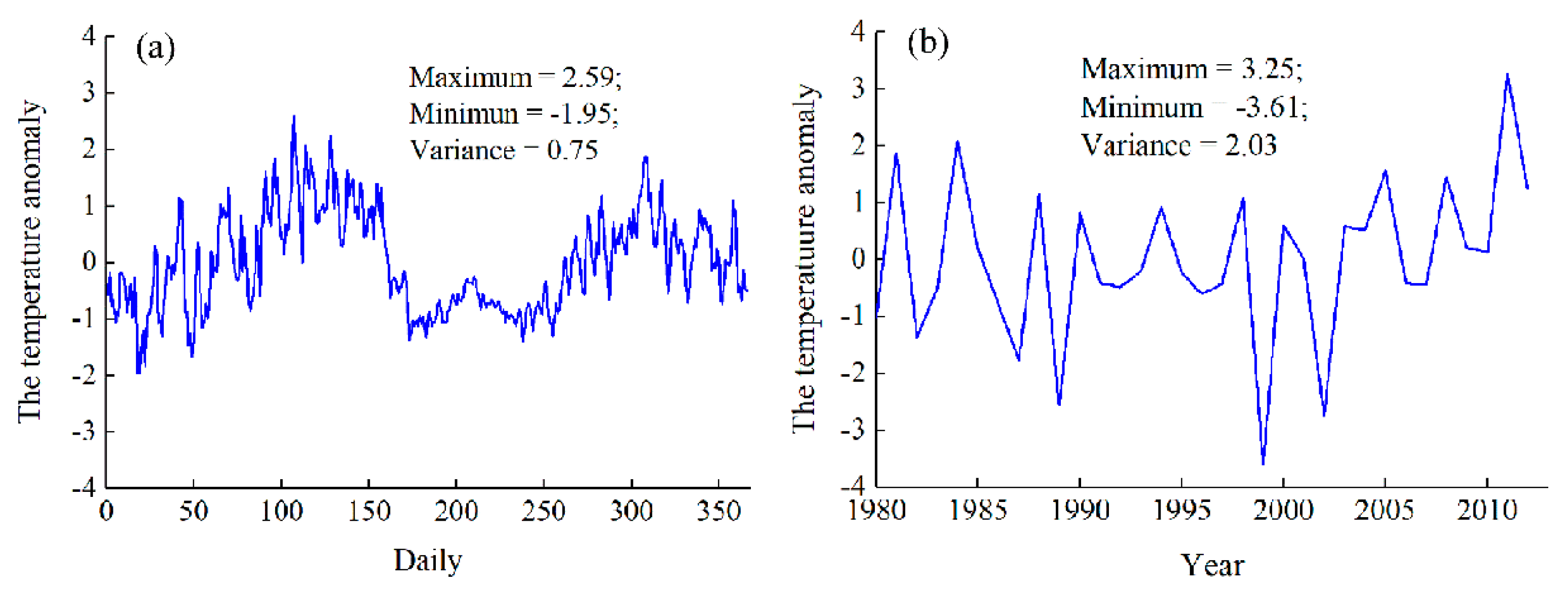
It can be seen from the mean of correlation dimensions (MCD) at different temporal scales in Table 1 that the ordering of the CD is: annual (2.32) > seasonal (2.08) > daily (1.73). We can conclude that the temperature process over a larger temporal scale is more complicated than the temperature process at a small temporal scale. Figure 8 showed the temperature anomalies of daily range and temperature anomalies of annual range. It could be seen from the maximum, minimum, and variance that the annual temperature fluctuated greatly, which proved that the temperature process on the annual scale was more complicated. Table 1 also shows that, even at the same temporal scale, the CD values of different stations are different. It is mainly related to the different locations of each station, which makes the driving factors of each station different. The values of MCD on the seasonal and annual scales are greater than 2, with 2.2 and 2.4, respectively, indicating that at least three independent variables are needed to describe the dynamics of temperature process on the seasonal and annual scale; and the value of MCD for daily is 1.73, indicating that at least two independent variables are needed to describe the dynamics of temperature process on the daily scale.
3.2.2. The Spatial Distribution Complexity of Temperature
Table 1 gives the CD values of the temperature on different temporal scales, showing temperature dynamics on the daily, seasonal and annual scales. What is the spatial distribution of the CD values of different stations? We show the spatial distribution of CD values on the daily, seasonal, and annual scales (Figure 9). The ordinary Kriging method was used during interpolation, in which a spherical model is used when selecting the semi-variogram model, and its parameters are system default parameters.
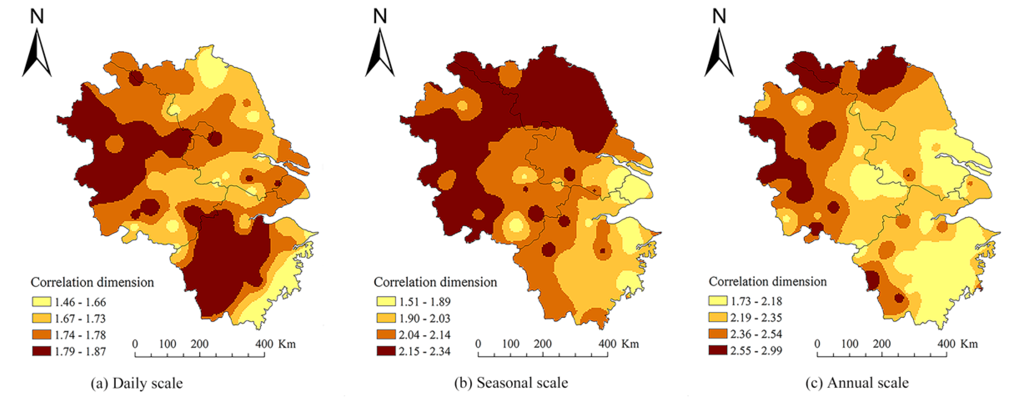
Figure 9a shows the spatial distribution of CD values on the daily scale, with values between 1.46 and 1.87. High value is mainly distributed in the northwest and southwest of the entire region, while low values are mainly distributed in the eastern coastal areas. Figure 9b presents the spatial distribution of CD values on the seasonal scale, which shows that all CD values are between 1.51 and 2.34. High value is mainly distributed in the northwest of the entire region, while low values are mainly distributed in the eastern coastal areas. Figure 9c shows the spatial distribution of CD values on the annual scale. All CD values are between 1.73 and 2.99, and the spatial pattern is similar with the spatial pattern on the seasonal scale. As we all know, the eastern coastal areas, especially Shanghai, Suzhou, and Hangzhou, are densely populated and have high levels of urbanization, and the CD value of this area is relatively low, while the areas located in the northwest of the YRD, such as Bozhou, Xuzhou, and Fuyang, the large outflow of people results in a relatively small population in these areas, and the urbanization level is relatively low, and the CD value in this area is relatively high. It can be seen that the population density and the urbanization level are related to CD.
In general, on different temporal scales, the high values of CD are mainly distributed in the sparse areas of population and urban, while the low values of CD are mainly distributed in the dense areas of population and urban.
3.2.3. The Influences of Driving Factors and Their Interactions on Temperature Slope
From the above results, we can see that the spatial distribution of TS is different, and what is the reason for this result? In order to answer this question, we choose some driving factors (AT, NDVI, UD, GDP, and NL) that affect the temperature to explore the reasons of this phenomenon by using the Geogdetector method.
The factor detector is used to detect whether the driving factors affect TS and the size of their influences. In addition, the greater the value of q, the greater the influence of this factor on TS. Table 2 shows the result of the factor detector. On the whole, the influence, in order of size, of each factor is: UD (0.323) > GDP (0.234) > NL (0.218) > NDVI (0.118) > AT (0.047). In addition, all driving factors pass the significant test, which means that these five factors have significant effects on TS. In addition, we can see that the contribution rate of socioeconomic factors (UD, GDP, NL) is greater than natural factors (NDVI, AT).
Whether the factor has a significant difference in the spatial distribution affecting the TS is achieved by an ecological detector. A test with a significance level of 0.05 indicates that the two factors are different influencing the distribution of TS; otherwise, there is no significant difference. The result of an ecological detector is shown in Table 3.
The result shows that there is a significant difference between UD and GDP; there is no significant difference between AT, NL, NDVI, and GDP, indicating that the effects of AT, NL, NDVI, and GDP on the spatial distribution of TS are similar. In addition, there is a significant difference between UD and NL, AT, and there is no significant difference between UD and NDVI. Similarly, there is a significant difference between NL and AT, while NL is not significantly different from NDVI. For AT and NDVI, there is also a significant difference between them. We can also conclude that the influences of various driving factors on the TS are different.
Table 2 indicates that the contribution rate of each factor alone to the TS is different. Thus, there is an interaction between them, and, if so, what is the interaction result? In order to answer this question, we give the results of interaction detector as Table 4.
Table 4 shows that only AT and GDP have a nonlinear enhancement effect (q (GDP∩ AT) > q(GDP) + q(AT)) on TS, and the interactions between remaining driving factors have the bi-enhancement effect on TS. It shows that the effect of interaction of any two factors is greater than the effect of a single factor. Among them, the interaction effect between GDP and UD (q (GDP ∩ UD) = 0.464) is the largest, and the interaction effect between UD and NL (q (UD∩ NL) = 0.420) is second, followed by the interaction effect between UD and NDVI (q (UD∩NDVI) = 0.393) and the interaction effect between GDP and NL (q (GDP∩ NL) = 0.391), while the interaction effect between AT and NDVI (q (AT∩NDVI) = 0.146) is the smallest. In general, the interaction effect between socioeconomic factors is the largest, the interaction effect between socioeconomic factors and natural factors is second, followed by the interaction effect between natural factors.
4. Discussion
In this study, we found that the temperature rose 1.53 °C with an average rising rate of 0.465 °C/10 years during the study period, which was higher than the global average rate. The result was consistent with previous studies [37,38,39]. It confirms the regional differences in climate change. In addition, it means that the temperature was not only affected by global warming, but also affected by various driving factors within the region. In addition, the temperature rose quickly in the dense areas of population and urban, and the temperature rose slowly in the sparse areas of population and urban. It reflected the urban-rural differences in temperature distribution from the side.
The climate system was an open system with external forcing and nonlinear dissipation [40], and fractal theory was one of the effective methods to quantitatively describe the nonlinear evolution process of climate and its self-similar structural features. Numerous studies [41,42,43,44,45] had shown that fractal analysis could calculate its fractal dimension from a seemingly chaotic climate sequence, confirming the fractal information of the climate system. Temperature was an element of the climate system and also had nonlinear characteristics. Especially in the YRD, the temperature was more complicated due to the influence of human activities. By calculating the CDs on the daily, seasonal, and annual scales of the YRD, we confirmed that the temperature in the YRD was a chaotic dynamic system with nonlinear characteristics. We found that temperature on the annual scale was more complicated than on the daily scale in the YRD. It was because the annual average temperature was the average of the daily temperature, which was the macroscopic performance of the daily temperature and influenced by many factors [46,47], so it showed greater complexity on the whole. Xu et al. [17] found that the temperature process on the daily scale was more complicated than the temperature process on the annual scale in Xinjiang. It was contrary to the YRD, indicating the complexity of the temperature process had regional differences. In the spatial distribution, whether in the daily, seasonal, or annual scale, the high CD values were mainly distributed in the sparse areas of population and urban, while the low CD values were mainly distributed in the dense areas of population and urban. In the dense areas of population and urban, due to the density of cities and people, industrial and urbanization were developing rapidly, and the temperature was mainly affected by the rapid development of cities, showing an upward trend [38]. While in the sparse areas of population and urban, the temperature changes were mainly affected by natural factors and socioeconomic factors together, so the temperature changes more complicated.
The effects of five driving factors on the TS were quantitatively investigated by using the Geogdetector method. UD was the most important factor affecting TS. From Figure 2c and Figure 8, we can see that the spatial distribution of UD was similar to the spatial distribution of TS, that is, decreasing toward the periphery with Shanghai as the center. The UD reflected the intensity of the city. In Shanghai and its surrounding areas, cities were dense and urbanization was high. One of the most striking features of this was that the impervious surface of the city increased rapidly [48,49]. The impervious surface of the city had strong heat storage, poor water storage capacity, and hindering airflow transmission, which seriously affected the city’s surface hydrological cycle [50], energy distribution [49] and urban microclimate [51], resulting in an urban heat island effect, which causes the temperature in dense areas of urban to rise quickly. The impact of urban impervious surface on surface temperature had been verified in different regions and a certain consensus had been reached [52,53,54,55]. The contribution rate of GDP to TS was second. From Figure 2 and Figure 6, we can see that the spatial distribution of GDP was similar to the spatial distribution of TS. The development of GDP inevitably consumed a large amount of energy, which would emit a large amount of greenhouse gases, resulting in a quick increase in temperature. The GDP in Shanghai and its surrounding areas was increasing rapidly, so the TS in this area was high. The contribution of NL was similar to the contribution rate of GDP, and the spatial distribution of NL was similar to the TS. NL reflected the level of GDP and energy consumption from the side [56,57], so it had a high contribution rate to TS. The NDVI was the smallest in Shanghai and its surrounding area, while the TS was largest in this area, which meant that the vegetation coverage rate played an important role in suppressing the increase of temperature, but it was not enough only to rely on the vegetation coverage rate. Most of the YRD was plain and the fluctuation of terrain was small, so the contribution rate of AT to the TS was small and can be ignored. Each driving factor had an effect on TS; they did not work alone, but different driving factors interacted with each other and had an enhanced influence on temperature.
Our main purpose is to explore which factors or interactions between factors contribute the most to temperature. The paper only analyzed the complexity of the temperature process and the contribution rates of driving factors to temperature, but the mechanism behind it remains to be studied further. In addition, through the analysis of the driving factors, some policy opinions to mitigate the temperature rise need to be proposed in the next study.
5. Conclusions
The study first analyzed the spatiotemporal variations of temperature in the YRD during the period of 1980–2012 by using the trend analysis method; then, we investigated the spatiotemporal complexity of temperature on different time scales by using the correlation dimension; finally, the effects of driving factors and their interactions on TS in the YRD during the period of 1980–2012 was analyzed by using the Geogdetector method. Summarizing this study, the main conclusions are as follows:
- The temperature was increasing during the period of 1980–2012, and it rose by 1.53 °C from 1980 to 2012; in addition, among the dense areas of population and urban, the temperature rose quickly, while the temperature in the sparse areas of population and urban rose slowly.
- In the temporal, the temperature process was more complicated with the increase of temporal scale; in the spatial distribution, whether it is the daily time scale, the seasonal time scale, or the annual time scale, the temperature process was more complicated in the sparse areas of population and urban than the dense areas of population and urban.
- Socioeconomic factors were the main factors affecting climate change in the YRD, and the contribution rate of urban density is the largest among the contribution rates of single factors. In addition, the interactions between various driving factors had an enhanced effect on regional climate change. In addition, the interaction between economic activity and urban density had the largest influence on temperature.
Author Contributions
C.Z. designed, carried out the analysis, and wrote the manuscript. N.Z. revised the paper and refined the results, conclusion, and abstract. D.Y. discussed the results. N.Z. edited the figures. J.X. revised the paper and gave the commentary. All authors have read and agreed to the published version of the manuscript.
Funding
This research was funded by the Scientific and Technological Innovation Programs of Higher Education Institutions in Shanxi, Grant No. 2019L0477 and the Humanities and Social Sciences Foundation of the Ministry of Education of China, Grant No. 19YJA890006.
Acknowledgments
The authors are grateful to the Resource and Environmental Science Data Center (http://www.resdc.cn) of the Chinese Academy of Sciences and the China Meteorological Data Sharing Service System (http://cdc.cma.gov.cn/) for providing data. The authors appreciate the insightful comments of anonymous reviewers.
Conflicts of Interest
The authors declare no conflict of interest.
References
- Wang, B.; Zhang, M.; Wei, S.; Wang, S.; Li, S.; Ma, Q.; Li, X.; Pan, S. Changes in extreme events of temperature and precipitation over Xinjiang, northwest China, during 1960–2009. Quatern. Int. 2013, 298, 141–151. [Google Scholar] [CrossRef]
- Horton, D.E.; Johnson, N.C.; Singh, D.; Swain, D.L.; Rajaratnam, B.; Diffenbaugh, N.S. Contribution of changes in atmospheric circulation patterns to extreme temperature trends. Nature 2015, 522, 465–469. [Google Scholar] [CrossRef] [PubMed] [Green Version]
- Fu, P.; Weng, Q. A time series analysis of urbanization induced land use and land cover change and its impact on land surface temperature with Landsat imagery. Remote Sens. Environ. 2016, 175, 205–214. [Google Scholar] [CrossRef]
- de Barros Soares, D.; Lee, H.; Loikith, P.C.; Barkhordarian, A.; Mechoso, C.R. Can significant trends be detected in surface air temperature and precipitation over South America in recent decades? Int. J. Climatol. 2017, 37, 1483–1493. [Google Scholar] [CrossRef] [Green Version]
- Liuzzo, L.; Bono, E.; Sammartano, V.; Frenia, G. Long-term temperature changes in Sicily, Southern Italy. Atmos. Res. 2017, 198, 44–55. [Google Scholar] [CrossRef]
- Zhu, N.; Xu, J.; Li, W.; Li, K.; Zhou, C. A Comprehensive Approach to Assess the Hydrological Drought of Inland River Basin in Northwest China. Atmosphere 2018, 9, 370. [Google Scholar] [CrossRef] [Green Version]
- Ullah, S.; You, Q.; Ali, A.; Ullah, W.; Lan, M.A.; Zhang, Y.; Xie, W.; Xie, X. Observed changes in maximum and minimum temperatures over China- Pakistan economic corridor during 1980–2016. Atmos. Res. 2019, 216, 37–51. [Google Scholar] [CrossRef]
- Sharma, C.S.; Panda, S.N.; Pradhan, R.P.; Singh, A.; Kawamura, A. Precipitation and temperature changes in eastern India by multiple trend detection methods. Atmos. Res. 2016, 180, 211–225. [Google Scholar] [CrossRef]
- Salman, S.A.; Shahid, S.; Ismaila, T.; Ahmed, K.; Wang, X.J. Selection of climate models for projection of spatiotemporal changes in temperature of Iraq with uncertainties. Atmos. Res. 2018, 213, 509–522. [Google Scholar] [CrossRef]
- Kenawy, A.E.; López-Moreno, J.I.; Vicente-Serrano, S. Trend and variability of surface air temperature in northeastern Spain (1920–2006): Linkage to atmospheric circulation. Atmos. Res. 2012, 106, 159–180. [Google Scholar] [CrossRef]
- Iqba, M.A.; Penas, A.; Cano-Ortiz, A.; Kersebaum, K.C.; Herrero, L.; del Rio, L. Analysis of recent changes in maximum and minimum temperatures in Pakistan. Atmos. Res. 2016, 168, 234–249. [Google Scholar] [CrossRef]
- Baliunas, S.; Frick, P.; Sokoloff, D.; Soon, W. Time scales and trends in the Central England Temperature data (1659–1990): A wavelet analysis. Geophys. Res. Lett. 1997, 24, 1351–1354. [Google Scholar] [CrossRef]
- Bolzan, M.J.A.; Vieira, P.C. Wavelet Analysis of the Wind Velocity and Temperature Variability in the Amazon Forest. Braz. J. Phys. 2006, 36, 1217–1222. [Google Scholar] [CrossRef]
- Wu, Z.; Huang, N.E.; Wallace, J.M.; Smoilak, B.V.; Chen, X. On the time-varying trend in global-mean surface temperature. Clim. Dyn. 2011, 37, 759–773. [Google Scholar] [CrossRef] [Green Version]
- Macias, D.; Stips, A.; Garcia-Gorriz, E. Application of the Singular Spectrum Analysis Technique to Study the Recent Hiatus on the Global Surface Temperature Record. PLoS ONE 2014, 9, e107222. [Google Scholar] [CrossRef] [Green Version]
- Dawood, M. Spatio-statistical analysis of temperature fluctuation using Mann-Kendall and Sen’s slope approach. Clim. Dyn. 2017, 48, 783–797. [Google Scholar] [CrossRef]
- Xu, J.; Chen, Y.; Li, W.; Liu, Z.; Wei, C.; Tang, J. Understanding the complexity of temperature dynamics in Xinjiang, China, from multitemporal scale and spatial perspectives. Sci. World J. 2013, 2013, 259248. [Google Scholar] [CrossRef]
- Najafi, M.R.; Zwiers, F.W.; Gillett, N.P. Attribution of Arctic temperature change to greenhouse-gas and aerosol influences. Nat. Clim. Chang. 2015, 5, 246–249. [Google Scholar] [CrossRef]
- Chen, Y.; Chiu, H.; Su, Y.; Wu, Y.C.; Cheng, K.S. Does urbanization increase diurnal land surface temperature variation? Evidence and implications. Landsc. Urban Plan 2017, 157, 247–258. [Google Scholar] [CrossRef]
- Shi, J.; Cui, L.; Ma, Y.; Du, H.; Wen, K. Trends in temperature extremes and their association with circulation patterns in China during 1961–2015. Atmos. Res. 2018, 212, 259–272. [Google Scholar] [CrossRef]
- Liang, L.; Engling, G.; Zhang, X.; Sun, J.; Zhang, Y.; Wu, W.; Liu, C.; Zhang, G.; Liu, X.; Ma, Q. Chemical characteristics of PM2.5 during summer at a background site of the Yangtze River Delta in China. Atmos. Res. 2017, 198, 163–172. [Google Scholar] [CrossRef]
- Zhang, Q.; Gemmer, M.; Chen, J. Climate changes and flood/drought risk in the Yangtze Delta, China, during the past millennium. Quatern. Int. 2008, 176, 62–69. [Google Scholar] [CrossRef]
- Chu, W.; Qiu, S.; Xu, J. Temperature Change of Shanghai and Its Response to Global Warming and Urbanization. Atmosphere 2016, 7, 114. [Google Scholar] [CrossRef] [Green Version]
- Kawashima, S. Effect of vegetation on surface temperature in urban and suburban areas in winter. Energy Build. 1990, 15, 465–469. [Google Scholar] [CrossRef]
- Gall, K.P.; Elvidge, C.D.; Yang, L.; Reed, B.C. Trends in night-time city lights and vegetation indices associated with urbanization within the conterminous USA. Int. J. Remote Sens. 2004, 25, 2003–2007. [Google Scholar] [CrossRef]
- Zhang, N.; Gao, Z.; Wang, X.; Chen, Y. Modeling the impact of urbanization on the local and regional climate in Yangtze River Delta, China. Theor. Appl. Climatol. 2010, 102, 331–342. [Google Scholar] [CrossRef]
- Hess, A.; Iyer, H.; Malm, W. Linear trend analysis: A comparison of methods. Atmos. Environ. 2001, 35, 5211–5222. [Google Scholar] [CrossRef]
- Oliver, M.A.; Webster, R. Kriging: A method of interpolation for geographical information systems. Int. J. Geogr. Inf. Syst. 1990, 4, 313–332. [Google Scholar] [CrossRef]
- Grassberger, P.; Procaccia, I. Measuring the strangeness of strange attractors. Phys. D 1983, 9, 189–208. [Google Scholar] [CrossRef]
- Sivakumar, B. Nonlinear determinism in river flow: Prediction as a possible indicator. Earth Surf. Proc. Land. 2006, 32, 969–979. [Google Scholar] [CrossRef]
- Ling, H.; Xu, H.; Fu, J.; Zhang, Q.; Xu, X. Analysis of temporal-spatial variation characteristics of extreme air temperature in Xinjiang, China. Quatern. Int. 2012, 282, 14–26. [Google Scholar] [CrossRef]
- Wang, J.; Li, X.H.; Christakos, G.; Liao, Y.; Zhang, T.; Gu, X.; Zheng, X. Geographical Detectors-Based Health Risk Assessment and its Application in the Neural Tube Defects Study of the Heshun Region, China. Int. J. Geogr. Inf. Sci. 2010, 24, 107–127. [Google Scholar] [CrossRef]
- Yang, D.; Wang, X.; Xu, J.; Xu, C.; Lu, D.; Ye, C.; Wang, Z.; Bai, L. Quantifying the influence of natural and socioeconomic factors and their interactive impact on PM 2.5 pollution in China. Environ. Pollut. 2018, 241, 475–483. [Google Scholar] [CrossRef]
- Wang, J.; Hu, Y. Environmental health risk detection with GeogDetector. Environ. Model. Softw. 2012, 33, 114–115. [Google Scholar] [CrossRef]
- Qi, L.; Wang, Y. Changes in the observed trends in extreme temperatures over China around 1990. J. Clim. 2012, 25, 5208–5222. [Google Scholar] [CrossRef]
- Grassberger, P.; Procaccia, I. Characterization of Strange Attractors. Phys. Rev. Lett. 1983, 50, 346. [Google Scholar] [CrossRef]
- Yang, B.; Braeuning, A.; Johnson, R.K.; Shi, Y.F. General characteristics of temperature variation in China during the last two millennia. Geophys. Res. Lett. 2002, 29, 31–38. [Google Scholar] [CrossRef] [Green Version]
- Du, Y.; Xie, Z.; Zeng, Y.; Shi, Y.; Wu, J. Impact of urban expansion on regional temperature change in the Yangtze River Delta. J. Geogr. Sci. 2007, 17, 387–398. [Google Scholar] [CrossRef]
- Yan, H.; Zhang, J.; Hou, Y.; He, Y. Estimation of air temperature from MODIS data in east China. Int. J. Remote Sens. 2009, 30, 6261–6275. [Google Scholar] [CrossRef]
- Rial, J.; Coauthors, A. Nonlinearities, feedbacks and critical thresholds within the Earth’s climate system. Clim. Chang. 2004, 65, 11–38. [Google Scholar] [CrossRef] [Green Version]
- Olsson, J.; Niemczynowicz, J.; Berndtssonet, R. Fractal Analysis of High-Resolution Rainfall Time Series. J. Geophys. Res. Atmos. 1993, 98, 23265–23274. [Google Scholar] [CrossRef]
- Bodri, L. Fractal analysis of climatic data: Mean annual temperature records in Hungary. Theor. Appl. Climatol. 1994, 49, 53–57. [Google Scholar] [CrossRef]
- Radziejewski, M.; Kundzewicz, Z.W. Fractal analysis of flow of the river Warta. J. Hydrol. 1997, 200, 80–294. [Google Scholar] [CrossRef]
- Oñate Rubalcaba, J.J. Fractal analysis of climatic data: Annual precipitation records in Spain. Theor. Appl. Climatol. 1997, 56, 83–87. [Google Scholar] [CrossRef]
- Rangarajan, G.; Sant, D.A. Fractal dimensional analysis of Indian climatic dynamics. Chaos Solitons Fract. 2004, 19, 285–291. [Google Scholar] [CrossRef]
- Webster, P.J.; Yang, S. Monsoon and ENSO: Selectively interactive systems. Q. J. R. Meteorol. Soc. 1992, 118, 877–926. [Google Scholar] [CrossRef]
- Zhang, K.; Wang, R.; Shen, C.; Da, L. Temporal and spatial characteristics of the urban heat island during rapid urbanization in Shanghai, China. Environ. Monit. Assess. 2020, 169, 101–112. [Google Scholar] [CrossRef]
- Wu, C.; Murray, A.T. Estimating impervious surface distribution by spectral mixture analysis. Remote Sens. Environ. 2003, 84, 493–505. [Google Scholar] [CrossRef]
- Yuan, F.; Bauer, M.E. Comparison of impervious surface area and normalized difference vegetation index as indicators of surface urban heat island effects in Landsat imagery. Remote Sens. Environ. 2007, 106, 375–386. [Google Scholar] [CrossRef]
- Brun, S.E.; Band, L.E. Simulating runoff behavior in an urbanizing watershed. Comput. Environ. Urban Syst. 2000, 24, 5–22. [Google Scholar] [CrossRef]
- Xu, H. Analysis of Impervious Surface and its Impact on Urban Heat Environment using the Normalized Difference Impervious Surface Index (NDISI). Photogramm. Eng. Remote Sens. 2010, 76, 557–565. [Google Scholar] [CrossRef]
- Xiao, R.B.; Ouyang, Z.Y.; Zhang, H.; Li, W.; Schienke, E.W.; Wang, X. Spatial pattern of impervious surfaces and their impacts on land surface temperature in Beijing, China. J. Environ. Sci. 2007, 19, 250–256. [Google Scholar] [CrossRef]
- Weng, Q.; Lu, D. A sub-pixel analysis of urbanization effect on land surface temperature and its interplay with impervious surface and vegetation coverage in Indianapolis, United States. Int. J. Appl. Earth Obs. Geoinf. 2008, 10, 68–83. [Google Scholar] [CrossRef]
- Zhang, Y.; Odeh, I.O.A.; Han, C. Bi-temporal characterization of land surface temperature in relation to impervious surface area, NDVI and NDBI, using a sub-pixel image analysis. Int. J. Appl. Earth Obs. 2009, 11, 256–264. [Google Scholar] [CrossRef]
- Nie, Q.; Xu, J. Understanding the effects of the impervious surfaces pattern on land surface temperature in an urban area. Front. Earth Sci. 2015, 9, 276–285. [Google Scholar] [CrossRef]
- Doll, C.N.H.; Muller, J.; Morleyet, J.G. Mapping regional economic activity from night-time light satellite imagery. Ecol. Econ. 2006, 57, 75–92. [Google Scholar] [CrossRef]
- Elvidge, C.D.; Baugh, K.E.; Anderson, S.; Sutton, P.C.; Ghosh, T. The Night Light Development Index (NLDI): A spatially explicit measure of human development from satellite data. Soc. Geogr. 2012, 7, 23–35. [Google Scholar] [CrossRef]
Figure 1.
The study area and spatial distribution of 68 meteorological stations.

Figure 2.
The distribution of driving factors: (a) altitude (AT); (b) normalized difference vegetation index (NDVI); (c) urban density (UD); (d) gross domestic product (GDP) change rate; (e) night light (NL).
Figure 2.
The distribution of driving factors: (a) altitude (AT); (b) normalized difference vegetation index (NDVI); (c) urban density (UD); (d) gross domestic product (GDP) change rate; (e) night light (NL).

Figure 3.
The framework of this study.

Figure 4.
(a) a plot of ln(r) versus ln(r) and (b) the correlation dimension (d) versus embedding dimension (m).
Figure 4.
(a) a plot of ln(r) versus ln(r) and (b) the correlation dimension (d) versus embedding dimension (m).

Figure 5.
The trend of temperature during the period of 1980 to 2012.

Figure 6.
Temperature slope (change rate of temperature) during the period of 1980–2012.

Figure 7.
The plots of correlation exponent (d) versus embedding dimension (m) for the time series of annual data from the selected six meteorological stations
Figure 7.
The plots of correlation exponent (d) versus embedding dimension (m) for the time series of annual data from the selected six meteorological stations

Figure 8.
(a) anomalies of the daily range and (b) anomalies of the annual range.

Figure 9.
The spatial pattern of complexity of the temperature process at daily (a), seasonal (b), and annual (c) scales.
Figure 9.
The spatial pattern of complexity of the temperature process at daily (a), seasonal (b), and annual (c) scales.


Table 1.
The Correlation Dimension (CD) values at daily, seasonal, and annual scales for 68 meteorological stations.
Table 1.
The Correlation Dimension (CD) values at daily, seasonal, and annual scales for 68 meteorological stations.
| Station | Temporal Scale | ||
|---|---|---|---|
| Daily | Seasonal | Annual | |
| Xuzhou | 1.79 | 2.18 | 2.80 |
| Fuyang | 1.82 | 2.25 | 2.99 |
| Nanjing | 1.78 | 2.12 | 2.23 |
| Nantong | 1.62 | 2.02 | 2.11 |
| Hefei | 1.84 | 2.13 | 2.39 |
| Baoshan | 1.78 | 1.78 | 2.40 |
| Huangshan | 1.62 | 1.77 | 2.30 |
| Hangzhou | 1.69 | 1.86 | 2.05 |
| Cixi | 1.66 | 1.66 | 1.94 |
| Jinhua | 1.86 | 1.96 | 2.00 |
| MCD | 1.73 | 2.08 | 2.32 |
Note: MCD is the mean of correlation dimensions for all meteorological stations.
Table 2.
The result of factor detectors.
| GDP | AT | NL | UD | NDVI | |
|---|---|---|---|---|---|
| q statistic | 0.234 | 0.047 | 0.218 | 0.323 | 0.118 |
| p-value | 0.000 | 0.000 | 0.000 | 0.000 | 0.000 |
Note: GDP represents the gross domestic product; AT represents the altitude; NL represents the night light; UD represents the urban density; NDVI represents the normalized difference vegetation index.
Table 3.
The result of an ecological detector.
| Socio-Economic Factors | Natural Factors | |||||
|---|---|---|---|---|---|---|
| GDP | UD | NL | AT | NDVI | ||
| Socio-economic factors | GDP | - | - | - | - | - |
| UD | Y | - | - | - | - | |
| NL | N | Y | - | - | - | |
| Natural factors | AT | N | Y | Y | - | - |
| NDVI | N | N | N | Y | - | |
Note: Y indicates that the two factors have significant differences in the spatial distribution of temperature slopes, N indicates no significant difference, and the confidence is 95%. And GDP represents the gross domestic product; UD represents the urban density; NL represents the night light; AT represents the altitude; NDVI represents the normalized difference vegetation index.
Table 4.
The result of interaction detectors.
| Socio-Economic Factors GDP | Natural Factors | |||||
|---|---|---|---|---|---|---|
| GDP | UD | NL | AT | NDVI | ||
| Socio-Economic Factors GDP Natural Factors | GDP | 0.234 | - | - | - | - |
| UD | 0.464 # | 0.323 | - | - | - | |
| NL | 0.391 # | 0.420 # | 0.218 | - | - | |
| AT | 0.290 * | 0.365 # | 0.235 # | 0.047 | - | |
| NDVI | 0.314 # | 0.393 # | 0.262 # | 0.146 # | 0.118 | |
Note: # indicates that the interaction is a bi-enhancement, i.e., q (X1∩X2) > Max(q(X1), q(X2)); * indicates that the interaction is a nonlinear enhancement, i.e., q (X1∩ X2) > q(X1) + q(X2). And GDP represents the gross domestic product; UD represents the urban density; NL represents the night light; AT represents the altitude; NDVI represents the normalized difference vegetation index.
© 2019 by the authors. Licensee MDPI, Basel, Switzerland. This article is an open access article distributed under the terms and conditions of the Creative Commons Attribution (CC BY) license (http://creativecommons.org/licenses/by/4.0/).
Share and Cite
MDPI and ACS Style
Zhou, C.; Zhu, N.; Xu, J.; Yang, D. The Contribution Rate of Driving Factors and Their Interactions to Temperature in the Yangtze River Delta Region. Atmosphere 2020, 11, 32. https://0-doi-org.brum.beds.ac.uk/10.3390/atmos11010032
AMA Style
Zhou C, Zhu N, Xu J, Yang D. The Contribution Rate of Driving Factors and Their Interactions to Temperature in the Yangtze River Delta Region. Atmosphere. 2020; 11(1):32. https://0-doi-org.brum.beds.ac.uk/10.3390/atmos11010032
Chicago/Turabian StyleZhou, Cheng, Nina Zhu, Jianhua Xu, and Dongyang Yang. 2020. "The Contribution Rate of Driving Factors and Their Interactions to Temperature in the Yangtze River Delta Region" Atmosphere 11, no. 1: 32. https://0-doi-org.brum.beds.ac.uk/10.3390/atmos11010032
Note that from the first issue of 2016, this journal uses article numbers instead of page numbers. See further details here.