1. Introduction
Land-use changes, including forest area reductions, increased desertification, the increase in urban areas, and the construction of fields around the sea, are the most direct impacts of human activities on nature. With the development of modern society, land-use has undergone continuous changes, which have further affected changes in the local weather and the exchange of energy, momentum, and moisture between land and air [
1,
2,
3]. Human activities have also altered the natural vegetation, causing changes in heat, momentum, and water vapor exchange between the surface and the free atmosphere and affecting the weather and climate, thus affecting the migration and transformation of pollutants in the atmosphere [
4,
5,
6].
In recent years, due to the increase in pollutant emissions caused by rapid industrialization and urbanization [
7,
8,
9], the characteristics of urban regional air pollution have become particularly prominent in the Sichuan Basin due to the synergistic effects of the unique topography and meteorological conditions that are unfavorable for pollution. The air pollution in this area has become a major environmental issue of great concern to scholars. As the leader of economic development in the Sichuan Basin, the urban land-use in Chengdu has changed dramatically over the past few decades. The rapid economic development in this area has attracted thousands of migrants to Chengdu, and the number of permanent residents in Chengdu reached 15.918 million in 2016, corresponding to the accelerating urbanization process. The impacts of cities on the climate and the environment have become more serious. On the one hand, urban development has increased pollution emissions, while urban wind effects have weakened pollutant dilution and diffusion conditions [
10,
11,
12]. On the other hand, the urban heat island effect accelerates secondary conversions of pollutants, while residents’ demands and needs for living environments are also increasing [
13,
14]. The rapid development of urbanization in Chengdu has led to a surge in the number of vehicles in the city, and emissions via automobile exhaust have led to an increase in urban traffic sources. Chengdu is located in the Sichuan Basin and is surrounded by plateaus and mountains. The altitudes of these mountains and plateaus can reach 2000 to 3000 m, which creates a potential difference between the interior of the basin and the area surrounding the basin. Therefore, when the airflow reaches the basin, it evolves into a cyclonic flow field in the basin. Atmospheric pollutants enter the basin with the airflow and reside in the basin, and as Chengdu has the largest economy in the basin, it is urgent to understand how urbanization affects the local air pollution.
As a representative of the mesoscale weather model, the WRF (Weather Research and Forecasting) model also considers the importance of land-use when numerically simulating the weather. At present, the land-use data used by the WRF model are mainly obtained by the USGS (US Geological Survey) through AVHRR (Advanced Very High-Resolution Radiometer) remote sensing data from 1992 to 1993. It has been more than 20 years since these data were acquired, and there are large differences between the measured land-use characteristics and the actual land-use characteristics, alongside the problems of low resolution and general accuracy. In recent years, land-use has changed greatly due to the rapid development of China. The original WRF land-use data have had difficulty reflecting the actual situation within the scope of research. The rapid socioeconomic development of urban areas often produces unfavorable external forcing’s in the atmosphere, affecting the meteorological elements and chemical composition of the atmospheric environment through a series of complex dynamic, physical, and chemical mechanisms. This external forcing is mainly manifested in land-use changes and can significantly change the momentum of heat and material exchange in the overlying atmosphere. As China’s urbanization continues to develop, and urban expansion becomes increasingly obvious, it will be important to study the impact of urban land-use changes on external atmospheric forcing. In this paper, the optimal parameterization scheme in the WRF model for the study area is selected, and the original land-use data in the WRF model are replaced with the land-use data of the study area from 1980 and 2015. Sensitivity experiments are employed to explore the impacts of land-use changes on the meteorological results of the WRF model simulations and the air pollution results simulated by the WRF-Chem (the Weather Research and Forecasting model coupled with chemistry) model in response to urbanization development. The associated impacts on the climate and air pollution during urbanization are diverse. In the sensitivity experiment in this paper, only the impacts of urban land-use changes on the climate and air pollution during urbanization are discussed; therefore, land-use change is the only variable discussed in this sensitivity experiment. The research performed in this paper can be used to improve the accuracy of numerical simulation results of the WRF meteorological model in Chengdu and to advance the numerical simulations of the WRF-Chem air quality model. Moreover, these results can provide a scientific basis for the development of Chengdu’s future urbanization pattern and the formulation of regional air pollution prevention and control policies.
2. Data and Methodology
2.1. Study Area
Chengdu is located in the central part of Sichuan Province, west of the Sichuan Basin, with a longitude of 102°54′ E~104°53′ E, a latitude of 30°05′ N~31°26′ N, a maximum horizontal distance of 192 km, and a maximum longitudinal distance of 166 km from north to south. Chengdu’s terrain is high in the northwest and low in the southeast. The average elevation is approximately 400 m. Chengdu is currently the largest economy in the Sichuan Basin. As of 2017, Chengdu had a resident population of 16.04 million and a GDP (Gross Domestic Product) of 1388.9 billion.
2.2. Data Source
2.2.1. Land-Use Data
The 30 m-resolution data on Sichuan Province from the Data Center for Resources and Environmental Sciences, the Chinese Academy of Sciences (
http://www.resdc.cn), are used as the land-use data.
2.2.2. FNL Weather Field Data
FNL (Final Operational Global Analysis data) produces global analytical data every 6 h and is formatted in a 1.0 × 1.0 degree grid, and this paper uses the NCEP (National Centers for Environmental Prediction) FNL data from heavy-pollution days in December 2015 to carry out WRF numerical simulations of the meteorological conditions in Chengdu (
https://rda.ucar.edu).
2.2.3. Ground Environmental Monitoring Data
This paper uses the environmental pollution monitoring data for Chengdu in December 2015, which was provided by the China Environmental Protection Data Center (
http://datacenter.mee.gov.cn).
2.2.4. Ground Meteorological Monitoring Data
During the heavy-pollution period in Chengdu in December 2015, the hourly data of the temperature 2 m above the ground and the hourly wind speed data 10 m above the ground were provided by the China Meteorological Data Service Center (
http://data.cma.cn).
2.2.5. MEIC Emission Source Data
The source list provides support for the WRF-Chem air quality numerical simulation model, and the source list also serves as a key factor in the simulation step to determine whether the atmospheric pollutant simulation is accurate. This paper uses MEIC (Multiresolution Emission Inventory for China) emission source data from Tsinghua University with a spatial resolution of 0.25° × 0.25° (
http://www.meicmodel.org/about.html).
2.3. Methods
2.3.1. GIS Spatial Analysis Technology and Landscape Analysis Method
GIS (Geographic Information System) technology is widely used in land-use change research, urban expansion research, air pollutant distribution mapping, meteorological element distribution mapping, atmospheric environmental assessments, and spatial allocations of pollution source lists.
Fragstats software represents the landscape structure by spatially analyzing a map of a landscape mosaic model [
15]. Generally, the first step of the calculation is to input the classification map of the study area, set the relevant processing parameters, and finally select the corresponding analysis indicator type to obtain the data. This paper analyzes the dynamic changes in the landscape patterns in Chengdu, including the following characteristics: NP (number of patches), SHEI (Shannon’s evenness index), SHDI (Shannon’s diversity index), DIVISION (landscape division index), PD (patch density), LPI (largest patch index), IJI (interspersion juxtaposition index), and CONTAG (contiguity index).
2.3.2. Mesoscale Meteorological Model Numerical Simulation
The WRF model can be applied not only to the prediction of climate change but also to climate analyses, and the WRF meteorological numerical simulation model consists of two modules. The WRF Preprocessing System (WPS) module is a data preprocessing system for FNL meteorological data in the WRF model, and WRFV3 is a parallel module in the WRF model [
16,
17]. The WRF numerical model has a very wide spatial simulation scale. The WRF model is positioned on small to medium scales in the simulation range. In the WRF model, the simulation can be conducted in the range of tens of meters to thousands of kilometers. The mesoscale WRF numerical simulation model was developed in the early 1990s by many agencies such as the NCAR (National Center for Atmospheric Research), NCEP (National Centers for Environmental Prediction), and FSL (Jacques Middlecoff, Dan Schaffer) in the United States. The mesoscale WRF numerical simulation model was developed in the F90 language. This study is aimed at heavy pollution in winter. Using the mesoscale meteorological WRF model, the assimilation of urban development under the 1980 and 2015 land-use data, and a sensitivity experiment, the WRF localization scheme during the pollution process was established, and the influences of the wind speed and temperature before and after the land-use data in the WRF model were replaced and analyzed in Chengdu throughout the urbanization process.
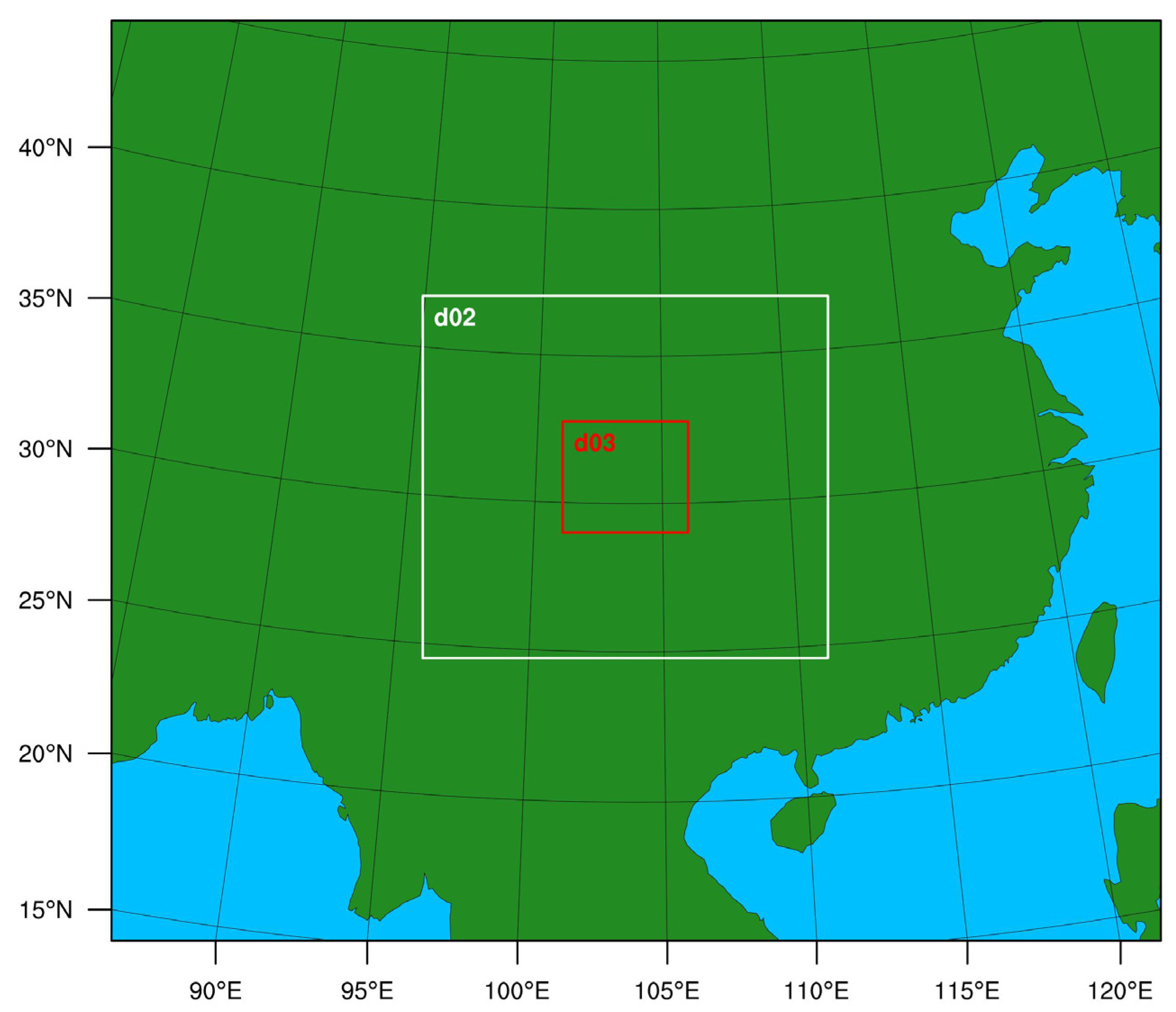
All experiments in this meteorological model numerical simulation used WRF version 3.9, and a Lambert projection was used in the model. During the WPS preprocessing, the latitude of the center point of the simulation area was set to 30.778° N, and the longitude was set to 103.969° E. The ratio of the distance between the innermost layer and the outer layer of the domain mesh was usually set to 1:3. We set the grid spacing of domain 1 to 27 km, and the horizontal grid in the simulation range constituted a grid network of 146 × 128. We set the grid spacing of domain 2 to 9 km, and the horizontal grid in the simulation range constituted a grid network of 169 × 151. We set the grid spacing of domain 3 to 3 km, and the horizontal grid in the simulation range constituted a grid network of 157 × 139. The nested regions in the WRF simulation settings are shown in
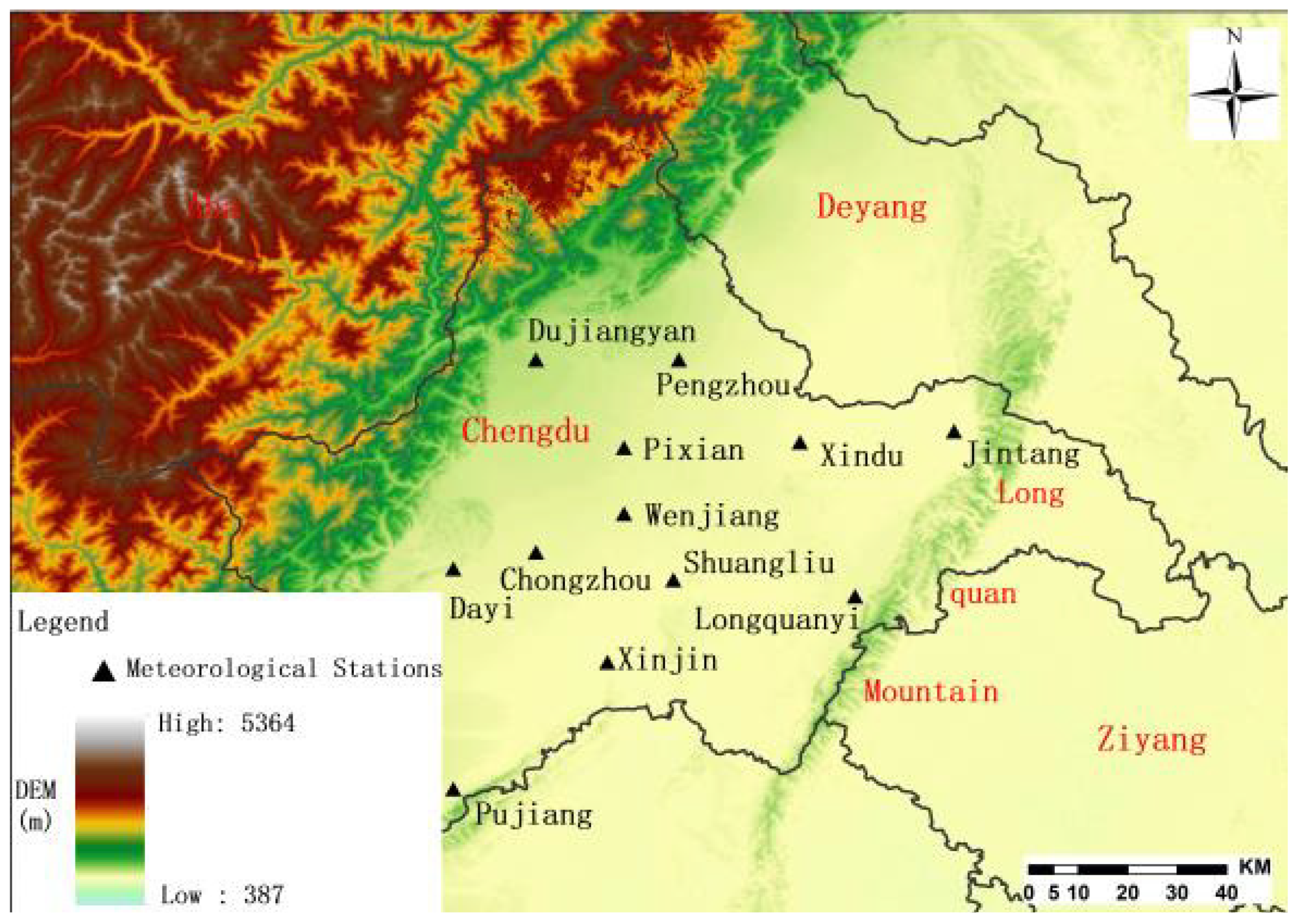
Figure 1. To ensure the accuracy of the experimental results, this paper uses the domain 3 simulation results for analysis, and the wind speed and temperature in the WRF simulation results are verified using hourly data from weather stations in the study area. The location of the weather station in Chengdu is shown in
Figure 2. During the comparison and verification of the simulation results, the NCL (The NCAR Command Language) postprocessing language was used to program the data at the corresponding latitude and longitude points. Then, rcm2points (function in the NCL) is used to interpolate the data on the curve grid to the latitude and longitude of the weather station, which is required to verify the results, and the simulation results are evaluated relative to the corresponding meteorological site data. The meteorological stations in the study area are assessed using an average spatial method. This section focuses on the evaluation of temperature and wind speed simulation effects.
For comparison, reference is made to the baseline wind speed and temperature values obtained by Emery et al. [
18]. To evaluate the simulation capabilities of the WRF model, the indicators listed in
Table 1 and
Table 2 are used to select the parameterization scheme that best matches the actual temperature and wind speed.
In terms of the microphysics parameterization scheme, Lin and WSM3 (WRF Single–Moment 3 class) were selected; SLAB, Noah, and RUC (Rapid Update Cycle) were selected for the land surface models; Dudhia and CAM(Convection-allowing Model) were selected for the shortwave radiation, and RRTM(Rapid radiative Transfer Model) and CAM were selected for the longwave radiation. The above parameters were combined into 12 groups of schemes, and the results were simulated separately and compared with the measured data. Finally, the parameterization scheme suitable for the study area was obtained. The 12 sets of parameterization schemes are given in
Table 3. Moreover, the other physical parameterization schemes selected in this paper are given in
Table 4, and the cumulus convection scheme was used for domain 1 and domain 2.
2.3.3. WRF Model Land-Use Data Assimilation
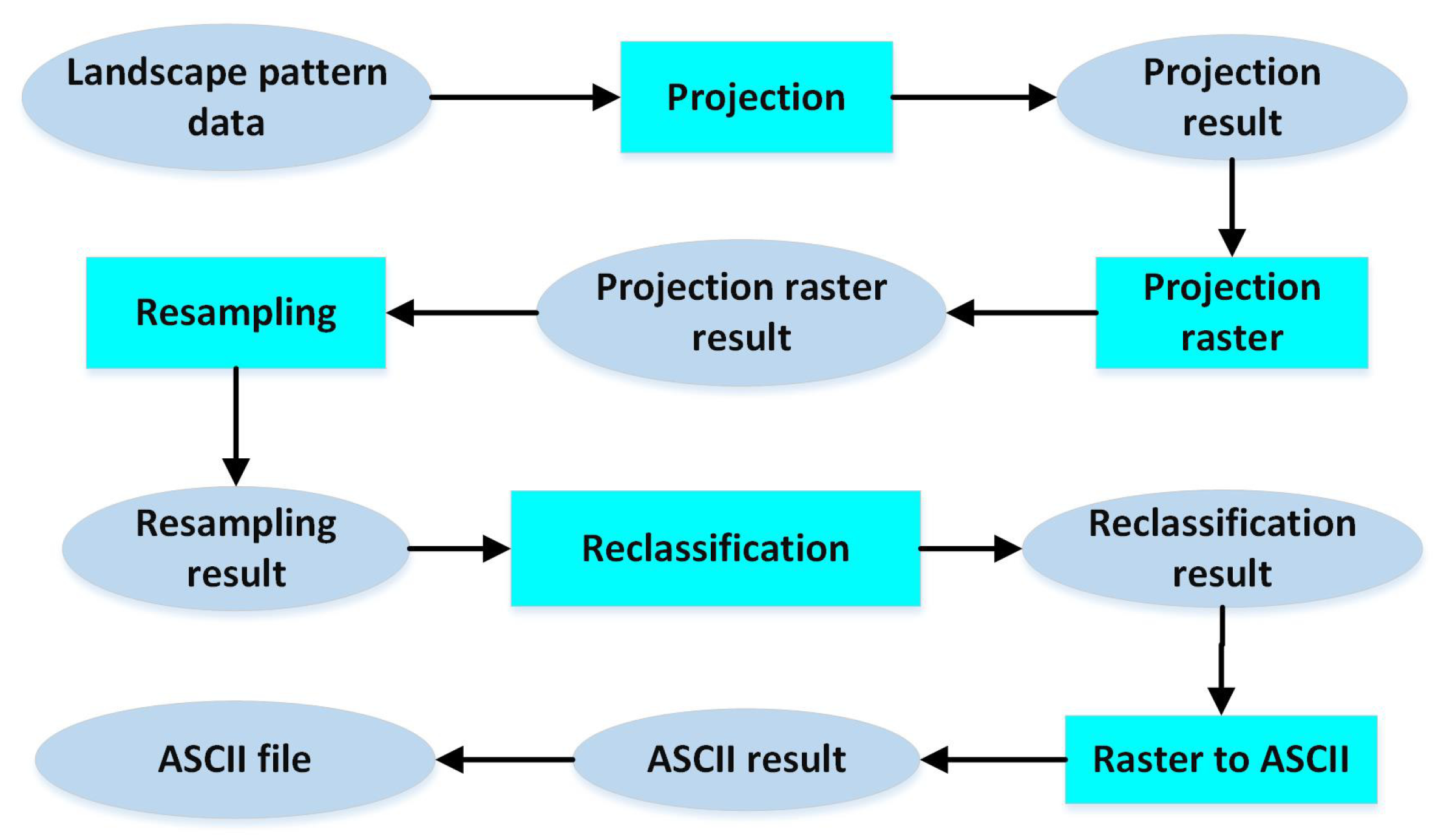
Using ArcGIS (Geographic Information System Software), the 1980 and 2015 land-use data were reprojected into WRF-identifiable WGS84 (World Geodetic System 1984) ellipsoids. The data were reclassified according to the USGS24 (United States Geological Survey 24 categories) code, and then the land-use data were converted to ASCII (American Standard Code for Information Interchange) format in the GEOG (Geography) (Terrain processing under WPS) form defined during WPS (The WRF Preprocessing System) preprocessing. Then, in the WRF model WPS preprocessing module, the FORTRAN (Formula Translation) program was placed in the GEO (Geography) folder, and the ASCII format file processed by ArcGIS was called. The ASCII files were formatted using the official C-language programming script provided in the WRF model terrain folder. Finally, the original land-use_30s files were replaced, the index file was defined, the land-use_30s_1980 and land-use_30s_2015 files were created, and the namelist file was modified. The WRF model land-use data assimilation process is shown in
Figure 3.
2.3.4. Numerical Simulation of Air Quality
The operation of the WRF-Chem air quality model first uses the meteorological module in the WRF model, followed by the chemical module in the Chem model [
19,
20,
21]. The Weather Research Forecasting Model with the Chemistry model is an online coupling of physical meteorological processes in the WRF model with chemical processes in the Chem model. The WRF-Chem air quality simulation model is roughly the same as the mesoscale WRF meteorological numerical simulation model. The only difference is that the namelist file in the WRF-Chem model has more parameters and settings for the chemical module than does that of the WRF model.
This study used the WRF model data assimilation method in
Section 2.3.3 to convert high-precision land-use data from Chengdu in 1980 and 2015 to mesoscale WRF meteorological models that could be used as input data, and these data were combined with the parameterization scheme and the chemical part of the Chem model.
Taking the heavily polluted days in December 2015 as an example, after the numerical simulations responded to changes in the land-use data for urban development, the effect of the model on the simulation results of PM
2.5 was studied. The simulation results were verified using the hourly concentration of PM
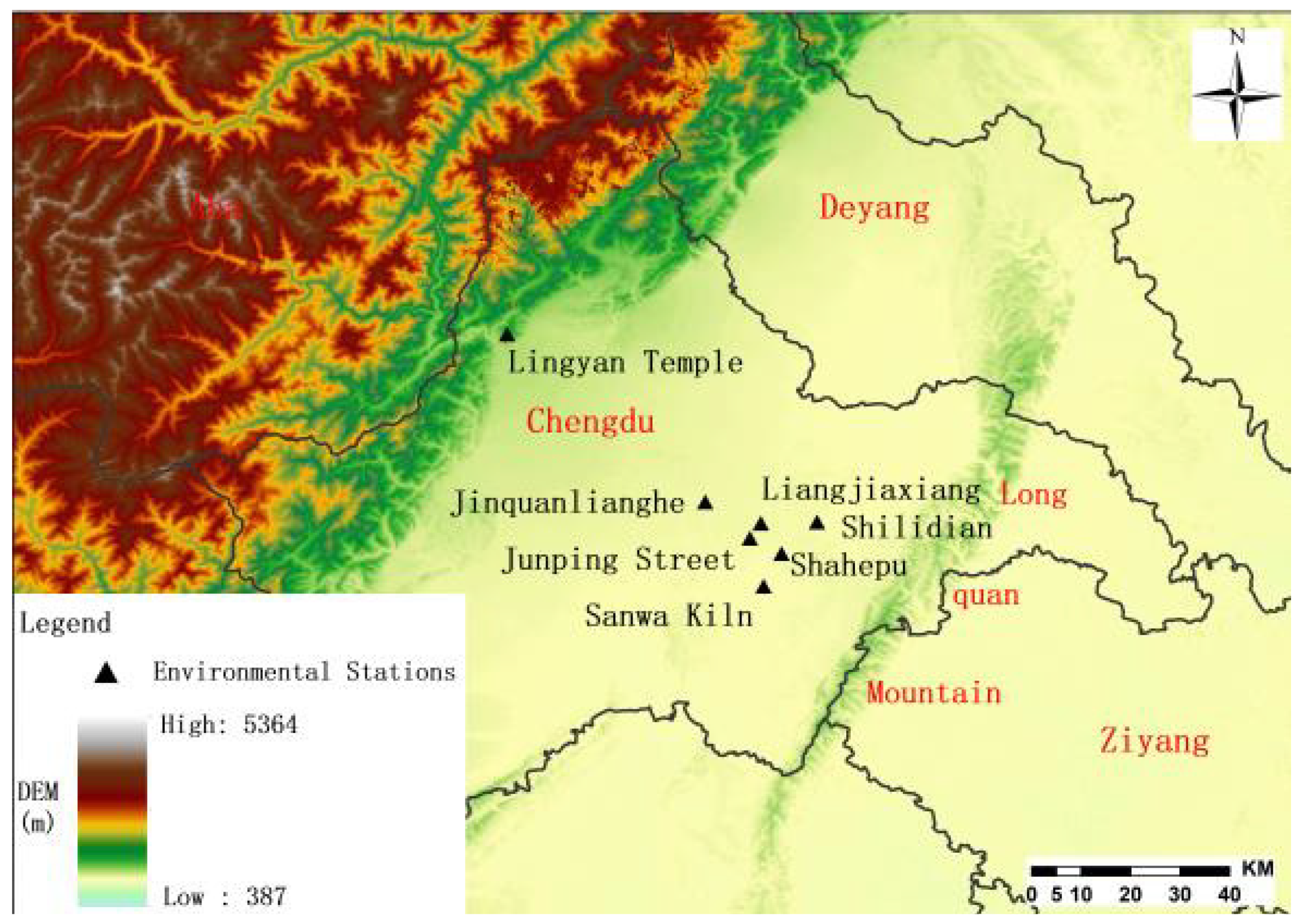
2.5 from the Chengdu Environmental Monitoring Station from 26 December 2015, to 31 December 2015. The location of the environmental monitoring station in Chengdu is shown in
Figure 4.
During the comparison and verification of the simulation results, the hourly concentration in Chengdu simulated by WRF-Chem was compared with the hourly monitored concentration from Chengdu. In the comparison and verification of the simulation results, the NCL (The NCAR Command Language) postprocessing language was used to program the data at the corresponding latitude and longitude points, the rcm2points function in the NCL language was used to interpolate the data on the curve grid to the latitude and longitude of the environmental monitoring station required for the verification of the results, and the simulation results were then evaluated relative to the corresponding environmental monitoring station data. The Environmental stations in the study area are assessed using an average spatial method. This section focuses on the evaluation of PM2.5 simulation effects.
This paper mainly evaluates the effects of simulating the concentration of a basic atmospheric pollutant, PM
2.5. In comparison, the method used by Liang Jin et al. [
22] was used to evaluate the original underlying surface data and the model simulation ability after replacing the underlying surface data.
In this paper, the correlation coefficient (R), standard deviation (Bias), and limit error are used to evaluate the simulated PM
2.5 concentration. To evaluate the simulation capabilities of the WRF-Chem model, the indicators listed in
Table 5 were used to select the parameterization scheme that best matched the actual PM
2.5 concentration. The limit error is the percentage of the total number of samples that meet the requirement of 0.5 ≤ analog value/observation value ≤ 2, and the closer this value is to 100%, the better the simulation results.
2.3.5. Statistical Methods
This study uses statistical methods. The method was mainly applied in two parts. The first part was used to analyze and evaluate the wind speed, and temperature data monitored by meteorological stations and compare these values with the values simulated by the WRF model, and the second part was used to analyze and evaluate the results of pollutant concentrations at the environmental monitoring sites and compare these values with those simulated by the WRF-Chem air quality model.
3. Results and Discussion
3.1. Study on the Characteristics of Urban Land-Use Changes in Response to Urban Development
3.1.1. Basic Situation of Land-Use/Cover in Chengdu
As shown in
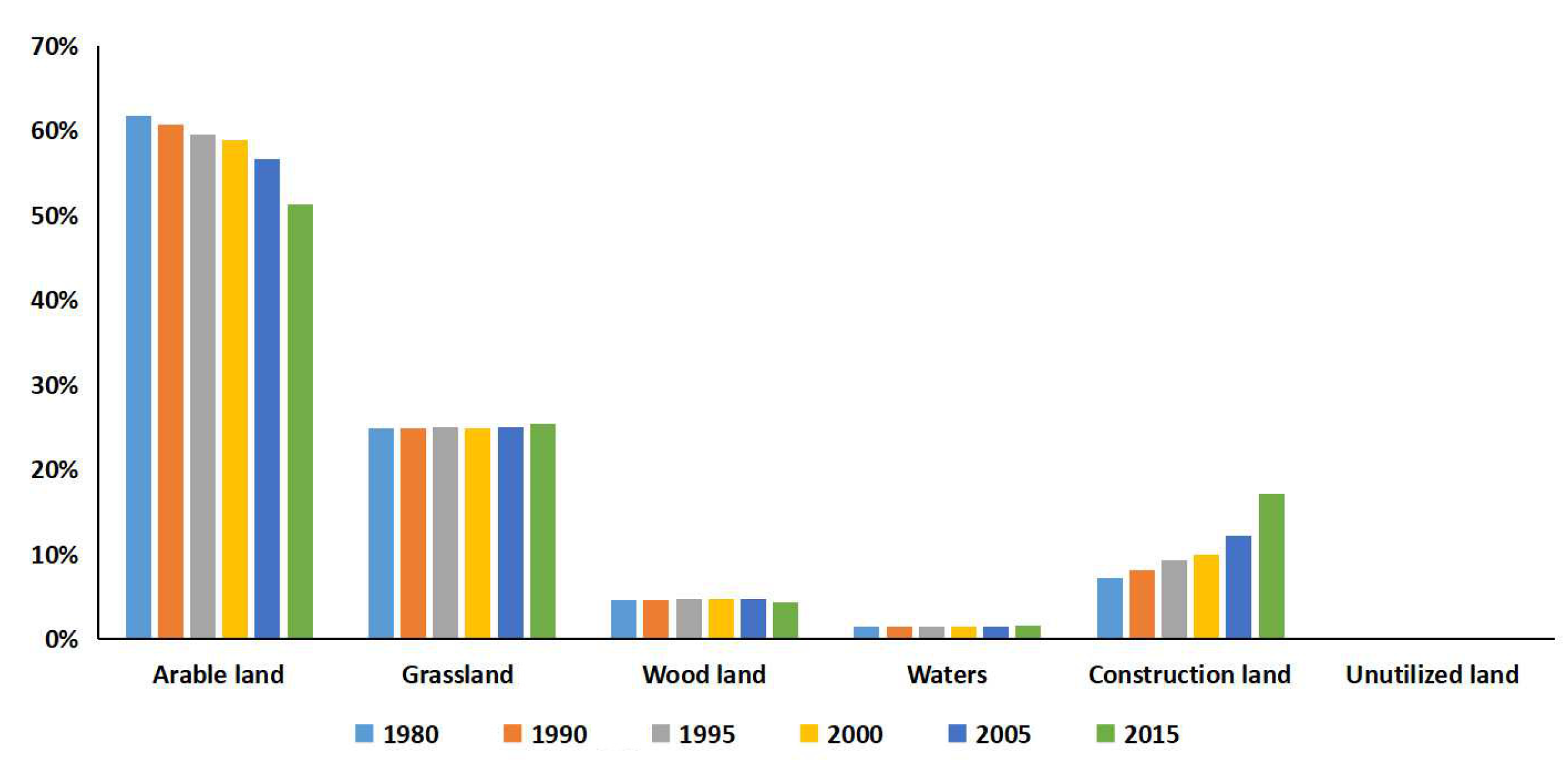
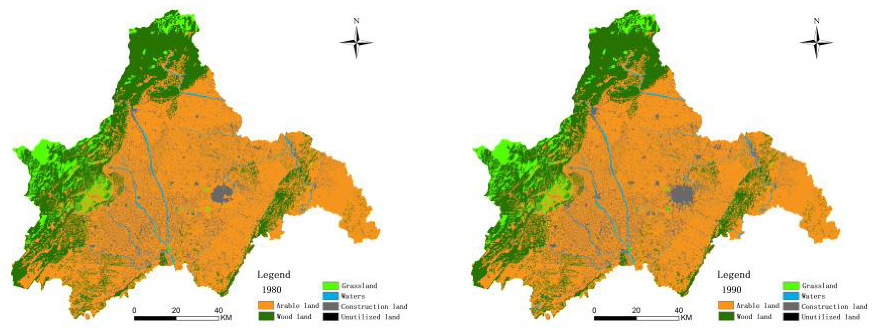
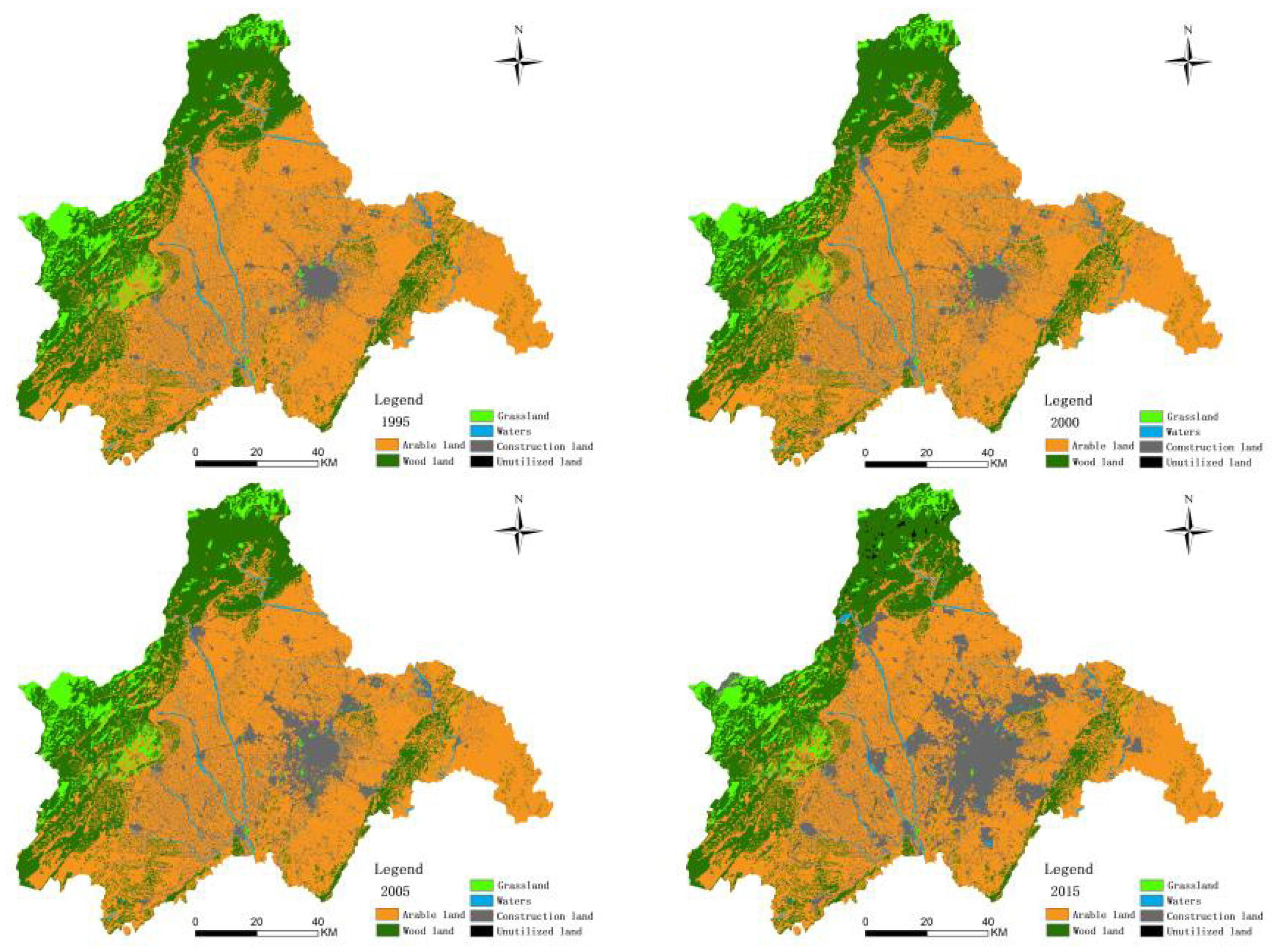
Figure 5 and
Figure 6, during the study period, the cultivated land area accounted for 61.67% of the total land area in 1980, followed by grassland, which accounted for 24.88% of the total land area. Forestland area accounted for 4.67% of the total land area. The water area and unused land area accounted for small proportions of the total land area compared with the cultivated land type, and the difference ranged from 50 to 60%. Cultivated land and construction land were the land-use types that exhibited the most obvious changes in Chengdu from 1980 to 2015. The proportion of the total area of cultivated land from 1980 to 2015 continuously decreased. Compared to the 1980’s, cultivated land decreased by 10.45%, and the forestland decreased by 0.284% in 2015. At the same time, the area of construction land increased by 9.924%, and the grassland area increased by 0.484%. These results show that the urban development in Chengdu is rapid and that during the process of urban development, urban green construction, the improvement of people’s living comfort, and efforts toward a green development path should be the focus in Chengdu.
Taking construction land as the main indicator of urban expansion, construction land was extracted as a representative of the construction area, and ArcGIS (Geographic Information System Software) was used to extract construction land in 1980, 1990, 1995, 2000, 2005, and 2015 to reflect the construction area. In 1980, the construction area of Chengdu accounted for 7.299% of the total area of Chengdu. In 1990, the construction area accounted for 8.195% of Chengdu’s total area. In 1995, the construction area accounted for 9.356% of Chengdu’s total area. In 2000, the construction area occupied 10.048% of Chengdu. In 2005, construction area accounted for 12.238% of Chengdu’s total area. In 2015, construction areas accounted for 17.223% of Chengdu’s total area. As shown in
Table 6, it is obvious that the proportion of construction area in Chengdu continued to increase from 1980 to 2015, and the urban expansion was very significant.
3.1.2. Dynamic Changes in Landscape Patterns
The landscape pattern index was analyzed at the landscape scale, as shown in
Table 7. The changes in patch number and patch density in the study area varied over the 35-year period, and the specific changes were manifested as decrease-increase-decrease. The LPI (Largest patch index) and CONTAG (Contiguity) index showed decreasing trends over the 35 years, which indicates that the degree of landscape fragmentation gradually increased. Between 2000 and 2005, the LPI fell sharply from 29.4787 to 13.2676, and the sharp drop may have been due to the “10
th Five-Year Plan for China’s National Economic and Social Development” from 2000 to 2005. Chengdu responded to the call for vigorous development; thus, the speed of urban expansion surged. The area under construction in the city area expanded from 348.25 km
2 in 2000 to 558.73 km
2 in 2005, and the urbanization rate increased from 34.13% in 2000 to 50.3% in 2015. In 1980, the IJI value was 48.9112, and this value increased to 51.9101 in 2015, indicating an increase in proximity. The DIVISION (Landscape Division) index increased from 0.8638 in 1980 to 0.9476 in 2015, indicating an increase in landscape separation. The SHDI (Shannon’s diversity index) and SHEI (Shannon’s evenness index) continued to increase between 1980 and 2015, showing that with the changes in land-use and the influence of human activities over the past 35 years, the landscape richness and evenness of Chengdu increased.
3.2. Study on the Influence of Urban Land-Use Changes on Meteorological Factors
This section converts the land-use data from 1980 into a WRF model and simulates the wind speed and temperature during the atmospheric-pollution period in Chengdu from 26 December 2015 to 31 December 2015. To comprehensively consider the initial field and boundary conditions, during the WRF simulation, the initial simulation time was set to 22 December 2015, and the simulation start time was four days earlier than the research time.
3.2.1. Simulating the Changes in Meteorological Factors Using WRF Numerical Data from 1980 Urban Land-use Data
3.2.1.1. Analysis of Wind Speed Results Using 1980 Land-Use Data
Meteorological elements in the wind field are closely related to the formation and evolution of atmospheric pollutants. On the one hand, the wind transmits pollutants in the direction of its movement, and on the other hand, the wind plays a role in the diffusion and dilution of pollutants during the occurrence of pollution. Some recent scholars have found that the simulation results will be slightly higher when the actual wind speed is low, possibly because the terrain of the underlying surface of the study area is complex, and the parameterization scheme is biased. In
Table 8, the four groups of data that meet the statistical reference values of
Table 8 are selected. The average deviation (MB) is less than 0.5 m/s, the coincidence index (d) is greater than 0.6, the root means square error (
) is less than 2 m/s, and the correlation coefficient was tested at the 99% confidence level. The optimal value of the coincidence index (d) is up to 0.688 (group 4), that of the hit rate (HR) is up to 0.607 (group 10), that of the correlation coefficient (R) is up to 0.467 (group 4), and that of the average deviation (ME) is at least 0.004 m/s (group 3). The minimum root means square error is 0.597 m/s (group 3), and the minimum mean error is 0.458 m/s (group 4). Through the above analysis, the matching index (d) and the correlation coefficient (R) of group 4 were found to be the highest of the four combinations, and the average deviation, average error, and root means square error were also lower in the four combinations, indicating that when simulating urban wind speed changes, the WSM3 microphysical scheme, and the SLAB land surface scheme in group 4 are the most suitable.
3.2.1.2. Analysis of Temperature Results Using 1980 Land-use Data
Table 9 shows three sets of data that meet the statistical reference values. The correlation coefficient between the simulation results and the site comparison was greater than 0.8, and the correlation coefficient was significant at the 99% confidence interval. In terms of the optimal values, the coincidence index reached 0.941 (group 4), the hit rate reached 0.639 (group 4), the correlation coefficient reached 0.882 (group 4), the mean deviation reached a minimum of 0.118 °C (group 4), the root mean square error reached a minimum of 1.316 °C (group 4), and the mean error reached a minimum of 0.974 °C (group 4). Through the above analysis of the statistical results of the temperature formula, the group 4 coincidence index and the correlation coefficient were found to be the highest among the four combinations. The mean deviation, mean error, and root mean square error was also the lowest in group 4 among the four combinations. Compared with the other combinations, the mean deviation, mean error, and root mean square error of group 4 were the lowest. When simulating the trend of temperature changes in Chengdu, the results simulated by the parameterization scheme in group 4 are close to the actual situation.
3.2.2. Simulating Changes in Meteorological Factors Using WRF Numerical Data from 2015 Urban Land-Use Data
3.2.2.1. Analysis of Wind Speed Results Using 2015 Land-use Data
As shown in
Table 10, the wind speed was simulated after the 2015 land-use data were placed into the model, and the wind speed simulation results from the 1980 land-use data (hereinafter referred to as the original data) were compared with the observations at the meteorological sites. Compared with the original data, the correlation coefficient increased by 0.045, the coincidence index increased by 0.025, and the hit rate increased by 0.016 in 2015. The average deviation decreased by 0.04 m/s, the average error decreased by 0.059 m/s, and the root means square error decreased by 0.055 m/s. Upon using the 2015 land-use data, the wind speed simulation correlation coefficient reached 0.512, showing a medium linear correlation characteristic, and the coincidence index reached 0.713. Upon using the land-use data from 2015, compared with the original data in
Section 3.2.1.1, the coincidence index and the correlation coefficient improved, and the simulation results were close to the true values.
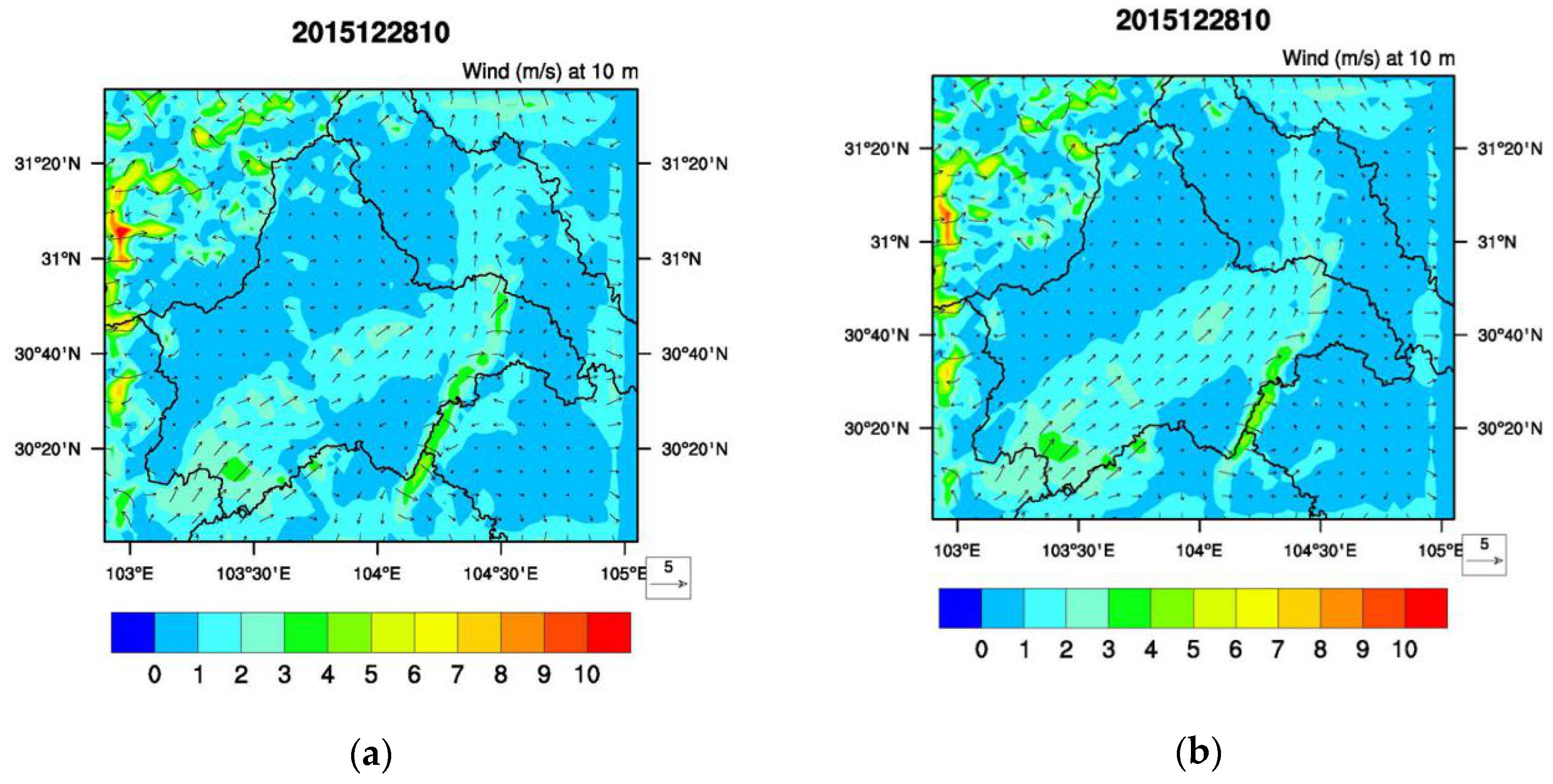
Figure 7 shows the averages of the WRF wind speed results over the entire area of Chengdu using the 1980 and 2015 land-use data. The land-use data from the two periods were basically the same in the wind speed simulations, and the maximum and minimum changes in the wind speeds could be simulated. However, the comparison found that the simulation results obtained using the 1980 land-use data were slightly higher than the simulation results obtained using the 2015 land-use data, and the 10-m average wind speed decreased by 0.36 m/s after the overall land-use changed in the study area. The results in
Section 3.1 indicate that the average wind speed decreased because the proportion of construction land in Chengdu relative to the total area of Chengdu increased from 7.299% in 1980 to 17.223% in 2015. The urban construction area was enlarged, and the urban buildings became densely distributed, which hindered the wind field and caused the wind direction to change. Under the trend of increasing surface roughness, friction, and dragging force, the ground wind field changed, and the advection and convection abilities of the flow field in the urban area weakened, resulting in a decrease in the wind speed in the near-surface layer.
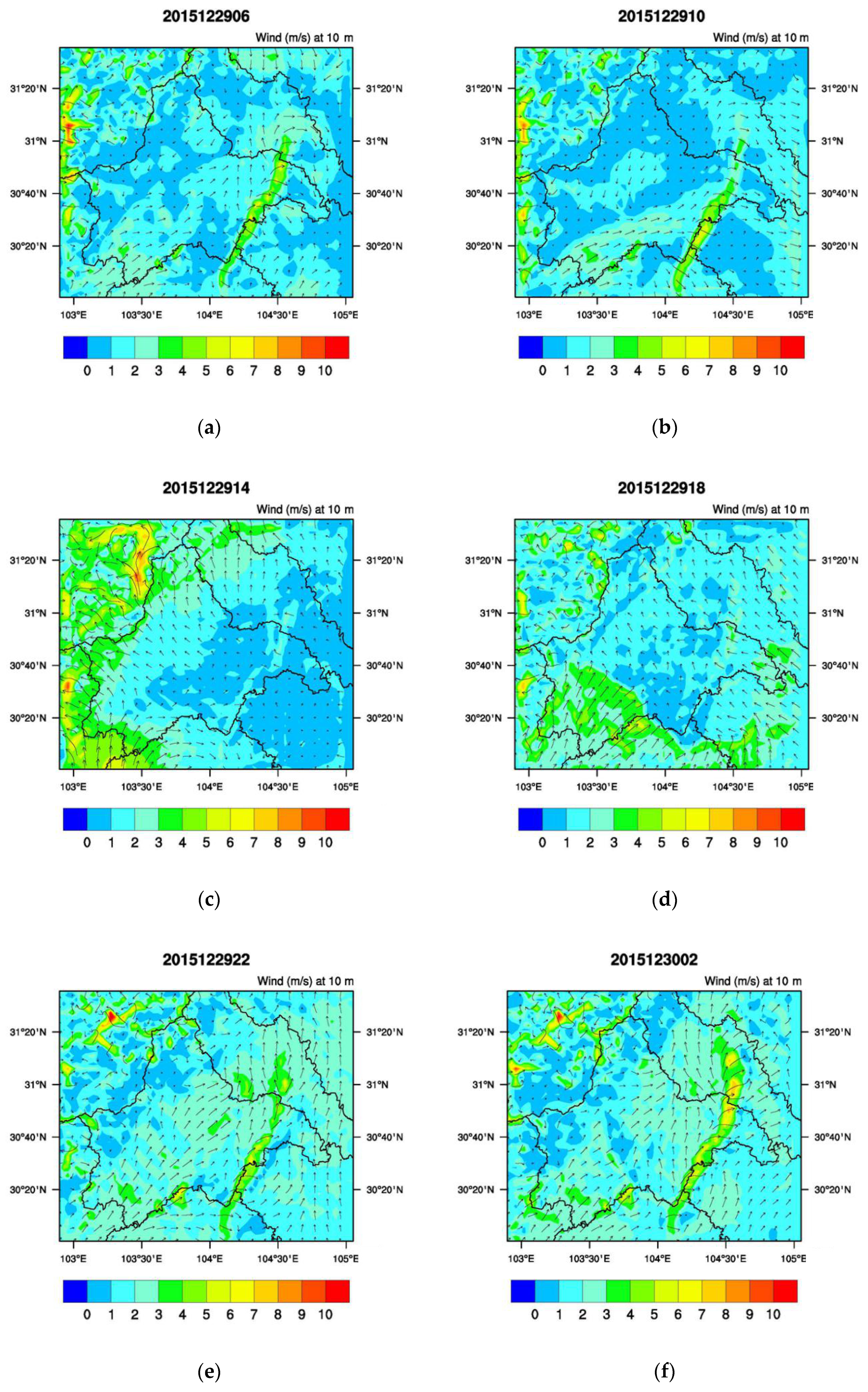
Figure 8 shows the wind speed results for Chengdu produced by the WRF model using the group 4 parameterization scheme and the 2015 land-use data during the atmospheric-pollution period on 29 December 2015. At 06 o’clock, the wind speed in the area of Longquan Mountain in Chengdu was 4–6 m/s, the wind speed in the upper part of Longquan Mountain was 2–3 m/s, the wind speed in the lower part was slightly lower at 0–2 m/s, the wind blew from the lower left side of Chengdu, and the mountain stream flowed through Longquan Mountain. The wind crossed the mountain, flowed to the leeward slope, and entered the right side of Longquan Mountain. At 10 o’clock, the wind speed on the left side of Chengdu was mostly 0–1 m/s and was 1–2 m/s over a small part on the right side of the city, while the wind continued to flow to the right side of Longquan Mountain. At 14 o’clock, the wind speed over Longquan Mountain decreased to 1–2 m/s, and the wind speed on the left and right sides of Longquan Mountain decreased to 0–1 m/s. At 18 o’clock, the wind speed at the lower left side of Chengdu increased, and the proportion of wind speeds at 1–2 m/s in the city increased. At 22 o’clock and 2 o’clock the next day, the wind speed in Chengdu gradually increased to 2–3 m/s. The simulation results indicate that the group 4 parameterization scheme can simulate the influence of the Chengdu terrain on the wind speed. The slow airflow on the left side of Longquan Mountain brings the airflow into the right area along the bottom of the mountain. The air moving at higher speeds meets Longquan Mountain, which changes the direction of motion. Then, as Longquan Mountain facilitates climbing, the air rises over Longquan Mountain, forms an updraft, and moves over the top of Longquan Mountain, bringing the airflow to the right side of the mountain. Longquan Mountain has a significant impact on the near-surface flow field around Chengdu.
3.2.2.2. Analysis of Temperature Results Using 2015 Land-Use Data
The temperature simulation results after the land-use data from 2015 were placed into the model are shown in
Table 11, and the temperature simulation results when the 1980 land-use data (hereinafter referred to as the original data) were used were compared with the observations at the meteorological sites. The simulation results in 2015 changed according to various indicators. Compared with the original data, the correlation coefficient increased by 0.021, the coincidence index increased by 0.006, and the hit rate increased by 0.066. After using the 2015 land-use data, the temperature simulation correlation coefficient reached 0.903, and the coincidence index reached 0.947. When the simulation results of the 2015 data were compared with the original data in
Section 3.2.1, it was found that the data in 2015 were improved in terms of the coincidence index and correlation coefficient, and the simulation results were close to the true values.
Figure 9 shows the average WRF temperature results across Chengdu obtained using the land-use data from 1980 and 2015. The temperature simulations using the two sets of data resulted in basically the same trends, and both data sets could simulate the maximum and minimum values of the temperature changes. However, the comparison revealed that the temperature simulation results obtained using the 1980 land-use data were slightly lower than the simulation results obtained using the 2015 land-use data. The average temperature at 2 m increased by 1.1 °C after the change in the overall land-use in the study area. The results of
Section 3.1 indicate that the average wind speed decreased because the proportion of construction land in Chengdu relative to the total area of Chengdu increased from 7.299% in 1980 to 17.223% in 2015. The heat storage and heat dissipation capacity also changed, and the ground radiation became the main direct heat source for the temperature rise.
Figure 9 shows that due to the changes in the urban land-use type, the process of urbanization development has continuously catalyzed the intensity of social and economic activities, promoted urban energy consumption, and artificially released heat. Moreover, the wind speed in the city has become slow, ventilation has been blocked, and heat cannot be easily dissipated. These conditions caused the temperature of the city to become higher than that of the suburbs and exacerbated the urban heat island phenomenon. In the WRF temperature map simulated using the 2015 land-use data, the high-temperature area was larger than that in the 1980 simulation results. In the results simulated using the 1980 land-use data, the temperature range of Chengdu was mostly 8–14 °C. However, the results simulated using the 2015 land-use data indicate that the temperature range was mostly 9–16 °C.
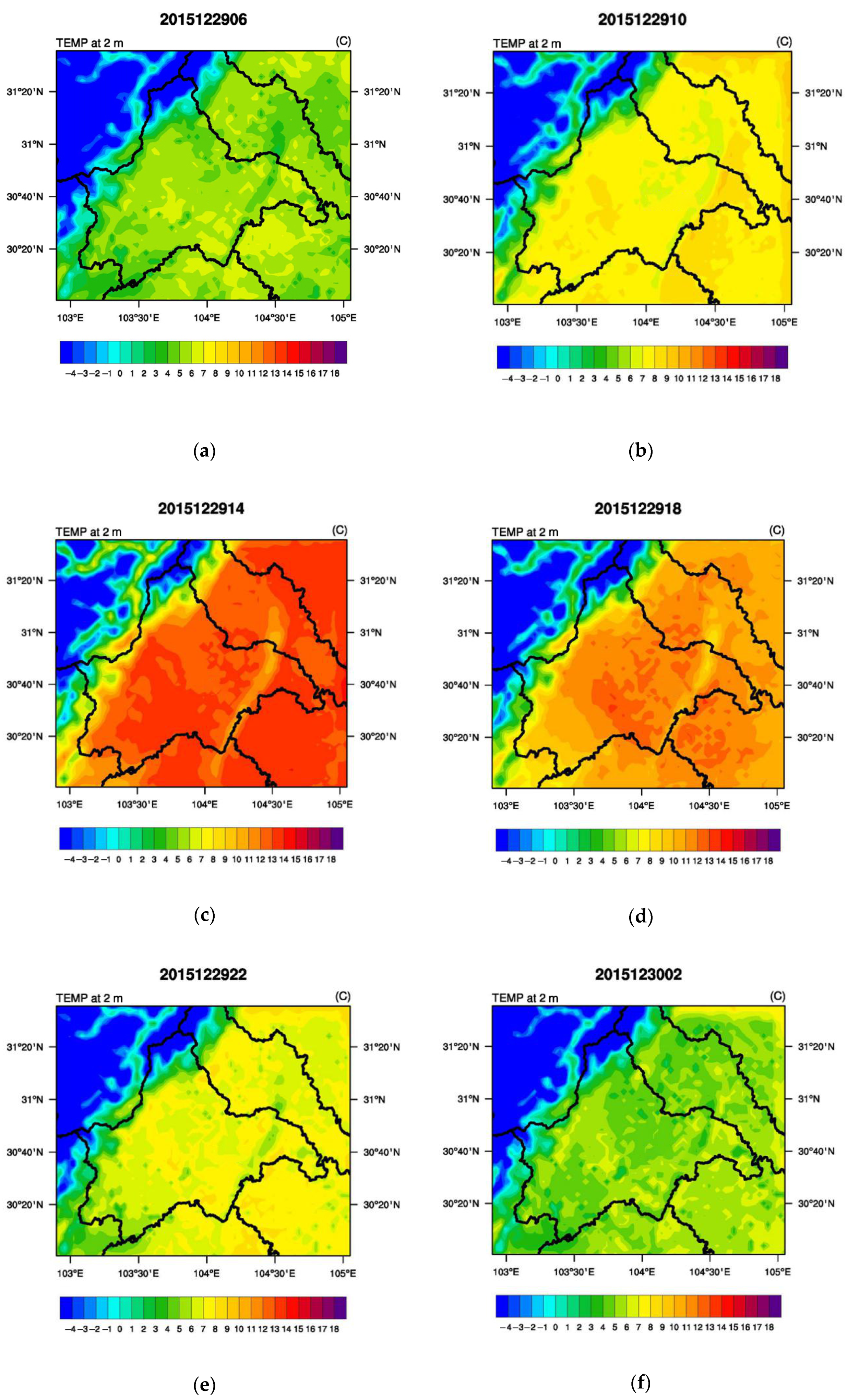
Figure 10 shows the WRF temperature simulation results obtained using the 2015 land-use data and the group 4 parameterization scheme during an atmospheric pollution event in Chengdu on December 29, 2015. Chengdu is located in the Sichuan Basin, where the wind speed is low, and the airflow is weak. Due to extensive radiation, the temperature is high during the day, and the temperature drops significantly at night due to decreased radiation, resulting in prominent temperature differences in the interior of the basin. At 06 o’clock, the temperature in Chengdu was 4–7 °C and the temperature at Longquan Mountain was 2–4 °C. At 10 o’clock, the temperature in most parts of Chengdu was at 7–8 °C. At this time, the temperature in the area of Longquan Mountain was still 2–3 °C lower than that in Chengdu. In the afternoon, the amount of heat stored on the ground continued to increase, the longwave radiation released from the outside continued to increase, and the temperature continued to rise. At 14 o’clock, a large area of Chengdu reached the highest temperature of 12–15 °C. At 18 o’clock, the temperature gradually decreased, and the change continued until 22 o’clock. The temperature in Chengdu was 6–8 °C. In the early morning of the next day, the temperature in Chengdu again ranged from 4–6 °C. Longquan Mountain is approximately 1000 m above sea level; hence, less heat is generated after longwave radiation is released from the ground due to the long distance from the ground. Therefore, the temperature on Longquan Mountain is slightly lower than the surrounding temperature most of the time. The simulation results indicate that the group 4 parameterization scheme can simulate the influence of the terrain on the temperature very well.
3.3. Impact of Urban Land-use Change on Air Pollution Simulation by WRF-Chem
This section analyzes and studies the air pollution process in Chengdu from 26 December 2015 to 31 December 2015. The changes in the PM2.5 concentration before and after the land-use data (1980 and 2015) were changed were explored. To comprehensively consider the initial field and boundary conditions of the aerosol, when WRF-Chem was implemented, the initial simulation time was set to 22 December 2015 and the simulation start time was four days earlier than the research time.
In the parameterization scheme, the WRF model parameterization scheme identified in
Section 3.2 was used as the input for the WRF model parameterization scheme (Group 4). The WSM3 option was selected for the microphysical scheme in the WRF part, the CAM option was selected for the shortwave radiation scheme, the SLAB option was selected for the land surface scheme, and the CAM option was selected for the model input in the longwave radiation scheme. The chemical module combining GOCART (Simple and efficient aerosol solution) and RADM2 (Regional Acid Deposition Mechnism) was selected for the Chem part, and the MEIC emission source data from
Section 2.2.5 were brought into the WRF-Chem model for simulation. The physical and chemical parameter schemes are shown in
Table 12.
Analysis of PM2.5 Concentration Results Using the WRF-Chem Model
As shown in
Table 13, the PM
2.5 concentration simulation results after the 2015 land-use data were included in the model, and the results obtained when the 1980 land-use data were used in the model (hereafter referred to as the original data) were compared with the observations from the meteorological sites.
The correlation coefficient of the 1980 land-use data simulation results with the measured values of the environment was 0.41. After the 2015 simulation results and measured values were evaluated and compared with the original data, it was found that the data simulation results in 2015 increased the correlation coefficient by 0.14, decreased the standard deviation by 0.21, and increased the limit error by 15%.
After using the 2015 land-use data, the correlation coefficient of the PM2.5 simulation results increased to 0.55, and the standard deviation increased from −0.65 in 1980 to −0.44 in 2015. When the simulation results from the 2015 land-use data were compared with the original data, it was found that the land-use data in 2015 improved both the standard deviation and the correlation coefficient, and the simulation results were close to the true values. Although the limit error statistic was less than 50%, the limit error of the pollutant simulation results obtained using the 2015 land-use data was greater than that obtained using the 1980 land-use data. This result shows that the effect of the land-use data in 2015 on the simulation is better than the effect of using the original land-use data. Overall, the 2015 land-use data enabled the WRF-Chem air quality model to simulate pollutant concentrations better.
Figure 11 shows the average PM
2.5 from the WRF-Chem model across Chengdu using the 1980 and 2015 land-use data. When the two land-use data sets were used in the simulation, the trend remained basically the same. Both data sets could simulate the maximum and minimum PM
2.5 changes, but the comparison found that the PM
2.5 simulation results obtained using the 2015 land-use data were slightly higher than the simulation results obtained using the 1980 land-use data. As shown in
Figure 11, the concentration of PM
2.5 in urban areas was higher than that in the suburbs.
Figure 11 shows that the 1980 and 2015 land-use simulation results could accurately reflect the spatial distribution of regional pollutant concentrations. The numerical simulation results show that the values in 2015 were slightly higher than those in 1980, especially in urban areas. The reason for this difference is that the urban area expanded, the underlying surface roughness increased, and the ground friction and dragging effect were both enhanced. The wind speed in the near-surface layer weakened, and the advection and convection capacity of the urban wind field decreased, which caused the migration and diffusion of pollutants in the near-surface layer to decrease, eventually leading to the accumulation of pollutants in urban areas and difficulty in spreading. This condition is also the main reason why urban air quality is not as good as that in nonurban areas.
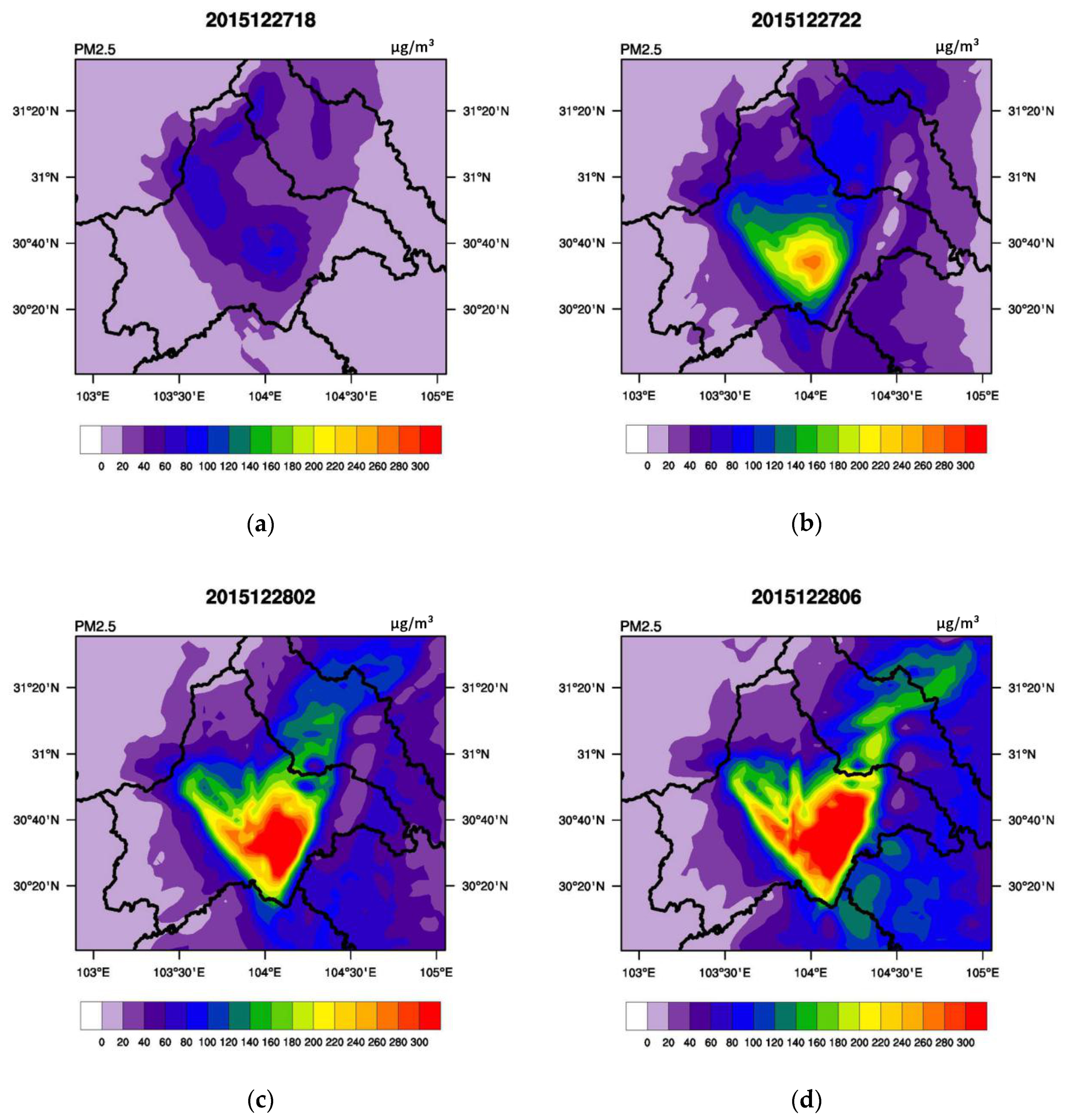
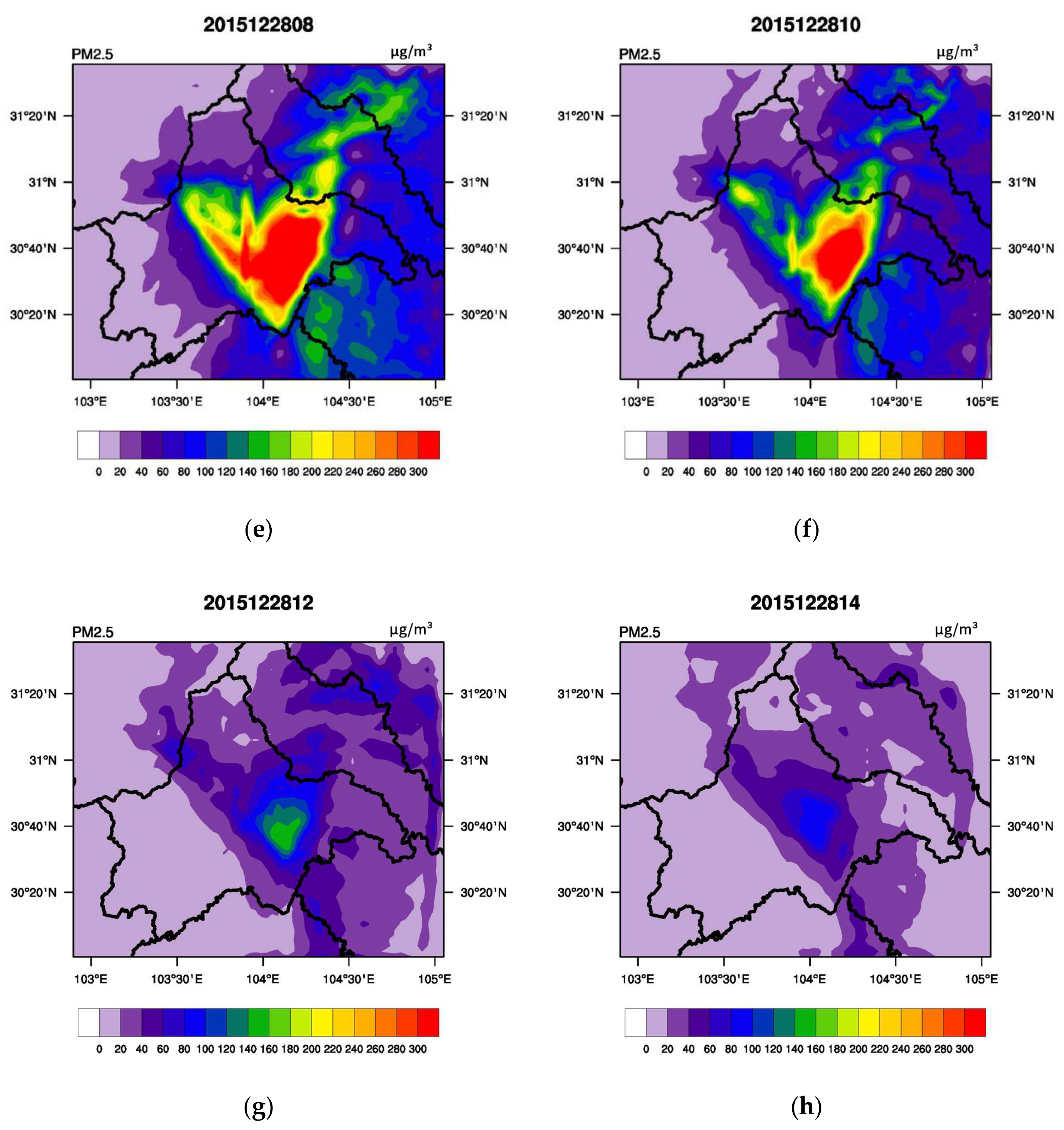
Figure 12 shows the PM
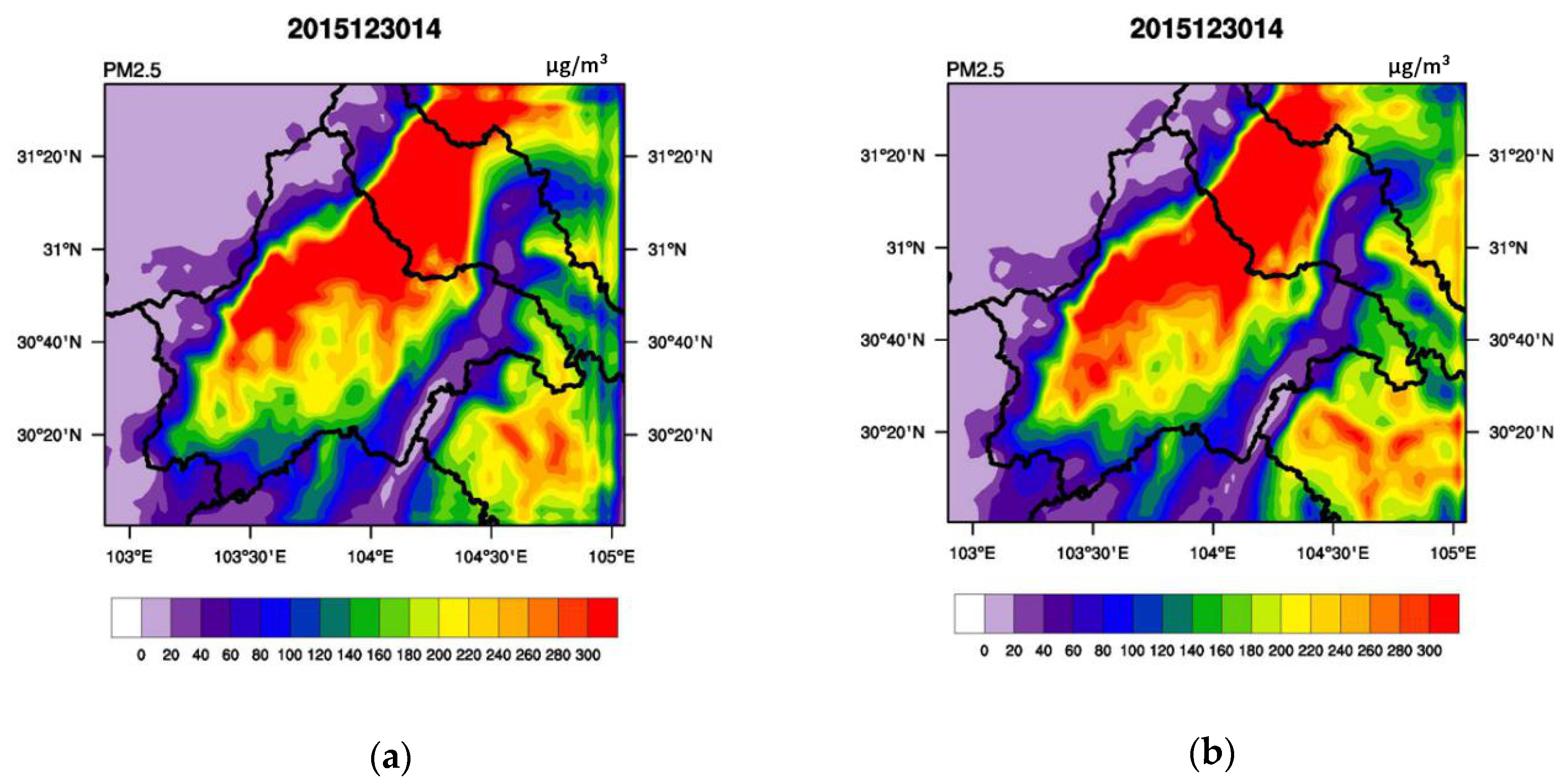
2.5 concentration in Chengdu during the atmospheric pollution period on 27 December 2015, simulated by the WRF-Chem model using the 2015 land-use data. The concentration over a large area in Chengdu was between 20 µg/m³ and 80 µg/m³ at 18:00, and the concentration over a small part was between 80 µg/m³ and 100 µg/m³. The concentration of pollutants began to increase from the second side of Longquan Mountain to the central part of Chengdu, and the concentration of pollutants reached 240 µg/m³ over a small area. The concentration over Longquan Mountain was much lower than that in the urban area. The concentration ranged from 0–40 µg/m³, and the concentration on the right side of Longquan Mountain was 0–60 µg/m³. By the next day at 02:00, the concentration of pollutants continued to increase, and pollutants began to be transmitted to the north-northeast of Chengdu. At the same time, the pollutants spread from the central part of Chengdu to the border area of Chengdu. The highest concentration in the southern part of the Longquan Mountain range reached 80, the concentration in the northern part of the mountain range was 20–60 µg/m³, and the highest concentration reached 100 µg/m³ on the right side of Longquan Mountain. At 06:00 on the next day, the pollutants transmitted to the northeast of Chengdu passed through Deyang City and arrived in Mianyang City. At this time, the pollutants to the left of Longquan Mountain in Chengdu were higher than those in the surrounding areas. At 8:00 on the following day, the pollution in the area on the right side of Longquan Mountain continued to increase, and the pollution concentration over Longquan Mountain was higher than that to the right of the mountain. The pollution area began to decrease at 10:00 on the following day, and the concentrations of pollutants began to decline. The pollutants to the north of Chengdu began to dissipate at 12:00 on the following day, and the concentration decreased. At this time, the concentration of pollutants was high over a small part of Longquan Mountain in Chengdu. In the southwestern part of Chengdu, the concentration was 0–20 µg/m³ at 14:00 on the next day, the concentration of pollutants was mostly 20–80 µg/m³ in the northeast direction, and the concentration reached 100 µg/m
3 over a small part of the study area. The phenomenon in which the pollutant concentration increased in the early morning and evening may be related to human travel. In the morning and evening, automobile exhaust peaks and greatly contributes to traffic pollution. The emissions generated by people’s daily activities make great contributions, and other contributions are made by urban dust.
4. Discussion
From the standard deviation, it can be seen that the simulated pollutant concentrations were lower than the monitored values. The standard deviation of the data in 2015 was −26.4%, and the standard deviation of the data in 1980 was −31.1%. The simulated PM2.5 concentrations were lower than the measured values, which may have occurred because the list of emission sources used by the model is not a detailed list of the true emission sources that localized by the allocation adjustment process after being reported or investigated by various departments. Some “scattering pollution” emissions statistics and yellow-label vehicle emission statistics are not perfect, resulting in an analog value that is lower than the measured value. At the same time, the WRF-Chem simulation results are sensitive to land-use data. When the old land-use data are used, the standard deviation of the evaluation results is too large, and the correlation coefficient is low. The new land-use data were used as replacements in the WRF-Chem model. Compared with the results of the model using the old land-use data (1980), when using the new land-use data (2015), the standard deviation of the simulation results decreased, and the correlation coefficient increased. The reason for this result may be that the land-use data in 2015 are more refined, and the pollution situation in the simulated regional cities is more accurate. According to the time series data, the 2015 data are the same as those in the model simulation year, which is close to the real land-use situation. To ensure the accuracy of the simulation, the land-use data of the current year corresponding to the simulation time should be used in subsequent simulations.
5. Conclusions
1. Between 1980 and 2015, the landscape pattern of the city of Chengdu changed significantly, and the areas of cultivated land and construction land changed the most. The richness and evenness of the landscape structure of Chengdu both increased under the influence of dynamic changes in land-use and human activities on the underlying surface of the city.
2. The wind speed and temperature data revealed that the group 4 parameterization scheme had numerical advantages in terms of the coincidence index and correlation coefficient. Parameterization scheme group 4 was the most suitable for simulating wind speed and temperature changes in Chengdu. The wind speed and temperature simulations that resulted from using the 2015 land-use data and 1980 land-use data were compared. The simulation results were generally better when the 2015 land-use data were used. The coincidence index and correlation coefficient were improved when the 2015 land-use data were used, and the simulation results were close to the true values.
3. The wind speed was greater when the 1980 land-use data were used than when the 2015 land-use data were used. This result occurred because the proportion of construction land increased in Chengdu, and the near-surface layer became rough, while the friction and drag both increased. Acting on the surface wind field, the flow field advection and convection abilities in the urban area weakened, resulting in a decrease in the wind speed in the near-surface layer. This result occurred because the urban construction land-use type gradually replaced other land-use types, resulting in changes in the physical properties of the ground in urban areas, and ground radiation became the main direct source of heat. The increase in the concentration of urban social and economic activities has led to an increase in urban energy consumption and artificially released heat, and the wind speed in the city is slow. The ventilation is blocked, and it is not easy to dissipate heat, which causes the temperature in the city to be higher than that in the suburbs and exacerbates the urban heat island phenomenon.
4. The PM2.5 concentration was simulated using the 2015 land-use data and compared to the measured values. Compared with the original data, both the correlation coefficient and the limit error increased, and the standard deviation decreased when the 2015 land-use data were used, which is consistent with the results of a study by Liangjin. The simulated PM2.5 numerical results indicate that the data from 2015 produced slightly higher results than did the data from 1980, especially in urban areas. The reason for this difference is that the urban area is expanding, the underlying surface roughness is increasing, and the ground friction and dragging effect are being enhanced. The wind speed in the near-surface layer is weakened, and the advection and convection capacity of the urban wind field are declining, which causes the migration and diffusion of pollutants in the near-surface layer to decrease, eventually leading to the accumulation of pollutants in urban areas and difficulty in spreading. This is also the main reason why the air quality in urban areas is not as good as that in nonurban areas.
5. According to the PM2.5 concentration results from the WRF-Chem simulation in Chengdu, heavy pollution occurred in the central part of Chengdu. The concentration of pollutants is high in the central part of Chengdu on the left side of Longquan Mountain, and the concentration on the right side of Longquan Mountain is low. The concentration over Longquan Mountain is much lower than that in Chengdu. Pollution usually spreads on the left side of Longquan Mountain and in the middle of Chengdu, driving the concentration of pollutants in the surrounding areas to consistently increase. Contaminants are usually transported along the Longquan Mountain to the north of Chengdu. The area on the right side of Longquan Mountain is located in the central and western Sichuan Basin, and the four seasons are controlled by the background wind field of the basin. The atmospheric pollutants emitted from Chengdu on the west side of Longquan Mountain are easily transported by the mountain stream with the airflow, which affects the air quality on the east side of Longquan.
6. During the 35 years from 1980 to 2015, urbanization continued to develop. Land-use types such as urban arable land were gradually replaced by buildings and cement pavements, and the roughness increased, resulting in high heat capacity and serious “urban winds” and “urban heat islands”. Over the past 35 years, the population has been increasing in the city, people have become concentrated in the city, and the emissions of smoke have increased. The concentration of industrial combustion has increased. The increase in emissions from transportation has produced more pollutants locally, which has caused the local pollutant amounts to increase. Chengdu is located in the Sichuan Basin, and pollutants are carried outside the basin by either airflow or local pollution due to local emissions. The “urban wind” and “urban heat island” phenomena continue to increase over the course of urban development, which makes the urban wind speed decrease and the temperature increase, causing the urban meteorological conditions to weaken the dilution and diffusion function of pollutants. Pollutants are not easily diffused in the city and instead accumulate; thus, the concentration of pollutants often exceeds the threshold.
Author Contributions
Conceptualization—W.S., Z.L. and X.Lv.; methodology—W.S., Z.L., X.Lv., Y.L. X.Li., H.L. F.M., W.X. and Y.Z.; software—W.S., X.Lv., X.Li., H.L., J.X., F.M., W.X. and Y.L.; validation—W.S., X.Lv., H.L., X.Li. and J.X.; formal analysis—W.S.; data curation, W.S.; writing-original draft preparation—W.S.; writing-review and editing—W.S., Y.Z. and Z.L.; visualization—W.X., Y.Z. and Z.L. All authors have read and agreed to the published version of the manuscript.
Funding
This research was funded by the National Natural Science Foundation of China under grant no. 41771535 and the National Key R&D Program of China under grant no. 2016YFC0208806. The authors thank the reviewers for their numerous valuable comments for improving the manuscript.
Conflicts of Interest
The authors declare that they have no conflict of interest to report.
References
- YU, M.-Y. Dynamic Change Analysis of Urban Green Land in Jinan City Based RS and Geo-information Tupu. Asian Agric. Res. 2011, 1, 94–96. [Google Scholar]
- Biro, K.; Pradhan, B.; Makeschin, F.; Buchroithner, M. Land Use/Land Cover Change Analysis And Its Impact On Soil Properties In The Northern Part Of Gadarif Region, Sudan. Land Degrad. Dev. 2013, 24, 90–102. [Google Scholar] [CrossRef]
- Xu, X.-C.; Cheng, D.-L. Comparative Study on the Human Driving Force of Cultivated Land and Construction Land Use Change in Hubei Province, China. Asian Agric. Res. 2010, 17, 12–16. [Google Scholar]
- Smallidge, P.J.; Leopold, D.J. Vegetation management for the maintenance and conservation of butterfly habitats in temperate human-dominated landscapes. Landsc. Urban Plan. 1997, 38, 259–280. [Google Scholar] [CrossRef]
- Ojala, E.; Louekari, S. The merging of human activity and natural change: Temporal and spatial scales of ecological change in the Kokemäenjoki river delta, SW Finland. Landsc. Urban Plan. 2002, 61, 83–98. [Google Scholar] [CrossRef]
- Guo, E.; Chen, L.-D.; Sun, R.; Wang, Z. Effects of riparian vegetation patterns on the distribution and potential loss of soil nutrients: A case study of the Wenyu River in Beijing. Front. Environ. Sci. Eng. 2014, 9, 279–287. [Google Scholar] [CrossRef]
- Zhao, C.; Tie, X.; Lin, Y. A possible positive feedback of reduction of precipitation and increase in aerosols over eastern central China. Geophys. Res. Lett. 2006, 33, 229–239. [Google Scholar] [CrossRef]
- Wang, W.Y.; Yong, L.I.; Luo, K.L. The geochemical characteristics of selenium and fluorine in soils of Daba Mountains. Geogr. Res. 2003, 22, 177–184. [Google Scholar]
- Li, L.; Lian, S.; Feng, C. Data mining-based detection of rapid growth in length of stay on COPD patients. In Proceedings of the 2017 IEEE 2nd International Conference on Big Data Analysis (ICBDA), Beijing, China, 10–12 March 2017. [Google Scholar]
- Zhou, X.; Chen, H. Impact of urbanization-related land use land cover changes and urban morphology changes on the urban heat island phenomenon. Sci. Total. Environ. 2018, 635, 1467–1476. [Google Scholar] [CrossRef] [PubMed]
- Smink, C.K.; Lassen, C. Environmental Perspectives on Aeromobility and the Development of Experience Spaces. Available online: http://resolver.tudelft.nl/uuid:1f7500a5-c428-4557-9301-9b3a7a5b5d99 (accessed on 29 October 2010).
- Roberts, S. Effects of climate change on the built environment. Energy Policy 2008, 36, 4552–4557. [Google Scholar] [CrossRef]
- Rodríguez, A.; Rodríguez, B. Attraction of petrels to artificial lights in the Canary Islands: Effects of the moon phase and age class. Ibis 2010, 151, 299–310. [Google Scholar] [CrossRef]
- Dong, Y.; Liu, Y.; Chen, J. Will urban expansion lead to an increase in future water pollution loads?--a preliminary investigation of the Haihe River Basin in northeastern China. Environ. Sci. Pollut. Res. 2014, 21, 7024–7034. [Google Scholar] [CrossRef] [PubMed]
- Ji, W.; Han, Y.; Guan, Y. Research on the langdscape spatial pattern of Zhegao watershed based on GIS and RS. Chin. Agric. Sci. Bull. 2017, 1, 5. [Google Scholar]
- Zaripov, R.B.; Martynova, Y.V.; Krupchatnikov, V.N. Atmosphere data assimilation system for the Siberian region with the WRF-ARW model and three-dimensional variational analysis WRF 3D-Var. Russ. Meteorol. Hydrol. 2016, 41, 808–815. [Google Scholar] [CrossRef]
- Brioude, J.; Arnold, D.; Stohl, A. The Lagrangian particle dispersion model FLEXPART-WRF version 3.0. Geosci. Model Dev. 2013, 6, 1889–1904. [Google Scholar] [CrossRef] [Green Version]
- Mandel, J.; Beezley, J.D.; Kochanski, A.K. An Overview of the Coupled Atmosphere-Wildland Fire Model WRF-Fire. Available online: https://arxiv.org/abs/1101.5745 (accessed on 19 November 2019).
- Emery, C.; Tai, E. Enhanced Meteorological Modeling and Performance Evaluation for Two Texas Ozone Episodes; Project Report Prepared for the Texas Natural Resources Conservation Commission; Prepared by ENVIRON; International Corporation: Novato, CA, USA, 2001. [Google Scholar]
- Katinka, P.A.; Kumar, R.; Brasseur, G. Towards a forecasting system of air quality for Asia using the WRF-Chem model. Egu. Gen. Assem. Conf. Abstr. 2013, 15. [Google Scholar]
- Tie, X.; Brasseur, G.; Ying, Z. Impact of model resolution on chemical ozone formation in Mexico City: Application of the WRF-Chem model. Atmos. Chem. Phys. 2010, 10, 8983–8995. [Google Scholar] [CrossRef] [Green Version]
- Liang, J.; Qian, J.; Liu, Z. Simulation of the Influence of Underlying Surface Change on Air Pollutant Concentration in Chengyu Economic Zone (Sichuan). Sichuan Environ. 2013, 32, 49–53. [Google Scholar]
Figure 1.
The nested regions in the WRF simulation settings.
Figure 1.
The nested regions in the WRF simulation settings.
Figure 2.
Map of the meteorological stations in Chengdu.
Figure 2.
Map of the meteorological stations in Chengdu.
Figure 3.
Process used to generate the land-use data.
Figure 3.
Process used to generate the land-use data.
Figure 4.
Map of the environmental monitoring stations in Chengdu.
Figure 4.
Map of the environmental monitoring stations in Chengdu.
Figure 5.
Percentages of land-use types in Chengdu from 1980 to 2015.
Figure 5.
Percentages of land-use types in Chengdu from 1980 to 2015.
Figure 6.
Dynamic changes in land-use in Chengdu from 1980 to 2015.
Figure 6.
Dynamic changes in land-use in Chengdu from 1980 to 2015.
Figure 7.
The 10-m wind speed map simulated using 1980 (a) and 2015 (b) land-use data (local time of 10:00 on December 28, 2015).
Figure 7.
The 10-m wind speed map simulated using 1980 (a) and 2015 (b) land-use data (local time of 10:00 on December 28, 2015).
Figure 8.
The wind speed map using 2015 land-use data (a–f): local time from 06:00 on 29 December 2015 to 02:00 on 30 December 2017.
Figure 8.
The wind speed map using 2015 land-use data (a–f): local time from 06:00 on 29 December 2015 to 02:00 on 30 December 2017.
Figure 9.
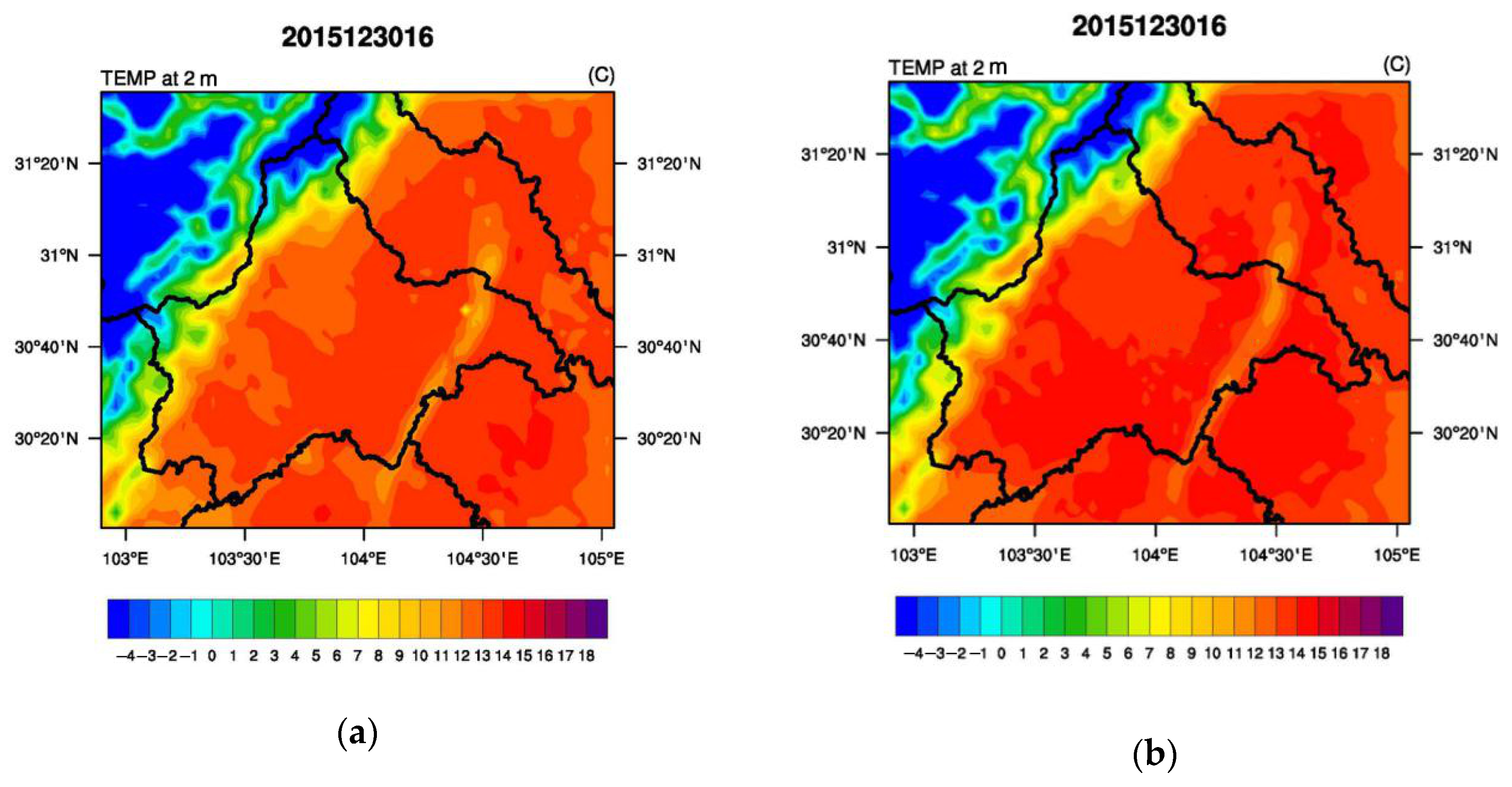
The 2-m temperature map simulated using 1980 (a) and 2015 (b) land-use data (local time at 16:00 on December 30, 2015).
Figure 9.
The 2-m temperature map simulated using 1980 (a) and 2015 (b) land-use data (local time at 16:00 on December 30, 2015).
Figure 10.
The 2-m temperature map obtained using 2015 land-use data, (a–f): local time from 06:00 on 29 December 2015 to 02:00 on 30 December 2015.
Figure 10.
The 2-m temperature map obtained using 2015 land-use data, (a–f): local time from 06:00 on 29 December 2015 to 02:00 on 30 December 2015.
Figure 11.
The PM2.5 concentration map simulated using 1980 (a) and 2015 (b) land-use data (local time at 14:00 on December 30, 2015).
Figure 11.
The PM2.5 concentration map simulated using 1980 (a) and 2015 (b) land-use data (local time at 14:00 on December 30, 2015).
Figure 12.
The simulated PM2.5 concentrations using 2015 land-use data, (a–h): local time from 18:00 on 27 December 2015, to 14:00 on 28 December 2015.
Figure 12.
The simulated PM2.5 concentrations using 2015 land-use data, (a–h): local time from 18:00 on 27 December 2015, to 14:00 on 28 December 2015.
Table 1.
Statistical benchmarks for the wind speed and temperature.
Table 1.
Statistical benchmarks for the wind speed and temperature.
| Category | | | | |
| Temperature | ≥0.8 | ≤±0.5 ℃ | ≤2 ℃ | |
| Wind speed | ≥0.6 | ≤±0.5 m/s | | ≤2 m/s |
Table 2.
Statistical formula.
Table 2.
Statistical formula.
| Statistics | Formula |
|---|
| Correlation coefficient | |
| Conformity index | |
| Average deviation | |
| Average error | |
| Root mean square error | |
| Hit rate | |
Table 3.
The 12 sets of parameterization scheme combinations. (WSM3: WRF Single–Moment 3 class, SLAB: 5-layer diffusion scheme, RUC: Rapid Update Cycle, CAM: Convection-allowing Model, RRTM:Rapid radiative Transfer Model).
Table 3.
The 12 sets of parameterization scheme combinations. (WSM3: WRF Single–Moment 3 class, SLAB: 5-layer diffusion scheme, RUC: Rapid Update Cycle, CAM: Convection-allowing Model, RRTM:Rapid radiative Transfer Model).
| | Parameter Scheme | Microphysics | Land Surface Model | Shortwave Radiation | Longwave Radiation |
|---|
| Group Number | |
|---|
| Group 1 | WSM3 | Noah | Dudhia | RRTM |
| Group 2 | WSM3 | Noah | CAM | CAM |
| Group 3 | WSM3 | SLAB | Dudhia | RRTM |
| Group 4 | WSM3 | SLAB | CAM | CAM |
| Group 5 | WSM3 | RUC | Dudhia | RRTM |
| Group 6 | WSM3 | RUC | CAM | CAM |
| Group 7 | Lin | Noah | Dudhia | RRTM |
| Group 8 | Lin | Noah | CAM | CAM |
| Group 9 | Lin | SLAB | Dudhia | RRTM |
| Group 10 | Lin | SLAB | CAM | CAM |
| Group 11 | Lin | RUC | Dudhia | RRTM |
| Group 12 | Lin | RUC | CAM | CAM |
Table 4.
Selection of other physical parameterization schemes. (PBL: Planetary Boundary layer, YSU: Yonsei University).
Table 4.
Selection of other physical parameterization schemes. (PBL: Planetary Boundary layer, YSU: Yonsei University).
| Physical Scheme | Choices |
|---|
| Cumulus | Grell–Devenyi |
| PBL | YSU |
| Surface Layer | Monin–Obukhov |
| Urban Canopy Model | UCM |
Table 5.
Statistical formula.
Table 5.
Statistical formula.
| Statistics | Formula |
|---|
| Correlation coefficient | |
| Standard deviation | |
| Limit error | |
Table 6.
Percentages of different land-use types in Chengdu.
Table 6.
Percentages of different land-use types in Chengdu.
| Time | Arable Land | Grassland | Wood Land | Waters | Construction Land | Unutilized Land |
|---|
| 1980 | 61.671% | 24.883% | 4.670% | 1.472% | 7.299% | 0.004% |
| 1990 | 60.740% | 24.875% | 4.677% | 1.509% | 8.195% | 0.004% |
| 1995 | 59.454% | 24.968% | 4.711% | 1.508% | 9.356% | 0.004% |
| 2000 | 58.837% | 24.880% | 4.714% | 1.517% | 10.048% | 0.004% |
| 2005 | 56.579% | 24.950% | 4.720% | 1.510% | 12.238% | 0.004% |
| 2015 | 51.221% | 25.367% | 4.386% | 1.585% | 17.223% | 0.218% |
Table 7.
Landscape pattern indexes on the landscape scale.
Table 7.
Landscape pattern indexes on the landscape scale.
| | Index | NP/One | PD (one/100 h m2) | LPI | CONTAG | IJI | DIVISION | SHDI | SHEI |
|---|
| Time | |
|---|
| 1980 | 15417 | 1.2793 | 32.0915 | 65.1327 | 48.9112 | 0.8638 | 1.0408 | 0.5809 |
| 1990 | 15380 | 1.2762 | 31.3508 | 64.4208 | 48.7526 | 0.8688 | 1.0608 | 0.5921 |
| 1995 | 13775 | 1.143 | 29.9318 | 63.6466 | 49.0133 | 0.8774 | 1.0848 | 0.6054 |
| 2000 | 13845 | 1.1488 | 29.4787 | 63.2258 | 48.7516 | 0.8801 | 1.097 | 0.6122 |
| 2005 | 15852 | 1.3154 | 13.2676 | 62.1268 | 49.0931 | 0.9365 | 1.1335 | 0.6326 |
| 2015 | 13217 | 1.0967 | 11.6741 | 60.6572 | 51.8211 | 0.9438 | 1.1853 | 0.6616 |
| 1980 | 12880 | 1.0687 | 10.7987 | 59.9917 | 51.9101 | 0.9476 | 1.2098 | 0.6752 |
Table 8.
Statistical results for the 10-m wind speed.
Table 8.
Statistical results for the 10-m wind speed.
| Group | R | MB (m/s) | ME (m/s) | | d | HR |
|---|
| Group 3 | 0.444 | 0.004 | 0.461 | 0.597 | 0.666 | 0.492 |
| Group 4 | 0.467 | 0.048 | 0.458 | 0.617 | 0.688 | 0.541 |
| Group 9 | 0.402 | 0.103 | 0.494 | 0.655 | 0.650 | 0.557 |
| Group 10 | 0.457 | 0.111 | 0.491 | 0.627 | 0.677 | 0.607 |
Table 9.
Statistical results for the 2-m temperature.
Table 9.
Statistical results for the 2-m temperature.
| Group | R | MB (°C) | ME (°C) | | d | HR |
|---|
| Group 3 | 0.874 | 0.366 | 1.218 | 1.495 | 0.929 | 0.492 |
| Group 4 | 0.882 | 0.118 | 0.974 | 1.316 | 0.941 | 0.639 |
| Group 10 | 0.879 | 0.325 | 1.203 | 1.470 | 0.933 | 0.623 |
Table 10.
Analysis of the 10-m wind speed simulation results using land-use data from 1980 and 2015.
Table 10.
Analysis of the 10-m wind speed simulation results using land-use data from 1980 and 2015.
| Time | R | MB (m/s) | ME (m/s) | | d | HR |
|---|
| 1980 Year | 0.467 | 0.048 | 0.458 | 0.617 | 0.688 | 0.541 |
| 2015 Year | 0.512 | 0.008 | 0.399 | 0.562 | 0.713 | 0.557 |
Table 11.
Analysis of the 2-m temperature simulation results using land-use data from 1980 and 2015.
Table 11.
Analysis of the 2-m temperature simulation results using land-use data from 1980 and 2015.
| Time | R | MB (°C) | ME (°C) | (°C) | d | HR |
|---|
| 1980 | 0.882 | 0.118 | 0.974 | 1.316 | 0.941 | 0.639 |
| 2015 | 0.903 | 0.119 | 1.008 | 1.371 | 0.947 | 0.705 |
Table 12.
Selection of physical and chemical parameterization schemes. (SLAB: 5-layer diffusion scheme, RADM2: Regional Acid Deposition Mechnism, GOCART: Simple and efficient aerosol solution.
Table 12.
Selection of physical and chemical parameterization schemes. (SLAB: 5-layer diffusion scheme, RADM2: Regional Acid Deposition Mechnism, GOCART: Simple and efficient aerosol solution.
| Physical Chemistry Scheme | Choices |
|---|
| Microphysics | WSM3 |
| Land surface model | SLAB |
| Shortwave radiation | CAM |
| Longwave radiation | CAM |
| PBL | YSU |
| Surface layer | Monin–Obukhov |
| Urban canopy model | UCM |
| Chemical mechanisms | RADM2 |
| Aerosol solution | GOCART |
| Photolysis | Fast-J |
Table 13.
Analysis of PM2.5 concentration simulation results using 1980 and 2015 land-use data.
Table 13.
Analysis of PM2.5 concentration simulation results using 1980 and 2015 land-use data.
| Time | R | Bias (%) | Limit Error (%) |
|---|
| 1980 | 0.41 | -31.1 | 21.67 |
| 2015 | 0.55 | -26.4 | 36.67 |
© 2019 by the authors. Licensee MDPI, Basel, Switzerland. This article is an open access article distributed under the terms and conditions of the Creative Commons Attribution (CC BY) license (http://creativecommons.org/licenses/by/4.0/).

 ,
, 


