Ozone Layer Evolution in the Early 20th Century


1
PMOD/WRC, 7260 Davos, Switzerland
2
IAC ETH, 8092 Zurich, Switzerland
3
EMPA, 8600 Dübendorf, Switzerland
*
Author to whom correspondence should be addressed.
Atmosphere 2020, 11(2), 169; https://0-doi-org.brum.beds.ac.uk/10.3390/atmos11020169
Submission received: 30 December 2019
/
Revised: 27 January 2020
/
Accepted: 3 February 2020
/
Published: 6 February 2020
(This article belongs to the Special Issue Ozone Evolution in the Past and Future)
Abstract
:The ozone layer is well observed since the 1930s from the ground and, since the 1980s, by satellite-based instruments. The evolution of ozone in the past is important because of its dramatic influence on the biosphere and humans but has not been known for most of the time, except for some measurements of near-surface ozone since the end of the 19th century. This gap can be filled by either modeling or paleo reconstructions. Here, we address ozone layer evolution during the early 20th century. This period was very interesting due to a simultaneous increase in solar and anthropogenic activity, as well as an observed but not explained substantial global warming. For the study, we exploited the chemistry-climate model SOCOL-MPIOM driven by all known anthropogenic and natural forcing agents, as well as their combinations. We obtain a significant global scale increase in the total column ozone by up to 12 Dobson Units and an enhancement of about 20% of the near-surface ozone over the Northern Hemisphere. We conclude that the total column ozone changes during this period were mainly driven by enhanced solar ultra violet (UV) radiation, while near-surface ozone followed the evolution of anthropogenic ozone precursors. This finding can be used to constrain the solar forcing magnitude.
1. Introduction
The state of the ozone layer has recently attracted growing attention in connection with the profound reduction of the global total ozone content in the 1980s, and an understanding of the role of the ozone layer not only as a defender of life on Earth from the damaging effects of hard solar ultraviolet radiation, but also as a factor affecting the climate and biosphere in general [1,2]. The evaluation of the ozone layer is well covered since the 1930s from the ground and, since the 1980s, by space-based instruments [3]. However, predicting future ozone behavior requires an understanding of its evolution in the past, when the combination of anthropogenic and natural factors affecting the ozone layer was different from the present day. Information about the state of the ozone layer in the past has not been available for most of the time, except for some measurements of near-surface ozone at the end of the 19th century [4,5,6]. This gap can be filled either by modeling or reconstructions from different proxies. The modeling efforts are mostly aimed at understanding the ozone changes between short periods during the preindustrial and present times. These changes were driven by a strong influence of manmade halogen containing ozone-depleting substances (hODS) on stratospheric ozone and enhanced anthropogenic emissions of tropospheric ozone precursors [7,8,9,10,11,12,13,14].
The continuous evolution of the ozone layer from the preindustrial to the present, including the first half of the 20th century, has been studied with numerical [15] and statistical [16] models. The global and annual mean total column ozone (TOC) increase during the 1900 to 1950 period simulated in [15] was about 0.2 Dobson Units (DU). This change was mostly driven by CO2 induced cooling followed by slower ozone destruction cycles and the increase in tropospheric ozone due to elevated methane abundance. The obtained effects are not complete because the forcing was limited by the greenhouse gases, while the influence of enhanced solar activity [17] and tropospheric ozone precursors [10] were not considered. A statistical model that considers ozone-depleting substances, anthropogenic greenhouse gases, and natural processes that influence ozone was developed and used by [16] to obtain TOC evolution from 1900 to 2100. The model showed good performance in simulating observed TOC behavior. The use of solar activity as a proxy for the statistical model estimated a TOC increase of up to three DU during the early 20th century. However, the accuracy of this estimate was also limited by the absence of proxies related to energetic particles, the solar irradiance in different spectral bands, and tropospheric ozone precursors. Therefore, the ozone behavior in the past, before the emergence of manmade hODS, was not properly covered.
To fill these gaps in knowledge, we address the ozone layer evolution during the early 20th century, which is very interesting due to a simultaneous increase in solar and anthropogenic activity, the absence of powerful volcanic eruptions, as well as an observed, but not explained, substantial global warming [18,19]. This study is important for an understanding of the pattern of the ozone layer evolution in the past and to define which factors are the most important for the assessment of ozone layer evolution in the future. For this study, we exploited the chemistry-climate model (CCM) SOCOL-MPIOM driven by all known anthropogenic and natural forcing agents, as well as their combinations [19].
2. Experiments
The CCM SOCOL3-MPIOM [20,21,22] consists of the following three interactively coupled components: ECHAM5.4 [23] for the calculation of the atmospheric state, the chemistry module MEZON [24,25], and the ocean model MPIOM [26,27]. The CCM SOCOL3-MPIOM has T31 spectral horizontal resolution and covers the atmosphere from the ground to 0.01 hPa (~80 km).
We use the free running model version prescribing only the quasi-biannual oscillation in tropical zonal wind, which is not reproduced at the applied vertical resolution. The solar radiation forcing was prescribed according to a reconstruction [28] in six spectral intervals of our radiation code as follows: 180 to 250 nm, 250 to 440 nm, 440 to 660 nm, 660 to 1190 nm, 1190 to 2380 nm, and 2380 to 4000 nm. The reconstruction of total solar irradiance (TSI) in [28] gave a significant increase of ~1 W/m2 per decade for the period from 1900 to 1950. This scenario gives a much larger solar irradiance forcing than the other available reconstructions [17] due to different assumption about the temporal variability of solar irradiance from the quiet Sun. The part of the solar heating rates missed in the ECHAM5 radiation code [29], and the photolysis rates, are calculated from the same solar irradiance reconstruction. Daily ionization rates by different precipitating energetic particles, as well as reactive nitrogen influx from the auroral regions, are prescribed according to recommendations for Coupled Model Intercomparison Project Phase 6 (CMIP6) [30]. The evolution of greenhouse gases, ozone-depleting substances, aerosol properties, and tropospheric ozone precursor emissions (CO and NOx) are prescribed following [31]. The applied forcing is illustrated in [19].
With the CCM SOCOL3-MPIOM, we carried out seven ten-member ensemble model simulations covering the 1851 to 1940 period. The first experiment (referred hereafter as ALL) included all available observed and reconstructed forcing agents. To investigate the contributions of all considered forcings, we either fixed them at 1851 values or excluded them completely. For the second simulation, we eliminated the energetic particle precipitation (noEPP). The third experiment was driven by the same forcing as in ALL, but the solar irradiance in the 180 to 250 nm band, extra heating, and photolysis rates were fixed at 1851 values. This experiment, named fixUV (fixed solar ultraviolet), was designed to eliminate all forcings responsible for the initiation of the top-down mechanism [32]. For the fourth experiment (fixVIS/IR) we kept solar irradiance in the 250 to 4000 nm band at the 1851 level. This experiment helped to elucidate the role of a direct influence of solar irradiance on the troposphere and surface. For the fifth simulation (fixGHG), we use well-mixed greenhouses gases (CO2, N2O, and CH4), ozone-depleting substances, and ozone precursor (NOx and CO) emissions fixed at the 1851 level. The sixth simulation (fixWMGHG) was identical to fixGHG, except that NOx and CO emissions were not fixed. Finally, the last simulation (noVOL) was performed prescribing the stratospheric aerosols at 1851 levels, which is typical for low volcanic activity. All experiments are listed in Table 1. The trend analysis was carried out for the ALL experiment applying a robust linear trend calculation for the 1910 to 1940 period with the nonparametric Sen–Mann–Kenndall trend significance test using a 90% confidence interval. We concentrated on this period to exclude the potential influence of a powerful tropical volcanic eruption in the 1902.
3. Results
3.1. Analysis of the Ozone Layer Evolution Drivers
The evolution of the ozone layer is driven by a multitude of factors such as atmospheric circulation, transport, temperature, and concentration of ozone destroying reactive species [33], which in turn depend on the natural and anthropogenic forcing agents. The relative role of these drivers is difficult to elucidate from observational data, but the application of the model makes it possible.
3.1.1. Active Hydrogen Oxides
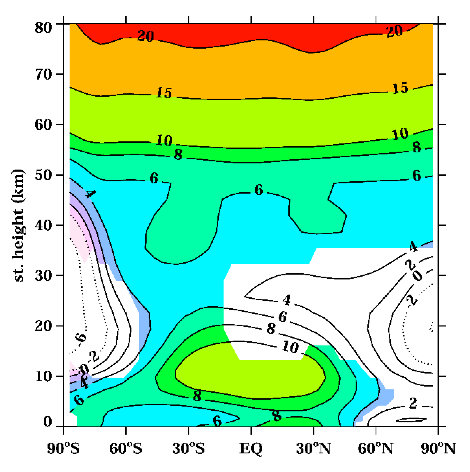
The active hydrogen oxides or HOx (OH + HO2) catalytically destroy ozone in the atmosphere. They are more effective in the lower and upper stratosphere [34]. Hydrogen oxides are produced from water vapor via photolysis by solar UV in the Lyman-α line and oxygen Schumann–Runge bands, or by reaction with exited atomic oxygen [33]. The solar activity modulates both factors because exited atomic oxygen is also produced by ozone photolysis. Water vapor depends on atmospheric transport and methane abundance, which are both modulated by natural and anthropogenic activities. The annual and zonal mean HOx trend is illustrated in Figure 1.
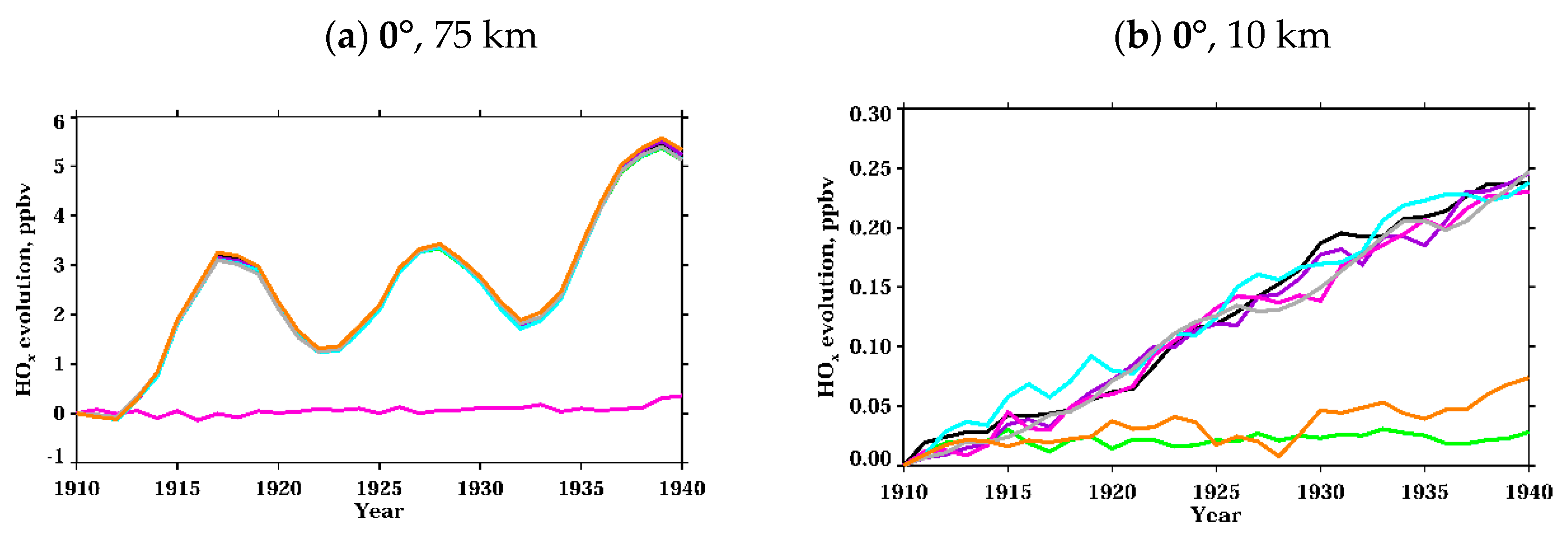
The HOx trend is most pronounced (more than 10%) above 50 km and in the tropical troposphere. To identify the drivers of such changes we show the evolution of the HOx mixing ratio in Figure 2 for these two regions.
Figure 2a shows that, in the upper atmosphere above 50 km, the influence of solar UV irradiance dominates, because for the fixUV model experiment the HOx mixing ratio does not change with time. For all other experiments, when the solar UV is not fixed, the HOx mixing ratio follows the behavior of solar activity. In the troposphere (Figure 2b), anthropogenic emissions play the most important role. The HOx increase is explained by enhanced water vapor in the warmer climate [19] and increased tropospheric ozone (Section 3.2). The direct sink of hydroxyl caused by enhanced methane and CO abundances is less important in the free troposphere, however, it almost completely eliminates the HOx increase over the Northern Hemisphere, where the intensification of anthropogenic carbon monoxide emissions is most pronounced.
3.1.2. Nitrogen Oxides
Nitrogen oxides or NOy (N + NO + NO2 + HNO3 + HNO4 + 2*N2O5) participate in catalytic ozone loss in the atmosphere. They are more effective in the middle stratosphere [34]. Nitrogen oxides are produced mostly from the N2O reaction with exited atomic oxygen [33]. The precipitating energetic particles also produce NOy over high latitudes during the winter season [35]. Solar activity modulates both factors because the concentration of exited atomic oxygen depends on ozone photolysis, and energetic particle precipitation depends on the solar wind. The main stratospheric loss of NOy is the cannibalistic reaction N + NO = N2 + O [33] driven by NO photolysis. The tropospheric NOy level strongly depends on anthropogenic activity [10]. The annual and zonal mean NOy trend is illustrated in Figure 3.
The NOy trend is most pronounced in the stratosphere, free northern troposphere, and polar mesosphere. The evolution of the NOy mixing ratio is illustrated in Figure 4 for two above-mentioned regions to identify the responsible forcing.
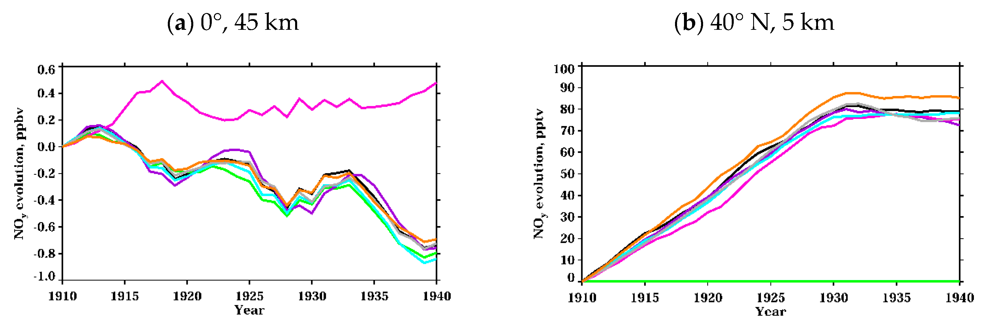
Figure 4a demonstrates that the influence of solar UV irradiance dominates in the stratosphere, because without the UV forcing the NOy mixing ratio only changes slightly with time. When the solar UV forcing is switched on, the behavior of the NOy mixing ratio resembles the solar activity evolution due to the NO photolysis modulation by the solar activity. In the troposphere, the anthropogenic emissions of NO and NO2 (NOx) play the most important role leading to the substantial (by up to 90 pptv) NOy increase. The results of the model run with fixed NOx emissions, shown by the green line in Figure 4b, demonstrate the absence of detectable NOy evolution when the anthropogenic emissions of NO and NO2 (NOx) are fixed. Weak changes in NOy after 1930 are related to a slower increase in anthropogenic NOx emissions [31]. The NOy increase in the mesosphere is fully defined by the increased intensity of energetic particle precipitation caused by stronger solar and geomagnetic activity (not shown).
3.1.3. Temperature
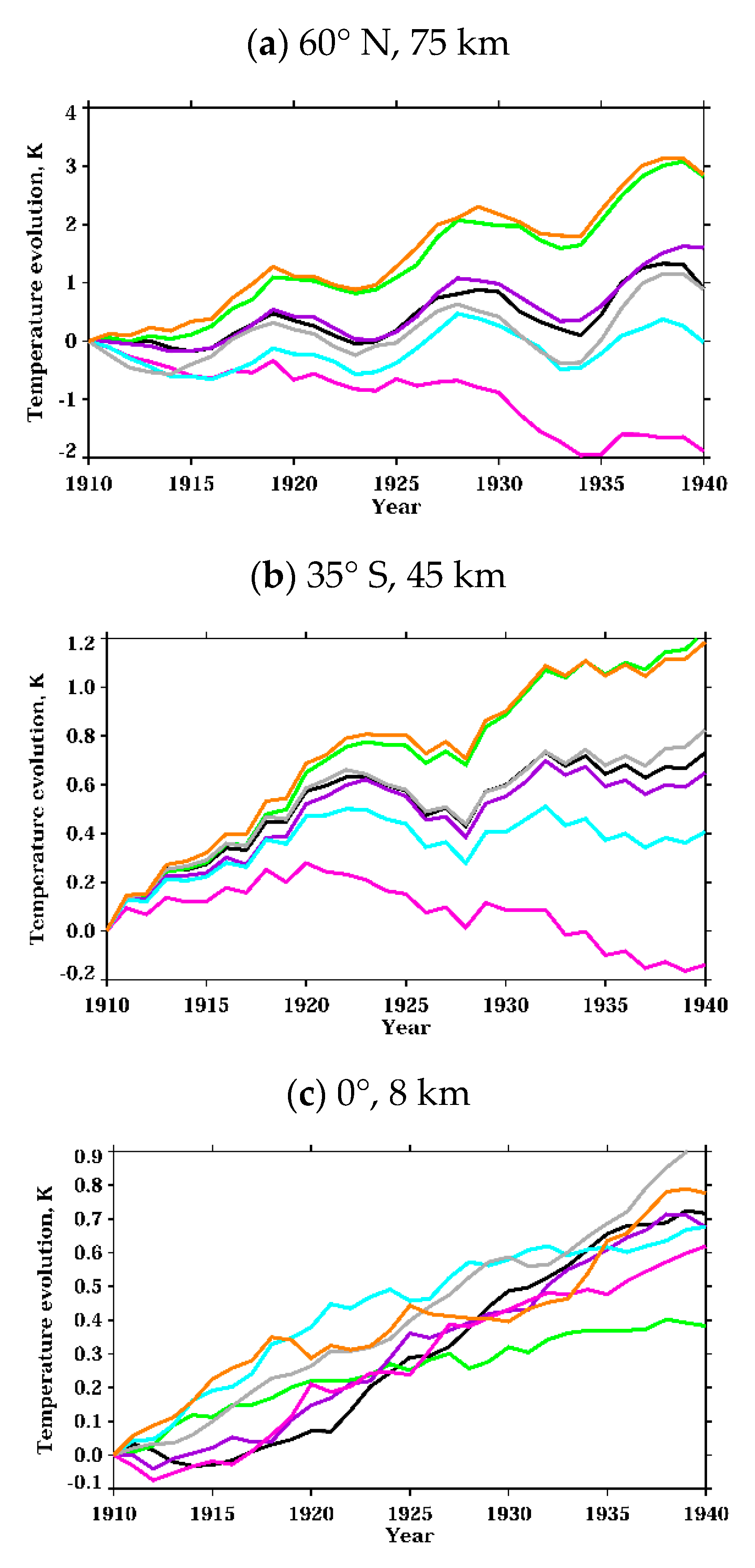
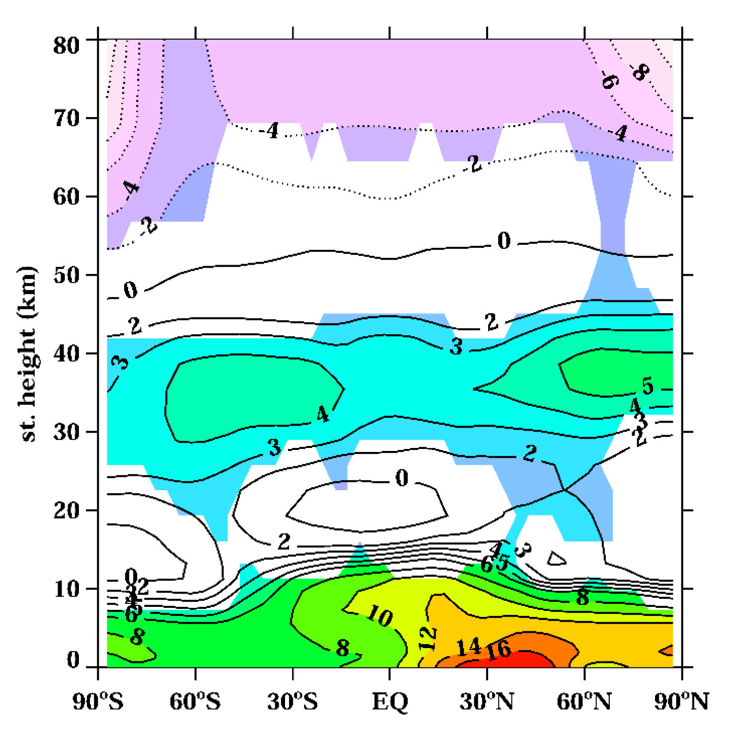
Temperature is important for the processes regulating ozone balance, because kinetic reaction rates are temperature dependent [33]. Atmospheric temperature depends on a multitude of physical and chemical processes driven by both natural and anthropogenic factors. Figure 5 demonstrates temperature changes during the 1910 to 1940 period.
A warming trend is visible in almost the entire atmosphere but is small and not statistically significant in the middle stratosphere. The troposphere becomes warmer, in 1940, by up to 0.6 K as compared with in 1910. The obtained surface warming was described in detail by [19]. They obtained about 0.4 K global mean warming defined mostly by well-mixed greenhouse gases (about 50%) and solar irradiance in the visible and near infrared parts of the spectrum (35%). Some contribution (about 15%) comes from the tropospheric ozone increase caused by ozone precursor emissions. Stronger warming (1 to 2 K) appears in the upper stratosphere and mesosphere. Two warming spots in the upper stratosphere over the northern and southern tropics have the same origin as in the mesosphere, but of a smaller magnitude. Over the equator the temperature changes are smaller and have only marginal significance because the solar UV forcing is less efficient in this area and does not completely dominate over the greenhouse gas forcing.
Figure 6 illustrates the contribution of different factors to the temperature evolution during the period considered. Warming in the mesosphere, for the case with all drivers switched on (black line), is formed by competition between solar UV irradiance heating and cooling by well-mixed greenhouse gases with a small contribution from solar irradiance in the visible spectral region (light blue line in Figure 6a). When the solar UV irradiance is fixed (magenta line in Figure 6a), greenhouse gases cools mesosphere down by up to 2 K. In the absence of greenhouse gas changes (green and orange curves in Figure 6a), the heating from the absorption of enhanced solar UV irradiance leads to a warming of the mesosphere by up to 3 K. In addition, variable solar UV irradiance effects are visible in decadal scale variability with the magnitude of 0.75 K from the solar activity cycle.
In the middle tropical troposphere, the analysis is rather complicated. Except the dominating contribution from tropospheric ozone precursors over well-mixed greenhouse gases (compare orange and green lines in Figure 6c), it is difficult to identify the most important factors.
3.2. Analysis of the Ozone Layer Evolution
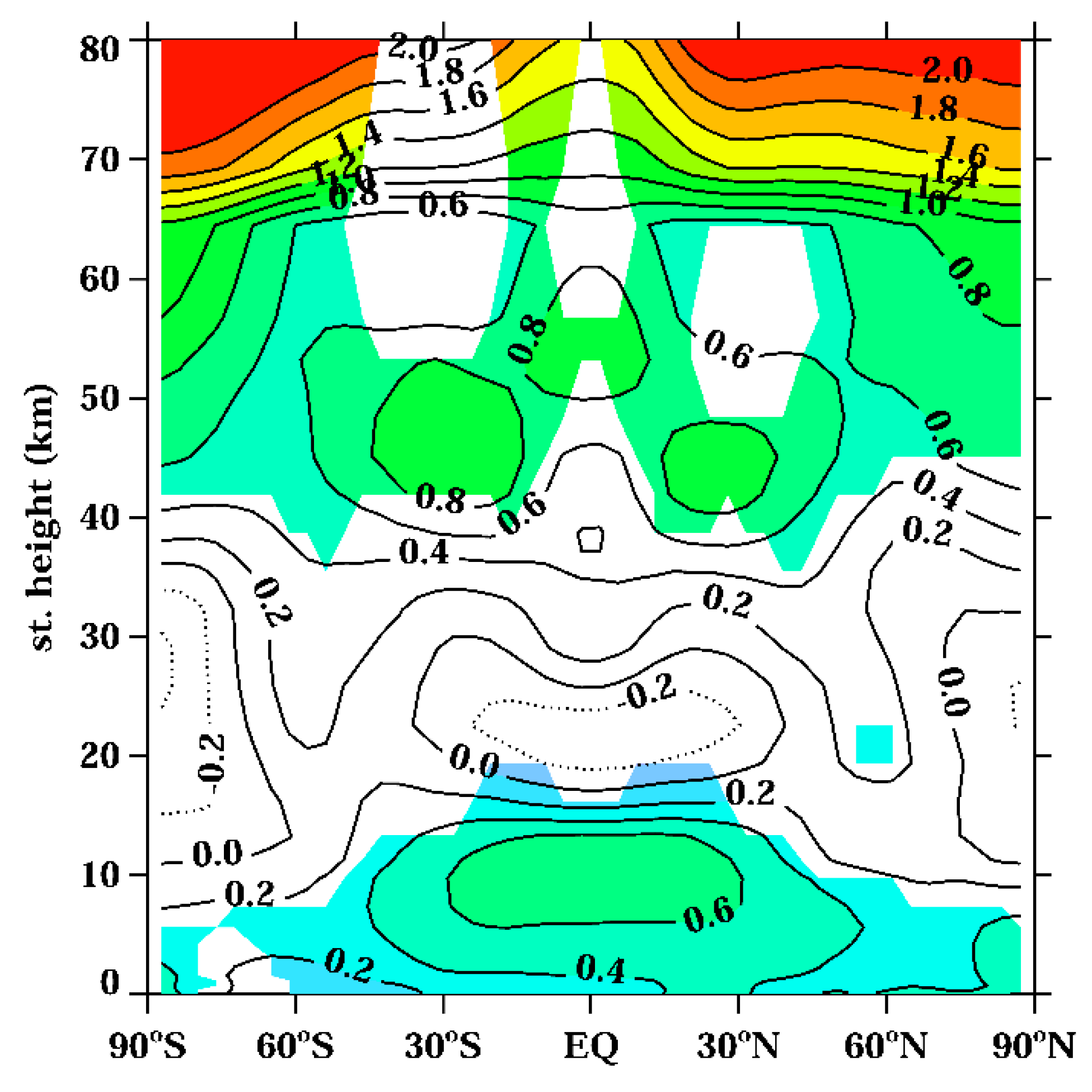
The ozone changes depend on all drivers considered in Section 3.1, as well as on the transport processes related to continuous climate warming during the considered period [19]. Figure 7 demonstrates the ozone changes between 1910 and 1940. The obtained results allow three major areas with different ozone behavior to be identified as follows: the mesosphere, the middle stratosphere, and the troposphere. Ozone depletion is visible in the entire mesosphere, with the maxima in the polar regions of up to 10%. The opposite effect occurs in the middle stratosphere and troposphere, where the ozone concentration increases up to 5% and 20%, respectively. In the lower and upper stratosphere ozone trends are small and statistically insignificant.
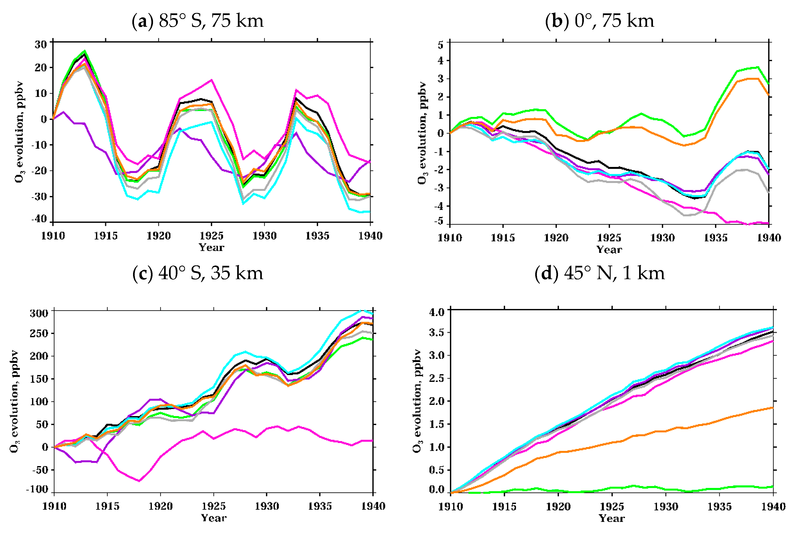
The time evolution of the annual zonal mean ozone mixing ratio and the contribution of different forcings for key altitude and latitude areas are shown in Figure 8. In the southern polar upper mesosphere (Figure 8a), the ozone evolution is reversed relative to solar activity for all experiments but has different magnitudes. The greatest contribution to the negative ozone trend in the mesosphere is related to the energetic particles, which produce more reactive hydrogen and nitrogen oxides during high solar and geomagnetic activity. The other drivers do not significantly affect the ozone evolution in this atmospheric region. The solar cycle is visible even in the absence of UV variability because the energetic particles forcing also has a decadal scale variability.
In the tropical mesosphere (Figure 8b) all drivers of ozone evolution can be separated into three groups. For the fixUV case, the ozone mixing ratio steadily decreases with time due to an increase in HOx (Figure 2) caused by an increase in the production of water vapor from enhanced methane emission. The cooling of the mesosphere caused by the increase in well-mixed greenhouse gases (see the discussion of Figure 6a) suppresses the intensity of the ozone destruction cycles and leads to a small ozone increase, however, it cannot compensate for the influence of HOx. The lack of a variable solar UV irradiance also explains the absence of cyclical ozone behavior which is visible for all other cases. For the fixGHG and fixWMGHG cases, the gradual ozone increase is driven mostly by the solar UV changes, which more than compensate for the HOx increase due to the enhanced H2O photolysis (Figure 2). Thus, the ozone evolution of the ALL experiment is formed from the competition between a greenhouse gas induced HOx increase and a solar UV irradiance enhancement.
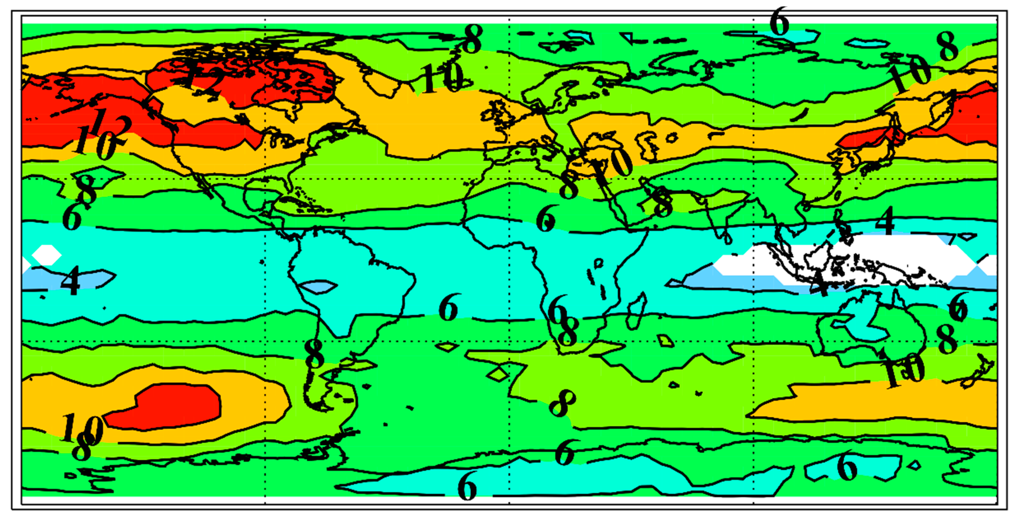
In the middle stratosphere over southern middle latitudes (Figure 8c), variations in solar UV irradiance play a dominant role that lead to a substantial increase in the ozone mixing ratio and almost constant values in the case when solar UV irradiance is fixed (case fixUV). In the lower troposphere over northern latitudes (Figure 8d), the ozone evolution is driven by tropospheric ozone precursors (fixGHG case) and, to a lesser extent, by the well-mixed greenhouse gases (fixWMGHG case). In the latter case, the ozone increase is related to enhanced methane emissions. The geographical distribution of the changes in annual mean total ozone from 1910 to 1940 driven by all considered forcing agents is illustrated in Figure 9. The simulated total ozone changes are positive and statistically significant all over the globe except in the western Pacific. In the tropical and high latitude belts, the changes are about 6 DU. More pronounced total column ozone trends are found over the middle latitudes in both hemispheres. There, the ozone change from 1910 to 1940.
The 1910 to 1940 time period from the run ALL, the area where the trend is significant at the 90% or better level, is marked by color shading and reaches 12 DU (about 4%) over North America, as well as over the northern and southern parts of the Pacific Ocean. Over Europe, the total ozone increase is slightly smaller but still exceeds 10 DU. These areas are typical locations of spring maxima in the total column ozone distribution caused by a spring-time acceleration of the meridional circulation transporting ozone down from its production area. Therefore, these changes in the total column ozone can be largely attributed to an increase in stratospheric production by enhanced solar UV irradiance. The contribution from tropospheric ozone is small because about 90% of the total column ozone is located in the stratosphere.
4. Discussion
Our results show the importance of an accurate prescription of both natural and anthropogenic forcings to reconstruct past climate and ozone layer trends. The estimate of the total column ozone trend during the first half of the 20th century, obtained by [15] using mostly anthropogenic forcing, does not exceed 1.0 DU. A consideration of the natural forcing by [16] led to the much higher value of almost 3.0 DU. In the present work, using new estimates for the solar forcing from [28], we obtained a three times stronger effect reaching almost 8 DU for the global annual mean value, and 12 DU over the northern and southern middle latitudes. The enhanced magnitude of the total column ozone changes is explained solely by the applied strong solar forcing. Thus, a poor understanding of the solar forcing automatically leads to large uncertainty in the simulated total ozone evolution. However, a high sensitivity of the total column ozone to solar UV forcing can be used to resolve long standing issues about the absolute value of the magnitude of past solar irradiance variability discussed recently by [17]. This problem can potentially be solved by comparing the simulated total ozone behavior with direct measurements or proxy-based reconstructions. Unfortunately, direct comparisons of simulated and observed total column ozone trends is not possible from 1910 to 1940 because the observations are available only from 1926 [36]. The proxy-based reconstructions of total ozone are not available at the moment, but there is some progress in this direction. One possible approach is to retrieve surface UV-B radiation level at the surface from the analysis of UV-B absorbing objects in the plants or spores [37,38,39,40]. However, it is not clear how to separate the influence of stratospheric ozone variations from the spectral solar irradiance variability, which is not well constraint on long-term time scales [17]. The simulated changes in the total column ozone are mainly caused by the ozone evolution in the middle stratosphere driven by steadily growing extraterrestrial solar UV irradiance. The simulated shape of the stratospheric ozone increase, shown in Figure 7, resembles the ozone response to the solar UV irradiance enhancement during the recent period [40] only in the tropical middle stratosphere (between 30 and 40 km). The elevated secondary ozone enhancement in the upper stratosphere over midlatitudes obtained by [40] from observations and model simulations are not visible in our results. The difference can be explained by different circulation regimes in these two periods. A possible influence from the circulation is illustrated in [40] from a comparison of free running and specified dynamics model runs. In the case of a free running model, the upper stratospheric spots of enhanced ozone are much less pronounced in comparison with specified dynamics runs. This difference should be related to different circulation fields, because the treatment of chemical and transport processes is identical in both model versions.
An accurate knowledge of the tropospheric ozone evolution is also important, because it can play an important role in the explanation of the early 20th century warming (ETCW). It was shown in [19] that tropospheric ozone precursors (CO and NOx) are the third most important factor influencing climate during this period, after greenhouse gases, solar visible, and infrared radiation. Therefore, an underestimation of the CO and NOx emission intensification can explain an underestimation of the ETCW magnitude in many climate models [18]. The simulated annual mean tropospheric ozone mixing ratio in 1910 varies between 15 and 30 ppb over the northern mid-latitudes depending on the location and season, which overestimates 10 to 15 ppb obtained from direct surface ozone measurements at different locations in central Europe [6,10]. It should be noted, however, that these historical measurements probably underestimate ozone mixing ratios due to interference from water vapor and other species [41]. The subsequent ozone increase (Figure 7 and Figure 8d) of about 4 ppb (~15%) during 1910 to 1940, in our experiment, is close to the 11% increase simulated by [10], and 16% obtained from direct ozone measurements at mountain sites [5]. Our simulations of the rate of the tropospheric ozone increase agree with the isotope analysis of air trapped in the ice and snow, as well as with results from the GISS-E2.1 model [41].
The presented analysis can be extended to cover trends of halogenated species and atmospheric dynamics. We do not expect substantial contributions from the halogenated species because of their very small (more than six times as compare with present day) abundance and absence of trends during the considered period. Dynamical changes caused by climate warming could consist of an altered tropopause height, state of the polar vortices, or Brewer–Dobson circulation (BDC) intensity. However, the analysis of their trends is more difficult because the response of dynamical properties has a low signal-to-noise ratio. For example, the lower stratospheric ozone depletion in the tropical area caused by enhanced BDC in a warmer climate, and clearly visible in the simulation of the future climate [42], is not significant in our case (Figure 7). The same can be said about the dipole-like polar temperature changes which characterize polar vortex strengthening (Figure 5). Probably, these changes should be examined in the future on seasonal or even monthly time scales.
5. Conclusions
In this study of ozone layer evolution during the early 20th century, we exploited the chemistry-climate model SOCOL-MPIOM driven by all known anthropogenic and natural forcing agents, as well as their combinations. Using results from seven ten-member ensemble runs, we demonstrate the time evolution of the main factors responsible for t ozone production and loss from the ground to the mesopause. We demonstrate that in the mesosphere the ozone mixing ratio trend during the 1910 to 1940 period is negative and driven by energetic particles, incoming solar UV radiation, and greenhouse gases. In the middle stratosphere, the ozone increased from 1910 to 1940 by up to 5%, mostly due to the enhancement of solar UV radiation.
Our calculations emphasize the dominant role of anthropogenic factors in the troposphere, where an increase in CO and NOx emissions leads to an increase in ozone mixing ratios by up to 15%. The general agreement of the increase in tropospheric ozone with previously published estimates allows us to conclude that a climate influence from this forcing is rather well constrained and cannot explain the underprediction of the ETCW magnitude by many climate models [18,19].
We obtained a significant global scale increase in the total column ozone exceeding 12 Dobson Units over northern and southern middle latitudes. We conclude that total column ozone changes during this period were driven mostly by an enhancement in solar UV radiation. Our simulation results can be used to constrain the solar forcing magnitude if past ozone or solar UV-B radiation becomes available.
Author Contributions
Data curation, T.S.; Software, P.A.; Supervision, E.R.; Writing – original draft, T.E. All authors have read and agreed to the published version of the manuscript.
Funding
This research was funded by the Swiss National Science Foundation under grants CRSII2-147659 (FUPSOL-II) and 200020_182239 (POLE).
Acknowledgments
Numerical simulations were performed on the ETH Zürich cluster EULER. Our special thanks to W. Ball for the English grammar improvement.
Conflicts of Interest
The authors declare no conflict of interest.
References
- Bais, A.F.; Lucas, R.M.; Bornman, J.F.; Williamson, C.E.; Sulzberger, B.; Austin, A.T.; Wilson, S.R.; Andrady, A.L.; Bernhard, G.; McKenzie, R.L.; et al. Environmental effects of ozone depletion, UV radiation and interactions with climate change: UNEP Environmental Effects Assessment Panel, update 2017. Photochem. Photobiol. Sci. 2018, 17, 127–179. [Google Scholar] [CrossRef] [PubMed]
- Häder, D.-P.; Barnes, P.W. Comparing the impacts of climate change on the responses and linkages between terrestrial and aquatic ecosystems. Sci. Total Environ. 2019, 682, 239–246. [Google Scholar] [CrossRef] [PubMed]
- WMO (World Meteorological Organization). Scientific Assessment of Ozone Depletion: 2018; Global Ozone Research and Monitoring Project—Report No. 58; WMO: Geneva, Switzerland, 2018; 588p. [Google Scholar]
- Volz, A.; Kley, D. Evaluation of the Montsouris series of ozone measurements made in the nineteenth century. Nature 1988, 332, 240–242. [Google Scholar] [CrossRef]
- Marenco, A.; Gouget, H.; Nedelec, P.; Pages, J.-P. Evidence of a long-term increase in tropospheric ozone from Pic du Midi data series: Consequences: Positive radiative forcing. J. Geophys. Res. 1994, 99, 16617–16632. [Google Scholar] [CrossRef]
- Hauglustaine, D.A.; Brasseur, G.P. Evolution of tropospheric ozone under anthropogenic activities and associated radiative forcing of climate. J. Geophys. Res. 2001, 106, 32337–32360. [Google Scholar] [CrossRef] [Green Version]
- Chalita, S.; Hauglustaine, D.A.; Letreut, H.; Müller, J.-F. Radiative forcing due to increased tropospheric ozone concentrations. Atmos. Environ. 1996, 30, 1641–1646. [Google Scholar] [CrossRef]
- Mickley, L.J.; Jacob, D.J.; Rind, D. Uncertainty in preindustrial abundance of tropospheric ozone: Implications for radiative forcing calculations. J. Geophys. Res. 2001, 106, 3389–3399. [Google Scholar] [CrossRef]
- Shindell, D.T.; Faluvegi, G.; Bell, N. Preindustrial-to-present-day radiative forcing by tropospheric ozone from improved simulations with the GISS chemistry-climate GCM. Atmos. Chem. Phys. 2003, 3, 1675–1702. [Google Scholar] [CrossRef] [Green Version]
- Lamarque, J.-F.; Hess, P.; Emmons, L.; Buja, L.; Washington, W.; Granier, C. Tropospheric ozone evolution between 1890 and 1990. J. Geophys. Res. 2004, 110, D08304. [Google Scholar] [CrossRef]
- Parrella, J.P.; Jacob, D.J.; Liang, Q.; Zhang, Y.; Mickley, L.J.; Miller, B.F.; Evans, M.J.; Yang, X.; Pyle, J.A.; Theys, N.; et al. Tropospheric bromine chemistry: implications for present and pre-industrial ozone and mercury. Atmos. Chem. Phys. 2012, 12, 6723–6740. [Google Scholar] [CrossRef] [Green Version]
- Young, P.J.; Archibald, A.T.; Bowman, K.W.; Lamarque, J.-F.; Naik, V.; Stevenson, D.S.; Tilmes, S.; Voulgarakis, A.; Wild, O.; Bergmann, D. Pre-industrial to end 21st century projections of tropospheric ozone from the Atmospheric Chemistry and Climate Model Intercomparison Project (ACCMIP). Atmos. Chem. Phys. 2013, 13, 2063–2090. [Google Scholar] [CrossRef] [Green Version]
- Reader, M.C.; Plummer, D.A.; Scinocca, J.F.; Shepherd, T.G. Contributions to twentieth century total column ozone change from halocarbons, tropospheric ozone precursors, and climate change. Geophys. Res. Lett. 2013, 40, 6276–6281. [Google Scholar] [CrossRef] [Green Version]
- Hollaway, M.J.; Arnold, S.R.; Collins, W.J.; Folberth, G.; Rap, A. Sensitivity of midnineteenth century tropospheric ozone to atmospheric chemistry-vegetation interactions. Geophys. Res. Atmos. 2011, 122, 2452–2473. [Google Scholar] [CrossRef] [Green Version]
- Fleming, E.L.; Jackman, C.H.; Stolarski, R.S.; Douglass, A.R. A model study of the impact of source gas changes on the stratosphere for 1850–2100. Atmos. Chem. Phys. 2011, 11, 8515–8541. [Google Scholar] [CrossRef] [Green Version]
- Lean, J. Evolution of Total Atmospheric Ozone from 1900 to 2100 Estimated with Statistical Models. J. Atmos. Sci. 2014, 71, 1956–1984. [Google Scholar] [CrossRef]
- Egorova, T.; Schmutz, W.; Rozanov, E.; Shapiro, A.I.; Usoskin, I.; Beer, J.; Tagirov, R.V.; Peter, T. Revised historical solar irradiance forcing. Astron. Astrophys. 2018, 615, A85. [Google Scholar] [CrossRef] [Green Version]
- Hegerl, G.C.; Brönnimann, S.; Schurer, A.; Cowan, T. The early 20th century warming: anomalies, causes, and consequences. WIREs Clim. Chang. 2018, 9, e522. [Google Scholar] [CrossRef] [Green Version]
- Egorova, T.; Rozanov, E.; Arsenovic, P.; Peter, T.; Schmutz, W. Contributions of Natural and Anthropogenic Forcing Agents to the Early 20th Century Warming. Front. Earth Sci. 2018, 6, 206. [Google Scholar] [CrossRef]
- Muthers, S.; Anet, J.G.; Stenke, A.; Raible, C.C.; Rozanov, E.; Brönnimann, S.; Peter, T.; Arfeuille, F.X.; Shapiro, A.I.; Beer, J.; et al. The coupled atmosphere-chemistry-ocean model SOCOL MPIOM. Geosci. Model. Dev. 2014, 7, 2157–2179. [Google Scholar] [CrossRef] [Green Version]
- Arsenovic, P.; Rozanov, E.; Anet, J.; Stenke, A.; Peter, T. Implications of potential future grand solar minimum for ozone layer and climate. Atmos. Chem. Phys. 2018, 18, 3469–3483. [Google Scholar] [CrossRef] [Green Version]
- Stenke, A.; Schraner, M.; Rozanov, E.; Egorova, T.; Luo, B.; Peter, T. The SOCOL version 3.0 chemistry–climate model: description, evaluation, and implications from an advanced transport algorithm. Geosci. Model. Dev. 2013, 6, 1407–1427. [Google Scholar] [CrossRef] [Green Version]
- Roeckner, E.; Bäuml, G.; Bonaventura, L.; Brokopf, R.; Esch, M.; Giorgetta, M.; Hagemann, S.; Kirchner, I.; Kornblueh, L.; Manzini, E.; et al. The Atmospheric General Circulation Model ECHAM5. Part I: Model Description; Report No. 349; Max Planck Institute for Meteorology: Hamburg, Germany, 2003. [Google Scholar]
- Rozanov, E.V.; Zubov, V.; Schlesinger, M.E.; Yang, F.; Andronova, N.G. The UIUC three-dimensional stratospheric chemical transport model: description and evaluation of the simulated source gases and ozone. J. Geophys. Res. 1999, 104, 11755–11781. [Google Scholar] [CrossRef]
- Egorova, T.; Rozanov, E.; Zubov, V.; Karol, I. Model for investigating ozone trends (MEZON). Izv. Atmos. Ocean. Phys. 2003, 39, 277–292. [Google Scholar]
- Marsland, S.J.; Haak, H.; Jungclaus, J.H.; Latif, M. The Max-Planck-Institute global ocean/sea ice model with orthogonal curvilinear coordinates. Ocean Model. 2003, 5, 91–127. [Google Scholar] [CrossRef] [Green Version]
- Jungclaus, J.H.; Keenlyside, N.; Botzet, M.; Haak, H.; Luo, J.-J.; Latif, M.; Marotzke, J.; Mikolajewicz, U.; Roeckner, E. Ocean Circulation and Tropical Variability in the Coupled Model ECHAM5/MPI-OM. J. Clim. 2006, 19, 3952–3972. [Google Scholar] [CrossRef] [Green Version]
- Shapiro, A.I.; Schmutz, W.; Rozanov, E.; Schoell, M.; Haberreiter, M.; Shapiro, A.V.; Nyeki, S. A new approach to the long-term reconstruction of the solar irradiance leads to large historical solar forcing. Astron. Astrophys. 2011, 529, A67. [Google Scholar] [CrossRef] [Green Version]
- Sukhodolov, T.; Rozanov, E.; Shapiro, A.I.; Anet, J.; Cagnazzo, C.; Peter, T.; Schmutz, W. Evaluation of the ECHAM family radiation codes performance in representation of the solar signal. Geosci. Model. Dev. 2014, 7, 2859–2866. [Google Scholar] [CrossRef] [Green Version]
- Matthes, K.; Funke, B.; Andersson, M.E.; Barnard, L.; Beer, J.; Charbonneau, P.; Clilverd, M.A.; de Wit, T.D.; Haberreiter, M.; Hendry, A.; et al. Solar forcing for CMIP6 (v3. 2). Geosci. Model. Dev. 2017, 10, 2247–2302. [Google Scholar] [CrossRef] [Green Version]
- Meinshausen, M.; Smith, S.J.; Calvin, K.; Daniel, J.S.; Kainuma, M.L.T.; Lamarque, J.-F.; Matsumoto, K.; Montzka, S.A.; Raper, S.C.B.; Riahi, K.; et al. The RCP greenhouse gas concentrations and their extensions from 1765 to 2300. Clim. Chang. 2011, 109, 213–241. [Google Scholar] [CrossRef] [Green Version]
- Gray, L.J.; Beer, J.; Geller, M.; Haigh, J.D.; Lockwood, M.; Matthes, K.; Cubasch, U.; Fleitmann, D.; Harrison, R.G.; Hood, L.; et al. Solar influence on climate. Rev. Geophys. 2010, 48, RG4001. [Google Scholar] [CrossRef]
- Brasseur, G.P.; Solomon, S. Aeronomy of the Middle Atmosphere: Chemistry and Physics of the Stratosphere and Mesosphere; Springer: Dordrecht, The Netherlands, 2005; Volume 32, p. 646. [Google Scholar] [CrossRef]
- Larin, I. On the chain length and rate of ozone depletion in the main stratospheric cycles. Atmos. Clim. Sci. 2013, 3, 141–149. [Google Scholar] [CrossRef] [Green Version]
- Mironova, I.A.; Aplin, K.L.; Arnold, F.; Bazilevskaya, G.A.; Harrison, R.G.; Krivolutsky, A.A.; Nicoll, K.A.; Rozanov, E.V.; Turunen, E.; Usoskin, I.G. Energetic Particle Influence on the Earth’s Atmosphere. Space Sci. Rev. 2015, 194, 1–96. [Google Scholar] [CrossRef] [Green Version]
- Scarnato, B.; Staehelin, J.; Stübi, R.; Schill, H. Long-term total ozone observations at Arosa (Switzerland) with Dobson and Brewer instruments (1988–2007). J. Geophys. Res. 2010, 115, D13306. [Google Scholar] [CrossRef] [Green Version]
- Rozema, J.; van Geel, B.; Bjorn, L.O.; Lean, J.; Madronich, S. PALEOCLIMATE: Toward Solving the UV Puzzle. Science 2002, 296, 1621–1622. [Google Scholar] [CrossRef] [Green Version]
- Magri, D. Past UV-B flux from fossil pollen: Prospects for climate, environment and evolution. New Phytol. 2011, 192, 310–312. [Google Scholar] [CrossRef] [PubMed] [Green Version]
- Jardine, P.E.; Fraser, W.T.; Gosling, W.D.; Roberts, C.N.; Eastwood, W.J.; Lomax, B.H. Proxy reconstruction of ultraviolet-B irradiance at the Earth’s surface, and its relationship with solar activity and ozone thickness. Holocene 2019. [Google Scholar] [CrossRef]
- Ball, W.T.; Rozanov, E.; Alsing, J.; Marsh, D.R.; Tummon, F.; Mortlock, D.J.; Kinnison, D.; Haigh, J.D. The upper stratospheric solar cycle ozone response. Geophys. Res. Lett. 2019, 46, 1831–1841. [Google Scholar] [CrossRef] [Green Version]
- Yeung, L.Y.; Murray, L.T.; Martinerie, P.; Witrant, E.; Hu, H.; Banerjee, A.; Orsi, A.; Chappellaz, J. Isotopic constraint on the twentieth-century increase in tropospheric ozone. Nature 2019, 570, 224–227. [Google Scholar] [CrossRef]
- Zubov, V.; Rozanov, E.; Egorova, T.; Karol, I.; Schmutz, W. Role of external factors in the evolution of the ozone layer and stratospheric circulation in 21st century. Atmos. Chem. Phys. 2013, 13, 4697–4706. [Google Scholar] [CrossRef] [Green Version]
Figure 1.
The annual and zonal mean HOx linear trend (%/31 years) during the 1910 to 1940 period for the ALL experiment. The area where the trend is significant at the 90% or better level is marked by color shading.
Figure 1.
The annual and zonal mean HOx linear trend (%/31 years) during the 1910 to 1940 period for the ALL experiment. The area where the trend is significant at the 90% or better level is marked by color shading.

Figure 2.
The time evolution of annual and zonal mean HOx since 1910. (a) In the tropical upper mesosphere panel; and (b) in the equatorial middle troposphere panel. The lines are black for ALL, violet for noEPP, magenta for fixUV, light blue for fixVIS/IR, green for fixGHG, orange for fixWMGHG, and grey for noVOL experiments.

Figure 3.
The annual and zonal mean NOy linear trend (%/31 years) during the 1910 to 1940 period for the ALL experiment. The area where the trend is significant at the 90% or better level is marked by color shading.
Figure 3.
The annual and zonal mean NOy linear trend (%/31 years) during the 1910 to 1940 period for the ALL experiment. The area where the trend is significant at the 90% or better level is marked by color shading.

Figure 4.
The evolution of annual and zonal mean NOy since 1910. (a) In the tropical upper stratosphere panel; (b) in the lower troposphere over northern midlatitudes panel. The lines are black for ALL, violet for noEPP, magenta for fixUV, light blue for fixVIS/IR, green for fixGHG, orange for fixWMGHG, and grey for noVOL experiments.

Figure 5.
The annual and zonal mean temperature linear trend (K/31 years) during the 1910 to 1940 period for the ALL experiment. The area where the trend is significant at the 90% or better level is marked by color shading.
Figure 5.
The annual and zonal mean temperature linear trend (K/31 years) during the 1910 to 1940 period for the ALL experiment. The area where the trend is significant at the 90% or better level is marked by color shading.

Figure 6.
The evolution of annual and zonal mean temperature since the 1910. (a) In the northern midlatitude mesosphere panel; (b) in the upper stratosphere over southern midlatitudes panel; and (c) in the tropical middle troposphere panel. The lines are black for ALL, violet for noEPP, magenta for fixUV, light blue for fixVIS/IR, green for fixGHG, orange for fixWMGHG, and grey for noVOL experiments.

Figure 7.
The annual and zonal mean ozone linear trend (%/31 years) during 1910 to 1940 for the ALL experiment. The area where the trend is significant at the 90% or better level is marked by color shading.
Figure 7.
The annual and zonal mean ozone linear trend (%/31 years) during 1910 to 1940 for the ALL experiment. The area where the trend is significant at the 90% or better level is marked by color shading.

Figure 8.
The evolution of annual zonal mean ozone mixing ratios since 1910. (a) In the southern polar upper mesosphere panel; (b) in the tropical mesosphere panel; (c) in the middle stratosphere over southern midlatitudes panel; and (d) in the the lower troposphere over northern midlatitudes panel. The lines are black for ALL, violet for noEPP, magenta for fixUV, light blue for fixVIS/IR, green for fixGHG, orange for fixWMGHG, and grey for noVOL experiments.

Figure 9.
Geographical distribution of the annual mean total column ozone trend (DU/31 years) during.
Figure 9.
Geographical distribution of the annual mean total column ozone trend (DU/31 years) during.


Table 1.
The list of performed ensemble numerical experiments.
| Experiment Name | Fixed Forcing | Color Code for Evolution Plots |
|---|---|---|
| ALL | None | Black |
| noEPP | Energetic particles | Violet |
| fixUV | Solar UV irradiance (λ < 250 nm), extra heating, and photolysis rates | Magenta |
| fixVIS/IR | Solar visible and near infrared irradiance | Light blue |
| fixGHG | CO2, N2O, CH4, NOx, and CO emissions | Green |
| fixWMGHG | CO2, N2O, and CH4 | Orange |
| noVOL | Stratospheric sulfate aerosol | Grey |
© 2020 by the authors. Licensee MDPI, Basel, Switzerland. This article is an open access article distributed under the terms and conditions of the Creative Commons Attribution (CC BY) license (http://creativecommons.org/licenses/by/4.0/).
Share and Cite
MDPI and ACS Style
Egorova, T.; Rozanov, E.; Arsenovic, P.; Sukhodolov, T. Ozone Layer Evolution in the Early 20th Century. Atmosphere 2020, 11, 169. https://0-doi-org.brum.beds.ac.uk/10.3390/atmos11020169
AMA Style
Egorova T, Rozanov E, Arsenovic P, Sukhodolov T. Ozone Layer Evolution in the Early 20th Century. Atmosphere. 2020; 11(2):169. https://0-doi-org.brum.beds.ac.uk/10.3390/atmos11020169
Chicago/Turabian StyleEgorova, Tatiana, Eugene Rozanov, Pavle Arsenovic, and Timofei Sukhodolov. 2020. "Ozone Layer Evolution in the Early 20th Century" Atmosphere 11, no. 2: 169. https://0-doi-org.brum.beds.ac.uk/10.3390/atmos11020169
Note that from the first issue of 2016, this journal uses article numbers instead of page numbers. See further details here.