Application of Data Fusion Techniques to Improve Air Quality Forecast: A Case Study in the Northern Italy


Abstract
:1. Introduction
- Off-line re-analysis techniques, performing an ex-post integration of the measurements with the model results, once they are computed. Off-line techniques usually include statistical methodologies: optimal interpolation methods [23], kriging and cokriging techniques [24,25]. These techniques allow, for example, the computing of reanalyzed spatial concentration fields or, in the forecasting applications, the best known estimate of the initial condition for the next day/hour [26]. In [27] a bias correction technique is presented showing a good increase in the forecasting performances for PM, ozone and nitrogen oxides.
- On-line data assimilation techniques fully integrate the impact of the measurements directly inside the model during the simulation. They can include variational methods (2D-, 3D, 4D-var) aimed at minimizing the distance between estimated concentration and observed data ([28]) or ensemble methodologies mainly applied for ozone or nitrogen dioxide concentrations [29,30]. The main drawback of these approaches is that their implementation usually needs strong changes in the core model code [21].
2. Materials and Methods
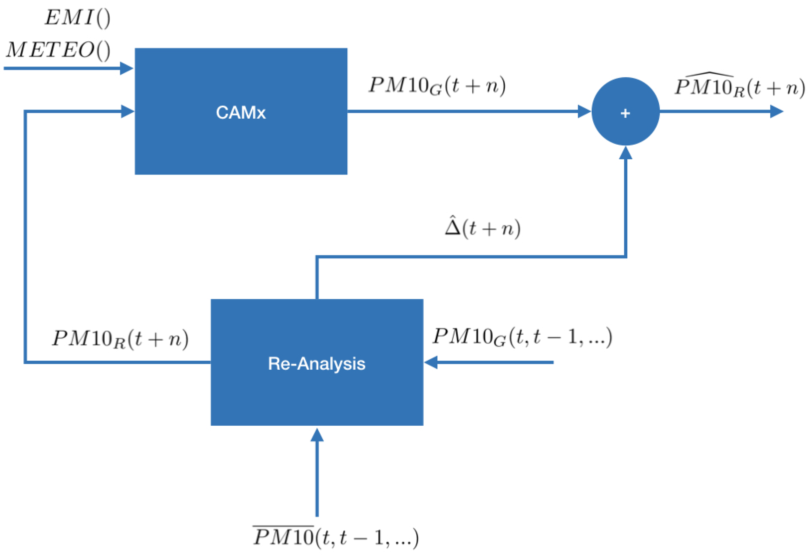
- setup of the best initial condition () for the forecast;
- estimation of the correction () for the forecasting steps ;
- application of estimated correction to the forecast computed by CAMx model .
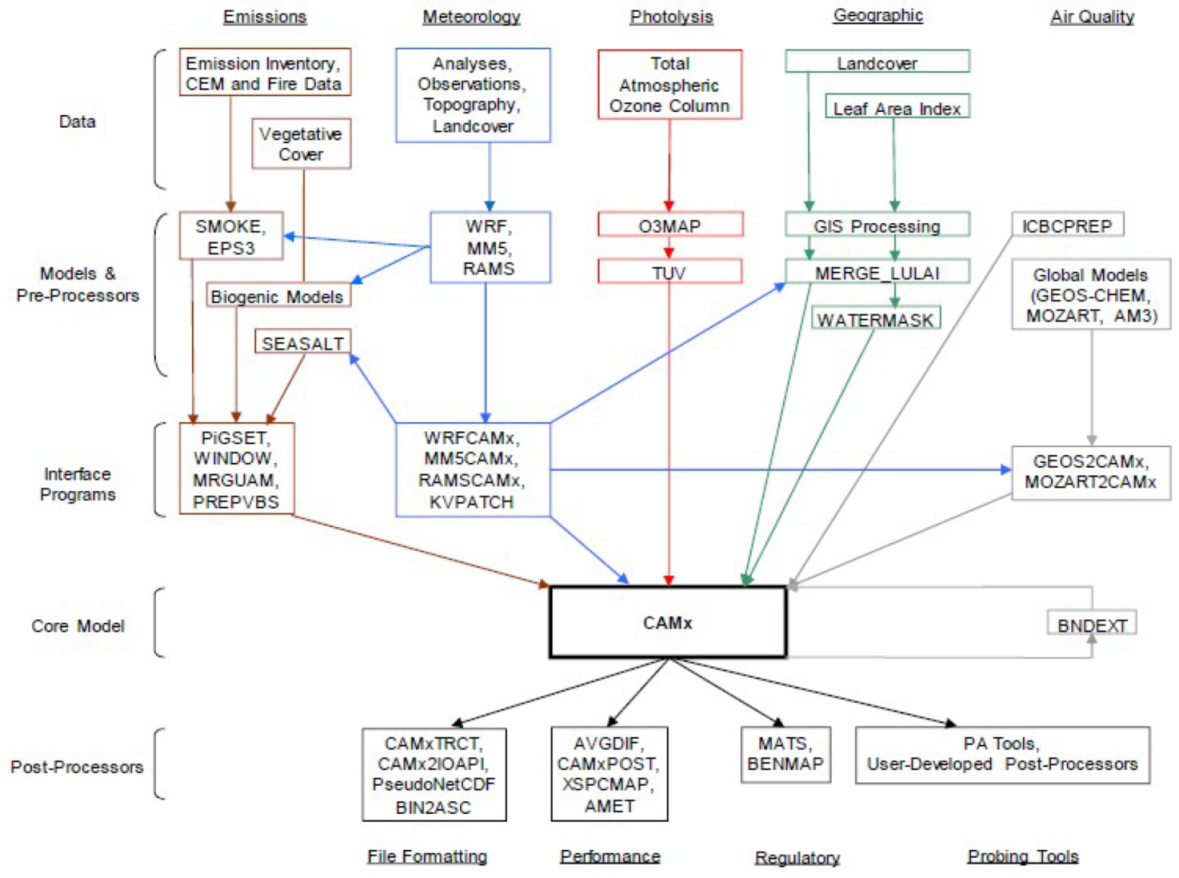
2.1. CAMx Model
- gridded and point source emission data;
- meteorology defined through the use of prognostic meteorological models (for example WRF [34]);
- photolysis rates for the photochemical mechanism;
- land cover information;
- boundary conditions are available from global models.
2.1.1. Re-analysis Phase
2.1.2. Optimal Interpolation
- is the re-analyzed PM10 fields at time t;
- is the background field at time t, i.e., the output of CAMx model before integration with the measurements;
- are the (pointwise) measurements of PM10 at monitoring station locations;
- H is a mathematical operator allowing to extract the background concentrations at the monitoring locations.
- is a matrix gain, often called Kalman gain, computed in order to minimize the variance of the errors.
2.1.3. Weighted Mean Approach
2.1.4. Least-square Error Approach
- Collecting all the , ;
- Defining the output matrix including the values of for each cell of the domain at time (last available);
- Defining the input matrix including for the first m columns the value of for each cell of the domain at time , and as a last column a vector of value equal to 1, in order to compute the depolarization term ().
- Applying the least square Equation ((8)) for linear parameter models:
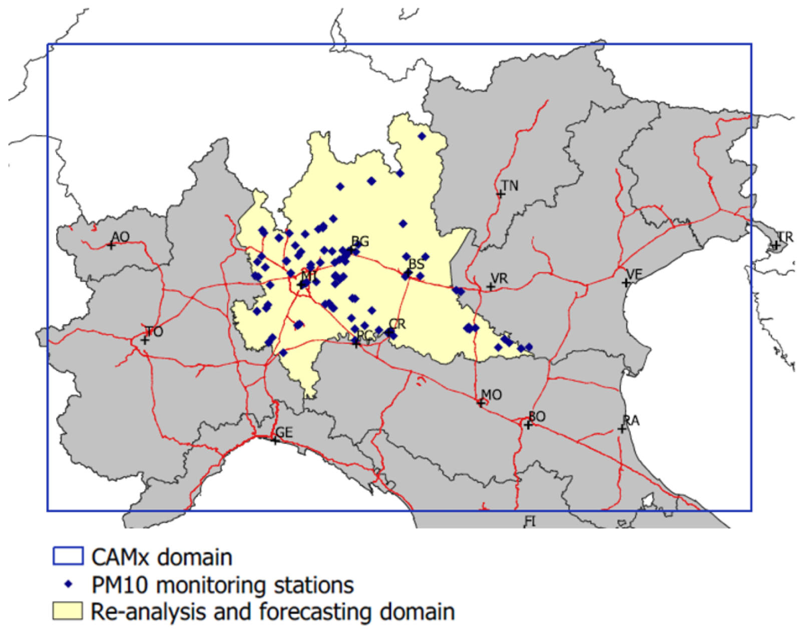
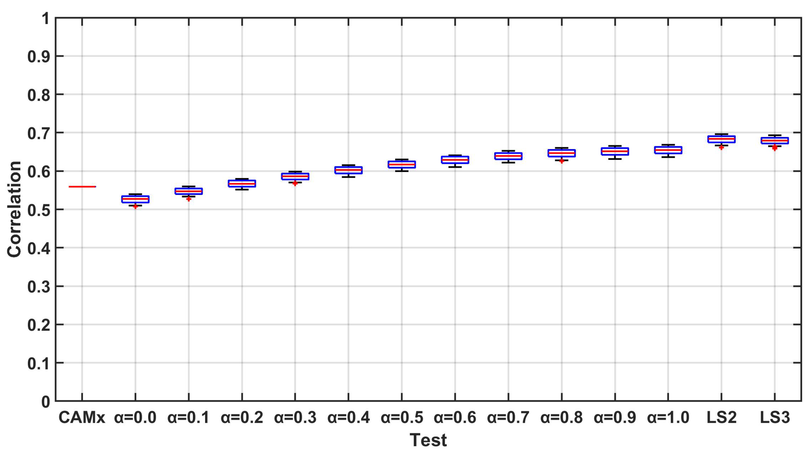
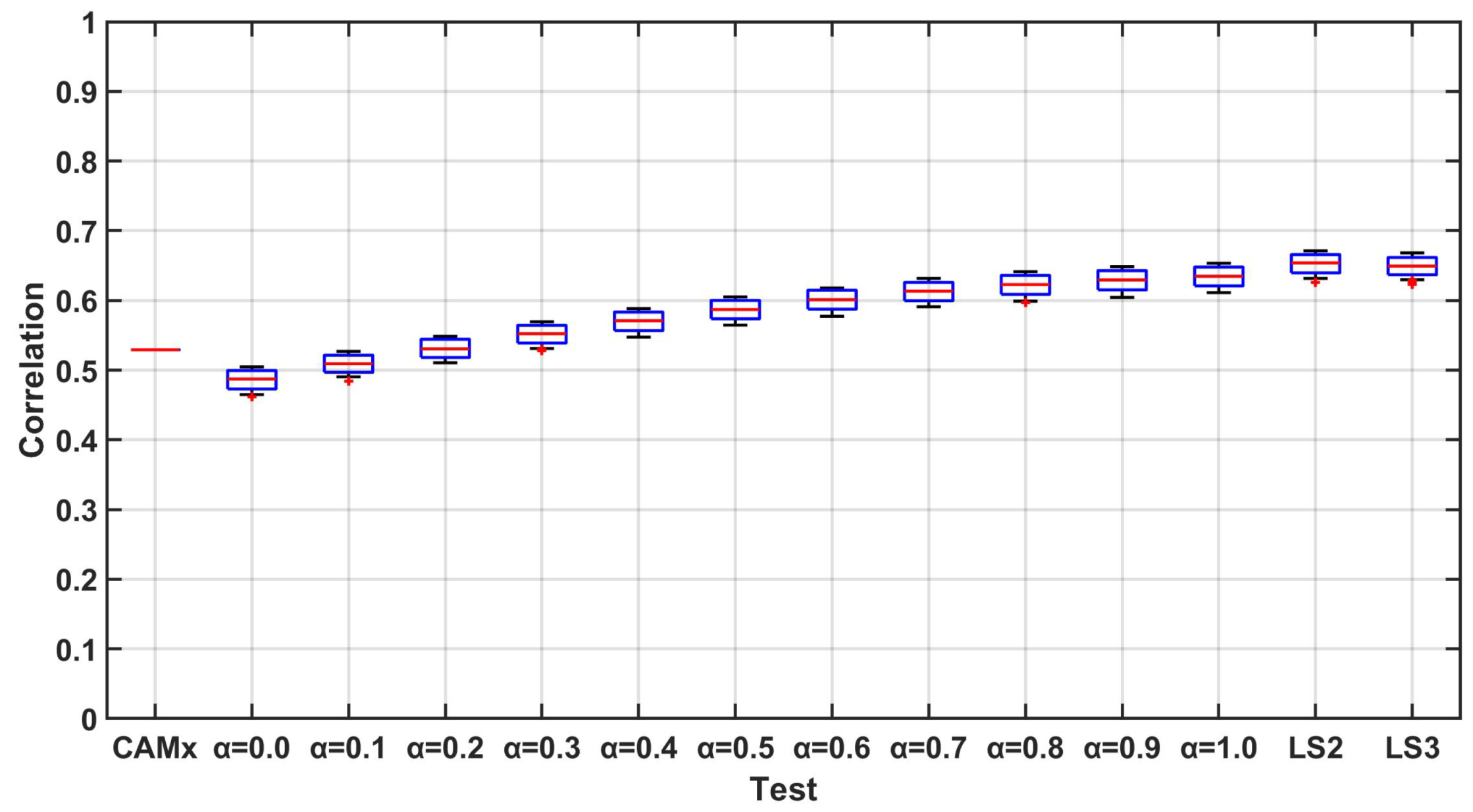
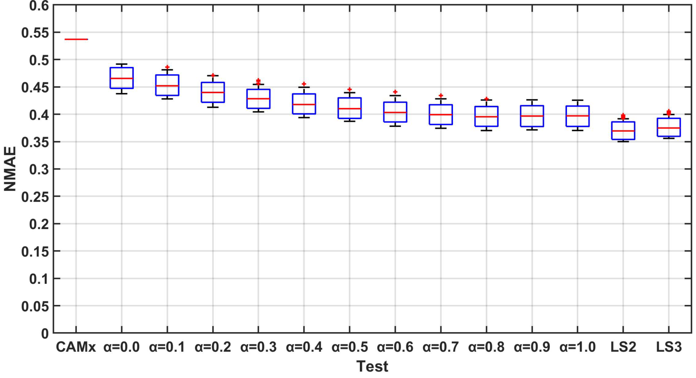
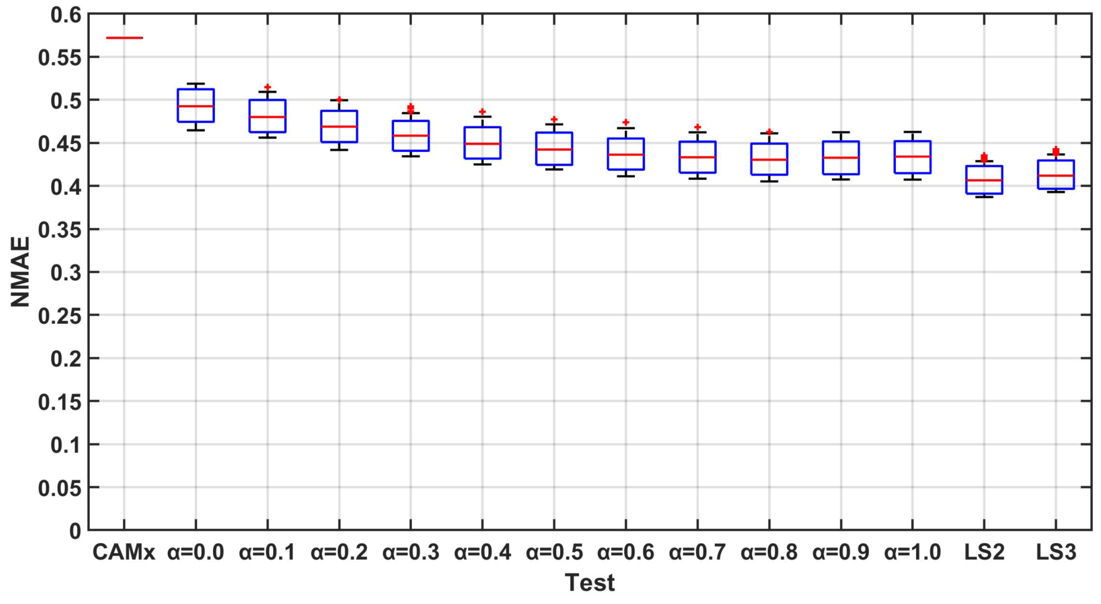
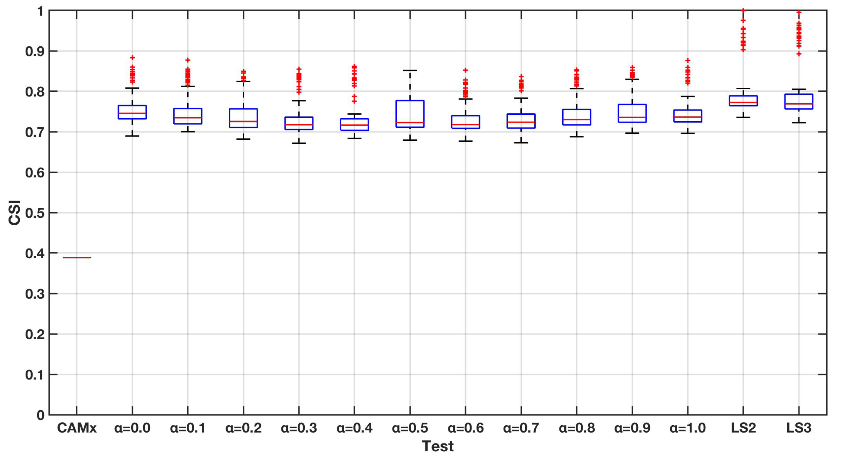
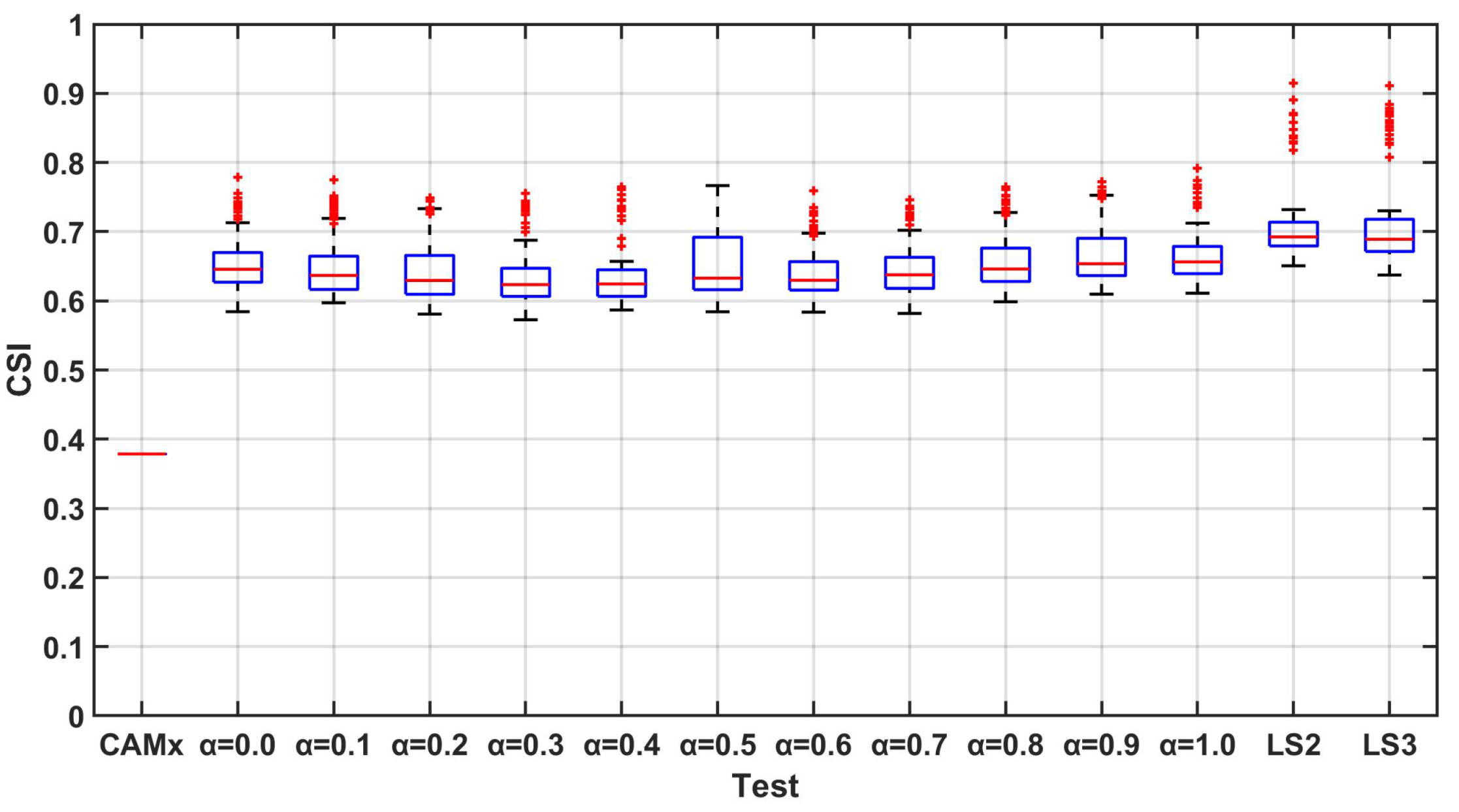
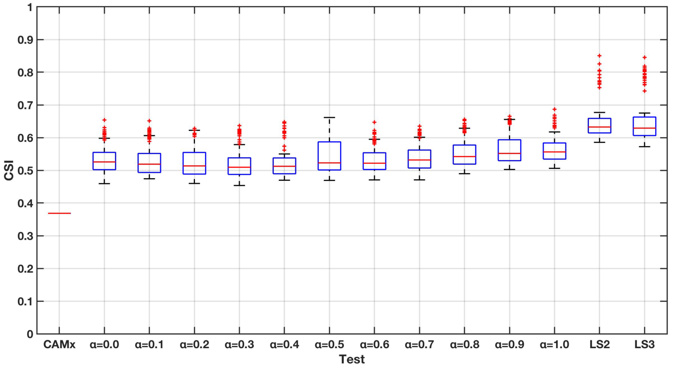
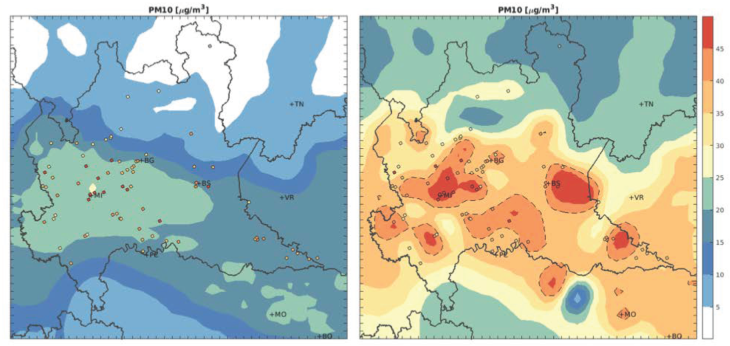
3. Case Study
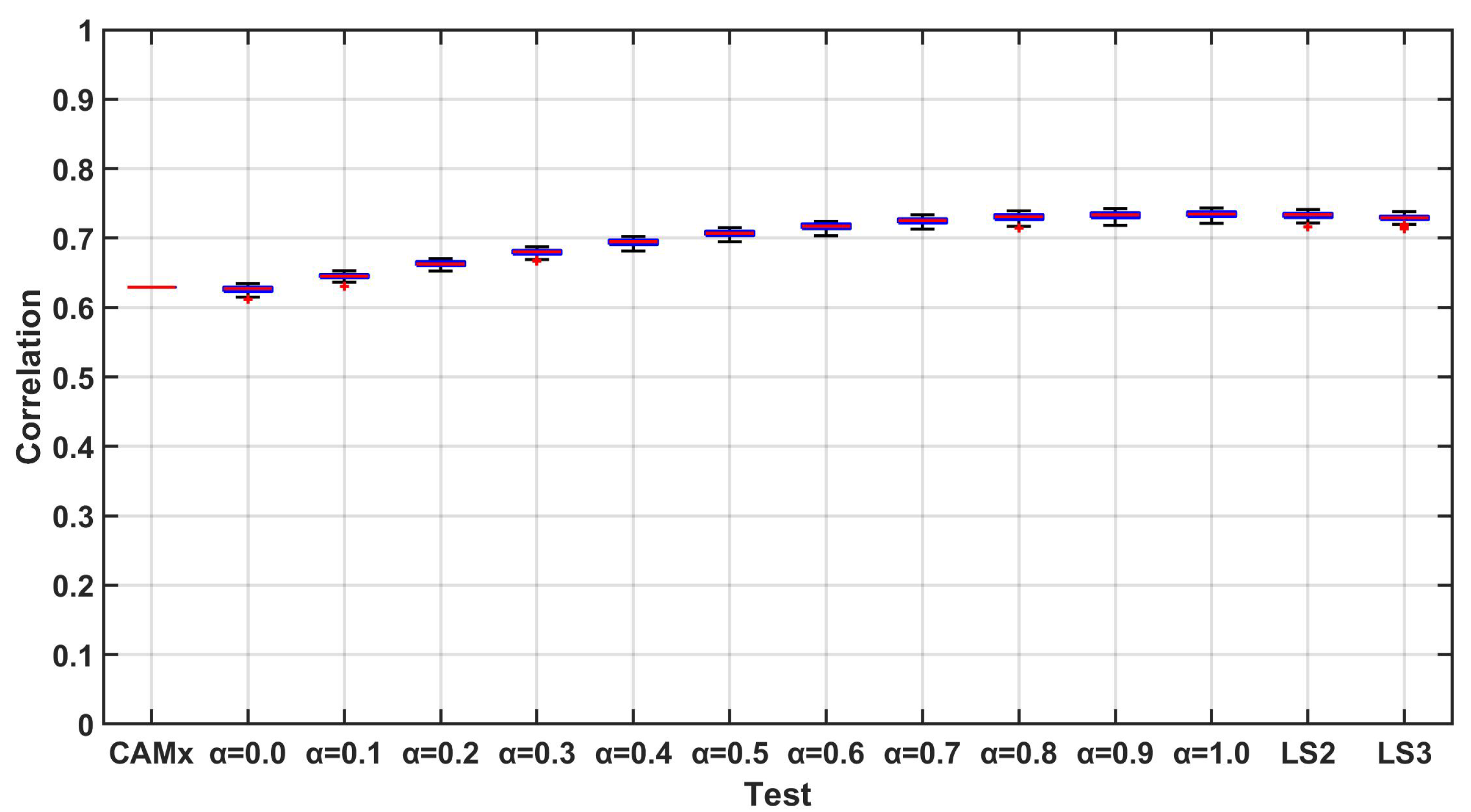
- a test (CAMx) with only measurement data used to correct the initial condition of the forecast;
- 11 tests computed applying the methods in Section 2.1.3 with ranging from 0 to 1 with a step of 0.1;
- two tests with integration performed following the least-square error approach (Section 2.1.4) with m = 2 () and m = 3 ().
4. Conclusions
Author Contributions
Funding
Conflicts of Interest
Abbreviations
| CAMx | Comprehensive Air quality Model with extension |
| CMAQ | Community Multiscale Air Quality model |
| CO | Carbon monoxide |
| CORINAIR | Core inventory air emissions |
| CTM | Chemical Transport Model |
| DSS | Decision Support System |
| EMEP | European Monitoring and Evaluation Programme |
| EMIMO | Emission Model |
| FFNs | Feedforward Neural Networks |
| LOTOS-EUROS | Long Term Ozone Simulation-European Operational Smog |
| MACC | Monitoring Atmospheric Composition and Climate |
| MM5 | Fifth-Generation Mesoscale Model |
| NH3 | Ammonia |
| NOx | Nitrogen oxides |
| PM | Particulate Matter |
| PM10 | Particulate Matter with diameter lower than 10 |
| PREV’AIR | Previsions et Observations de la Qualite de l’Air en France et en Europe |
| PROPART | Dutch PM forecast statistical model |
| SO2 | Sulphur dioxide |
| WRF | Weather Research and Forecasting model |
| PM10 Estimated re-analyzed field forecasted at time t (output of the system) | |
| PM10 computed re-analyzed field at time t (computed on the basis of measurement) | |
| PM10 measurements vector at time t | |
| PM10 background field at time t (output of CAMx model) | |
| VOC | Volatile Organic Compounds |
| Correction computed on the basis of the available measurement at time t | |
| Correction estimated at time t |
References
- Landrigan, P.J.; Fuller, R.; Acosta, N.J.R.; Adeyi, O.; Arnold, R.; Basu, N.N.; Baldé, A.B.; Bertollini, R.; Bose-O’Reilly, S.; Boufford, J.I.; et al. The Lancet Commission on pollution and health. Lancet 2018, 391, 462–512. [Google Scholar] [CrossRef] [Green Version]
- Pope, C.; Dockery, D. Acute health effects of PM10 pollution on symptomatic and non-symptomatic children. Am. Rev. Respir. Dis. 1992, 145, 1123–1128. [Google Scholar] [CrossRef]
- Pope, C.; Dockery, D.; Spengler, J.; Raizenne, M. Respiratory health and PM10 pollution. A daily time series analysis. Am. Rev. Respir. Dis. 1991, 144, 668–674. [Google Scholar] [CrossRef]
- Blond, N.; Carnevale, C.; Douros, J.; Finzi, G.; Guariso, G.; Janssen, S.; Maffeis, G.; Martilli, A.; Pisoni, E.; Real, E.; et al. A framework for integrated assessment modelling. In SpringerBriefs in Applied Sciences and Technology; Springer: Berlin, Germany, 2017; pp. 9–35. [Google Scholar]
- Turrini, E.; Carnevale, C.; Finzi, G.; Volta, M. A non-linear optimization programming model for air quality planning including co-benefits for GHG emissions. Sci. Total Environ. 2018, 621, 980–989. [Google Scholar] [CrossRef]
- Relvas, H.; Miranda, A.; Carnevale, C.; Maffeis, G.; Turrini, E.; Volta, M. Optimal air quality policies and health: A multi-objective nonlinear approach. Environ. Sci. Pollut. Res. 2017, 24, 13687–13699. [Google Scholar] [CrossRef]
- Carnevale, C.; Finzi, G.; Pederzoli, A.; Turrini, E.; Volta, M.; Ferrari, F.; Gianfreda, R.; Maffeis, G. Impact of pollutant emission reductions on summertime aerosol feedbacks: A case study over the PO valley. Atmos. Environ. 2015, 122, 41–57. [Google Scholar] [CrossRef]
- Turrini, E.; Vlachokostas, C.; Volta, M. Combining a Multi-Objective Approach and Multi-Criteria Decision Analysis to Include the Socio-Economic Dimension in an Air Quality Management Problem. Atmosphere 2019, 10, 381. [Google Scholar] [CrossRef] [Green Version]
- Seinfeld, J.H.; Pandis, S.N. Atmospheric Chemistry and Physics; John Wiley & Sons: Hoboken, NJ, USA, 1997. [Google Scholar]
- Carnevale, C.; Finzi, G.; Pisoni, E.; Volta, M. Lazy Learning based surrogate models for air quality planning. Environ. Model. Softw. 2016, 83, 47–57. [Google Scholar] [CrossRef]
- Stadlober, E.; Hörmann, S.; Pfeiler, B. Quality and performance of a PM10 daily forecasting model. Atmos. Environ. 2008, 42, 1098–1109. [Google Scholar] [CrossRef]
- Corani, G. Air quality prediction in Milan: Feed-forward neural networks, pruned neural networks and lazy learning. Ecol. Model. 2005, 185, 513–529. [Google Scholar] [CrossRef] [Green Version]
- Carnevale, C.; Finzi, G.; Pisoni, E.; Singh, V.; Volta, M. An integrated air quality forecast system for a metropolitan area. J. Environ. Monit. 2011, 13, 3437–3447. [Google Scholar] [CrossRef]
- Grivas, G.; Chaloulakou, A. Artificial neural network models for prediction of PM10 hourly concentrations, in the Greater Area of Athens, Greece. Atmos. Environ. 2006, 40, 1216–1229. [Google Scholar] [CrossRef]
- Carnevale, C.; Finzi, G.; Pederzoli, A.; Pisoni, E.; Thunis, P.; Turrini, E.; Volta, M. Applying the delta tool to support the Air Quality Directive: Evaluation of the TCAM chemical transport model. Air Qual. Atmos. Health 2014, 7, 335–346. [Google Scholar] [CrossRef]
- José, R.S.; Pérez, J.L.; Morant, J.L.; González, R.M. European operational air quality forecasting system by using MM5–CMAQ–EMIMO tool. Simul. Model. Pract. Theory 2008, 16, 1534–1540. [Google Scholar] [CrossRef]
- Honoré, C.; Menut, L.; Bessagnet, B.; Meleux, F.; Rouïl, L.; Vautard, R.; Poisson, N.; Peuch, V. PREV’AIR: A Platform for Air Quality Monitoring and Forecasting; Development in Environmental Science, Elsevier: Amsterdam, The Netherlands, 2007; Volume 6, pp. 292–300. [Google Scholar]
- Manders, A.; Schaap, M.; Hoogerbrugge, R. Testing the capability of the chemistry transport model LOTOS-EUROS to forecast PM10 levels in the Netherlands. Atmos. Environ. 2009, 43, 4050–4059. [Google Scholar] [CrossRef]
- Marécal, V.; Peuch, V.H.; Andersson, C.; Andersson, S.; Arteta, J.; Beekmann, M.; Benedictow, A.; Bergström, R.; Bessagnet, B.; Cansado, A.; et al. A regional air quality forecasting system over Europe: The MACC-II daily ensemble production. Geosci. Model. Dev. 2015, 8, 2777–2813. [Google Scholar] [CrossRef] [Green Version]
- Ghil, M.; Malanotte-Rizzoli, P. Data Assimilation in Meteorology and Oceanography. Adv. Geophys. 1991, 33, 141–266. [Google Scholar]
- Bocquet, M.; Elbern, H.; Eskes, H.; Hirtl, M.; Žabkar, R.; Carmichael, G.R.; Flemming, J.; Inness, A.; Pagowski, M.; Camaño, J.L.P.; et al. Data assimilation in atmospheric chemistry models: Current status and future prospects for coupled chemistry meteorology models. Atmos. Chem. Phys. 2015, 15, 5325–5358. [Google Scholar] [CrossRef] [Green Version]
- Denby, B.; Schaap, M.; Segers, A.; Builtjes, P.; Horálek, J. Comparison of two data assimilation methods for assessing PM10 exceedances on the European scale. Atmos. Environ. 2008, 42, 7122–7134. [Google Scholar] [CrossRef]
- Blond, N.; Bel, L.; Vautard, R. Three-dimensional ozone data analysis with an air quality model over the Paris area. J. Geophys. Res. Atmos. 2003, 108, 4744. [Google Scholar] [CrossRef]
- Van de Kassteele, J.; Koelemeijer, R.; Dekkers, A.; Schaap, M.; Homan, C.; Stein, A. Statistical mapping of PM10 concentrations over Western Europe using secondary information from dispersion modeling and MODIS satellite observations. Stoch. Environ. Res. Risk Assess. 2006, 21, 183–194. [Google Scholar] [CrossRef]
- Horálek, J.; Denby, B.; de Smet, P.; de Leeuw, F.; Kurfürst, P.; Swart, R.; van Noije, T. Spatial Mapping of Air Quality for European Scale Assessment; ETC/ACC: Copenhagen, Denmark, 2006. [Google Scholar]
- Curier, R.; Timmermans, R.; Calabretta-Jongen, S.; Eskes, H.; Segers, A.; Swart, D.; Schaap, M. Improving ozone forecasts over Europe by synergistic use of the LOTOS-EUROS chemical transport model and in-situ measurements. Atmos. Environ. 2012, 60, 217–226. [Google Scholar] [CrossRef]
- Neal, L.; Agnew, P.; Moseley, S.; Ordonez, C.; Savage, N.; Tilbee, M. Application of a statistical post-processing technique to a gridded, operational, air quality forecast. Atmos. Environ. 2014, 98, 385–393. [Google Scholar] [CrossRef]
- Eibern, H.; Schmidt, H. A four-dimensional variational chemistry data assimilation scheme for Eulerian chemistry transport modeling. J. Geophys. Res. Atmos. 1999, 104, 18583–18598. [Google Scholar] [CrossRef]
- Van Loon, M.; Builtjes, P.J.; Segers, A. Data assimilation of ozone in the atmospheric transport chemistry model LOTOS. Environ. Model. Softw. 2000, 15, 603–609. [Google Scholar] [CrossRef]
- Constantinescu, E.M.; Sandu, A.; Chai, T.; Carmichael, G.R. Assessment of ensemble-based chemical data assimilation in an idealized setting. Atmos. Environ. 2007, 41, 18–36. [Google Scholar] [CrossRef]
- Environ. CAMx User’s Guide Version 6.50. Available online: http://www.camx.com/files/camxusersguide_v6-50.pdf (accessed on 8 January 2020).
- Carnevale, C.; De Angelis, E.; Finzi, G.; Pederzoli, A.; Turrini, E.; Volta, M. A non linear model approach to define priority for air quality control. IFAC-PapersOnLine 2018, 51, 210–215. [Google Scholar] [CrossRef]
- Carnevale, C.; De Angelis, E.; Finzi, G.; Turrini, E.; Volta, M. An integrated forecasting system for air quality control. In Proceedings of the 2019 18th European Control Conference, ECC 2019, Budapest, Hungary, 23–26 August 2019; pp. 830–835. [Google Scholar]
- Skamarock, W.; Klemp, J.; Dudhia, J.; Gill, D.; Barker, D.; Duda, M.; Huang, X.; Wang, W.; Powers, J. A Description of the Advanced Research WRF Version 3: NCAR/TN-475; National Center for Atmospheric Research: Boulder, CO, USA, 2008; Volume 88. [Google Scholar]
- Evensen, G. Inverse methods and data assimilation in nonlinear ocean models. Phys. D Nonlinear Phenom. 1994, 77, 108–129. [Google Scholar] [CrossRef]
- Carnevale, C.; Finzi, G.; Pederzoli, A.; Pisoni, E.; Thunis, P.; Turrini, E.; Volta, M. A methodology for the evaluation of re-analyzed PM 10 concentration fields: A case study over the PO Valley. Air Qual. Atmos. Health 2015, 8, 533–544. [Google Scholar] [CrossRef]
- Candiani, G.; Carnevale, C.; Finzi, G.; Pisoni, E.; Volta, M. A comparison of reanalysis techniques: Applying optimal interpolation and Ensemble Kalman Filtering to improve air quality monitoring at mesoscale. Sci. Total Environ. 2013, 458–460, 7–14. [Google Scholar] [CrossRef]
- Vestreng, V.; Adams, M.; Goodwin, J. Inventory Review 2004. Emission Data Reportedd to CRLTAP and under the NEC Directive; EMEP/EEA: Copenhagen, Denmark, 2004. [Google Scholar]


| CORINAIR Macrosector | VOC | NH3 | NOx | PM10 | PM2.5 | SO2 |
|---|---|---|---|---|---|---|
| Combustion in energy and transformation industries | 3015 | 59 | 33,595 | 942 | 826 | 9641 |
| Non-industrial combustion plants | 73,197 | 1090 | 46,267 | 44,064 | 43,248 | 622 |
| Combustion in manufacturing industry | 8233 | 778 | 72,022 | 4934 | 3435 | 29730 |
| Production processes | 40,056 | 1212 | 12,950 | 4425 | 2408 | 16,440 |
| Fossil fuel and geothermal energy distribution | 28,187 | 0 | 358 | 82 | 74 | 1257 |
| Solvent and other product use | 232,831 | 103 | 680 | 1072 | 853 | 13 |
| Road transport | 68,706 | 4831 | 260,829 | 21,930 | 16,479 | 644 |
| Other mobile sources and machinery | 15,329 | 15 | 65,095 | 6297 | 5004 | 4446 |
| Waste treatment and disposal | 3376 | 2708 | 6348 | 1153 | 1057 | 1185 |
| Agriculture | 153,400 | 304,835 | 6513 | 7521 | 2957 | 222 |
| Biogenic | 205,606 | 42 | 12,798 | 10,142 | 6173 | 234 |
| TOTAL | 831,936 | 315,673 | 517,455 | 102,562 | 82,514 | 64,434 |
| Forecasted | Observed | Total | |
|---|---|---|---|
| Yes | No | ||
| Yes | Hits (YY) | False Alarm (YN) | YY+YN |
| No | Missess (NY) | Correctly Rejected (NN) | NY+NN |
| Total | YY+NY | YN+NN | YY+YN+NY+NN |
© 2020 by the authors. Licensee MDPI, Basel, Switzerland. This article is an open access article distributed under the terms and conditions of the Creative Commons Attribution (CC BY) license (http://creativecommons.org/licenses/by/4.0/).
Share and Cite
Carnevale, C.; Angelis, E.D.; Finzi, G.; Turrini, E.; Volta, M. Application of Data Fusion Techniques to Improve Air Quality Forecast: A Case Study in the Northern Italy. Atmosphere 2020, 11, 244. https://0-doi-org.brum.beds.ac.uk/10.3390/atmos11030244
Carnevale C, Angelis ED, Finzi G, Turrini E, Volta M. Application of Data Fusion Techniques to Improve Air Quality Forecast: A Case Study in the Northern Italy. Atmosphere. 2020; 11(3):244. https://0-doi-org.brum.beds.ac.uk/10.3390/atmos11030244
Chicago/Turabian StyleCarnevale, Claudio, Elena De Angelis, Giovanna Finzi, Enrico Turrini, and Marialuisa Volta. 2020. "Application of Data Fusion Techniques to Improve Air Quality Forecast: A Case Study in the Northern Italy" Atmosphere 11, no. 3: 244. https://0-doi-org.brum.beds.ac.uk/10.3390/atmos11030244