Evaluation of the Soil, Vegetation, and Snow (SVS) Land Surface Model for the Simulation of Surface Energy Fluxes and Soil Moisture under Snow-Free Conditions

 , , ,
, , ,
Abstract
:1. Introduction
2. Methodology
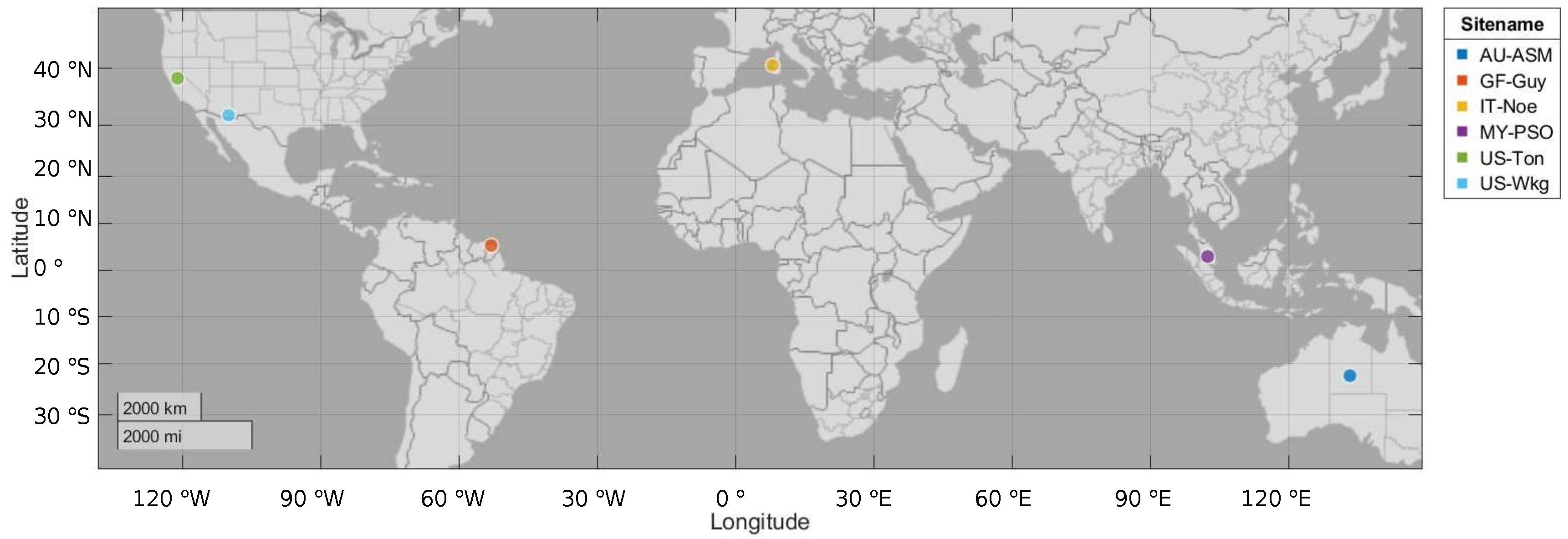
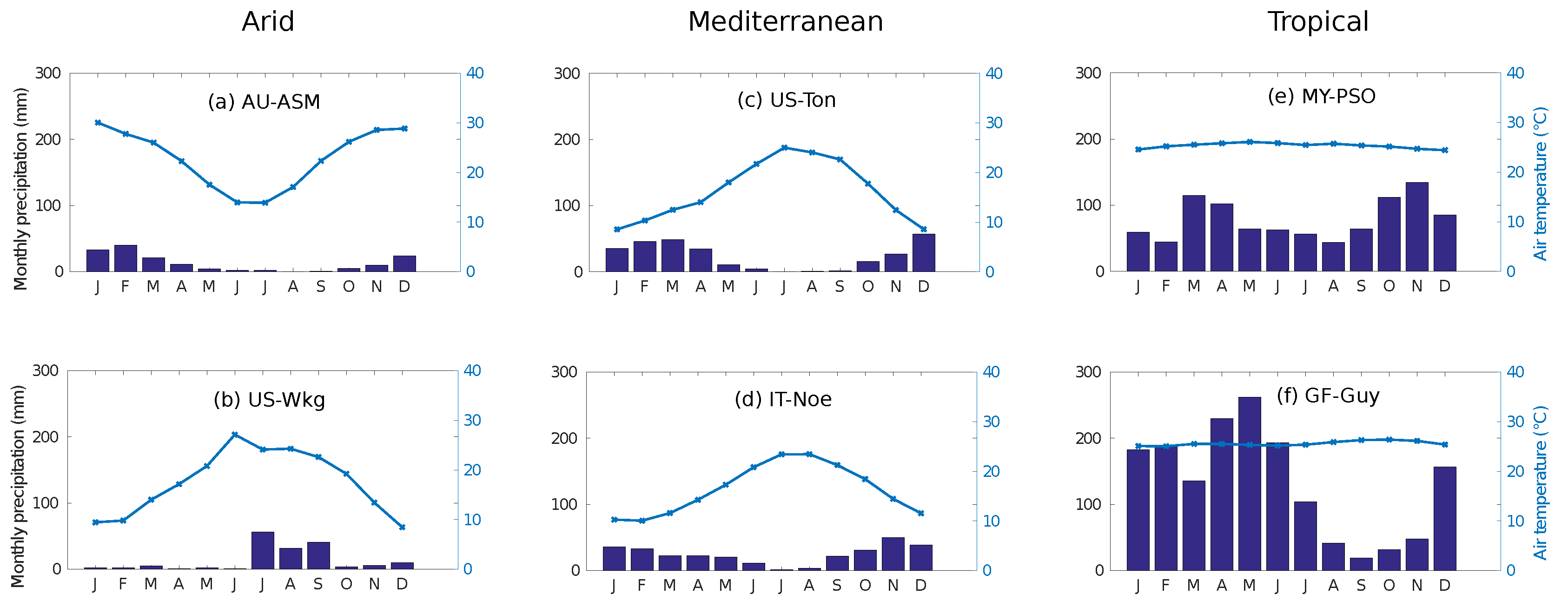
2.1. Study Sites
2.2. Data
2.3. Land Surface Models
2.3.1. SVS
2.3.2. CLASS
2.3.3. Differences between SVS and CLASS
2.4. Experimental Setup
2.5. Modeling Performance
3. Result and Discussion
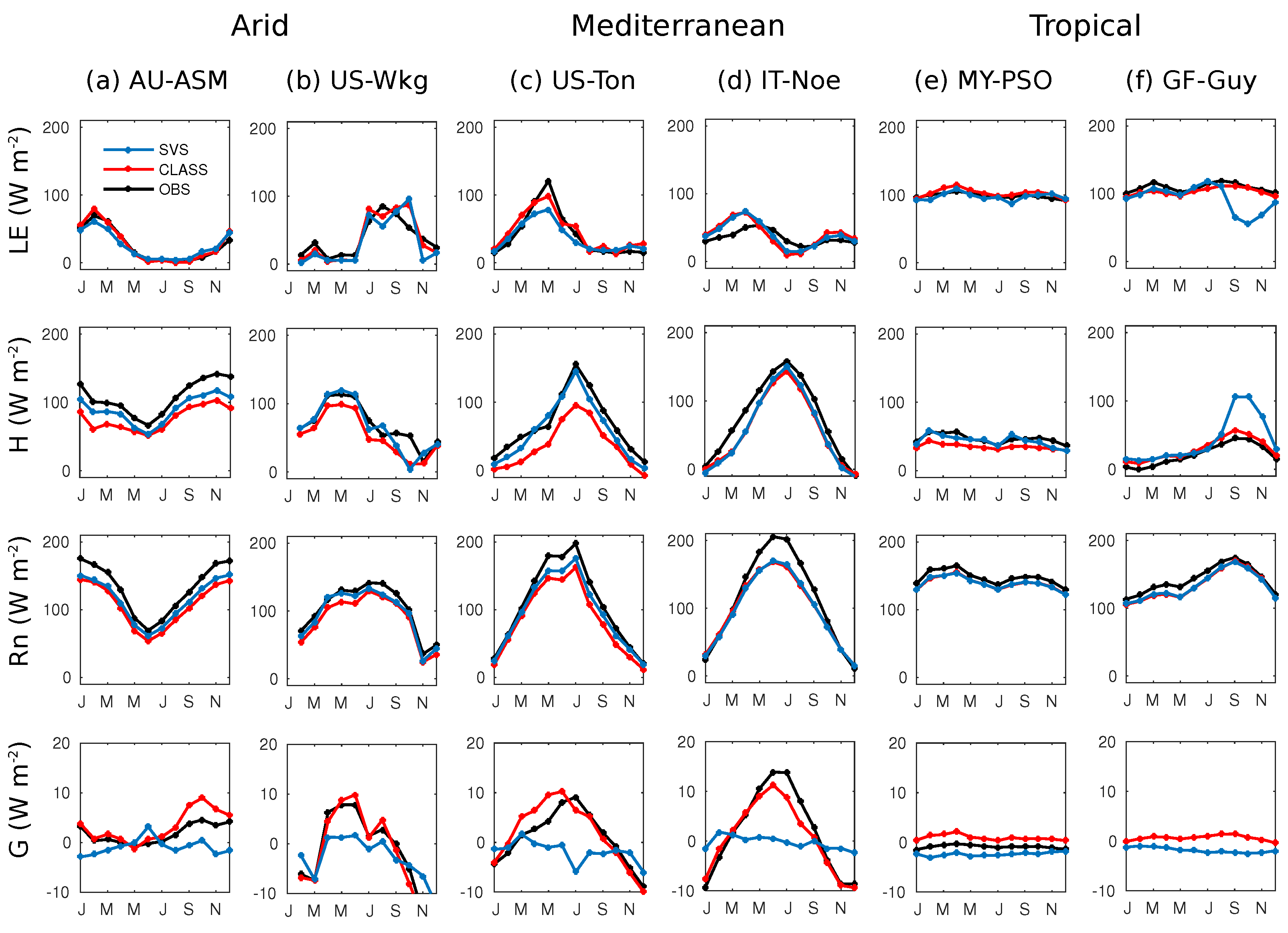
3.1. Energy Fluxes
3.1.1. Arid Sites
3.1.2. Mediterranean Sites
3.1.3. Tropical Sites
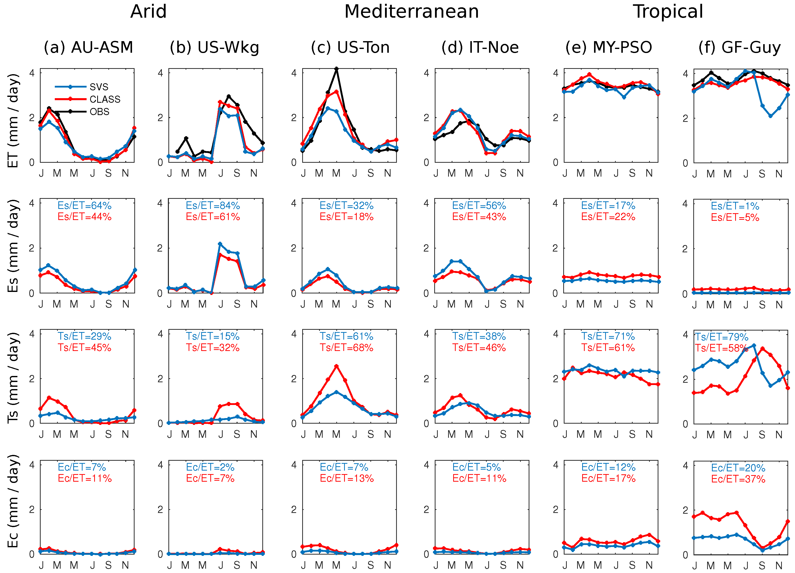
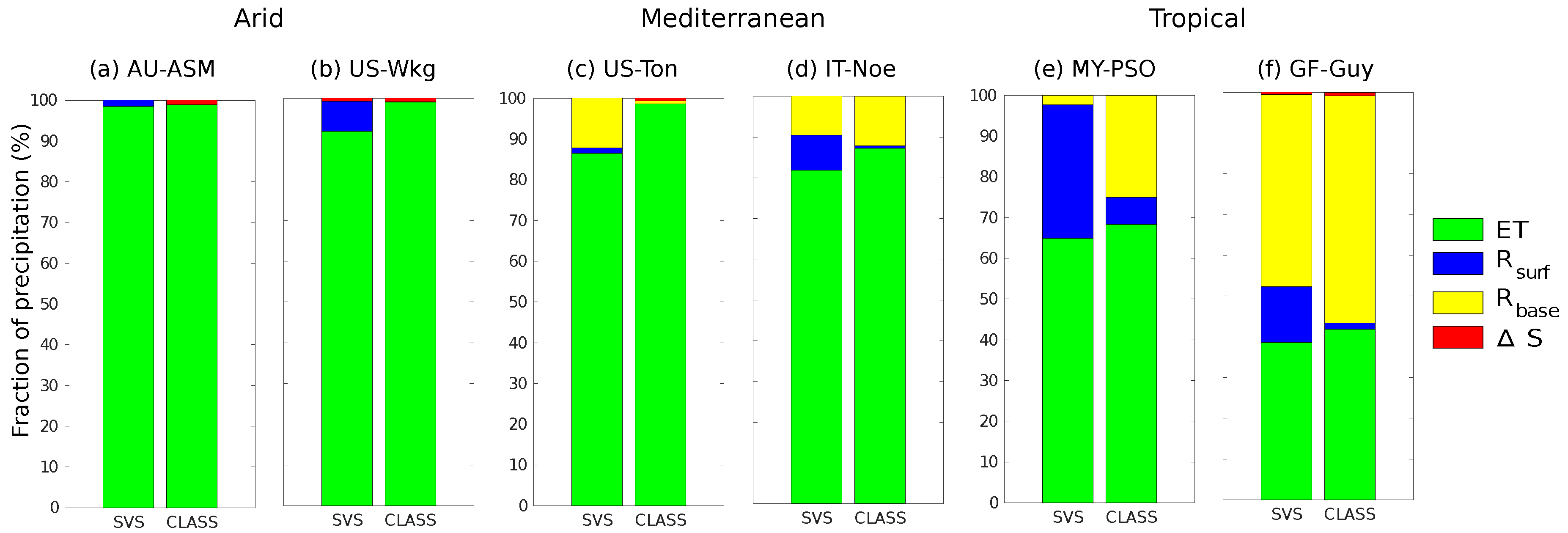
3.2. Partitioning of Evapotranspiration
3.3. Sources of Uncertainties Associated with Energy Fluxes
3.4. Water Balance
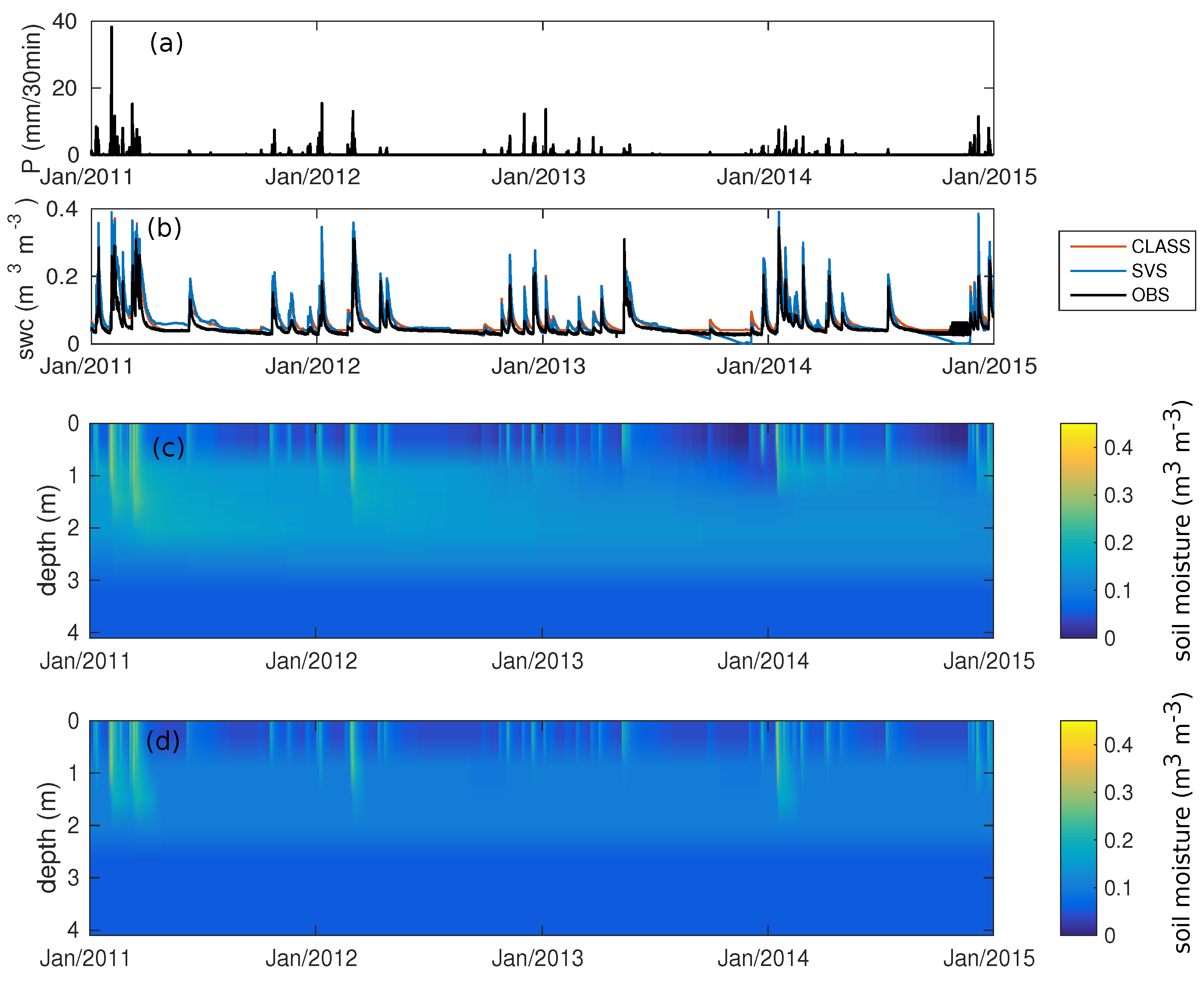
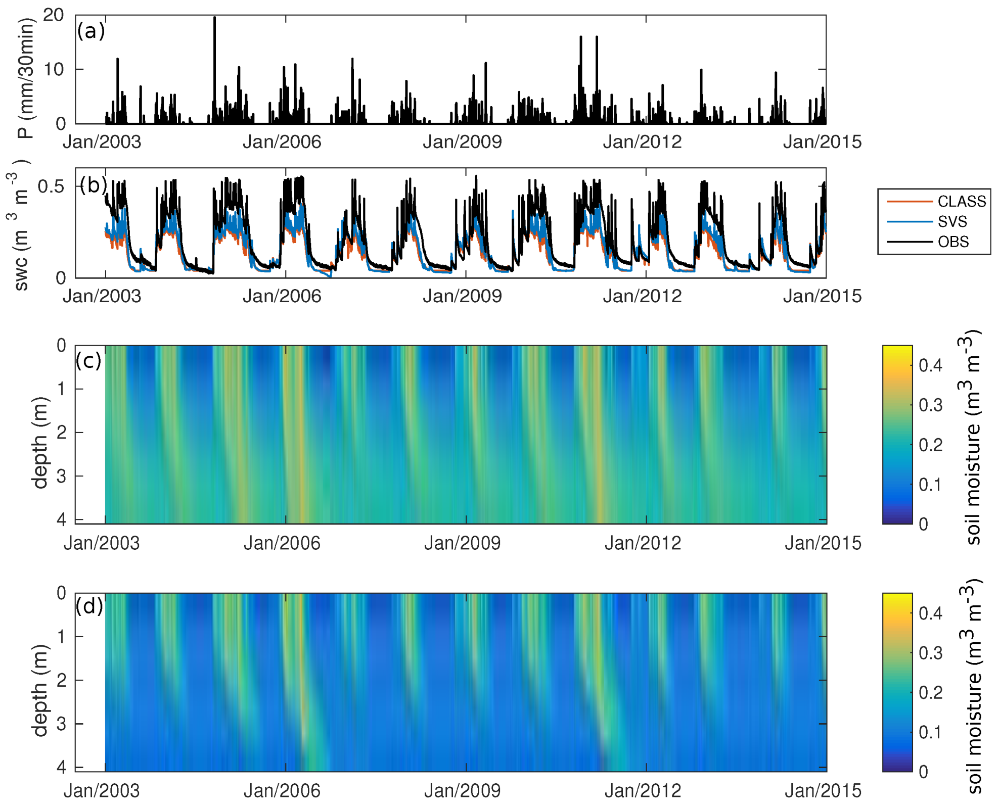
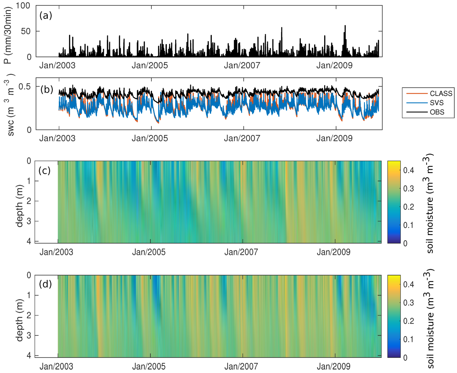
3.5. Soil Moisture
3.5.1. Arid Sites
3.5.2. Mediterranean Sites
3.5.3. Tropical
3.6. Uncertainties Associated with Soil Moisture
4. Conclusions
- The albedo of vegetation is simply based on a weighted mean of look-up table values of fixed albedos. This scheme may lead to a negative bias of up to 12% in the net shortwave radiation and 13% in the net radiation. Albedo is specified the same way as root depth, density and LAI. These are all parameters that can be improved and will impact SVS simulations. The photosynthesis also has several look up tables for various key parameters controlling the stomatal resistance. External databases and satellite-derived approximation could help better specify some of these parameters.
- Abrupt underestimations of at GF-Guy site is mainly associated with transpiration simulations. Thus, further attention should be given to this process.
- Poorly simulated G is associated with the simple method used (residual of the other energy fluxes) and the single-layer description of the soil. To avoid these structural biases, vertical transport of heat in the soil along with multilayer-energy balance would be an asset in the soil description.
- The better simulation of soil moisture with CLASS in arid sites suggests that certain features, such as the inclusion of residual saturation when defining water retention curves, can be advantageous. Alternatively, limits on evaporation and moisture stress parameterizations may help to prevent soil moisture to reach zero values.
- Surface soil moisture at tropical sites should take into account organic matter.
Author Contributions
Funding
Acknowledgments
Conflicts of Interest
References
- Dirmeyer, P.A. Using a global soil wetness dataset to improve seasonal climate simulation. J. Clim. 2000, 13, 2900–2922. [Google Scholar] [CrossRef]
- Koster, R.D.; Suarez, M.J.; Ducharne, A.; Stieglitz, M.; Kumar, P. A catchment-based approach to modeling land surface processes in a general circulation model: 1. Model structure. J. Geophys. Res. Atmos. 2000, 105, 24809–24822. [Google Scholar] [CrossRef]
- Rodell, M.; Houser, P.R.; Jambor, U.; Gottschalck, J.; Mitchell, K.; Meng, C.J.; Arsenault, K.; Cosgrove, B.; Radakovich, J.; Bosilovich, M.; et al. The global land data assimilation system. Bull. Am. Meteorol. Soc. 2004, 85, 381–394. [Google Scholar] [CrossRef] [Green Version]
- Mitchell, K.E.; Lohmann, D.; Houser, P.R.; Wood, E.F.; Schaake, J.C.; Robock, A.; Cosgrove, B.A.; Sheffield, J.; Duan, Q.; Luo, L.; et al. The multi-institution North American Land Data Assimilation System (NLDAS): Utilizing multiple GCIP products and partners in a continental distributed hydrological modeling system. J. Geophys. Res. Atmos. 2004, 109. [Google Scholar] [CrossRef] [Green Version]
- Carrera, M.L.; Bélair, S.; Fortin, V.; Bilodeau, B.; Charpentier, D.; Doré, I. Evaluation of snowpack simulations over the Canadian Rockies with an experimental hydrometeorological modeling system. J. Hydrometeorol. 2010, 11, 1123–1140. [Google Scholar] [CrossRef]
- Gaborit, É.; Fortin, V.; Xu, X.; Seglenieks, F.; Tolson, B.; Fry, L.M.; Hunter, T.; Anctil, F.; Gronewold, A.D. A Hydrological Prediction System Based on the SVS Land-Surface Scheme: Efficient calibration of GEM-Hydro for streamflow simulation over the Lake Ontario basin. Hydrol. Earth Syst. Sci. 2017, 21, 4825–4839. [Google Scholar] [CrossRef] [Green Version]
- Pitman, A. The evolution of, and revolution in, land surface schemes designed for climate models. Int. J. Climatol. A J. R. Meteorol. Soc. 2003, 23, 479–510. [Google Scholar] [CrossRef]
- van den Hurk, B.; Best, M.; Dirmeyer, P.; Pitman, A.; Polcher, J.; Santanello, J. Acceleration of land surface model development over a decade of GLASS. Bull. Am. Meteorol. Soc. 2011, 92, 1593–1600. [Google Scholar] [CrossRef] [Green Version]
- Henderson-Sellers, A.; McGuffie, K.; Pitman, A. The project for intercomparison of land-surface parametrization schemes (PILPS): 1992 to 1995. Clim. Dyn. 1996, 12, 849–859. [Google Scholar] [CrossRef]
- Boone, A.; de Rosnay, P.; Balsamo, G.; Beljaars, A.; Chopin, F.; Decharme, B.; Delire, C.; Ducharne, A.; Gascoin, S.; Grippa, M.; et al. The AMMA land surface model intercomparison project (ALMIP). Bull. Am. Meteorol. Soc. 2009, 90, 1865–1880. [Google Scholar] [CrossRef]
- Sueyoshi, T.; Saito, K.; Miyazaki, S.; Mori, J.; Ise, T.; Arakida, H.; Suzuki, R.; Sato, A.; Iijima, Y.; Yabuki, H.; et al. The GRENE-TEA Model Intercomparison Project (GTMIP) stage 1 forcing dataset. Earth Syst. Sci. Data 2015, 8, 703–736. [Google Scholar] [CrossRef]
- Blyth, E.; Gash, J.; Lloyd, A.; Pryor, M.; Weedon, G.P.; Shuttleworth, J. Evaluating the JULES land surface model energy fluxes using FLUXNET data. J. Hydrometeorol. 2010, 11, 509–519. [Google Scholar] [CrossRef] [Green Version]
- Stöckli, R.; Vidale, P.L. Modeling diurnal to seasonal water and heat exchanges at European Fluxnet sites. Theor. Appl. Climatol. 2005, 80, 229–243. [Google Scholar] [CrossRef]
- Verseghy, D.L. CLASS—A Canadian land surface scheme for GCMs. I. Soil model. Int. J. Climatol. 1991, 11, 111–133. [Google Scholar] [CrossRef]
- Verseghy, D.L.; McFarlane, N.; Lazare, M. CLASS—A Canadian land surface scheme for GCMs, II. Vegetation model and coupled runs. Int. J. Climatol. 1993, 13, 347–370. [Google Scholar] [CrossRef]
- Schlosser, C.A.; Slater, A.G.; Robock, A.; Pitman, A.J.; Vinnikov, K.Y.; Henderson-Sellers, A.; Speranskaya, N.A.; Mitchell, K. Simulations of a boreal grassland hydrology at Valdai, Russia: PILPS Phase 2 (d). Mon. Weather Rev. 2000, 128, 301–321. [Google Scholar] [CrossRef]
- Slater, A.G.; Schlosser, C.A.; Desborough, C.E.; Pitman, A.J.; Henderson-Sellers, A.; Robock, A.; Vinnikov, K.Y.; Entin, J.; Mitchell, K.; Chen, F.; et al. The representation of snow in land surface schemes: Results from PILPS 2 (d). J. Hydrometeorol. 2001, 2, 7–25. [Google Scholar] [CrossRef] [Green Version]
- Bowling, L.C.; Lettenmaier, D.P.; Nijssen, B.; Graham, L.; Clark, D.B.; Maayar, M.E.; Essery, R.; Goers, S.; Gusev, Y.M.; Habets, F.; et al. Simulation of high-latitude hydrological processes in the Torne–Kalix basin: PILPS Phase 2 (e): 1: Experiment description and summary intercomparisons. Glob. Planet. Chang. 2003, 38, 1–30. [Google Scholar] [CrossRef] [Green Version]
- Rutter, N.; Essery, R.; Pomeroy, J.; Altimir, N.; Andreadis, K.; Baker, I.; Barr, A.; Bartlett, P.; Boone, A.; Deng, H.; et al. Evaluation of forest snow processes models (SnowMIP2). J. Geophys. Res. Atmos. 2009, 114. [Google Scholar] [CrossRef] [Green Version]
- Bartlett, P.A.; McCaughey, J.H.; Lafleur, P.M.; Verseghy, D.L. Performance of the Canadian land surface scheme at temperate aspen-birch and mixed forests, and a boreal young jack pine forest: Tests involving canopy conductance parametrizations. Atmos. Ocean 2000, 38, 113–140. [Google Scholar] [CrossRef] [Green Version]
- Bartlett, P.A.; Harry McCaughey, J.; Lafleur, P.M.; Verseghy, D.L. Modelling evapotranspiration at three boreal forest stands using the CLASS: Tests of parameterizations for canopy conductance and soil evaporation. Int. J. Climatol. A J. R. Meteorol. Soc. 2003, 23, 427–451. [Google Scholar] [CrossRef] [Green Version]
- Wang, S.; Grant, R.; Verseghy, D.; Black, T. Modelling plant carbon and nitrogen dynamics of a boreal aspen forest in CLASS—the Canadian Land Surface Scheme. Ecol. Model. 2001, 142, 135–154. [Google Scholar] [CrossRef]
- Arain, M.; Black, T.; Barr, A.; Jarvis, P.; Massheder, J.; Verseghy, D.; Nesic, Z. Effects of seasonal and interannual climate variability on net ecosystem productivity of boreal deciduous and conifer forests. Can. J. For. Res. 2002, 32, 878–891. [Google Scholar] [CrossRef]
- Verseghy, D.; Brown, R.; Wang, L. Evaluation of CLASS snow simulation over eastern Canada. J. Hydrometeorol. 2017, 18, 1205–1225. [Google Scholar] [CrossRef]
- Isabelle, P.E.; Nadeau, D.F.; Asselin, M.H.; Harvey, R.; Musselman, K.N.; Rousseau, A.N.; Anctil, F. Solar radiation transmittance of a boreal balsam fir canopy: Spatiotemporal variability and impacts on growing season hydrology. Agric. For. Meteorol. 2018, 263, 1–14. [Google Scholar] [CrossRef]
- Comer, N.T.; Lafleur, P.M.; Roulet, N.T.; Letts, M.G.; Skarupa, M.; Verseghy, D. A test of the Canadian Land Surface Scheme (CLASS) for a variety of wetland types. Atmos. Ocean 2000, 38, 161–179. [Google Scholar] [CrossRef]
- Lafleur, P.M.; Skarupa, M.R.; Verseghy, D.L. Validation of the Canadian Land Surface Scheme (CLASS) for a subarctic open woodland. Atmos. Ocean 2000, 38, 205–225. [Google Scholar] [CrossRef]
- Brown, R.; Bartlett, P.; MacKay, M.; Verseghy, D. Evaluation of snow cover in CLASS for SnowMIP. Atmos. Ocean 2006, 44, 223–238. [Google Scholar] [CrossRef]
- Wen, L.; Wu, Z.; Lu, G.; Lin, C.A.; Zhang, J.; Yang, Y. Analysis and improvement of runoff generation in the land surface scheme CLASS and comparison with field measurements from China. J. Hydrol. 2007, 345, 1–15. [Google Scholar] [CrossRef]
- Alves, M.; Music, B.; Nadeau, D.F.; Anctil, F. Comparing the Performance of the Maximum Entropy Production Model With a Land Surface Scheme in Simulating Surface Energy Fluxes. J. Geophys. Res. Atmos. 2019, 124, 3279–3300. [Google Scholar] [CrossRef]
- Pietroniro, A.; Fortin, V.; Kouwen, N.; Neal, C.; Turcotte, R.; Davison, B.; Verseghy, D.; Soulis, E.D.; Caldwell, R.; Evora, N.; et al. Development of the MESH modelling system for hydrological ensemble forecasting of the Laurentian Great Lakes at the regional scale. Hydrol. Earth Syst. Sci. 2007, 11, 1279–1294. [Google Scholar] [CrossRef] [Green Version]
- Haghnegahdar, A.; Tolson, B.A.; Craig, J.R.; Paya, K.T. Assessing the performance of a semi-distributed hydrological model under various watershed discretization schemes. Hydrol. Process. 2015, 29, 4018–4031. [Google Scholar] [CrossRef]
- Davison, B.; Fortin, V.; Pietroniro, A.; Yau, M.K.; Leconte, R. Parameter-state ensemble thinning for short-term hydrological prediction. Hydrol. Earth Syst. Sci. 2019, 23, 741–762. [Google Scholar] [CrossRef] [Green Version]
- Abramowitz, G.; Leuning, R.; Clark, M.; Pitman, A. Evaluating the performance of land surface models. J. Clim. 2008, 21, 5468–5481. [Google Scholar] [CrossRef]
- Chen, T.H.; Henderson-Sellers, A.; Milly, P.C.D.; Pitman, A.J.; Beljaars, A.C.M.; Polcher, J.; Abramopoulos, F.; Boone, A.; Chang, S.; Chen, F.; et al. Cabauw experimental results from the project for intercomparison of land-surface parameterization schemes. J. Clim. 1997, 10, 1194–1215. [Google Scholar] [CrossRef] [Green Version]
- Sellers, P.; Dorman, J. Testing the simple biosphere model (SiB) using point micrometeorological and biophysical data. J. Clim. Appl. Meteorol. 1987, 26, 622–651. [Google Scholar] [CrossRef] [Green Version]
- Wang, K.; Dickinson, R.E. A review of global terrestrial evapotranspiration: Observation, modeling, climatology, and climatic variability. Rev. Geophys. 2012, 50. [Google Scholar] [CrossRef]
- Lohmann, D.; Mitchell, K.E.; Houser, P.R.; Wood, E.F.; Schaake, J.C.; Robock, A.; Cosgrove, B.A.; Sheffield, J.; Duan, Q.; Luo, L.; et al. Streamflow and water balance intercomparisons of four land surface models in the North American Land Data Assimilation System project. J. Geophys. Res. Atmos. 2004, 109. [Google Scholar] [CrossRef]
- Lohmann, D.; Lettenmaier, D.P.; Liang, X.; Wood, E.F.; Boone, A.; Chang, S.; Chen, F.; Dai, Y.; Desborough, C.; Dickinson, R.E.; et al. The Project for Intercomparison of Land-surface Parameterization Schemes (PILPS) phase 2(c) Red–Arkansas River basin experiment: 3. Spatial and temporal analysis of water fluxes. Glob. Planet. Chang. 1998, 19, 161–179. [Google Scholar] [CrossRef]
- Bélair, S.; Crevier, L.P.; Mailhot, J.; Bilodeau, B.; Delage, Y. Operational implementation of the ISBA land surface scheme in the Canadian regional weather forecast model. Part I: Warm season results. J. Hydrometeorol. 2003, 4, 352–370. [Google Scholar] [CrossRef]
- Bélair, S.; Brown, R.; Mailhot, J.; Bilodeau, B.; Crevier, L.P. Operational implementation of the ISBA land surface scheme in the Canadian regional weather forecast model. Part II: Cold season results. J. Hydrometeorol. 2003, 4, 371–386. [Google Scholar] [CrossRef]
- Bélair, S.; Roch, M.; Leduc, A.M.; Vaillancourt, P.A.; Laroche, S.; Mailhot, J. Medium-range quantitative precipitation forecasts from Canada’s new 33-km deterministic global operational system. Weather Forecast. 2009, 24, 690–708. [Google Scholar] [CrossRef]
- Alavi, N.; Bélair, S.; Fortin, V.; Zhang, S.; Husain, S.Z.; Carrera, M.L.; Abrahamowicz, M. Warm season evaluation of soil moisture prediction in the Soil, Vegetation, and Snow (SVS) scheme. J. Hydrometeorol. 2016, 17, 2315–2332. [Google Scholar] [CrossRef]
- Husain, S.Z.; Alavi, N.; Bélair, S.; Carrera, M.; Zhang, S.; Fortin, V.; Abrahamowicz, M.; Gauthier, N. The multibudget Soil, Vegetation, and Snow (SVS) scheme for land surface parameterization: Offline warm season evaluation. J. Hydrometeorol. 2016, 17, 2293–2313. [Google Scholar] [CrossRef]
- Vionnet, V.; Fortin, V.; Gaborit, E.; Roy, G.; Abrahamowicz, M.; Gasset, N.; Pomeroy, J.W. High-resolution hydrometeorological modelling of the June 2013 flood in southern Alberta, Canada. Hydrol. Earth Syst. Sci. Discuss. 2019, 2019, 1–36. [Google Scholar] [CrossRef] [Green Version]
- Maheu, A.; Anctil, F.; Gaborit, É.; Fortin, V.; Nadeau, D.F.; Therrien, R. A field evaluation of soil moisture modelling with the Soil, Vegetation, and Snow (SVS) land surface model using evapotranspiration observations as forcing data. J. Hydrol. 2018, 558, 532–545. [Google Scholar] [CrossRef]
- Baldocchi, D.; Falge, E.; Gu, L.; Olson, R.; Hollinger, D.; Running, S.; Anthoni, P.; Bernhofer, C.; Davis, K.; Evans, R.; et al. FLUXNET: A new tool to study the temporal and spatial variability of ecosystem-scale carbon dioxide, water vapor, and energy flux densities. Bull. Am. Meteorol. Soc. 2001, 82, 2415–2434. [Google Scholar] [CrossRef]
- Hutley, L.B.; Beringer, J.; Isaac, P.R.; Hacker, J.M.; Cernusak, L.A. A sub-continental scale living laboratory: Spatial patterns of savanna vegetation over a rainfall gradient in northern Australia. Agric. For. Meteorol. 2011, 151, 1417–1428. [Google Scholar] [CrossRef]
- Adams, D.K.; Comrie, A.C. The north American monsoon. Bull. Am. Meteorol. Soc. 1997, 78, 2197–2214. [Google Scholar] [CrossRef] [Green Version]
- Moran, M.S.; Scott, R.L.; Hamerlynck, E.P.; Green, K.N.; Emmerich, W.E.; Collins, C.D.H. Soil evaporation response to Lehmann lovegrass (Eragrostis lehmanniana) invasion in a semiarid watershed. Agric. For. Meteorol. 2009, 149, 2133–2142. [Google Scholar] [CrossRef]
- Baldocchi, D.; Xu, L.; Kiang, N. How plant functional-type, weather, seasonal drought, and soil physical properties alter water and energy fluxes of an oak–grass savanna and an annual grassland. Agric. For. Meteorol. 2004, 123, 13–39. [Google Scholar] [CrossRef] [Green Version]
- Marras, S.; Pyles, R.D.; Sirca, C.; Snyder, R.; Duce, P.; Spano, D. Evaluation of the Advanced Canopy–Atmosphere–Soil Algorithm (ACASA) model performance over Mediterranean maquis ecosystem. Agric. For. Meteorol. 2011, 151, 730–745. [Google Scholar] [CrossRef]
- Noguchi, S.; Nik, A.R.; Tani, M. Rainfall characteristics of tropical rainforest at Pasoh forest reserve, Negeri Sembilan, Peninsular Malaysia. In Pasoh: Ecology of A Lowland Rain Forest in Southeast Asia; Springer: Berlin, Germany, 2003; pp. 51–58. [Google Scholar]
- Kosugi, Y.; Takanashi, S.; Tani, M.; Ohkubo, S.; Matsuo, N.; Itoh, M.; Noguchi, S.; Nik, A.R. Effect of inter-annual climate variability on evapotranspiration and canopy CO2 exchange of a tropical rainforest in Peninsular Malaysia. J. For. Res. 2012, 17, 227–240. [Google Scholar] [CrossRef]
- Bonal, D.; Bosc, A.; Ponton, S.; Goret, J.Y.; Burban, B.; Gross, P.; Bonnefond, J.M.; Elbers, J.; Longdoz, B.; Epron, D.; et al. Impact of severe dry season on net ecosystem exchange in the Neotropical rainforest of French Guiana. Glob. Chang. Biol. 2008, 14, 1917–1933. [Google Scholar] [CrossRef]
- Gill, A.E. Atmosphere—Ocean Dynamics; Elsevier: Amsterdam, The Netherlands, 2016; pp. 150–155. [Google Scholar]
- Reichstein, M.; Falge, E.; Baldocchi, D.; Papale, D.; Aubinet, M.; Berbigier, P.; Bernhofer, C.; Buchmann, N.; Gilmanov, T.; Granier, A.; et al. On the separation of net ecosystem exchange into assimilation and ecosystem respiration: Review and improved algorithm. Glob. Chang. Biol. 2005, 11, 1424–1439. [Google Scholar] [CrossRef]
- Vuichard, N.; Papale, D. Filling the gaps in meteorological continuous data measured at FLUXNET sites with ERA-Interim reanalysis. Earth Syst. Sci. Data 2015, 7, 157–171. [Google Scholar] [CrossRef] [Green Version]
- Moncrieff, J.B.; Massheder, J.; De Bruin, H.; Elbers, J.; Friborg, T.; Heusinkveld, B.; Kabat, P.; Scott, S.; Søgaard, H.; Verhoef, A. A system to measure surface fluxes of momentum, sensible heat, water vapour and carbon dioxide. J. Hydrol. 1997, 188, 589–611. [Google Scholar] [CrossRef]
- Miller, G.R.; Baldocchi, D.D.; Law, B.E.; Meyers, T. An analysis of soil moisture dynamics using multi-year data from a network of micrometeorological observation sites. Adv. Water Resour. 2007, 30, 1065–1081. [Google Scholar] [CrossRef] [Green Version]
- Keefer, T.O.; Moran, M.S.; Paige, G.B. Long-term meteorological and soil hydrology database, Walnut Gulch Experimental Watershed, Arizona, United States. Water Resour. Res. 2008, 44. [Google Scholar] [CrossRef] [Green Version]
- Cleverly, J.; Boulain, N.; Villalobos-Vega, R.; Grant, N.; Faux, R.; Wood, C.; Cook, P.G.; Yu, Q.; Leigh, A.; Eamus, D. Dynamics of component carbon fluxes in a semi-arid Acacia woodland, central Australia. J. Geophys. Res. Biogeosci. 2013, 118, 1168–1185. [Google Scholar] [CrossRef]
- Farquhar, G.D.; von Caemmerer, S.V.; Berry, J. A biochemical model of photosynthetic CO2 assimilation in leaves of C 3 species. Planta 1980, 149, 78–90. [Google Scholar] [CrossRef] [Green Version]
- Collatz, G.J.; Ball, J.T.; Grivet, C.; Berry, J.A. Physiological and environmental regulation of stomatal conductance, photosynthesis and transpiration: A model that includes a laminar boundary layer. Agric. For. Meteorol. 1991, 54, 107–136. [Google Scholar] [CrossRef]
- Collatz, G.J.; Ribas-Carbo, M.; Berry, J. Coupled photosynthesis-stomatal conductance model for leaves of C4 plants. Funct. Plant Biol. 1992, 19, 519–538. [Google Scholar] [CrossRef]
- Clapp, R.B.; Hornberger, G.M. Empirical equations for some soil hydraulic properties. Water Resour. Res. 1978, 14, 601–604. [Google Scholar] [CrossRef] [Green Version]
- Boone, A.; Calvet, J.C.; Noilhan, J. Inclusion of a third soil layer in a land surface scheme using the force–restore method. J. Appl. Meteorol. 1999, 38, 1611–1630. [Google Scholar] [CrossRef]
- Soulis, E.; Craig, J.; Fortin, V.; Liu, G. A simple expression for the bulk field capacity of a sloping soil horizon. Hydrol. Process. 2011, 25, 112–116. [Google Scholar] [CrossRef]
- Brooks, R.H.; Corey, A.T. Properties of porous media affecting fluid flow. J. Irrig. Drain. Div. 1966, 92, 61–90. [Google Scholar]
- Wu, Y.; Verseghy, D.L.; Melton, J.R. Integrating peatlands into the coupled Canadian Land Surface Scheme (CLASS) v3. 6 and the Canadian Terrestrial Ecosystem Model (CTEM) v2. 0. Geosci. Model Dev. 2016, 9. [Google Scholar] [CrossRef] [Green Version]
- Von Salzen, K.; Scinocca, J.F.; McFarlane, N.A.; Li, J.; Cole, J.N.S.; Plummer, D.; Verseghy, D.; Reader, M.C.; Ma, X.; Lazare, M.; et al. The Canadian fourth generation atmospheric global climate model (CanAM4). Part I: Representation of physical processes. Atmos. Ocean 2013, 51, 104–125. [Google Scholar] [CrossRef] [Green Version]
- Verseghy, D.L. The Canadian land surface scheme (CLASS): Its history and future. Atmos. Ocean 2000, 38, 1–13. [Google Scholar] [CrossRef]
- Melton, J.; Arora, V. Sub-grid scale representation of vegetation in global land surface schemes: Implications for estimation of the terrestrial carbon sink. Biogeosciences 2014, 11, 1021–1036. [Google Scholar] [CrossRef] [Green Version]
- Bhumralkar, C.M. Numerical experiments on the computation of ground surface temperature in an atmospheric general circulation model. J. Appl. Meteorol. 1975, 14, 1246–1258. [Google Scholar] [CrossRef]
- Blackadar, A.K. Modeling the nocturnal boundary layer. Preprints, Third Symp. on Atmospheric Turbulence, Diffusion, and Air Quality, Raleigh. Am. Meteorl. Soc. 1976, 58, 242–250. [Google Scholar]
- Sicart, J.E.; Essery, R.L.; Pomeroy, J.W.; Hardy, J.; Link, T.; Marks, D. A sensitivity study of daytime net radiation during snowmelt to forest canopy and atmospheric conditions. J. Hydrometeorol. 2004, 5, 774–784. [Google Scholar] [CrossRef] [Green Version]
- Dickinson, R.E. Modeling evapotranspiration for three-dimensional global climate models. Clim. Process. Clim. Sensit. 1984, 29, 58–72. [Google Scholar]
- Jarvis, P. The interpretation of the variations in leaf water potential and stomatal conductance found in canopies in the field. Philos. Trans. R. Soc. Lond. B Biol. Sci. 1976, 273, 593–610. [Google Scholar]
- Noilhan, J.; Planton, S. A simple parameterization of land surface processes for meteorological models. Mon. Weather Rev. 1989, 117, 536–549. [Google Scholar] [CrossRef]
- Cosby, B.; Hornberger, G.; Clapp, R.; Ginn, T. A statistical exploration of the relationships of soil moisture characteristics to the physical properties of soils. Water Resour. Res. 1984, 20, 682–690. [Google Scholar] [CrossRef] [Green Version]
- Soulis, E.; Snelgrove, K.; Kouwen, N.; Seglenieks, F.; Verseghy, D. Towards closing the vertical water balance in Canadian atmospheric models: Coupling of the land surface scheme CLASS with the distributed hydrological model WATFLOOD. Atmos. Ocean 2000, 38, 251–269. [Google Scholar] [CrossRef]
- Scott, R.L.; Hamerlynck, E.P.; Jenerette, G.D.; Moran, M.S.; Barron-Gafford, G.A. Carbon dioxide exchange in a semidesert grassland through drought-induced vegetation change. J. Geophys. Res. Biogeosci. 2010, 115. [Google Scholar] [CrossRef]
- Yamashita, T.; Kasuya, N.; Kadir, W.R.; Chik, S.W.; Seng, Q.E.; Okuda, T. Soil and Belowground Characteristics of Pasoh Forest Reserve. In Pasoh: Ecology of a Lowland Rain Forest in Southeast Asia; Springer: Tokyo, Japan, 2003; pp. 89–109. [Google Scholar]
- Schlesinger, W.H.; Jasechko, S. Transpiration in the global water cycle. Agric. For. Meteorol. 2014, 189, 115–117. [Google Scholar] [CrossRef]
- Wilson, K.; Goldstein, A.; Falge, E.; Aubinet, M.; Baldocchi, D.; Berbigier, P.; Bernhofer, C.; Ceulemans, R.; Dolman, H.; Field, C.; et al. Energy balance closure at FLUXNET sites. Agric. For. Meteorol. 2002, 113, 223–243. [Google Scholar] [CrossRef] [Green Version]
- Baldocchi, D.; Meyers, T.P.; Wilson, K.B. Correction of eddy-covariance measurements incorporating both advective effects and density fluxes. Bound.-Layer Meteorol. 2000, 97, 487–511. [Google Scholar]
- Lee, X. On micrometeorological observations of surface-air exchange over tall vegetation. Agric. For. Meteorol. 1998, 91, 39–49. [Google Scholar] [CrossRef]
- Sun, J.; Esbensen, S.K.; Mahrt, L. Estimation of surface heat flux. J. Atmos. Sci. 1995, 52, 3162–3171. [Google Scholar] [CrossRef] [Green Version]
- Manzi, A.; Planton, S. Implementation of the ISBA parametrization scheme for land surface processes in a GCM—an annual cycle experiment. J. Hydrol. 1994, 155, 353–387. [Google Scholar] [CrossRef]
- Bringfelt, B.; Heikinheimo, M.; Gustafsson, N.; Perov, V.; Lindroth, A. A new land-surface treatment for HIRLAM Comparisons with NOPEX measurements. Agric. For. Meteorol. 1999, 98, 239–256. [Google Scholar] [CrossRef]
- Douville, H.; Chauvin, F. Relevance of soil moisture for seasonal climate predictions: A preliminary study. Clim. Dyn. 2000, 16, 719–736. [Google Scholar] [CrossRef]
- Albertson, J.; Kiely, G. On the structure of soil moisture time series in the context of land surface models. J. Hydrol. 2001, 243, 101–119. [Google Scholar] [CrossRef]
- Hu, Z.; Islam, S. Prediction of ground surface temperature and soil moisture content by the force-restore method. Water Resour. Res. 1995, 31, 2531–2539. [Google Scholar] [CrossRef]
- Tilley, J.S.; Lynch, A.H. On the applicability of current land surface schemes for Arctic tundra: An intercomparison study. J. Geophys. Res. Atmos. 1998, 103, 29051–29063. [Google Scholar] [CrossRef]
- Van Loon, W.; Bastings, H.; Moors, E. Calibration of soil heat flux sensors. Agric. For. Meteorol. 1998, 92, 1–8. [Google Scholar] [CrossRef]
- Verhoef, A.; van den Hurk, B.J.; Jacobs, A.F.; Heusinkveld, B.G. Thermal soil properties for vineyard (EFEDA-I) and savanna (HAPEX-Sahel) sites. Agric. For. Meteorol. 1996, 78, 1–18. [Google Scholar] [CrossRef]
- Mayocchi, C.; Bristow, K.L. Soil surface heat flux: Some general questions and comments on measurements. Agric. For. Meteorol. 1995, 75, 43–50. [Google Scholar] [CrossRef]
- Verseghy, D.L. The Canadian land surface scheme: Technical documentation—version 3.6. In Climate Research Division, Science and Technology Branch; Environment Canada: Toronto, ON, USA, 2012. [Google Scholar]
- Kosugi, Y.; Takanashi, S.; Ohkubo, S.; Matsuo, N.; Tani, M.; Mitani, T.; Tsutsumi, D.; Nik, A.R. CO2 exchange of a tropical rainforest at Pasoh in Peninsular Malaysia. Agric. For. Meteorol. 2008, 148, 439–452. [Google Scholar] [CrossRef]
- Bruno, R.D.; Da Rocha, H.R.; De Freitas, H.C.; Goulden, M.L.; Miller, S.D. Soil moisture dynamics in an eastern Amazonian tropical forest. Hydrol. Process. Int. J. 2006, 20, 2477–2489. [Google Scholar] [CrossRef] [Green Version]


| Characteristic | AU-ASM | US-Wkg | US-Ton | IT-Noe | MY-PSO | GF-Guy |
|---|---|---|---|---|---|---|
| Latitude () | −22.28 | 31.74 | 38.43 | 40.61 | 2.97 | 5.28 |
| Longitude () | 133.20 | −109.94 | −120.97 | 8.15 | 102.31 | −52.92 |
| Altitude (m) | 606 | 1530 | 177 | 25 | 150 | 48 |
| Climate classification | Bsh | BSk | Csa | Csa | Af | Af |
| Biome type | ENF | GRA | WSA | CSH | EBF | EBF |
| MAP (mm) | 306 | 407 | 559 | 588 | 1804 | 3041 |
| MAT (C) | 20.0 | 15.6 | 15.8 | 15.9 | 25.3 | 25.7 |
| Data period of simulation | 2011–2014 | 2011–2014 | 2003–2014 | 2004–2014 | 2003–2009 | 2004–2014 |
| Process | SVS | CLASS |
|---|---|---|
| soil and vegetation turbulent fluxes | bulk aerodynamic approach [44] | bulk aerodynamic approach [14,15] |
| soil heat flux | residual of net radiation and turbulent fluxes | linear combination of soil temperatures [14] |
| surface (skin) and mean vegetation temperature | force-restore method [74,75] | heat diffusion equation [15] |
| transmissivity | Beer’s law [76] | Beer’s law [15] |
| canopy interception capacity | proportional to LAI [77] | proportional to LAI [15] |
| stomatal resistance | 1. empirical parameterization [44,78,79] 2. Photosynthesis module (biochemical approach) [44,63,64,65] | empirical parameterization [15] |
| surface (skin) and mean soil temperature | force-restore method [74,75] | heat conservation equation [14] |
| soil moisture | moisture conservation equation [43,44] | moisture diffusion equation [14] |
| soil moisture flux | 1-D Darcy’s law [43] | 1-D Darcy’s law [14] |
| saturated hydraulic conductivity, saturated soil water suction | empirical equation based on soil texture [69] | empirical equation based on soil texture [69,80] |
| wilting point; field capacity; saturated values of volumetric water content, hydraulic conductivity, and soil water suction | parameterization from soil texture [67,69] | parameterization from soil texture [68,80] |
| relationship between soil water content, soil water potential, and relative permeability | empirical equation [43,66] | empirical equation [15,66] |
| vertical water flow | 1-D Richards equation [81] | 1-D Richards equation [14] |
| lateral water flow | 1-D Richards equation [68,81] | 1-D Richards equation [68,81] |
| Parameters | AU-ASM | US-Wkg | US-Ton | IT-Noe | MY-PSO | GF-Guy | |||
|---|---|---|---|---|---|---|---|---|---|
| Vegetation type | ENF | LG | LG | EBF | LG | EBS | TEBF | LG | TEBF |
| Frac. coverage (% ) | 30.0 | 45.0 | 50.0 | 40.0 | 30.0 | 75.0 | 70.0 | 15.0 | 80 |
| Root depth (m) | 1.0 | 1.2 | 1.2 | 5.0 | 1.2 | 0.2 | 5.0 | 1.2 | 5.0 |
| Roughness length (m) | 1.5 | 0.08 | 0.08 | 3.5 | 0.08 | 0.05 | 3.0 | 0.08 | 3.0 |
| Measurement height (m) | 11.7 | 6.0 | 23.0 | 2.0 | 52.0 | 52.0 | |||
| Soil texture | sandy loam | sandy loam | silty loam | clay loam | loam | sandy clay | |||
| sand (%) | 74 | 55 | 48 | 30 | 35 | 48 | |||
| clay (%) | 15 | 25 | 10 | 30 | 18 | 43 | |||
| orgm (%) | 1 | 0 | 0 | 0 | 10 | 10 | |||
| Site and Variable | RMSE (W m) | Pbias (%) | R | NSE | |||||
|---|---|---|---|---|---|---|---|---|---|
| Site | flux | SVS | CLASS | SVS | CLASS | SVS | CLASS | SVS | CLASS |
| AU-ASM | 42.0 | 43.1 | 3.7 | 7.1 | 0.77 | 0.79 | 0.43 | 0.40 | |
| H | 62.1 | 74.2 | −17.6 | -29.8 | 0.95 | 0.96 | 0.89 | 0.84 | |
| 44.3 | 48.5 | −12.6 | -18.2 | 0.99 | 0.99 | 0.97 | 0.97 | ||
| G | 38.7 | 34.9 | −157.6 | 76.9 | 0.82 | 0.92 | 0.66 | 0.73 | |
| US-Wkg | 71.1 | 65.7 | −10.3 | 2.6 | 0.77 | 0.77 | 0.28 | 0.39 | |
| H | 61.5 | 52.4 | −5.3 | −28.5 | 0.89 | 0.91 | 0.72 | 0.79 | |
| 39.5 | 46.3 | −8.3 | −11.8 | 0.99 | 0.99 | 0.98 | 0.97 | ||
| G | 56.7 | 38.2 | −204.2 | 24.0 | 0.75 | 0.89 | 0.52 | 0.78 | |
| Us-Ton | 40.6 | 46.6 | 4.5 | 16.7 | 0.83 | 0.80 | 0.68 | 0.58 | |
| H | 66.3 | 79.1 | −25.6 | −56.5 | 0.88 | 0.87 | 0.74 | 0.63 | |
| 30.0 | 37.4 | −8.8 | −20.8 | 0.99 | 0.99 | 0.98 | 0.97 | ||
| G | 55.6 | 68.0 | −30.7 | 55.0 | 0.65 | 0.66 | −7.01 | −10.97 | |
| IT-Noe | 43.2 | 45.0 | 0.5 | 4.8 | 0.76 | 0.70 | 0.17 | 0.10 | |
| H | 64.8 | 74.9 | −15.4 | −20.0 | 0.95 | 0.95 | 0.87 | 0.83 | |
| 54.8 | 47.0 | −14.9 | −14.4 | 0.99 | 0.99 | 0.96 | 0.97 | ||
| G | 43.3 | 42.8 | −100.7 | −32.4 | 0.65 | 0.82 | 0.39 | 0.41 | |
| MY-PSO | 50.2 | 46.8 | −0.8 | 4.0 | 0.94 | 0.95 | 0.88 | 0.90 | |
| H | 47.9 | 58.2 | −6.7 | -24.2 | 0.89 | 0.89 | 0.79 | 0.69 | |
| 38.6 | 40.3 | −5.7 | -5.8 | 0.99 | 0.99 | 0.97 | 0.97 | ||
| G | 31.4 | 66.3 | −174.2 | 210.3 | 0.55 | 0.35 | −62.32 | -280.81 | |
| GF-Guy | 75.4 | 72.1 | −12.8 | −5.6 | 0.87 | 0.88 | 0.74 | 0.77 | |
| H | 60.4 | 42.9 | 86.0 | 35.1 | 0.85 | 0.87 | 0.21 | 0.60 | |
| 31.4 | 30.9 | −6.1 | −6.6 | 0.99 | 0.99 | 0.98 | 0.98 | ||
| G | NA | NA | NA | NA | NA | NA | NA | NA | |
| Site | RMSE ( m m) | Pbias (%) | R | NSE | ||||
|---|---|---|---|---|---|---|---|---|
| Site | SVS | CLASS | SVS | CLASS | SVS | CLASS | SVS | CLASS |
| AU-ASM | 0.03 | 0.03 | 35.1 | 40.2 | 0.92 | 0.93 | −0.04 | 0.20 |
| US-Wkg | 0.03 | 0.02 | −14.2 | −8.0 | 0.87 | 0.91 | 0.64 | 0.78 |
| US-Ton | 0.07 | 0.09 | −22.9 | −30.4 | 0.93 | 0.92 | 0.73 | 0.60 |
| IT-Noe | 0.08 | 0.10 | −23.3 | −30.2 | 0.84 | 0.83 | 0.11 | −0.38 |
| MY-PSO | 0.17 | 0.15 | −39.4 | −36.2 | 0.86 | 0.86 | −26.50 | −22.71 |
| GF-Guy | 0.14 | 0.12 | 72.1 | 57.1 | 0.78 | 0.76 | −5.60 | −3.74 |
© 2020 by the authors. Licensee MDPI, Basel, Switzerland. This article is an open access article distributed under the terms and conditions of the Creative Commons Attribution (CC BY) license (http://creativecommons.org/licenses/by/4.0/).
Share and Cite
Leonardini, G.; Anctil, F.; Abrahamowicz, M.; Gaborit, É.; Vionnet, V.; Nadeau, D.F.; Fortin, V. Evaluation of the Soil, Vegetation, and Snow (SVS) Land Surface Model for the Simulation of Surface Energy Fluxes and Soil Moisture under Snow-Free Conditions. Atmosphere 2020, 11, 278. https://0-doi-org.brum.beds.ac.uk/10.3390/atmos11030278
Leonardini G, Anctil F, Abrahamowicz M, Gaborit É, Vionnet V, Nadeau DF, Fortin V. Evaluation of the Soil, Vegetation, and Snow (SVS) Land Surface Model for the Simulation of Surface Energy Fluxes and Soil Moisture under Snow-Free Conditions. Atmosphere. 2020; 11(3):278. https://0-doi-org.brum.beds.ac.uk/10.3390/atmos11030278
Chicago/Turabian StyleLeonardini, Gonzalo, François Anctil, Maria Abrahamowicz, Étienne Gaborit, Vincent Vionnet, Daniel F. Nadeau, and Vincent Fortin. 2020. "Evaluation of the Soil, Vegetation, and Snow (SVS) Land Surface Model for the Simulation of Surface Energy Fluxes and Soil Moisture under Snow-Free Conditions" Atmosphere 11, no. 3: 278. https://0-doi-org.brum.beds.ac.uk/10.3390/atmos11030278