Model Performance Differences in Fine-Mode Nitrate Aerosol during Wintertime over Japan in the J-STREAM Model Inter-Comparison Study

Abstract

In this study, the results for nitrate (NO₃⁻) aerosol during winter from the first-phase model inter-comparison study of Japan’s Study for Reference Air Quality Modeling (J-STREAM) were analyzed. To investigate the models’ external and internal settings, the results were limited to Community Multiscale Air Quality (CMAQ) models. All submitted models generally underestimated NO₃⁻ over the urban areas in Japan (e.g., Osaka, Nagoya, and Tokyo); however, some model settings showed distinct behavior. The differences due to the model external settings were larger than the model internal settings. Emissions were an important factor, and emissions configured with lower NO_x emissions and higher NH₃ emissions led to a higher NO₃⁻ concentration as the NH₃ was consumed under NH₃-rich conditions. The model internal settings of the chemical mechanisms caused differences over China, and this could affect western Japan; however, the difference over Tokyo was lower. To obtain a higher NO₃⁻ concentration over the urban areas in Japan, the selection of the HONO option for the heterogenous reaction and the inline calculation of photolysis was desired. For future studies, the external settings of the boundary condition and the meteorological field require further investigation.

1. Introduction

Air quality modelling is an approach to improving our understanding of the behavior of air pollutants. Modelling systems are based on numerical representations of processes, such as emissions, transport (e.g., advection and diffusion), chemical reactions, and the deposition of air pollutants, and these processes contain uncertainties [1]. Model inter-comparison studies are valuable for understanding the uncertainties in modelling and for seeking ways to improve the modelling. Model inter-comparison studies have been conducted in Japan, where the air pollution comes from both long-range transport from the Asian continent and local air pollution [2,3,4,5]. A project called Japan’s Study for Reference Air Quality Modeling (J-STREAM) has begun. As reported in the introduction and overview of J-STREAM [6], the project aims to establish reference air quality modelling for source apportionment and to formulate a strategy to suppress secondary air pollutants, including particulate matter with diameters of less than 2.5 μm (PM_2.5) and photochemical ozone (O₃), in Japan through model inter-comparison studies. The first-phase focused on ascertaining the ranges and limitations of PM_2.5 and O₃ concentrations simulated by participants using common input datasets. The participating models are Community Multiscale Air Quality (CMAQ), Comprehensive Air quality Model with eXtensions (CAMx), and Weather Research and Forecasting-Chemistry (WRF-Chem).

The first-phase of J-STREAM targeted the 15 months from January 2013 to March 2014, or specific periods in each season that corresponded to the government’s monitoring of PM_2.5. The findings of the first-phase of J-STREAM have been published in several studies [7,8,9,10,11]. A vegetation database covering Japan was introduced, and this resource was used to improve the meteorological fields as well as biogenic emissions for volatile organic compounds [7]. All models overestimated O₃ over urban areas in Japan during summertime, and the background O₃ concentration had a large effect, even in urban areas in Japan. To reduce this overestimation, halogen chemistry, dry deposition velocity, precursors over the Asian continent, and vertical transport were identified as key factors [8]. A detailed analysis of the effect of photochemical mechanisms on O₃ concentration was also performed. The differences in O₃ concentration caused by photochemical mechanisms were within 10 ppbv, and this could partly explain the overestimation of O₃ concentration over Japan [9]. The overview of the model performances for PM_2.5 during four representative seasons was published [10]. This overview highlighted that the underestimation of PM_2.5 was mostly noted during winter in the first-phase of J-STREAM [10]. To overcome this model shortage, sulfate aerosol (SO₄²⁻), a major component of PM_2.5 in Japan, was studied, and SO₄²⁻ production in the current modeling was reviewed and refined via aqueous phase reactions in CMAQ [11].

In this study, we focused on nitrate aerosol (NO₃⁻), which is a major component of PM_2.5 during the winter. We analyzed the performance of each model in detail and investigated the cause of the underestimation. The remainder of the paper is organized as follows. The methodology of the model inter-comparison in the first-phase of J-STREAM is outlined in Section 2. The results of the first-phase of J-STREAM for NO₃⁻ are described in Section 3. The reasons for the model underestimation of NO₃⁻ are discussed in Section 4. Finally, the conclusions from this study and recommendations for the model settings are reported, and subjects for future research are summarized in Section 5.

2. Methodology

The setup of the model was fully described in our previous overviews of the first-phase of J-STREAM [6,10]; hence, brief summaries are provided here. The four nested domains were specified as the target domains and commonly used in J-STREAM. Domain 1 (d01) covered the countries in East and Southeast Asia, domain 2 (d02) covered most of Japan, and domains 3 (d03) and 4 (d04) focused on urban areas in Japan. The horizontal grid resolution was 45 km for d01, 15 km for d02, and 5 km for d03 and d04. The horizontal grids numbers of west-to-east and south-to-north were 207 × 157 for d01, 141 × 147 for d02, 69 × 48 for d03, and 51 × 57 for d04. All domains were constructed with 30 nonuniform vertical layers from the surface up to 100 hPa, with an approximate 53 m for the first layer. In Figure 1, the NO_x emissions are plotted to illustrate the domains. There were large amounts of NO_x emissions over the Asian continent and Japan, especially over urban areas in Japan. The domains of d03 and d04, respectively, covered the Kansai (including Osaka and Aichi prefectures, colored in grey in Figure 2—hereafter called ‘Osaka’ and ‘Nagoya’ for simplicity) and Kanto (including Tokyo Metropolis colored in grey in Figure 2—hereafter called ‘Tokyo’ for simplicity) regions, which cover the major population and economic centers of Japan, and showed intense NO_x emissions. In this study, we focused on d03 and d04, which we considered as a reasonable horizontal resolution for urban-scale modeling [12,13].

The first-phase of J-STREAM for PM_2.5 targeted the periods of governmental monitoring of PM_2.5 in each season. The representative 2 weeks of intensive observations in each season recommended by the Ministry of the Environment, Japan, were conducted in the 2013 fiscal year (i.e., April 2013 to March 2014) from 7 to 26 May, 2013; 22 July to 10 August, 2013; 21 October to 9 November, 2013; and 20 January to 8 February, 2014. To focus on the behavior of NO₃⁻ during winter when the conditions for NO₃⁻ production are favorable, observations from 20 January to 8 February, 2014 were used in this study; this period is referred to as ‘winter’ hereafter. PM_2.5 samples were collected daily from 10:00 local time to 10:00 the next day at most sites, and the components of inorganic ions (e.g., SO₄²⁻, NO₃⁻, and NH₄⁺), carbon (elemental and organic carbon), and trace elements were collected. The inorganic ions were analyzed by ion chromatography, and trace elements were analyzed by inductively coupled plasma-mass spectrometry. Over the Kansai region, PM_2.5 monitoring was conducted at 24 ambient air pollution monitoring stations (APMSs) and 14 roadside air pollution monitoring stations (RAPMSs). Over the Kanto region, monitoring was conducted at 25 APMSs (one station was designated as a background monitoring station) and 8 RAPMSs. APMSs are designed to monitor general air quality not affected by specific sources, such as roads; hence, APMSs were used to compare the model performances in this study.

The participating models in this NO₃⁻ analysis during winter are listed in

Table 1. CMAQ model configurations for this study of the first-phase of J-STREAM.

ID	Version	External Settings							Internal Settings
		Domain 1			Met. 2	Emis. 3	ICON 4	BCON 5	Chemical Mechanism	Aerosol Module	KZMIN 6	Photolysis 7	HONO 8
		1, 2	3	4
M01	5.2	―	X	X	X	X	X	X	CB05	aero6	Y	Inline	Y
M02	5.1	X	X	X	X	X	X	―	SAPRC07	aero6	Y	Inline	Y
M03	5.1	X	X	X	X	Own	X	―	SAPRC07	aero6	Y	Inline	Y
M04	5.1	―	X	X	X	X	X	X	SAPRC07	aero6	N	Inline	N
M05	5.1	―	X	X	X	X	X	X	SAPRC07	aero6	Y	Inline	Y
M06	5.1	―	X	X	X	X	X	X	SAPRC07	aero6	Y	Table	N
M07	5.0.2	X	X	X	Own	X	Own	Own	SAPRC07	aero6	Y	Inline	Y
M08	5.0.2	X	X	X	X	X	Own	―	SAPRC07	aero6	Y	Inline	Y
M09	5.0.2	X	X	X	X	X	Own	―	CB05	aero6	Y	Inline	Y
M12	5.0.2	X	X	X	X	X	Own	―	RACM2	aero6	Y	Inline	Y
M13	5.0.2	X	X	X	X	X	Own	―	SAPRC99	aero5	Y	Inline	Y
M14	5.0.2	X	X	X	X	X	X	―	SAPRC07	aero6	Y	Inline	Y
M15	5.0.2	X	X	X	X	X	X	―	SAPRC07	aero6	Y	Inline	Y
M22	5.0.1	―	X	X	X	X	X	X	SAPRC07	aero6	Y	Inline	Y
M23	5.0.1	―	X	X	X	X	X	X	SAPRC07	aero6	N	Table	N
M24	5.0.1	―	X	X	X	X	X	X	CB05	aero6	N	Table	N
M25	5.0.1	―	―	X	X	X	X	X	SAPRC99	aero5	Y	Inline	Y
M26	5.0.1	―	X	X	X	X	X	X	SAPRC99	aero5	N	Table	N
M27	4.7.1	―	―	X	X	Own	X	X	SAPRC99	aero5	Y	Table	N
M28	4.7.1	―	―	X	X	X	X	X	SAPRC99	aero5	Y	Table	N

¹ Domain: “X” indicates the domain in which the participant conducted their simulation. “―” indicates that the participant did not conduct their simulation over domains 1 and 2, and they used the common dataset for the simulation of domains 3 and/or 4; these models are shaded in grey. ² Meteorological field: “X” indicates that the common metrological input data were used. “Own” indicates their own meteorological data were used; M07 used WRF with different settings. ³ Emission data: “X” indicates the common emission input data were used. “Own” indicates their own dataset was used; see text for details. ⁴ Initial conditions: “X” indicates the common initial condition was used. “Own” indicates their own data were used; see text for details. ⁵ Boundary condition: “X” indicates the common boundary condition was used. ”―” indicates the common dataset was not used because the participant conducted their simulation from domain 1. “Own” indicates their own dataset was used; M07 used a different global model for the boundary condition of domain 1; see text for details. ⁶ Option in CMAQ for minimum vertical diffusion coefficients: “Y” indicates the KZMIN method was used, and “N” indicates the KZMIN method was not used. ⁷ Option in CMAQ for the calculation of photolysis rate: “Inline” indicates an inline calculation was used, and “Table” indicates a lookup table was used. ⁸ Option in CMAQ for the production of HONO from the heterogeneous reaction on the ground surface: “Y” indicates this option was switched on, and “N” indicates this option was switched off.

. The model information was updated from an overview of J-STREAM [1], and the models were selected for winter from all models submitted to the first-phase of J-STREAM [6]. To focus on the important factors that caused the performance differences for NO₃⁻ within the same model, we limited the number of CMAQ models. Five versions of CMAQ (versions 4.7.1, 5.0.1, 5.0.2, 5.1, and 5.2) were analyzed. In this study, 17 models were used for the analysis of d03, and 20 models were used for d04. The external and internal model settings are listed in Table 1. ’External settings’ refers to the model settings that drive the model from the outside: the meteorological field, emissions, initial conditions, and boundary conditions. In the framework of the first-phase of J-STREAM, these external datasets were provided to participants as common data, and it was voluntary to prepare the different external datasets. The domain was unified; however, the simulation from d01 to d03 and d04 or the simulation only over d03 and/or d04 could be selected by participants. Therefore, if the participant conducted the simulation from d01, the boundary condition over d03 and d04 was different from the common dataset. The simulations with the M02, M03, M07, M08, M09, M12, M13, M14, and M15 models were conducted from d01, and the boundary condition for the outside of d01 was taken from the CHASER global model [14] submitted to the Hemispheric Transport of Air Pollution (HTAP) 2 experiment [15], except for that in M07, which used the MOZART global model [16]. The common boundary condition dataset was based on M15, which is called the ‘reference model simulation’ hereafter. The M01, M04, M05, M06, M22, M23, M24, M25, M26, M27, and M28 models were used this common boundary condition from M15 for the simulation over d03 and/or d04. The common emission dataset in the first-phase of J-STREAM consisted of the anthropogenic emissions taken from HTAP version 2.2 [17] over Asia, the Japan Auto-Oil Program Emission Inventory Database (JEI-DB) [18] over Japan, the biomass burning emissions estimated by the Global Fire Emission Database (GFED) version 4.1 [19], the biogenic emissions calculated from the Model of Emissions of Gases and Aerosols from Nature (MEGAN) version 2.1 [20], and volcanic SO₂ emissions used in Aerosol Comparisons between Observations and Models (AeroCom) [21] with replacements and additions based on the report from the Japan Meteorological Agency [22] for domestic volcanoes. M03 and M27 used a different emission dataset for anthropogenic emissions in Japan; M03 combined JEI-DB [18] for automobile sources and EAGrid2010-JAPAN for other sources [23], and M27 used EAGrid2000-JAPAN [24]. These different emission datasets of EAGrid focused on the years of 2010 [23] and 2000 [24], and these were outdated in terms of the targeted year in the analyzed period of the 2013 fiscal year in this study. However, all bottom-up emissions included uncertainties, and it was beneficial to use these emissions in order to examine the difference that arose from emissions. The meteorological field was simulated by the Weather Research Forecast (WRF) version 3.7.1 [25], and its configurations were provided in the overview for this project [6]. Most models used this common meteorological dataset; however, M07 used its own WRF meteorological simulation. The common dataset of initial conditions was also provided by M15; however, M07, M08, M09, M12, M13, and M15 were simulated with different initial conditions because these models were used to perform a continuous simulation to cover all periods of the 2013 fiscal year. The external settings for models in M02, M03, M07, M08, M09, M12, M13, M14, M15, and M27 were configured differently due to the use of different external settings, whereas those in M01, M04, M05, M06, M22, M23, M24, M25, M26, and M28 had the same external settings.

‘Internal settings’ refers to the internal options for the model configurations: chemical mechanisms, aerosol modules, and some optional settings in the model configuration. The models used the Carbon Bond (CB) 05 [26], Statewide Air Pollution Research Center (SAPRC) 07 [27] and 99 [28], and Regional Atmospheric Chemistry Mechanism (RACM) 2 [29] chemical mechanisms. Depending on the version of CMAQ, the aerosol module was selected as AERO6 or AERO5. One of the nominated differences before and after CMAQ version 5.0 is the update of the thermodynamic equilibrium calculation from ISORROPIA version 1.1 [30] to version 2.1 [31]. Along with this update, detailed aerosol profiles were used to the subdivide emissions of uncategorized particulate matter into primary ammonium (NH₄⁺), sodium (Na⁺), chloride (Cl⁻), non-carbon organic mass, and trace elements (Ca²⁺, K⁺, Mg²⁺, Al, Si, Ti, Fe, and Mn) [32]. Though both AERO6 and AERO5 are based on the yield model for secondary organic aerosol (SOA) [33], yield parameterization was updated in AERO6. In addition to the difference in the chemical mechanism and aerosol modules used in the CMAQ models, some configurations were different. In the internal settings of CMAQ, we focused on the KZMIN, photolysis, and HONO options here. These options were configured differently in CMAQ models submitted in the first-phase of J-STREAM. If KZMIN was used, the model calculated the minimum vertical diffusion coefficients considering the fraction of the urban area within a given grid. The photolysis rates were calculated inline or calculated based on the look-up table [34]. The HONO option was used for the heterogeneous HONO-producing reactions on the ground surface [35]. For the deposition process, the dry deposition of all CMAQ models was based on the M3DRY scheme [36], with some updates for explicit treatment on organic nitrates species after version 5.1 [37]. The wet scavenging was common according to the common meteorological field, except for M07. Even if the participants used all the common data, each model could be configured differently in the internal settings. Models of M14 and M15 were identical regarding the external and internal settings.

3. Results

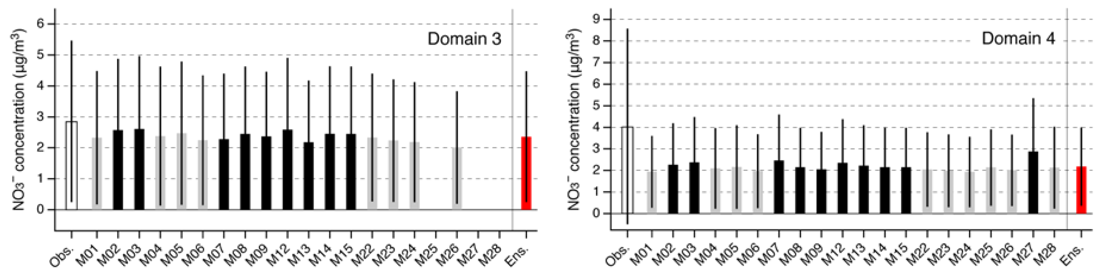
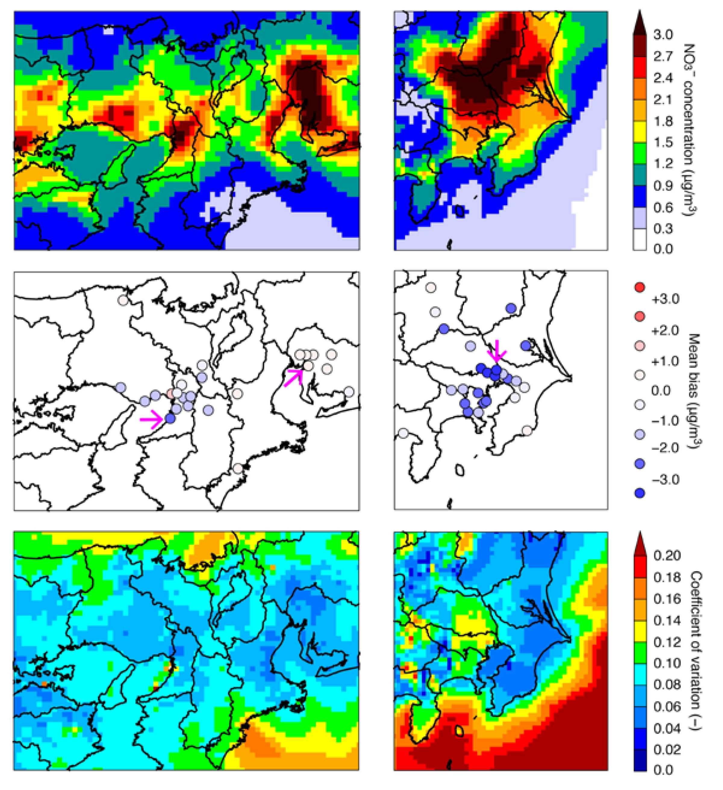
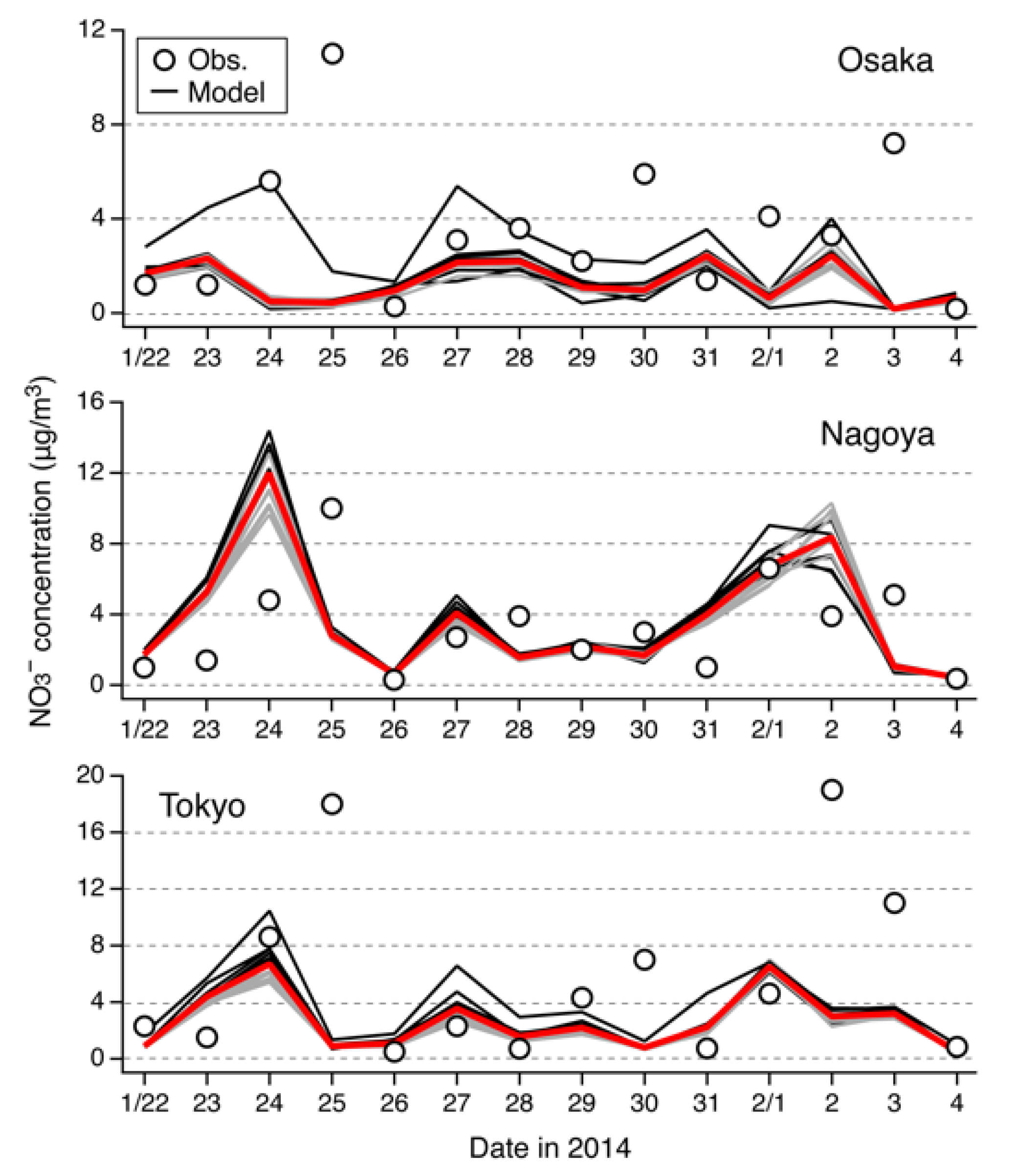
Overview of Model Performance

The spatial distribution of the observed NO₃⁻ concentration at APMSs averaged during winter are mapped in Figure 2. The observed NO₃⁻ concentration showed lower levels (i.e., less than 1.0 μg/m³) only at remote sites (e.g., near the edge of the domains), and the concentration level increased sharply (i.e., larger than 3.0 μg/m³) over the center of the Kansai and Kanto regions. The averaged concentration during winter across APMSs shown in Figure 2 over d03 and d04 are summarized in Figure 3. For the CMAQ models results, the Aitken, accumulation, and coarse modes were treated in the aerosol module, and the simulated hourly averaged concentration and the information about aerosol distributions taken in CMAQ after version 5.0 were used to calculate the concentrations so as that the distributions corresponded to the PM_2.5 observations. In contrast, the sum of Aitken and the accumulation modes was simply used for CMAQ version 4.7.1. Over d03, the averaged observed concentration was 2.8 μg/m³, and the concentrations in the models ranged from 2.0 to 2.6 μg/m³, indicating a slight underestimation. Over d04, the averaged observed concentration was 4.0 μg/m³, and the concentrations in the models ranged from 1.9 to 2.9 μg/m³. The models tended to underestimate the observed concentration, and the underestimation was larger over d04 than over d03.

In Figure 3, the model performance based on the ensemble mean are also shown. The ensemble mean was the simple average of all participating models:

$$\mathrm{Ensemble} \mathrm{Mean}=\frac{1}{N}{{\displaystyle \sum }}^{ }C$$

(1)

where C is the concentration simulated by each model and N is the number of models. N is 17 for d03 and 20 for d04 (see Table 1).

The performance of each model and the ensemble mean was determined from statistical analysis based on the correlation coefficient (R), normalized mean bias (NMB), normalized mean error (NME), mean fractional bias (MFB), and mean fractional error (MFE) (see Appendix A for their mathematical definitions). The values of R, NMB, and NME and the values of MFB and MFE were proposed in the model performance goal and performance criteria, respectively [38,39]. For NO₃⁻, R was not used to determine the model performance [38]. The proposed model performance goals were NMB <±15% and NME <+65% for the best model performance, and the proposed model performance criteria were NMB <±65% and NME <+115% for the acceptable model performance for daily NO₃⁻ concentration levels [38]. The model performance goals were also proposed as MFB $\le$±30% with MFE $\le$+50% for the best model performance, and the model performance criteria were proposed as MFB $\le$±60% with MFE $\le$+75% for acceptable model performance [39]. The performance of each model and model ensemble mean over d03 and d04 are summarized based on these judgements in

Table 2. Statistical analysis of model performances for NO₃⁻ over domains 3 and 4.

	R		NMB (%)				NME (%)				MFB (%)				MFE (%)
ID	d03	d04	d03		d04		d03		d04		d03		d04		d03	d04
M01	0.21	0.37	−18.7	*	−51.9	*	74.2	*	68.8	*	+2.9	**	−32.5	*	82.6	81.4
M02	0.16	0.29	−9.9	**	−43.9	*	79.8	*	70.3	*	+9.7	**	−19.9	**	87.1	83.3
M03	0.20	0.31	−8.6	**	−41.3	*	78.5	*	70.2	*	+9.7	**	−18.8	**	85.4	83.8
M04	0.16	0.29	−16.8	*	−48.0	*	79.0	*	70.9	*	+1.2	**	−28.6	**	87.6	84.1
M05	0.18	0.32	−13.5	**	−46.1	*	78.6	*	69.3	*	+4.4	**	−25.5	**	86.4	83.0
M06	0.19	0.32	−21.6	*	−51.3	*	75.3	*	69.9	*	−2.4	**	−32.5	*	85.6	83.4
M07	0.07	0.25	−20.4	*	−39.1	*	83.5	*	72.1	*	−0.8	**	−13.7	**	94.0	84.0
M08	0.19	0.30	−14.2	**	−46.9	*	76.5	*	69.5	*	+5.4	**	−25.0	**	84.9	82.4
M09	0.18	0.28	−16.9	*	−49.2	*	76.3	*	69.9	*	+3.5	**	−27.3	**	85.8	83.1
M12	0.18	0.30	−9.5	**	−41.8	*	79.1	*	69.8	*	+8.7	**	−18.2	**	86.0	83.0
M13	0.13	0.26	−23.9	*	−44.9	*	77.9	*	70.1	*	−5.2	**	−20.3	**	88.4	82.6
M14	0.19	0.30	−14.1	**	−46.9	*	76.5	*	69.5	*	+5.4	**	−25.0	**	85.0	82.4
M15	0.19	0.30	−14.2	**	−46.9	*	76.5	*	69.5	*	+5.4	**	−25.0	**	84.9	82.4
M22	0.20	0.31	−18.4	*	−49.4	*	74.6	*	69.3	*	+1.6	**	−28.5	**	84.1	81.7
M23	0.17	0.28	−21.9	*	−50.8	*	75.5	*	70.7	*	−1.7	**	−30.4	*	85.9	83.5
M24	0.17	0.28	−23.6	*	−52.1	*	74.9	*	70.8	*	−3.2	**	−32.2	*	85.8	84.0
M25	―	0.28	―		−47.1	*	―		69.6	*	―		−22.8	**	―	81.2
M26	0.14	0.24	−29.7	*	−50.3	*	75.5	*	71.0	*	−10.5	**	−27.4	**	87.1	82.9
M27	―	0.25	―		−28.7	*	―		73.7	*	―		−1.54	**	―	82.5
M28	―	0.24	―		−47.3	*	―		71.6	*	―		−25.8	**	―	83.7
Ens.	0.17	0.29	−17.4	*	−46.2	*	76.5	*	69.8	*	+2.7	**	−23.3	**	85.8	82.3

Note: Models simulated with the common dataset for domains 3 and/or 4 are shaded in grey (see, Table 1). ― denotes no submission for d03. ** Model performance goal. * Model performance criteria. See text for the details of these decisions.

.

The R values were around 0.2 over d03 and around 0.3 over d04, indicating that the linear correspondence between the models and observations was weak. The NMB of all models showed negative bias over d03 and d04 (Figure 3). NMB met the performance criteria over d03 and d04, and the scores were better over d03 compared to those over d04. Some models (M02, M03, M05, M08, M12, M14, and M15) showed the performance goal over d03. The M15 reference model achieved its NMB performance goal over d03. Despite the performance goal of M15 on NMB over d03, the performance of some other models showed the performance criteria on NMB over d03. This result suggested that even though the common dataset was used (i.e., M01, M04, M06, M22, M23, M24, and M26), the model performance could be worsened compared to the M15 reference model simulation; hence, the internal model settings in the model configuration should be considered. All models met the performance criteria for NME over d03 and d04, and the scores were slightly better over d04, in contrast to the results for NMB. This could have been related to the better R value over d04 compared with d03. The results for MFB were interesting. All models showed negative NMB values, whereas MFB showed positive or negative values over d03. Models M06, M07, M13, M23, M24, and M26 showed negative values for both NMB and MFB, and the NMB values were larger than for the other models, suggesting that these models tended to substantially underestimate the NO₃⁻ concentration. For all models, the MFE scores were above 80% and did not meet the model performance criteria.

The model performances were examined in terms of the horizontal distribution. The simulated horizontal distribution averaged during winter by the ensemble mean is shown in Figure 4 (top). Each model result is shown in Figures S1 and S2 in the supplementary material for d03 and d04, respectively. The mean bias between the ensemble mean and APMSs is spatially distributed in Figure 4 (center). Over remote areas (i.e., the edge of domain), the models performed well within a mean bias of −1.0 to +1.0 μg/m³. However, the model results were underestimated over central urbanized areas with intense emissions, especially in d04. To examine the model performance diversity, the coefficient of variation (CV) was calculated and is shown in Figure 4 (bottom). The CV is defined as the standard deviation among models divided by the model ensemble mean; therefore, a large value of CV indicates inconsistency among the models, whereas a small value indicates consistency. Only one grid over Osaka showed a large (i.e., greater than 0.30) CV over d03, and the value of CV was generally larger over the ocean rather than the land. This was the same over d04; the model differences in the south east in this domain (e.g., the Pacific Ocean) were large, and CV values between 0.12 and 0.18 were found over the Tokyo area. The value of CV was larger over the oceans, but the NO₃⁻ concentration over the ocean was smaller (i.e., below 1.0 μg/m³).

For a detailed analysis of the model performances, representative sites in Osaka, Nagoya, and Tokyo (indicated by pink arrows in Figure 2 and Figure 4) were investigated. Over Osaka, the site with the largest mean bias was found over southern Osaka and was selected. Over Nagoya, all models generally reproduced the NO₃⁻ concentration well and the mean bias was smaller; hence, the highest concentration site was chosen. Over Tokyo, the largest mean bias was found at a north-eastern site, which was selected. The temporal variation of the observations and all models including the ensemble mean are shown in Figure 5 at the three representative sites. At the Osaka site, the high concentration over 8 μg/m³ on 25 January was not simulated well by any of the models. This high concentration was also observed in Nagoya and Tokyo, and none of the models captured this high concentration either. At Osaka, one model (M03, discussed in detail in Section 4.1.2) showed a distinctly higher concentration and captured a high concentration on 24 January. At the Nagoya site, the model differences were smaller compared with the Osaka and Tokyo sites, and the model performance was better. At the Tokyo site, the high concentrations observed early on (25 January) and late in the analyzed period (2 February) were not well simulated by any of the models. Model performance differences were found in the early-to-middle part of the analyzed period. In summary, the models submitted to the first-phase of J-STREAM generally underestimated NO₃⁻ concentration, especially in d04 of the Kanto region; however, some models showed different behavior.

4. Discussion

In this section, each model setting is examined in detail, and we discuss the reasons for the different model behavior. In these comparisons, the difference between two models are defined as:

$$\mathrm{Difference}=C_{\mathrm{target}}-C_{\mathrm{reference}}$$

(2)

where, unless stated otherwise, C is the modelled NO₃⁻ concentration and M15 was used as a reference model. This calculation of the difference is shown as the time-averaged value over the analyzed period in winter. Before the model external and internal settings were examined, the dependence of the performance on the model version was investigated. The majority of the participating CMAQ versions were 5.1 and 5.0.2, and M05 and M15 were considered appropriate as reference models because these models used a common dataset and internal settings (Table 1). In the first-phase of J-STREAM, CMAQ version 5.0.1 was the main participating model; however, the changes in version 5.0.2 were minor. From CMAQ versions 5.0.2 to 5.1, several changes were introduced [40,41]. These updates included the species treated in the SAPRC07 chemical mechanism [42], the SOA treatment [43], and the description of clouds related to the inline calculation of the photolysis rate [44]. The difference between M05 and M15 is shown in Figure 6. Though the difference between M05 and M15 ranged from −0.2 to +0.3 μg/m³ in some grids, the spatially averaged difference was within ±0.1 μg/m³. Therefore, the model difference due to the model version was small (Figure 3), and the model differences caused by external and internal settings could play an important role. In Section 4.1 and Section 4.2, the model external and internal settings, respectively, are analyzed and discussed.

4.1. Investigation in Model External Settings

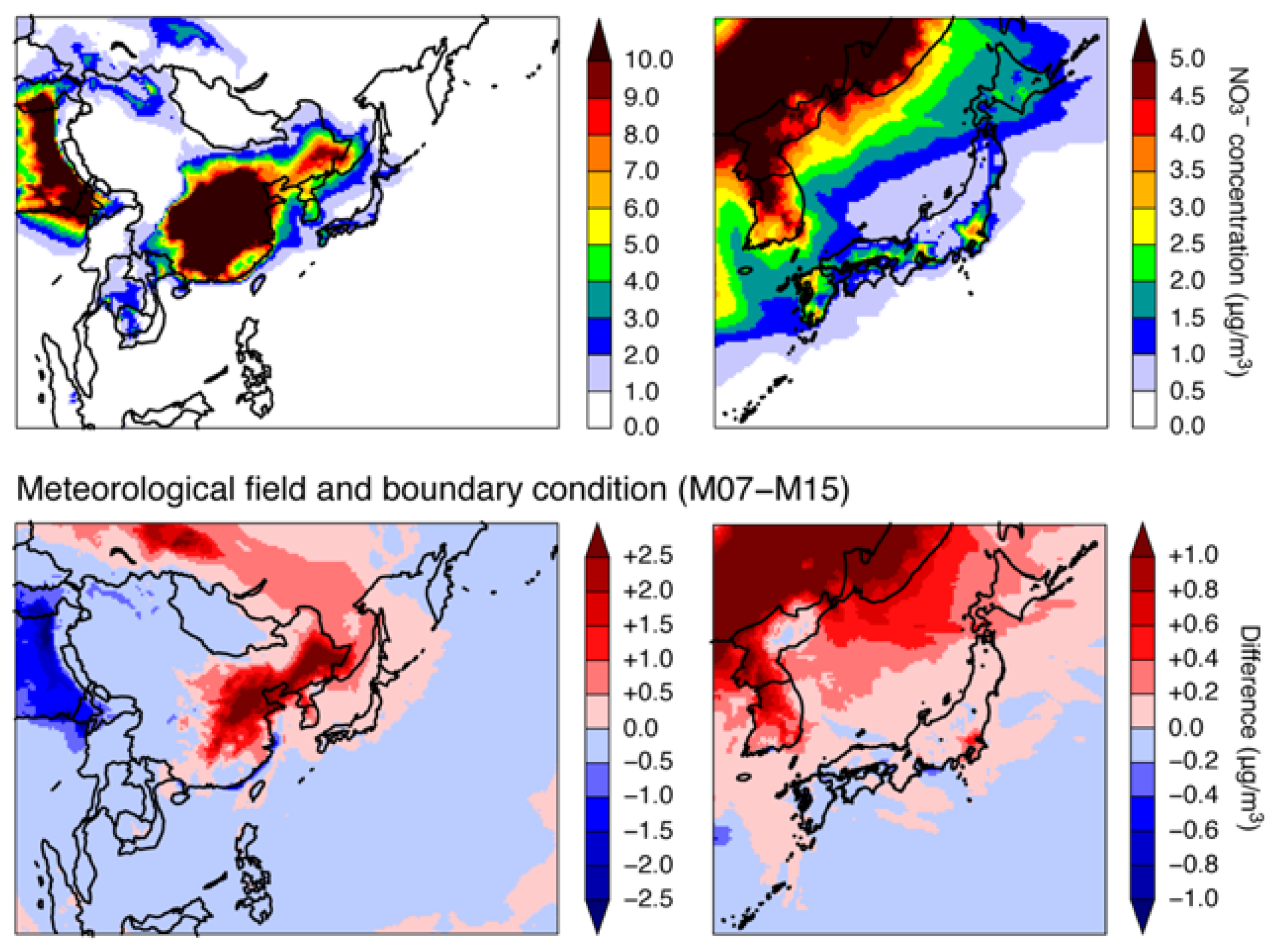
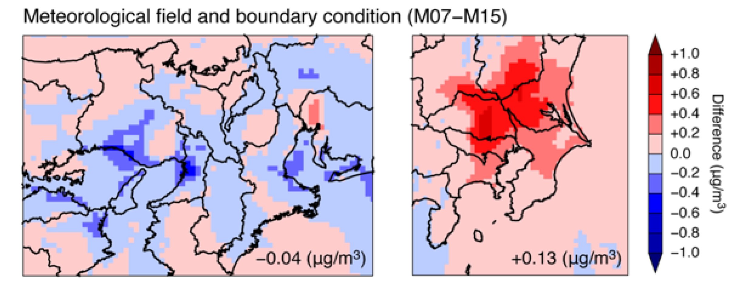
4.1.1. Meteorology and Boundary Conditions

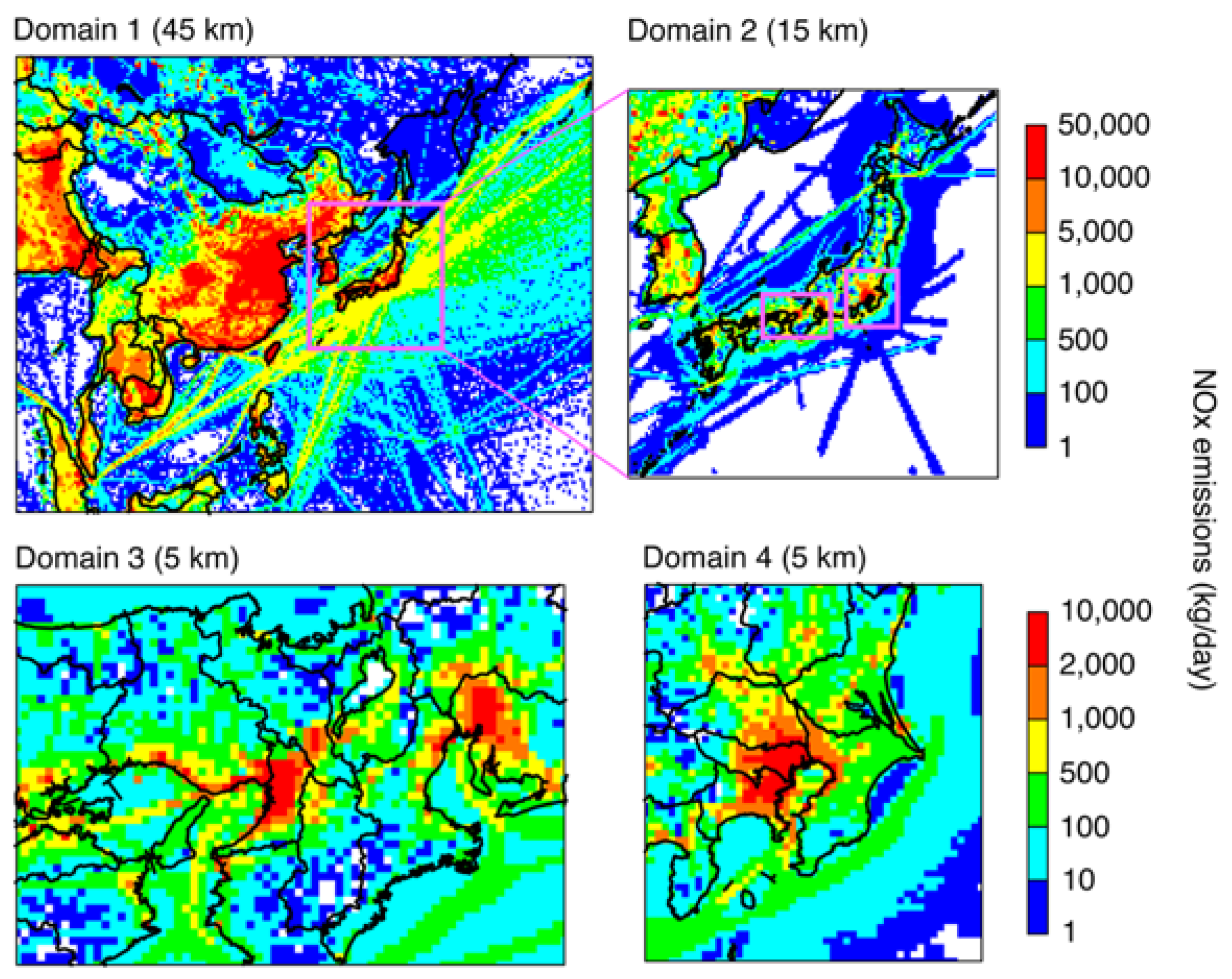
The model performance difference caused by the meteorology and boundary conditions could be seen by comparing M07 and the reference model M15 (see Table 1). This analysis was conducted from d01. In Figure 7, the modelled NO₃⁻ concentration in the M15 reference model is shown over d01 and d02, and the difference between M07 and M15 is also shown. Over Asia (d01), high NO₃⁻ concentrations above 10.0 μg/m³ (dark red in Figure 7) were limited to over the Asian continent (i.e., near intense emission sources) and low concentrations below 1.0 μg/m³ (white in Figure 7) were seen over most oceanic regions, except the East China Sea and the Sea of Japan. Over Japan (d02), high NO₃⁻ concentrations above 2.5 μg/m³ (yellow in Figure 7) were found over the western Japan, Kansai, and Kanto regions. The difference between M07 and M15 showed both effects caused by the meteorological field in different settings of the WRF meteorological model and boundary conditions taken from different global models. The effects near the boundaries of d01 were attributed mainly to the boundary conditions. Thus, the negative and positive differences over the western and northern edges of d01, respectively, stemmed from the effect of different global models. This difference was more than 1.0 μg/m³, and considering the low concentration level over the northern part of d01 (e.g., the far-east region of Russia), the selection of the global model will be an important setting for refining the model simulation over northern parts of the Asian continent. This point was also mentioned in the Asian-scale model inter-comparison study (MICS-Asia) [45,46]. Another possibility in addition to the aerosol components themselves was the difference caused by other species. For example, O₃ could have contributed to NO₃⁻ production, and M07 simulated higher O₃ during winter [8]; this difference might have been partly related to the difference found in NO₃⁻ in Figure 7.

The boundary condition and meteorological impact was further investigated by examining the differences between M07 and M15 over d03 and d04 (Figure 8). Over the Kansai region, the difference was sparsely found, whereas over the Kanto region, the difference was clearly visible as a higher concentration for M07 compared with M15 over the northern Tokyo area. The difference over the Kansai region was −0.5 to +0.3 μg/m³, and the spatially averaged difference was −0.04 μg/m³. In contrast, the difference over the Kanto region was mostly positive up to +0.7 μg/m³, and the spatially averaged value was +0.13 μg/m³. In terms of the meteorological field, the higher concentration found over the northern part of Tokyo was related to the characteristics of the land–sea breeze circulation over the Kanto region that transports high NO₃⁻ concentrations centered over Tokyo metropolitan area to the northern part of Tokyo. The role of the land–sea breeze is well known in summer [47]; however, the enhanced role in winter due to the urban heat island effect is caused by urbanization [48,49]. The meteorological field of the common dataset was evaluated for temperature, wind field, and precipitation in the overview paper [10], and it showed general agreement. An examination of different meteorological fields itself is required, and the behavior of NO₃⁻ caused by the meteorological field could be one of the key points for further study. In addition, the difference caused by the meteorological field and boundary conditions should be separately investigated in further studies to distinguish their respective impact over the urban area of Japan.

4.1.2. Emission

The model performance difference caused by emissions can be examined in M03 and M27, with M15 as the reference model (see Table 1). Models M03 and M27 performed differently; in particular, the bias (NMB and MFB) performance scores were better than in the other models (Table 2). Therefore, the emission external setting was one of the most important factors in the model differences. M03 and M15 were compared over d03, and M03, M15, and M27 were compared over d04. The differences in NO₃⁻ concentration and relevant emissions and chemical species are presented in Figure 9 for d03 and Figure 10 for d04.

Over d03, the model performance difference for NO₃⁻ concentration was inhomogeneous, but M03 gave higher concentrations over most parts of Osaka and a slightly higher concentration over Nagoya (Figure 9a). The difference ranged from −0.9 to +2.5 μg/m³, and the spatially averaged difference was +0.10 μg/m³ due to the inhomogeneous difference over d03. Figure 9a illustrates the temporal variation for M03 and M15 at the two representative sites in Osaka and Nagoya shown in Figure 5. The performance of M03 at the Osaka site was distinct. For example, on 24 January, all models gave concentrations close to zero, except for M03, which simulated a concentration of 6.0 μg/m³ to capture the observation. As in d03, M03 also gave a higher concentration over d04 (Figure 9a). The difference between M03 and M15 ranged from −0.4 to +0.8 μg/m³, and the spatially averaged difference was +0.16 μg/m³. Furthermore, compared with M03, M27 gave higher concentrations (Figure 10a). The difference between M27 and M15 ranged from −0.5 to +1.8 μg/m³, and the spatially averaged difference was +0.49 μg/m³. The temporal variations of NO₃⁻ concentration at Tokyo for M03, M15 and M27 are also shown in Figure 10a. Over d04, as indicated by the comparison across APMSs (Table 2 and Figure 3), M27 simulated higher NO₃⁻ concentrations than M03.

Over d03 and d04, we investigated the related species to explain the difference in model performance in NO₃⁻ concentration. NO_x emissions were higher in M15 than in both M03 and M27 over d03 and d04, (Figure 9b and Figure 10b), and as a sequence, NO_x concentration was higher in M15 than in M03 and M27 (Figure 9c and Figure 10c). Comparing the daily averaged observed NO_x concentration showed that the higher concentration simulated by M15 matched the observations better. The NO₃⁻ precursors, HNO₃ and NH₃ gas, were examined further. The difference in HNO₃ concentration between M03 or M27 and M15 was small (Figure 9d and Figure 10d)—mostly within −0.3 to +0.3 ppbv over the whole of d03 and d04. Therefore, the difference in NO₃⁻ concentration could be associated with NH₃ behavior. The difference in NH₃ emissions (the NH₃ emissions of the common dataset are shown in Figure S3 in supplementary material) was inhomogeneous (Figure 9e and Figure 10e); however, higher NH₃ emissions in M03 and M27 were found over Osaka and Tokyo, where higher NO₃⁻ concentrations were also observed. Despite these higher NH₃ emissions, NH₃ concentrations were mostly lower in M03 and M27 than in M15.

In terms of the configuration of M03 and M27, these model versions were different from the M15 reference model (Table 1). The difference between M03 and M02, and M27 and M28 were solely attributed to the difference due to emissions originally used as the difference dataset from the common dataset. These additional analyses are shown in Figures S4 and S5 in the supplementary material. The differences found as spatial distributions were generally similar to those found from the difference to M15, and the timeseries of M02 and M28 were closer to M15 rather than M03 and M28, respectively. As discussed in the introduction of Section 4, the difference due to the model version could have been small, and the differences that arose from the model external settings (i.e., emissions in this case) would have led to large model performance differences.

This behavior was examined in detail based on the gas ratio (GR) analysis [50]. The GR indicated the sensitivity of NO₃⁻ to changes in SO₄²⁻ and NH₄⁺ concentration. For the SO₄²⁻ concentration, the SO₂ emissions in the common dataset are shown in Figure S6, and the model performances are presented in Figures S7 and S8 in the supplementary material for SO₄²⁻ and SO₂ in the same format as in Figure 9 and Figure 10. The GR is defined as the ratio of free ammonia to the total nitrate as:

$$\mathrm{GR}=\frac{\left[{\mathrm{NH}}_3+{\mathrm{NH}}_4^{+}\right]-2\times \left[{\mathrm{SO}}_4^{2-}\right]}{\left[{\mathrm{HNO}}_3+{\mathrm{NO}}_3^{-}\right]}$$

(3)

where it is assumed that SO₄²⁻ is fully neutralized, as indicated by the coefficient of 2 for [SO₄²⁻]. This formulation can be extended more accurately as the adjusted gas ratio (adjGR) by introducing the degree of sulfate neutralization (DSN):

$$\mathrm{adjGR}=\frac{\left[{\mathrm{NH}}_3+{\mathrm{NH}}_4^{+}\right]-\mathrm{DSN}\times \left[{\mathrm{SO}}_4^{2-}\right]}{\left[{\mathrm{HNO}}_3+{\mathrm{NO}}_3^{-}\right]}$$

(4)

The DSN is defined as:

$$\mathrm{DSN}=\frac{\left[{\mathrm{NH}}_4^{+}\right]-\left[{\mathrm{NO}}_3^{-}\right]}{\left[{\mathrm{SO}}_4^{2-}\right]}$$

(5)

where the DSN is equal to or greater than 2 if there is sufficient NH₄⁺. As a result, the adjGR in Equation (4) is expressed as:

$$\mathrm{adjGR}=\frac{\left[{\mathrm{NH}}_3\right]+\left[{\mathrm{NO}}_3^{-}\right]}{\left[{\mathrm{HNO}}_3\right]+\left[{\mathrm{NO}}_3^{-}\right]}$$

(6)

The adjGR value was used to understand the NO₃⁻ production conditions; an adjGR value greater than 1 means that NH₃ is abundant for neutralizing both SO₄²⁻ and NO₃⁻ (NH₃-rich).

The spatial distribution patterns of adjGR are plotted in Figure 11. During the analyzed period, high NO₃⁻ concentrations generally greater than 1.5 μg/m³ (yellow in Figure 4, or Figures S1 and S2) corresponded well to NH₃-rich conditions. Therefore, under NH₃-rich conditions, the consumption of NH₃ was larger in M03 and M27 than in M15, and this led to higher NO₃⁻ concentrations. Due to the effective consumption of NH₃, the value of adjGR was lower in M03 and M27 than in M15; however, the NH₃-rich conditions suggested by adjGR being equal to unity was similar in M03, M27, and M15. The analysis of the differences in emissions revealed that the differences in NO₃⁻ concentration were caused by emission settings for NH₃ emissions rather than NO_x emissions.

4.2. Investigation in Internal Model Settings

4.2.1. Chemical Mechanism

The chemical mechanisms were configured differently in the submitted CMAQ models in the first-phase of J-STREAM, and it was appropriate to compare models M08, M09, M12, and M13 because the model performance difference caused by the chemical mechanism for O₃ concentration of these four models was previously analyzed [9]. Therefore, the model performance difference caused by the chemical mechanism was examined in M08, M09, M12, and M13, and M13 was used as a reference model in this case because the SAPRC99 used in M13 was the oldest mechanism and the differences could be interpreted as the progress related to updating the mechanisms. Due to the restriction of the selection of the aerosol module, the M13 of SAPRC99 was configured with AERO5, whereas other models of M08, M09, and the M12 of SAPRC07, CB05, and RACM2 were configured with AERO6 (Table 1). The differences are shown in Figure 12 over all domains. Over d01, SAPRC07 (M08) showed a higher NO₃⁻ concentration compared with SAPRC99 (M13) over southern China, but it showed a lower concentration over India. The comparison between CB05 (M09) and SAPRC99 (M13) showed complex differences with a higher NO₃⁻ concentration in CB05 over southern China and a lower concentration over northern China and India. RACM2 (M12) mostly gave higher NO₃⁻ concentrations than SAPRC99 (M13). The higher concentration in RACM2 was consistent with the results over Europe and the U.S. [51,52]. The difference of precursors of HNO₃ and NH₃ were analyzed and presented in Figure S9 in the supplementary material. The dependencies on HNO₃ and NH₃ showed a complex feature; higher concentration by M08 and M09 were related to NH₃, whereas that by M12 depended on HNO₃. Over d02, the difference in China affected western Japan and could have been related to the NO₃⁻ concentrations over d03 of the Kansai region. The difference caused by chemical mechanisms over western Japan was up to +1.0 μg/m³, and this impact occurred over a broad area over western Japan. Over d03, the difference in chemical mechanisms was mostly positive compared with SAPRC99, and the differences between SAPRC07 and SAPRC99 (M08 and M13), CB05 and SAPRC99 (M09 and M13), and RACM2 and SAPRC99 (M12 and M13) were all up to +0.8 μg/m³. The spatial averaged differences were +0.23, +0.22, and +0.26 μg/m³ for SAPRC07, CB05, and RACM2, respectively, compared with SAPRC99. From this analysis, we concluded that the difference due to the chemical mechanisms could have an effect, especially over western Japan and the Kansai region, and this difference may have been mostly related to the long-range transport from outside of Japan. However, the difference related to the long-range transport was not found over d04 of the Kanto region. As seen in d02, the sequential difference from the Asian continent did not reach the Kanto region. The behavior of the difference in NO₃⁻ concentration over the Kanto region was different, especially for CB05, which showed a negative difference over northern Tokyo. The difference between SAPRC07 and SAPRC99 (M08 and M13) ranged from −0.2 to +0.3 μg/m³, the difference between CB05 and SAPRC99 (M09 and M13) ranged from −0.3 to +0.4 μg/m³, and the difference between RACM2 and SAPRC99 (M12 and M13) was up to +0.3 μg/m³. The spatial averaged differences were +0.09, +0.08, and +0.12 μg/m³ for SAPRC07, CB05, and RACM2, respectively, compared with SAPRC99. Over the Kanto region, the difference due to the chemical mechanism was limited, and its effects were smaller compared with those over the Kansai region.

4.2.2. KZMIN

In CMAQ models, the minimum eddy diffusivity was set as 1.0 m² s⁻¹; however, when the user used the KZMIN option, the minimum eddy diffusivity was internally calculated below an assigned altitude (500 m) as:

$$\mathrm{Minimum}{K}_z=K_z\left(\mathrm{lower}\right)+\left(K_z\left(\mathrm{upper}\right)-K_z\left(\mathrm{lower}\right)\right)\times \mathrm{PURB},$$

(7)

where $K_z\left(\mathrm{lower}\right)$ is 0.01 m² s⁻¹, $K_z\left(\mathrm{upper}\right)$ is 1.0 m² s⁻¹, and the variation of PURB is the percentages of the urban fraction derived from the land use data. Therefore, when the KZMIN option was used, the minimum eddy diffusivity for grids categorized as urban areas could be lower than the prescribed value of 1.0 m² s⁻¹, and the minimum eddy diffusivity was reduced to 0.01 m² s⁻¹ at the grids for nonurban areas [40]. Before version 5.0 (version 4.7.1 was used in this study), the values used for $K_z\left(\mathrm{lower}\right)$ and $K_z\left(\mathrm{upper}\right)$ were different and were 0.5 and 2.0 m² s⁻¹, respectively.

In the model settings submitted to J-STREAM, it was not possible to directly compare the KZMIN option, but M06 and M23 could be used to investigate the difference caused by the KZMIN option despite the differences in the model version. M26 and M28 could also be used; however, because of the changes in the $K_z\left(\mathrm{lower}\right)$ and $K_z\left(\mathrm{upper}\right)$ values before and after version 5.0, M26 and M28 were not compared. Before M06 and M23 were compared, the difference between M05 and M22 was checked to investigate the difference caused by updating the model version (see also Figure 6). The difference between M05 and M22 showed a slightly higher NO₃⁻ concentration for M05, especially over Nagoya and northern Tokyo (Figure 13). The difference ranged from −0.1 to +0.4 μg/m³ over d03 and from −0.1 to +0.4 μg/m³ over d04. The spatial averaged difference was +0.04 μg/m³ over d03 and +0.08 μg/m³ over d04, indicating that the difference due to the model version was small.

In the comparison of M06 and M23, the updated photolysis rate in the model version could be neglected because both models used a look-up table to calculate the photolysis rate. The PURB mapping used in this study and the difference between M06 and M23 are shown in Figure 14. Higher PURB values were seen over Osaka and Tokyo. Despite the model version difference, this result suggested that the KZMIN option could cause a lower NO₃⁻ concentration over urban areas and a higher NO₃⁻ concentration over nonurban areas. However, the difference ranged from −0.3 to +0.4 μg/m³ over d03 and from −0.2 to +0.2 μg/m³ over d04, and the spatial averaged differences were below +0.05 μg/m³ over both domains. The effect of the treatment of KZMIN has been reported for night time O₃ formation [53]. For the further study of the effects of KZMIN, the daily averaged value is insufficient, and observations with high temporal resolution are required [54]. This analysis could be included in the second-phase of J-STREAM using hourly observations of inorganic aerosols [55]. Moreover, as the land use data in the first-phase of J-STREAM were based on the United States Geological Survey (USGS), urban areas were underrepresented compared with the observations. Therefore, the second-phase of J-STREAM has established a new land use dataset, and the meteorological field, biogenic emissions, and concentrations of O₃ and SOA in this revision have been verified [7].

4.2.3. HONO and Photolysis

The CMAQ models contain the HONO option. In general, HONO is produced in the atmosphere by a direct emission, gas phase oxidation, heterogeneous reaction, and by a surface photolysis reaction. The HONO option in CMAQ models controls whether the heterogeneous reaction is considered [35]. In several heterogeneous reactions involving HONO, the following reaction is the most important:

$$2{\mathrm{NO}}_2+{\mathrm{H}}_2\mathrm{O}\to \mathrm{HONO}+{\mathrm{HNO}}_3$$

(8)

This heterogeneous reaction could occur on aerosol and ground surfaces and is implemented in CMAQ models with a first-order rate constant in NO₂ [35]. This production of HNO₃ will lead to the formation of NO₃^- via the gas phase reaction with NH₃. The HONO reaction is also related to photolysis; however, there have been updates to the inline calculation of photolysis along with model updates (see Section 4.2.2). Therefore, distinguishing the effects of each change is difficult. The differences in NO₃⁻ concentration due to the model external and internal settings are shown in Figure 15.

The model performance differences in NO₃⁻ concentration due to the model external settings (opaque colors in Figure 15) were greater than those due to the model internal settings (transparent colors in Figure 15 with gray texts). The detail of the model external settings have been discussed in Section 4.1. In the results for the model internal settings, SAPRC99 tended to simulate lower NO₃⁻ concentrations than other chemical mechanisms (see Section 4.2.1). For example, the domain-averaged value showed a higher NO₃⁻ concentration in M06, in which KZMIN was used, than in M23 (see Section 4.2.2). Here, we focus on HONO and the photolysis options. The selection of the HONO option caused better model performance in terms of the HONO concentration. The models M04, M06, M23, M24, M26, M27, and M28, in which the HONO option was switched off, simulated a HONO concentration five times lower than the other models, which included the HONO heterogeneous reaction. The spatial distributions of the models are shown in Figures S10 and S11 in the supplementary material over d03 and d04, respectively. Models in which the HONO option was switched off simulated HONO concentrations of 0.01–0.02 pbbv, whereas models including the HONO option simulated concentrations of up to 0.5 ppbv over d03 and d04. The observed HONO concentration over Nara prefecture, which is close to Osaka, was 0.58–1.26 ppbv during the 1994–1995 winter season [56]. In addition, the HONO concentration observed at Tsukuba, which is a rural area in the Kanto region, was 0.86 ± 0.14 ppbv during the 2004–2005 winter season [57]. Based on this qualitative comparison with the HONO observation, the simulated HONO concentrations without the heterogeneous reaction were an order of magnitude too low, and we concluded that the HONO option should be switched on in the simulation settings over Japan.

The photolysis calculation is involved in reactions of the reactive nitrogen (e.g., NO₂, NO₃, HONO, and HNO₃) and other important species such as O₃. In the comparison of the photolysis methods, the inline calculation (circles in Figure 15) was generally related to higher NO₃⁻ concentrations, except for M13, which was configured with the SAPRC99 model. The models M06, M23, M24, M26, M27, and M28 used a lookup table (triangles in Figure 15), and these models also switched off the HONO option. The model performances of M01, M04, M06, M22, M23, M24, and M26 using the common dataset were worse over d03 compared with the M14 reference model. In principle, the table option for photolysis calculated the daily clear-sky photolysis rates from the look-up tables of molecular absorption cross-sections and quantum yield data, as well as climatologically-derived O₃ column and optical depth data. In contrast, the inline option for photolysis accounted for the presence of O₃ and ambient aerosol predicted in the CMAQ model and used these estimates to adjust the actinic flux, rather than relying on a look-up table. This could be realistic calculation but it also included errors associated with the simulation results. In addition, the cloud distribution and optical properties are described more consistently in the meteorological field following the updates after version 5.1 [44]. Therefore, inline photolysis calculations are theoretically reasonable. The analysis shown in Figure 15 shows that the HONO option and inline photolysis calculations should be used to simulate higher NO₃⁻ concentrations over urban areas in Japan.

5. Conclusions

The first-phase of the Japanese model inter-comparison study, J-STREAM, found that NO₃⁻ was underestimated during winter. In the present study, the reason for this model underestimation was analyzed by focusing on CMAQ, and the external and internal model settings were investigated over urban areas in Japan, namely, the Kansai (e.g., Osaka and Nagoya) and Kanto (e.g., Tokyo) regions. The findings are summarized as follows.

• Boundary conditions and meteorology external settings: The difference due to different boundary conditions for the outermost domain and meteorological field ranged from −0.5 to +0.3 μg/m³ (−0.04 μg/m³; hereafter, the domain average is shown in parenthesis) over the Kansai region. In contrast, a different meteorological field showed higher NO₃⁻ concentrations over the Kanto region of up to +0.7 μg/m³ (+0.13 μg/m³). This could have been related to the land–sea breeze circulation in the Kanto region. The factor of boundary condition and meteorology need to be investigated separately in future study, and further investigation of the effects of several meteorological fields should be performed.
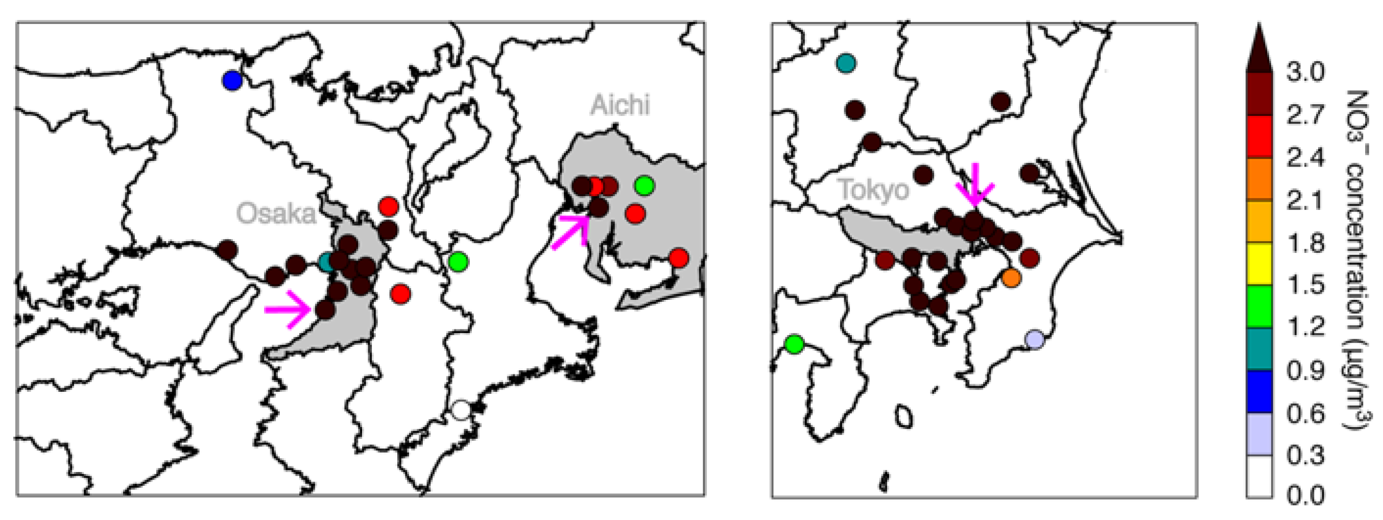
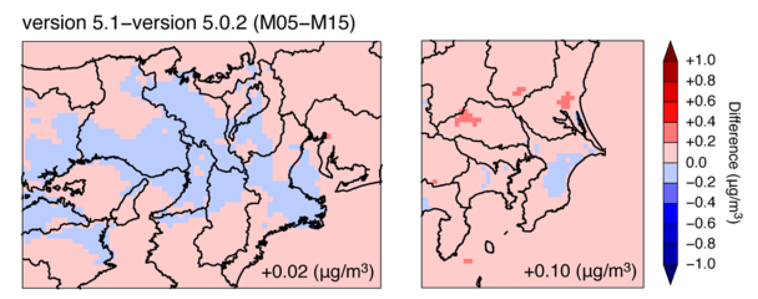
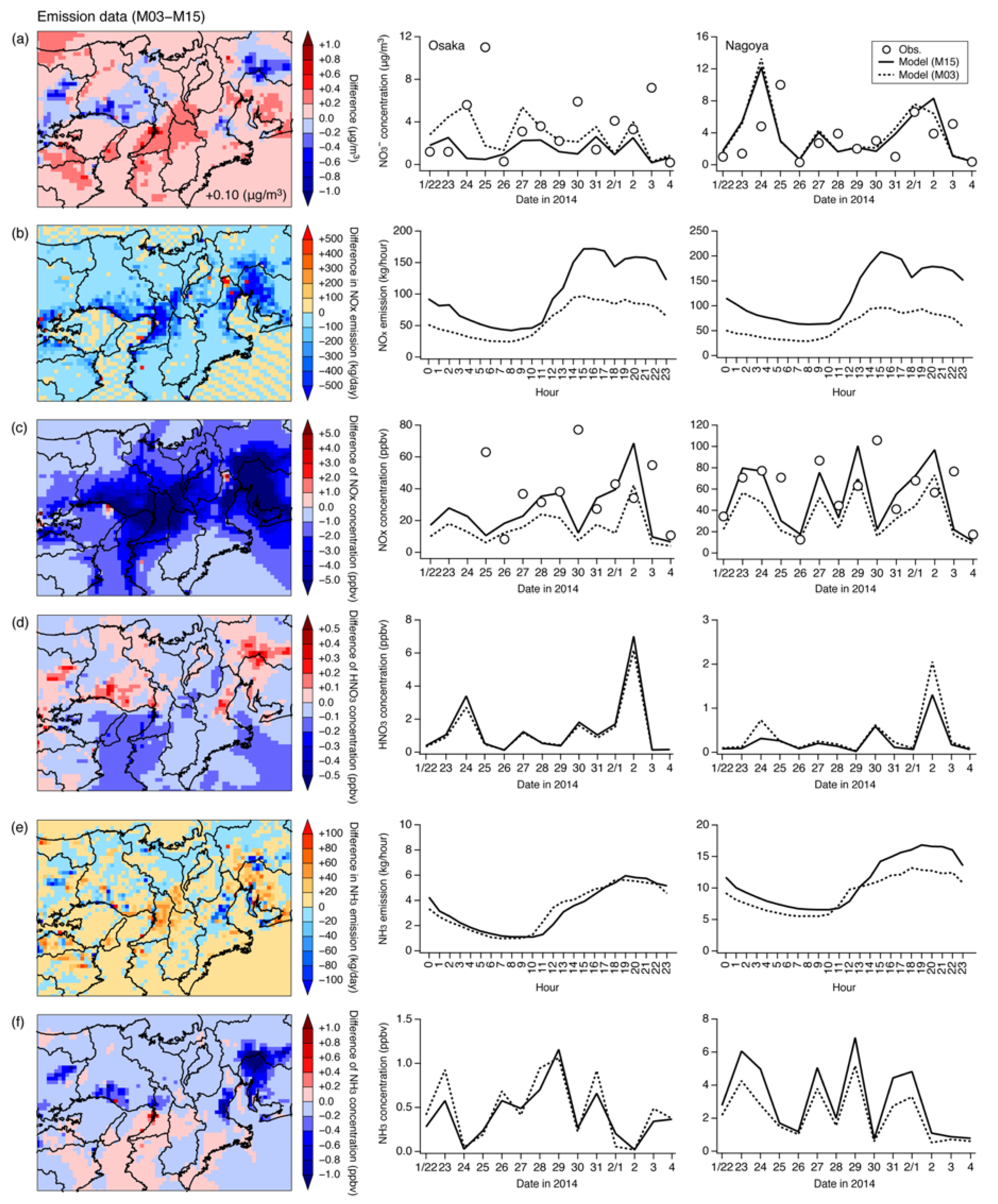
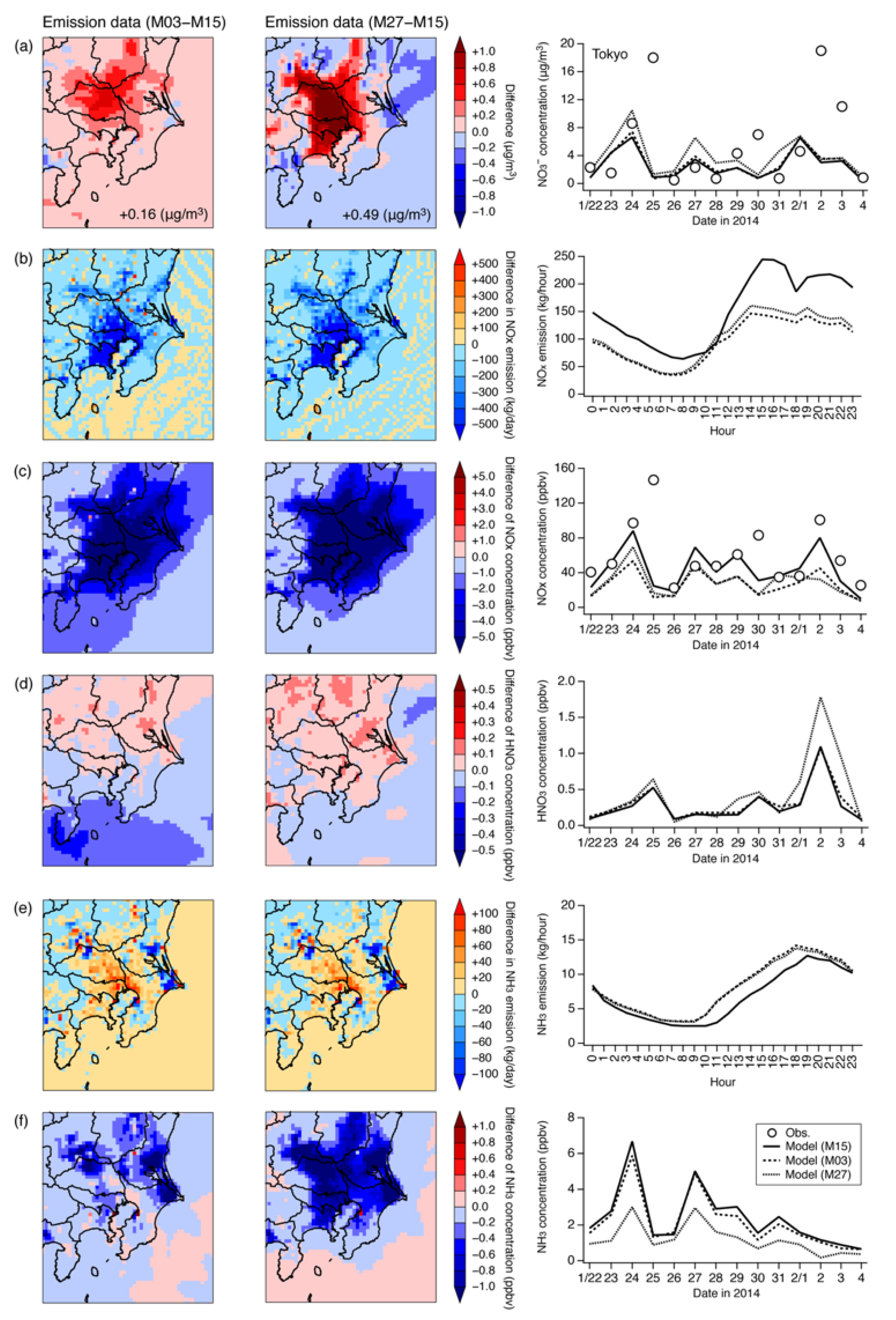
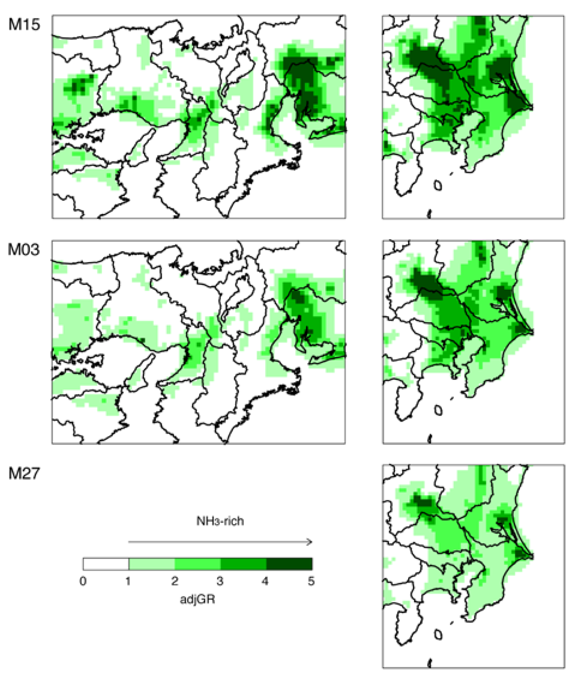
• Emissions external setting: Using different emissions led to higher NO₃⁻ concentrations over the Kansai region in one model and over the Kanto region in two models. Over the Kansai region, the difference ranged from −0.9 to +2.5 μg/m³ (+0.10 μg/m³). Over the Kanto region, these differences ranged from −0.4 to +0.8 μg/m³ (+0.16 μg/m³) and from −0.5 to +1.8 μg/m³ (+0.49 μg/m³). The different emissions were obtained with lower NO_x emissions and higher NH₃ emissions. The effective consumption under NH₃-rich conditions over urban areas in Japan was related to the higher production of NO₃⁻.
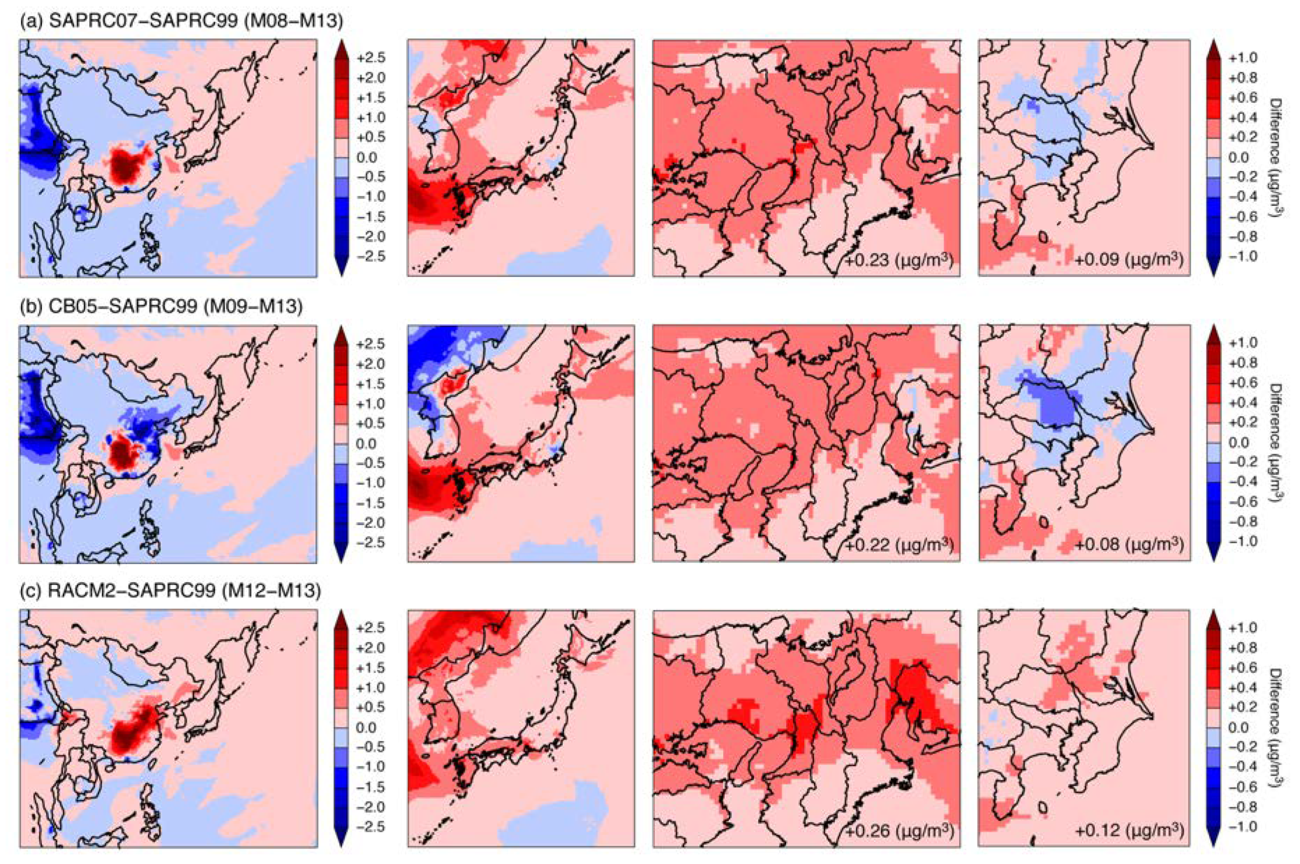
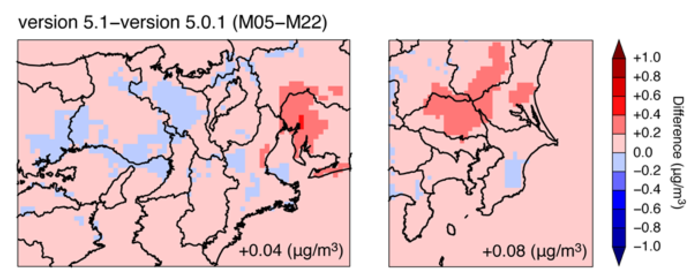
• Chemical mechanism internal setting: SAPRC99 showed a lower NO₃⁻ concentration compared with SAPRC07, CB05, and RACM2. The different chemical mechanisms caused a large difference over China, and this could affect western Japan and the Kansai region. The effect of the chemical mechanisms over western Japan was up to +1.0 μg/m³. Over the Kansai region, the difference between SAPRC07 and SAPRC99 was up to +0.8 μg/m³ (+0.23 μg/m³), that between CB05 and SAPRC99 was up to +0.8 μg/m³ (+0.22 μg/m³), and that between RACM2 and SAPRC99 was up to +0.8 μg/m³ (+0.26 μg/m³). In contrast, over the Kanto region, the difference between SAPRC07 and SAPRC99 was −0.2 to +0.3 μg/m³ (+0.09 μg/m³), the difference between CB05 and SAPRC99 was −0.3 to +0.4 μg/m³ (+0.08 μg/m³), and the difference between RACM2 and SAPRC99 was up to +0.3 μg/m³ (+0.12 μg/m³). The selection of the chemical mechanism could increase NO₃⁻ concentration over western Japan via long-range transport, and the difference over the Kanto region was smaller.
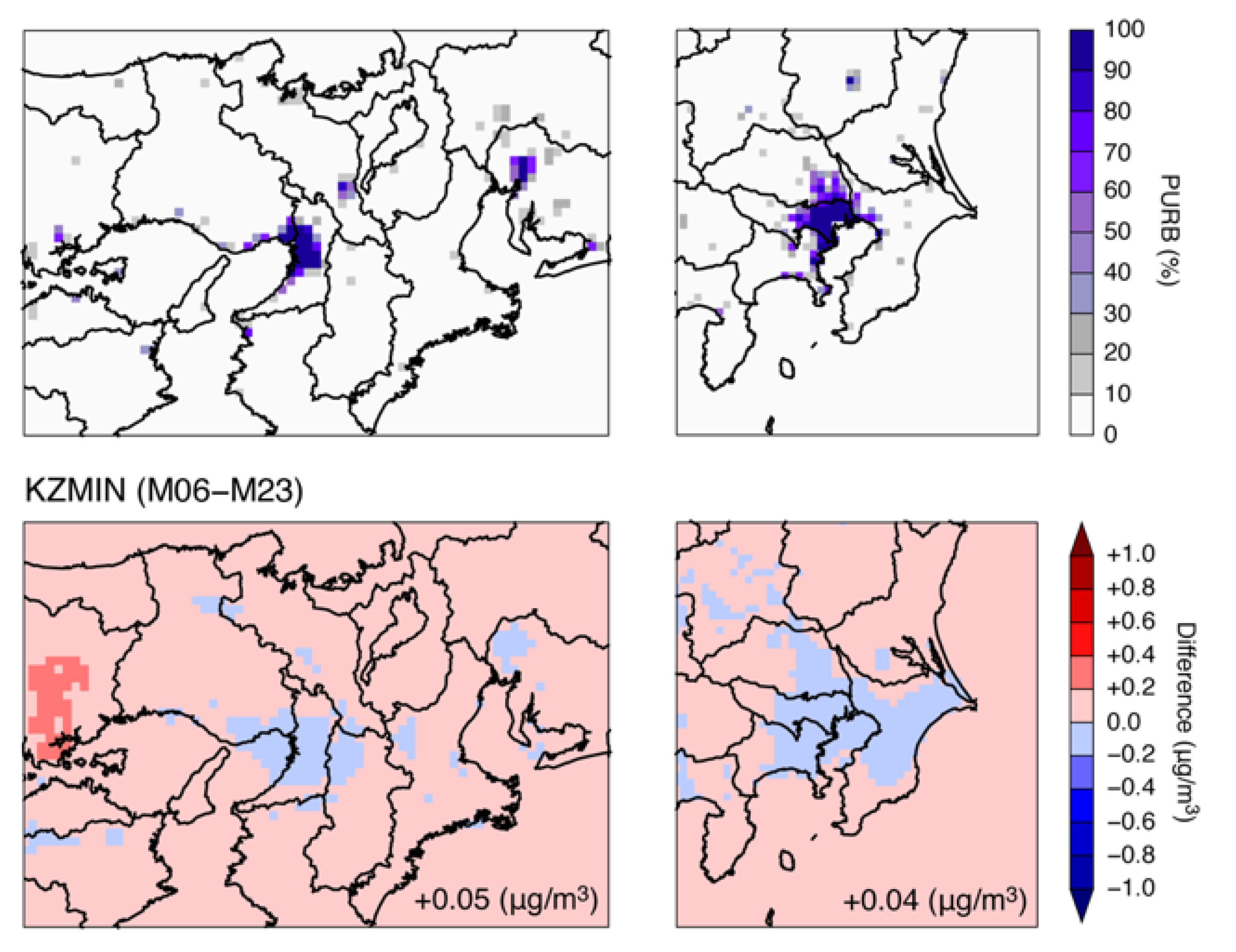
• KZMIN internal setting: The use of the KZMIN option, which calculates lower minimum vertical diffusion coefficients compared with the prescribed value, led to lower concentrations over the grids with a land use category of urban, as well as to higher concentration over other grids. Though there was a clear relation between the difference and the fraction of urban area, these differences over domains 3 and 4 (+0.05 and +0.04 μg/m³, respectively) were smaller.
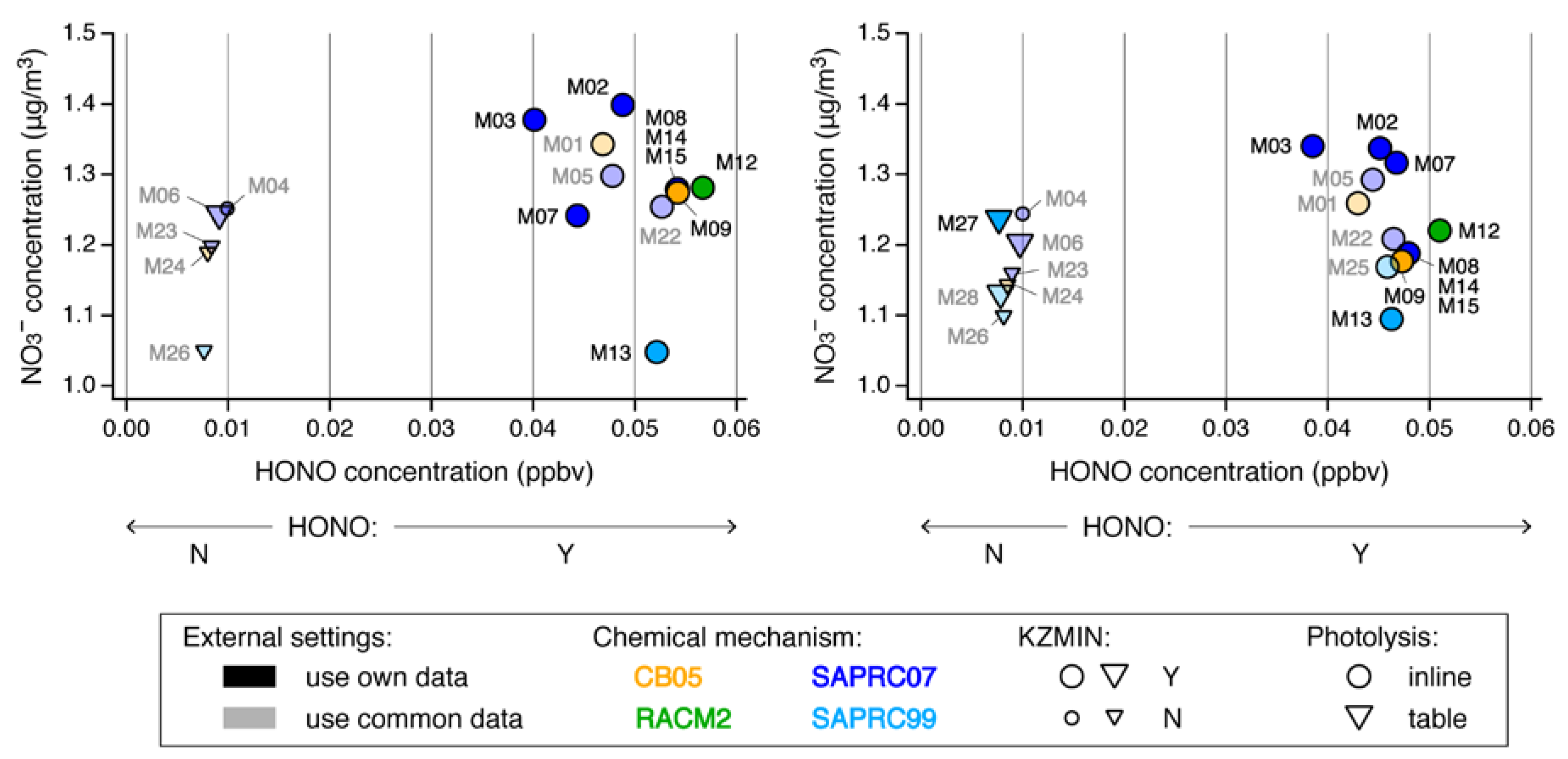
• HONO and photolysis internal settings: The models in which the HONO option was switched off, including the heterogeneous reaction of HONO, showed a HONO concentration five times lower than in models with the option switched on. Based on the comparison with HONO observations in Japan, the HONO concentration simulated by models without the heterogeneous reaction were an order of magnitude too low. Some models also used a lookup table to calculate photolysis. The difference in model performance between these models and the M15 reference model suggested that the HONO option should be switched on and that inline photolysis calculation is required for simulating air quality over urban areas in Japan.

In further studies, different external settings as potential factors to cause large differences on modeling performance rather than internal settings should be investigated. In this study, the observations were based on daily averaged values; however, these are inadequate for understanding the diurnal variation closely related to meteorology, emissions, and other factors. Comparisons with high-temporal resolution measurements are being examined in the second-phase of J-STREAM [54]. As the KZMIN option showed different behavior on urban and nonurban grids, simultaneous measurements at different locations in the Kanto region could improve our understanding of the behavior of air pollutants over urban and nonurban areas [58].

References

1. Carmichael, G.R.; Sandu, A.; Chai, T.; Daescu, D.N.; Constantinescu, E.M.; Tang, Y. Predicting air quality: Improvements through advanced methods to integrate models and measurements. J. Comp. Phys. 2008, 227, 3540–3571. [Google Scholar] [CrossRef]
2. Morino, Y.; Chatani, S.; Hayami, H.; Sasaki, K.; Mori, Y.; Morikawa, T.; Ohara, T.; Hasegawa, S.; Kobayashi, S. Inter-comparison of chemical transport models and evaluation of model performance for O3 and PM2.5 prediction—Case study in the Kanto area in summer 2007. J. Jpn. Soc. Atmos. Environ. 2010, 45, 212–226. (In Japanese) [Google Scholar]
3. Chatani, S.; Morino, Y.; Shimadera, H.; Hayami, H.; Mori, Y.; Sasaki, K.; Kajino, M.; Yokoi, T.; Morikawa, T.; Ohara, T. Multi-model analyses of dominant factors influencing elemental carbon in Tokyo metropolitan area of Japan. Aerosol Air. Qual. Res. 2014, 14, 396–405. [Google Scholar] [CrossRef] [Green Version]
4. Shimadera, H.; Hayami, H.; Chatani, T.; Morino, Y.; Mori, S.; Morikawa, Y.; Yamaji, K.; Ohara, T. Sensitivity analyses of factors influencing CMAQ performance for fine particulate nitrate. J. Air Waste Manag. 2017, 64, 374–387. [Google Scholar] [CrossRef] [PubMed] [Green Version]
5. Shimadera, H.; Hayami, H.; Chatani, S.; Morikawa, T.; Morino, Y.; Mori, Y.; Yamaji, K.; Nakatsuka, S.; Ohara, T. Urban air quality model inter-comparison study in Japan (UMICS) for improvement of PM2.5 simulation in greater Tokyo area of Japan. Asian J. Atmos. Environ. 2018, 12, 139–152. [Google Scholar] [CrossRef]
6. Chatani, S.; Yamaji, K.; Sakurai, T.; Itahashi, S.; Shimadera, H.; Kitayama, K.; Hayami, H. Overview of model inter-comparison in Japan’s study for reference air quality modeling (J-STREAM). Atmosphere 2018, 9, 19. [Google Scholar] [CrossRef] [Green Version]
7. Chatani, S.; Okumura, M.; Shimadera, H.; Yamaji, K.; Kitayama, K.; Matsunaga, S. Effects of a detailed vegetation database on simulated meteorological fields, biogenic VOC emissions, and ambient pollutant concentrations over Japan. Atmosphere 2018, 9, 179. [Google Scholar] [CrossRef] [Green Version]
8. Chatani, S.; Yamaji, K.; Itahashi, S.; Saito, M.; Takigawa, M.; Morikawa, T.; Kanda, I.; Miya, Y.; Komatsu, H.; Sakurai, T.; et al. Identifying key factors influencing model performance on ground-level ozone over urban areas in Japan through model-intercomparisons. Atmos. Environ. 2020, 223, 117255. [Google Scholar] [CrossRef]
9. Kitayama, K.; Morino, Y.; Yamaji, K.; Chatani, S. Uncertainties in O3 concentrations simulated by CMAQ over Japan using four chemical mechanisms. Atmos. Environ. 2019, 198, 448–462. [Google Scholar] [CrossRef]
10. Yamaji, K.; Chatani, S.; Yamaji, K.; Itahashi, S.; Saito, M.; Takigawa, M.; Morikawa, T.; Kanda, I.; Miya, Y.; Komatsu, H.; et al. Model inter-comparison for PM2.5 components over urban areas in Japan in the J-STREAM framework. Atmosphere 2020, 11, 222. [Google Scholar] [CrossRef] [Green Version]
11. Itahashi, S.; Yamaji, K.; Chatani, S.; Hayami, H. Refinement of modeled aqueous-phase sulfate production via the Fe- and Mn-catalyzed oxidation pathway. Atmosphere 2018, 9, 132. [Google Scholar] [CrossRef] [Green Version]
12. Cohan, D.S.; Hu, Y.; Russell, A.G. Dependence of ozone sensitivity analysis on grid resolution. Atmos. Environ. 2006, 40, 126–135. [Google Scholar] [CrossRef]
13. Bae, M.; Kim, B.-U.; Kim, H.C.; Kim, S. A multiscale tiered approach to quantify contributions: A case study of PM2.5 in South Korea during 2010–2017. Atmosphere 2020, 11, 141. [Google Scholar] [CrossRef] [Green Version]
14. Sudo, K.; Takahashi, M.; Kurokawa, J.; Akimoto, H. CHASER: A global chemical model of the troposphere—1. Model description. J. Geophys. Res. Atmos. 2002, 107, 4339. [Google Scholar] [CrossRef] [Green Version]
15. Huang, M.; Carmichael, G.R.; Pierce, R.B.; Jo, D.S.; Park, R.J.; Flemming, J.; Emmons, L.K.; Bowman, K.W.; Henze, D.K.; Davila, Y.; et al. Impact of intercontinental pollution transport on North American ozone air pollution: An HTAP phase 2 multi-model study. Atmos. Chem. Phys. 2017, 17, 5721–5750. [Google Scholar] [CrossRef] [Green Version]
16. Emmons, L.K.; Walters, S.; Hess, P.G.; Lamarque, J.F.; Pfister, G.G.; Fillmore, D.; Granier, C.; Guenther, A.; Kinnison, D.; Laepple, T.; et al. Description and evaluation of the Model for Ozone and Related chemical Tracers, version 4 (MOZART-4). Geosci. Model Dev. 2010, 3, 43–67. [Google Scholar] [CrossRef] [Green Version]
17. Janssens-Maenhout, G.; Crippa, M.; Guizzardi, F.; Dentener, F.; Muntean, M.; Pouliot, G.; Keating, T.; Zhang, Q.; Kurokawa, J.; Wankmuller, R.; et al. HTAP_v2.2: A mosaic of regional and global emission grid maps for 2008 and 2010 to study hemispheric transport of air pollution. Atmos. Chem. Phys. 2015, 15, 11411–11432. [Google Scholar] [CrossRef] [Green Version]
18. Chatani, S.; Morikawa, T.; Nakatsuka, S.; Matsunaga, S.; Minoura, H. Development of a framework for a high-resolution, three-dimensional regional air quality simulation and its application to predicting future air quality over Japan. Atmos. Environ. 2011, 45, 1383–1393. [Google Scholar] [CrossRef]
19. van der Werf, G.R.; Randerson, J.T.; Giglio, L.; van Leeuwen, T.T.; Chen, Y.; Rogers, B.M.; Mu, M.; van Marle, M.J.E.; Morton, D.C.; Collatz, G.J.; et al. Global fire emissions estimates during 1997–2016. Earth Syst. Sci. Data 2017, 9, 697–720. [Google Scholar] [CrossRef] [Green Version]
20. Guenther, A.B.; Jiang, X.; Heald, C.L.; Sakulyanontvittaya, T.; Duhl, T.; Emmons, L.K.; Wang, X. The model of emissions of gases and aerosols from nature version 2.1 (MEGAN2.1): An extended and updated framework for modeling biogenic emissions. Geosci. Model Dev. 2012, 5, 1471–1492. [Google Scholar] [CrossRef] [Green Version]
21. Diehl, T.; Heil, A.; Chin, M.; Pan, X.; Streets, D.; Schultz, M.; Kinne, S. Anthropogenic, biomass burning, and volcanic emissions of black carbon, organic carbon, and SO2 from 1980 to 2010 for hindcast model experiments. Atmos. Chem. Phys. 2012, 2012, 24895–24954. [Google Scholar] [CrossRef] [Green Version]
22. Japan Meteorological Agency. Available online: http://www.data.jma.go.jp/svd/vois/data/tokyo/volcano.html (accessed on 2 February 2020).
23. Fukui, T.; Kokuryo, K.; Baba, T.; Kannari, A. Updating EAGrid2000-Japan emissions inventory based on the recent emission trends. J. Jpn. Soc. Atmos. Environ. 2014, 49, 117–125. [Google Scholar]
24. Kannari, A.; Tonooka, Y.; Baba, T.; Murano, K. Development of multiple-species 1km×1km resolution hourly basis emissions inventory for Japan. Atmos. Environ. 2007, 41, 3428–3439. [Google Scholar] [CrossRef]
25. Skamarock, W.C.; Klemp, J.B.; Dudhia, J.; Gill, D.O.; Barker, D.M.; Duda, M.G.; Huang, X.Y.; Wang, W.; Power, J.G. A Description of the Advanced Research WRF Version 3; National Center for Atmospheric Research: Boulder, CO, USA, 2008. [Google Scholar]
26. Whitten, G.Z.; Heo, G.; Kimura, Y.; McDonald-Buller, E.; Allen, D.T.; Carter, W.P.L.; Yarwood, G. A new condensed toluene mechanism for carbon bond CB05-TU. Atmos. Environ. 2010, 44, 5346–5355. [Google Scholar] [CrossRef]
27. Carter, W.P.L. Development of the SAPRC-07 chemical mechanism. Atmos. Environ. 2010, 44, 5324–5335. [Google Scholar] [CrossRef]
28. Carter, W.P.L. Documentation of the SAPRC-99 Chemical Mechanism for VOC Reactivity Assessment; California Environmental Protection Agency: Sacramento, CA, USA, 2000. [Google Scholar]
29. Goliff, W.S.; Stockwell, W.R.; Lawson, C.V. The regional atmospheric chemistry mechanism, version 2. Atmos. Environ. 2013, 68, 174–185. [Google Scholar] [CrossRef]
30. Nenes, A.; Pandis, S.N.; Pilinis, C. ISORROPIA: A new thermodynamic equilibrium model for multiphase multicomponent inorganic aerosols. Aquat. Geochem. 1998, 4, 123–152. [Google Scholar] [CrossRef]
31. Fountoukis, C.; Nenes, A. ISORROPIA II: A computationally efficient thermodynamic equilibrium model for K+-Ca2+-Mg2+-NH4+-Na+-SO42−-NO3-Cl-H2O aerosols. Atmos. Chem. Phys. 2007, 7, 4639–4659. [Google Scholar] [CrossRef] [Green Version]
32. Reff, A.H.; Bhave, P.; Simon, H.; Pace, T.; Pouliot, G.; Mobley, D.; Houyoux, M. Emissions inventory of PM2.5 trace elements across the United States. Environ. Sci. Technol. 2009, 43, 5790–5796. [Google Scholar] [CrossRef]
33. Carlton, A.G.; Bhave, P.V.; Napelenok, S.L.; Edney, E.D.; Sarwar, G.; Pinder, R.W.; Pouliot, G.A.; Houyoux, M. Model Representation of Secondary Organic Aerosol in CMAQv4.7. Environ. Sci. Technol. 2010, 44, 8553–8560. [Google Scholar] [CrossRef]
34. Binkowski, F.S.; Arunachalam, S.; Adelman, Z.; Pinto, J. Examining photolysis rates with a prototype on-line photolysis module in CMAQ. J. Appl. Meteor. Clim. 2007, 46, 1252–1256. [Google Scholar] [CrossRef]
35. Sarwar, G.; Roselle, S.J.; Mathur, R.; Appel, W.; Dennis, R.L.; Vogel, B. A comparison of CMAQ HONO predictions with observations from the Northeast Oxidant and Particle Study. Atmos. Environ. 2008, 42, 5760–5770. [Google Scholar] [CrossRef]
36. Pleim, J.E.; Xiu, A.; Finkelstein, P.L.; Otte, T.L. A coupled land-surface and dry deposition model and comparison to field measurements of surface heat, moisture, and ozone fluxes. Water Air Soil Pollut. Focus 2001, 1, 243–252. [Google Scholar] [CrossRef]
37. CMAQ v5.1 Dry Deposition Updates. Available online: https://www.airqualitymodeling.org/index.php/CMAQv5.1_Dry_Deposition_Updates (accessed on 3 March 2020).
38. Emery, C.; Liu, Z.; Russell, A.G.; Odman, M.T.; Yarwood, G.; Kumar, N. Recommendations on statistics and benchmarks to assess photochemical model performance. J. Air Waste Manag. Assoc. 2017, 67, 582–598. [Google Scholar] [CrossRef] [PubMed] [Green Version]
39. Boylan, J.W.; Russell, A.G. PM and light extinction model performance metrics, goals, and criteria for three-dimensional air quality models. Atmos. Environ. 2006, 40, 4946–4959. [Google Scholar] [CrossRef]
40. CMAQ Version 5.0.2 (April 2014 Release) Technical Documentation. Available online: https://www.airqualitymodeling.org/index.php/CMAQ_version_5.0.2_(April_2014_release)_Technical_Documentation (accessed on 3 March 2020).
41. CMAQ Version 5.1 (November 2015 Release) Technical Documentation. Available online: https://www.airqualitymodeling.org/index.php/CMAQ_version_5.1_(November_2015_release)_Technical_Documentation (accessed on 3 March 2020).
42. CMAQ v5.1 SAPRC07 Changes. Available online: https://www.airqualitymodeling.org/index.php/CMAQ_v5.1_SAPRC07_changes (accessed on 3 March 2020).
43. CMAQ v5.1 SOA Update. Available online: https://www.airqualitymodeling.org/index.php/CMAQv5.1_SOA_Update (accessed on 3 March 2020).
44. CMAQ v5.1 In-line Calculation of Photolysis. Available online: https://www.airqualitymodeling.org/index.php/CMAQv5.1_In-line_Calculation_of_Photolysis_Rates (accessed on 3 March 2020).
45. Chen, L.; Gao, Y.; Zhang, M.; Fu, J.S.; Zhu, J.; Liao, H.; Li, J.; Huang, K.; Ge, B.; Wang, X.; et al. MICS-Asia III: Multi-model comparison and evaluation of aerosol over East Asia. Atmos. Chem. Phys. 2019, 19, 11911–11937. [Google Scholar] [CrossRef] [Green Version]
46. Itahashi, S.; Ge, B.; Sato, K.; Fu, J.S.; Wang, X.; Yamaji, K.; Nagashima, T.; Li, J.; Kajino, M.; Liao, H.; et al. MICS-Asia III: Overview of model intercomparison and evaluation of acid deposition over Asia. Atmos. Chem. Phys. 2020, 20, 2667–2693. [Google Scholar] [CrossRef] [Green Version]
47. Kiriyama, Y.; Shimadera, H.; Itahashi, S.; Hayami, H.; Miura, K. Evaluation of the effect of regional pollutants and residual ozone on ozone concentrations in the morning in the inland of the Kanto region. Asian J. Atmos. Environ. 2015, 9, 1–11. [Google Scholar] [CrossRef] [Green Version]
48. Tsuchida, M.; Yoshikado, H. The winter sea breeze in the Tokyo Bay Area. TENKI 1995, 42, 283–292. (In Japanese) [Google Scholar]
49. Yoshikado, H. Air pollution in Japan dominated by local meteorology. J. Jpn. Soc. Atmos. Environ. 2007, 42, 63–74. (In Japanese) [Google Scholar]
50. Pinder, R.W.; Dennis, R.L.; Bhave, P.V. Observable indicators of the sensitivity of PM2.5 nitrate to emission reductions—Part I: Derivation of the adjusted gas ratio and applicability at regulatory-relevant time scales. Atmos. Environ. 2008, 42, 1275–1286. [Google Scholar] [CrossRef]
51. Kim, Y.; Sartelet, K.; Seigneur, C. Formation of secondary aerosols over Europe: Comparison of two gas-phase chemical mechanisms. Atmos. Chem. Phys. 2011, 11, 583–598. [Google Scholar] [CrossRef] [Green Version]
52. Sarwar, G.; Godowitch, J.; Henderson, B.H.; Fahey, K.; Pouliot, G.; Hutzell, W.T.; Mathur, R.; Kang, D.; Goliff, W.S.; Stockwell, W.R. A comparison of atmospheric composition using the carbon bond and regional atmospheric chemistry mechanisms. Atmos. Chem. Phys. 2013, 13, 9695–9712. [Google Scholar] [CrossRef] [Green Version]
53. Li, X.; Rappenglueck, B. A study of model nighttime ozone bias in air quality modeling. Atmos. Environ. 2018, 195, 210–228. [Google Scholar] [CrossRef]
54. Itahashi, S.; Uno, I.; Osada, K.; Kamiguchi, Y.; Yamamoto, S.; Tamura, K.; Wang, Z.; Kurosaki, Y.; Kanaya, Y. Nitrate transboundary heavy pollution over East Asia in winter. Atmos. Chem. Phys. 2017, 17, 3823–3843. [Google Scholar] [CrossRef] [Green Version]
55. Itahashi, S.; Yamaji, K.; Chatani, S.; Hisatsune, K.; Saito, S.; Hayami, H. Model performance differences in sulfate aerosol in winter over Japan based on regional chemical transport models of CMAQ and CAMx. Atmosphere 2018, 9, 488. [Google Scholar] [CrossRef] [Green Version]
56. Matsumoto, M.; Okita, T. Long term measurements of atmospheric gaseous and aerosol species using an annular denuder system in Nara, Japan. Atmos. Environ. 1998, 32, 1419–1425. [Google Scholar] [CrossRef]
57. Hayashi, K.; Noguchi, I. Indirect emission of nitrous acid from grasslands indicated by concentration gradients. J. Japan Soc. Atmos. Environ. 2006, 41, 279–287. [Google Scholar]
58. Hayami, H.; Saito, S.; Hasegawa, S. Spatiotemporal variations of fine particulate organic and elemental carbons in greater Tokyo. Asian J. Atmos. Environ. 2019, 13, 161–170. [Google Scholar] [CrossRef]
Figure 1. Mapping of NOx emissions (common dataset) over J-STREAM domains. Domain 1 (d01) covers Asia, domain 2 (d02) covers Japan, and rectangles indicate (left) domain 3 (d03) over the Kansai region and (right) domain 4 (d04) over the Kanto region. The horizontal grid resolution is 45 km for d01, 15 km for d02, and 5 km for d03 and d04.
Atmosphere 11 00511 g001
Figure 2. Spatial distribution of the observed NO3 concentration at APMSs averaged during winter over (left) domain 3 and (right) domain 4. The area colored in grey indicates (left) Osaka and Aichi prefectures and (right) Tokyo metropolis. Three specific sites indicated by pink arrows in Osaka, Nagoya, and Tokyo were used for further analysis.
Atmosphere 11 00511 g002
Figure 3. NO3 concentration averaged during winter over (left) domain 3 across 24 APMSs and (right) domain 4 across 25 APMSs. The total evaluation number was 335 (24 APMSs with available observation number during 2 weeks of intensive observations) over domain 3 and 338 (25 APMSs with available observation number during 2 weeks of intensive observations) over domain 4. Whiskers show the standard deviation for the data. White bars are the observations at APMSs, and the black, grey, and red bars are the model results. Black indicates models that used a different external dataset, grey represents models that used the common dataset (see also Table 1), and red represents the ensemble mean.
Atmosphere 11 00511 g003
Figure 4. Spatial distributions of (top) the ensemble mean, (center) the mean bias between observations and the ensemble mean, and (bottom) the coefficient of the variation over (left) domain 3 and (right) domain 4. The sites indicated by pink arrows in the center panel were used for further analysis (see also Figure 2).
Atmosphere 11 00511 g004
Figure 5. Temporal variation of the observed (circles) and modelled (lines) NO3 concentration at specific sites in (top) Osaka, (center) Nagoya, and (bottom) Tokyo (see Figure 2 and Figure 4 for the location of these sites). Black lines represent models using different external datasets, grey lines represent models using the common dataset (see also Table 1), and red lines represent the ensemble mean.
Atmosphere 11 00511 g005
Figure 6. Spatial distributions of the difference caused by the model version between CMAQ versions 5.1 and 5.0.2 (M05 and M15) over (left) domain 3 and (right) domain 4. The value shown in the lower-right side indicates the spatially averaged difference.
Atmosphere 11 00511 g006
Figure 7. Spatial distributions of (top) NO3 concentration simulated by the M15 reference model; (bottom) the difference caused by the boundary condition and the meteorological field between M07 and M15 over (left) domain 1 and (right) domain 2.
Atmosphere 11 00511 g007
Figure 8. Spatial distributions of the difference caused by the boundary condition and the meteorological field between M07 and M15 over (left) domain 3 and (right) domain 4. The value shown in the lower-right side indicates the spatially averaged differences.
Atmosphere 11 00511 g008
Figure 9. (Left) Spatial distributions of the difference caused by emissions between M03 and M15 over domain 3. (Right) Temporal variation of models M03 and M15 at specific sites in Osaka and Nagoya (see Figure 2 and Figure 5). The analysis targets were (a) NO3 concentration, (b) NOx emissions, (c) NOx concentration, (d) HNO3 concentration, (e) NH3 emission, and (f) NH3 concentration. The value shown in the lower-right side of the panel in (a) indicates the spatially averaged difference.
Atmosphere 11 00511 g009
Figure 10. Spatial distributions of the differences caused by emissions between (left) M03 and M15 and (center) M27 and M15 over domain 4. (Right) Temporal variation of models of M03, M15, and M27 at the specific site in Tokyo (see Figure 2 and Figure 5). The analysis targets were (a) NO3 concentration, (b) NOx emissions, (c) NOx concentration, (d) HNO3 concentration, (e) NH3 emissions, and (f) NH3 concentration. The value shown in lower-right side of the panels in (a) indicate the spatially averaged difference.
Atmosphere 11 00511 g010
Figure 11. Spatial distributions of adjGR by M15, M03, and M27 over (left) domain 3 and (right) domain 4.
Atmosphere 11 00511 g011
Figure 12. Spatial distributions of the difference caused by the chemical mechanism for (a) SAPRC07 and SAPRC99 (M08 and M13), (b) CB05 and SAPRC99 (M09 and M13), and (c) RACM2 and SAPRC99 (M12 and M13) over domains 1–4 from left to right. The value shown in the lower-right side of the panels in domains 3 and 4 indicate the spatially averaged difference.
Atmosphere 11 00511 g012
Figure 13. Spatial distributions of difference due to the model version from the comparison of M05 and M22 over (left) domain 3 and (right) domain 4 (see also Figure 6). The value shown in the lower-right side indicates the spatially averaged difference.
Atmosphere 11 00511 g013
Figure 14. (Top) The mapping of PURB (the percentages of the urban fraction derived from the land use data) used in this study. (Bottom) Spatial distributions of difference due to the KZMIN option from the comparison of M06 and M23 over (left) domain 3 and (right) domain 4. The value shown in the lower-right side indicates the spatially averaged difference.
Atmosphere 11 00511 g014
Figure 15. Summary of the effects of the model external and internal setting on NO3 concentration averaged over (left) domain 3 and (right) domain 4. For the external settings, models that used their own data are shown by opaque shading, and models that used the common data are shown by transparent shading with gray texts. The chemical mechanisms are indicated by color: CB05 is orange, RACM2 is green, SAPRC07 is blue, and SAPRC99 is sky blue. Large symbols indicate that KZMIN was used, and small symbols indicate KZMIN was not used. Inline and table photolysis calculations are indicated by circles and triangles, respectively. The internal settings for HONO are shown by the HONO concentration on the x-axis.
Atmosphere 11 00511 g015