A Nonlinear Land Use Regression Approach for Modelling NO2 Concentrations in Urban Areas—Using Data from Low-Cost Sensors and Diffusion Tubes


Abstract
:1. Introduction
2. Methodology
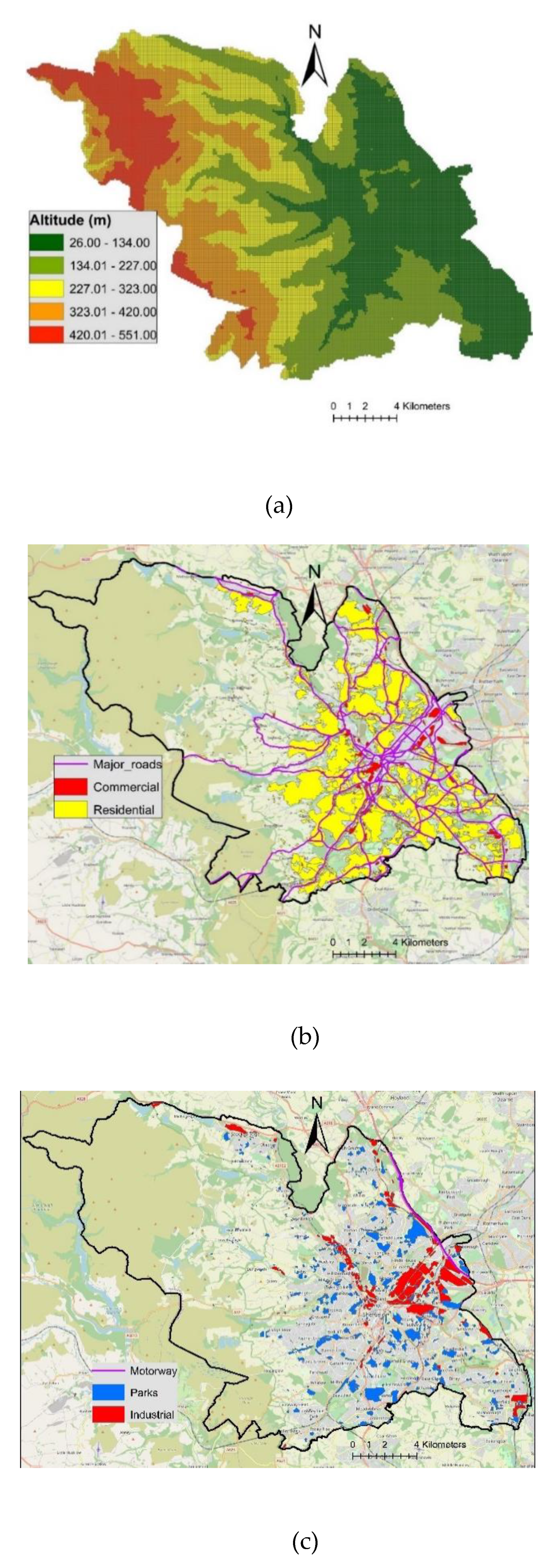
2.1. Predictor Variables and NO2 Monitoring Sites
- (a)
- Area (m2) of industrial land use, residential area, commercial area, parks and green area, and building area;
- (b)
- Length (m) of motorways, major roads, and minor roads;
- (c)
- Distance (m) to motorway, major road, minor road, building, industry, bus stop, parks, commercial area, and residential area;
- (d)
- Population (persons per km2), Altitude (m), number of bus stops, easting (m), northing (m), and street intersection.
2.2. LUR Model Development
- (1)
- Measurements of NO2 obtained from 188 DT;
- (2)
- Measurements of NO2 obtained from 40 LCS;
- (3)
- Combined NO2 measurements obtained from both LCS and DT (228).
- MLRM
- ii.
- GAM
2.3. Model Specification
2.4. Model Validation
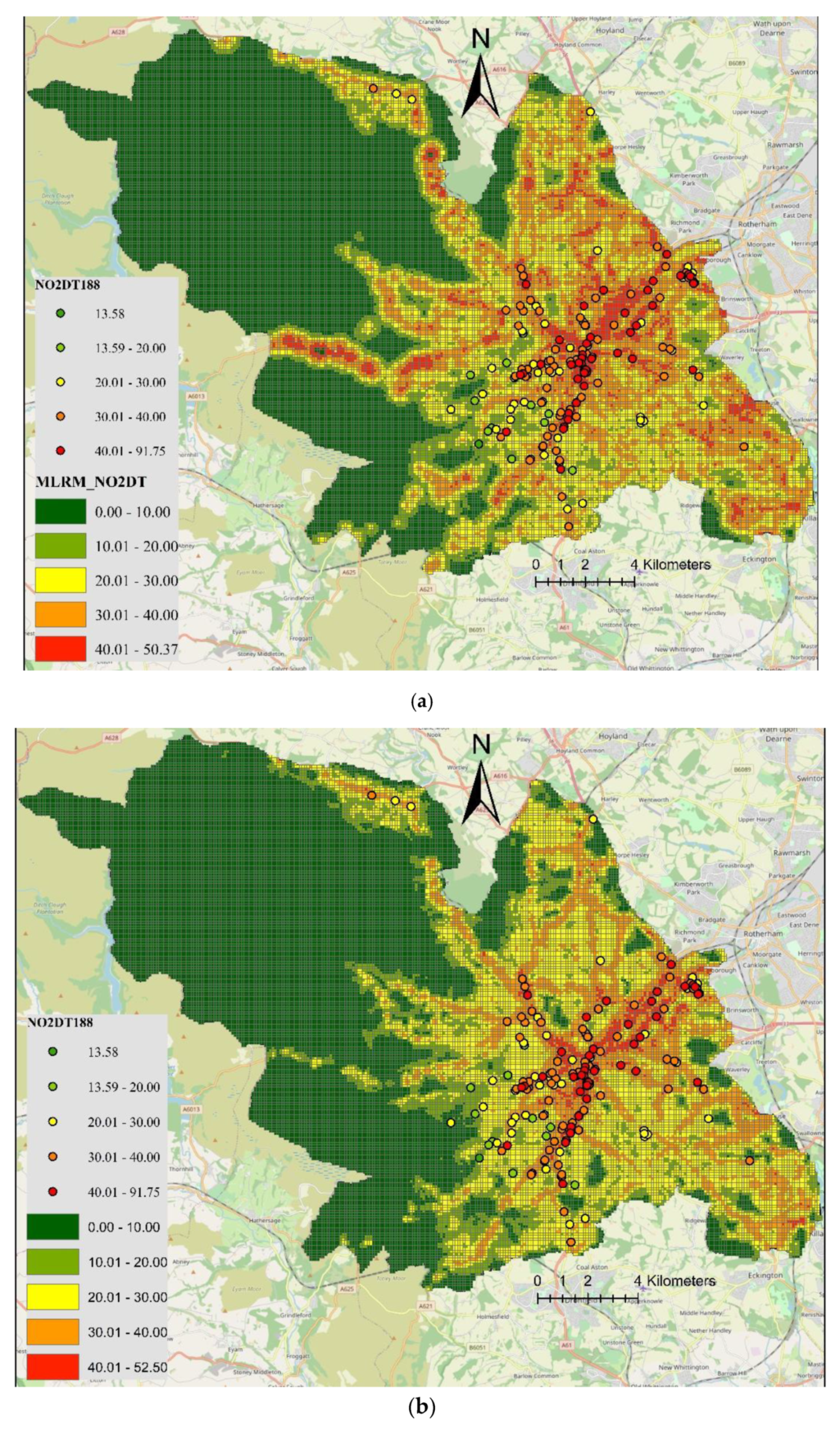
2.5. Mapping Modelled NO2 Concentration
2.6. Statistical Software
3. Results and Discussion
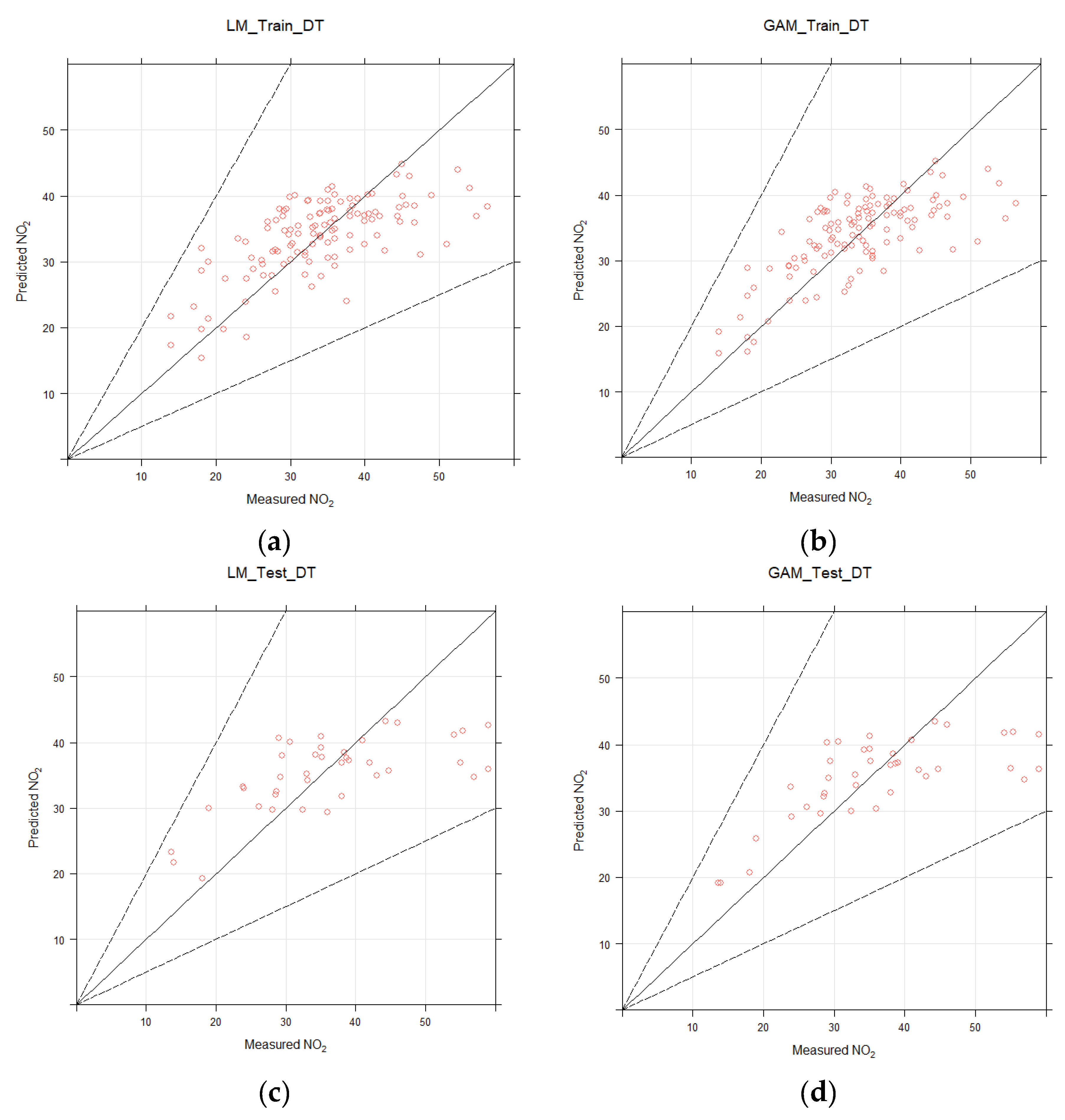
3.1. LUR Model Using NO2 Data from DT
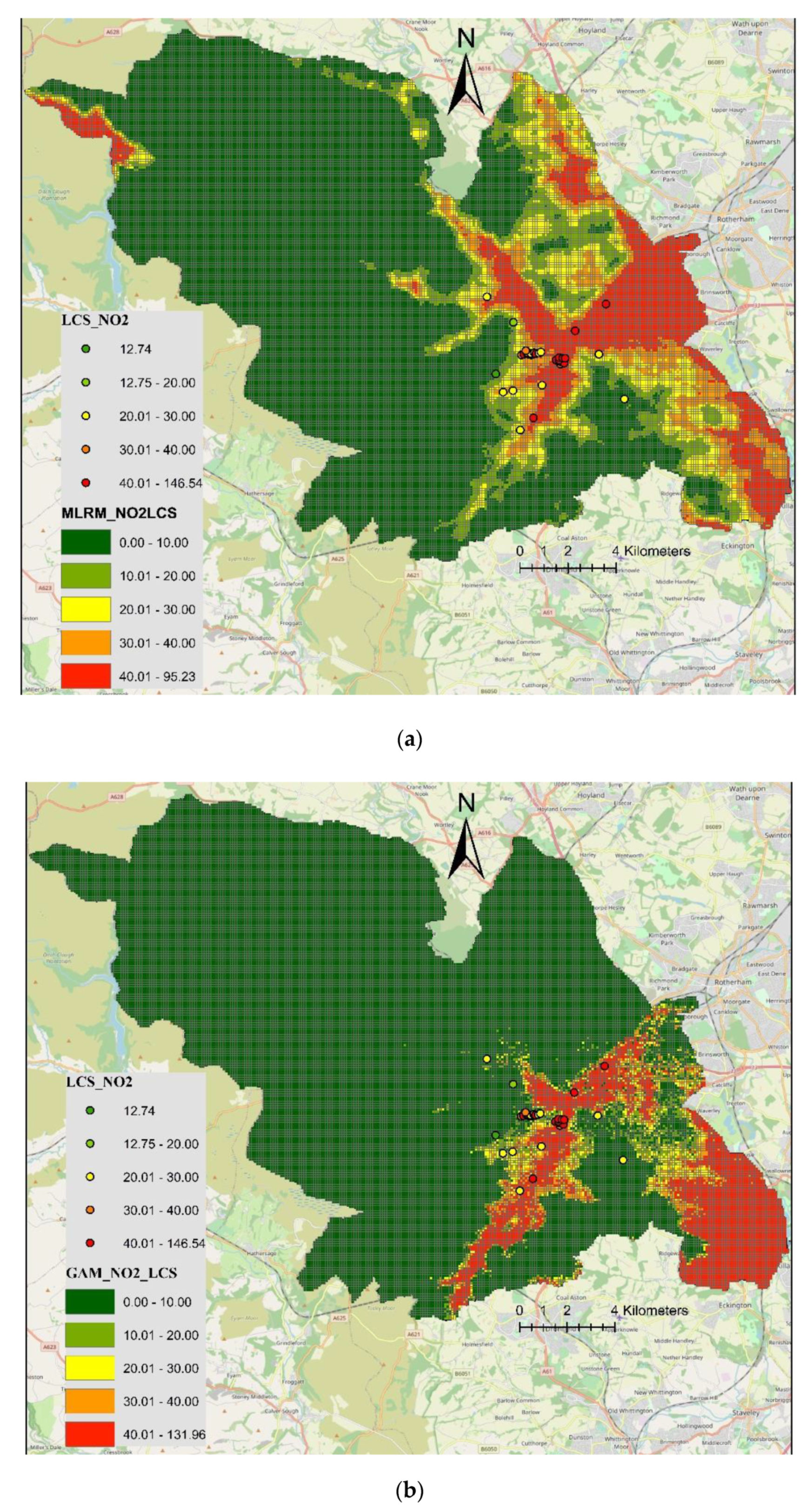
3.2. LUR Model Using NO2 Data from LCS
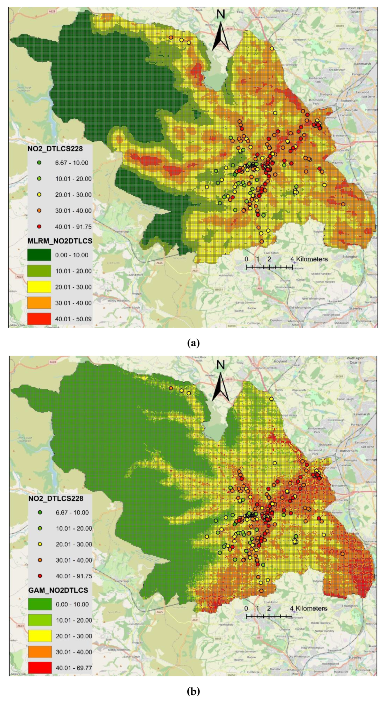
3.3. LUR Model Using NO2 Data from DT and LCS
4. Conclusions
Author Contributions
Funding
Acknowledgments
Conflicts of Interest
References
- Landrigan, P.J. Air pollution and health. Lancet Public Health 2016, 2, E4–E5. [Google Scholar] [CrossRef] [Green Version]
- WHO. Review of Evidence on Health Aspects of Air Pollution-REVIHAAP Project: Final Technical Report. World Health Organziation Regional Office for Europe, 2013. Available online: http://www.euro.who.int/en/health-topics/environment-and-health/airquality/publications/2013/review-of-evidence-on-health-aspects-of-air-pollutionrevihaap-project-final-technical-report (accessed on 12 February 2020).
- DEFRA. Improving Air Quality in the UK Tackling Nitrogen Dioxide in Our Towns and Cities, UK Overview Document. December 2015. Available online: https://www.gov.uk/government/uploads/system/uploads/attachment_data/file/486636/aq-plan-2015-overview-document.pdf (accessed on 9 April 2020).
- Hsu, S.; Mavrogianni, A.; Hamilton, I. Comparing spatial interpolation techniques of local urban temperature for heat-related health risk estimation in a subtropical city. Procedia Eng. 2017, 198, 354–365. [Google Scholar] [CrossRef]
- Briggs, D.J. The Role of Gis: Coping with Space (And Time) in Air Pollution Exposure Assessment. J. Toxicol. Environ. Health Part A 2005, 68, 1243–1261. [Google Scholar] [CrossRef] [PubMed]
- Schneider, P.; Castell, N.; Vogt, M.; Dauge, F.R.; Lahoz, W.A.; Bartonova, A. Mapping urban air quality in near real-time using observations from lowcost sensors and model information. Environ. Int. 2017, 106, 234–247. [Google Scholar] [CrossRef] [PubMed]
- Briggs, D.J.; De Hough, C.; Gulliver, J.; Wills, J.; Elliott, P.; Kingham, S.; Smallbone, K. A regression-based method for mapping traffic-related air pollution: Application and testing in four contrasting urban environments. Sci. Total Environ. 2000, 253, 151–167. [Google Scholar] [CrossRef]
- Hoek, G.; Beelen, R.; De Hoogh, K.; Vienneau, D.; Gulliver, J.; Fischer, P.; Briggs, D. A review of land-use regression models to assess spatial variation of outdoor air pollution. Atmos. Environ. 2008, 42, 7561–7578. [Google Scholar] [CrossRef]
- Briggs, D.J.; Collins, S.; Elliott, P.; Fischer, P.; Kingham, S.; Erik Lebret, K.P.; Van Reeuwijk, H.; Smallbone, K.; Van der Veen, A. Mapping urban air pollution using GIS: A regression-based approach. Int. J. Geogr. Inf. Sci. 1997, 11, 699–718. [Google Scholar] [CrossRef] [Green Version]
- Eeftens, M.; Beelen, R.; De Hoogh, K.; Bellander, T.; Cesaroni, G.; Cirach, M.; Declercq, C.; Dėdelė, A.; Dons, E.; De Nazelle, A.; et al. Development of land use regression models for PM2.5, PM2.5 absorbance, PM10 and PM coarse in 20 European Study areas; results of the ESCAPE project. Environ. Sci. Technol. 2012, 46, 11195–11205. [Google Scholar] [CrossRef]
- Lee, J.H.; Wu, C.F.; Hoek, G.; Hoogh, K.; Beelen, R.; Brunekreef, B.; Chan, C.-C. Land use regression models for estimating individual NOx and NO2 exposures in a metropolis with a high density of traffic roads and population. Sci. Total Environ. 2013, 472, 1163–1171. [Google Scholar] [CrossRef] [PubMed]
- Muttoo, S.; Ramsay, L.; Brunekreef, B.; Beelen, R.; Meliefste, K.; Naidoo, R.N. Land use regression modelling estimating nitrogen oxides exposure in industrial south Durban, South Africa. Sci. Total Environ. 2017, 610–611, 1439–1447. [Google Scholar] [CrossRef]
- Rahman, M.M.; Yeganeh, B.; Clifford, S.; Knibbs, L.D.; Morawska, L. Development of a land use regression model for daily NO2 and NOx concentrations in the Brisbane metropolitan area, Australia. Environ. Model. Softw. 2017, 95, 168–179. [Google Scholar] [CrossRef] [Green Version]
- Stedman, J.; Vincent, K.; Campbell, G.; Goodwin, J.; Downing, C. New high resolution maps of estimated background ambient NOx and NO2 concentrations in the U.K. Atmos. Environ. 1997, 31, 3591–3602. [Google Scholar] [CrossRef]
- Beelen, R.; Hoek, G.; Fischer, P.; Van den Brandt, P.A.; Brunekreef, B. Estimated long-term outdoor air pollution concentrations in a cohort study. Atmos. Environ. 2007, 41, 1343–1358. [Google Scholar] [CrossRef]
- Ryan, P.H.; LeMasters, G.K.; Biswas, P.; Levin, L.; Hu, S.; Lindsey, M.; Bernstein, D.I.; Lockey, J.; Villareal, M.; Hershey, G.K.K.; et al. A comparison of proximity and land use regression traffic exposure models and wheezing in infants. Environ. Health Perspect. 2007, 115, 278–284. [Google Scholar] [CrossRef] [Green Version]
- Ryan, P.H.; LeMasters, G.K. A review of land-use regressionmodels for characterizing intraurban air pollution exposure. Inhal. Toxicol. 2007, 19 (Suppl. 1), 127–133. [Google Scholar] [CrossRef] [Green Version]
- Gillespie, J.; Beverland, I.J.; Hamilton, S.; Padmanabhan, S. Development, Evaluation, and Comparison of Land Use Regression Modeling Methods to Estimate Residential Exposure to Nitrogen Dioxide in a Cohort Study. Environ. Sci. Technol. 2016, 50, 11085–11093. [Google Scholar] [CrossRef] [PubMed] [Green Version]
- Beelen, R.; Hoek, G.; Vienneau, D.; Eeftens, M.; Dimakopoulou, K.; Pedeli, X.; Tsai, M.Y. Development of NO2 and NOx land use regression models for estimating air pollution exposure in 36 study areas in Europe e-The ESCAPE project. Atmos. Environ. 2013, 72, 10–23. [Google Scholar] [CrossRef]
- Vienneau, D.; De Hoogh, K.; Beelen, R.; Fischer, P.; Hoek, G.; Briggs, D. Comparison of land-use regression models between Great Britain and the Netherlands. Atmos. Environ. 2010, 44, 688–696. [Google Scholar] [CrossRef]
- Munir, S.; Mayfield, M.; Coca, D.; Mihaylova, L.S.; Osammor, O. Analysis of air pollution in urban areas with Airviro dispersion—A Case Study in the City of Sheffield, United Kingdom. Atmosphere 2020, 11, 285. [Google Scholar] [CrossRef] [Green Version]
- Munir, S.; Mayfield, M.; Coca, D.; Jubb, S.A. Structuring an Integrated Air Quality Monitoring Nework in Large Urban Areas—Discussing the Purpose, Criteria and Deployment Strategy. Atmos. Environ. X 2019, 2, 100027. [Google Scholar]
- R Core Team. R: A Language and Environment for Statistical Computing; R Foundation for Statistical Computing: Vienna, Austria, 2019; Available online: https://www.R-project.org/.
- Wood, S.N.; Augustin, N.H. GAMs with integrated model selection using penalized regression splines and applications to environmental modelling. Ecol. Model. 2002, 157, 157–177. [Google Scholar] [CrossRef] [Green Version]
- Wood, S.N. Fast stable restricted maximum likelihood and marginal likelihood estimation of semiparametric generalized linear models. J. R. Stat. Soc. B 2011, 73, 3–36. [Google Scholar] [CrossRef] [Green Version]
- Wood, S.N. Generalized Additive Models: An Introduction with R 2006; Chapman and Hall: London, UK; CRC Press: Boca Raton, FL, USA, 2006. [Google Scholar]
- Hastie, T.J.; Tibshirani, R.J. Generalised Additive Models 1990; Chapman and Hall: London, UK, 1990. [Google Scholar]
- Venables, W.N.; Ripley, B.D. Modern Applied Statistics with S, 4th ed.; Springer: New York, NY, USA, 2002; ISBN 0-387-95457-0. [Google Scholar]
- Carslaw, D.C.; Ropkins, K. Openair—An R package for air quality data analysis. Environ. Model. Softw. 2012, 27–28, 52–61. [Google Scholar] [CrossRef]
- Korek, M.; Johansson, C.; Svensson, N.; Lind, T.; Beelen, R.; Hoek, G.; Pershagen, G.; Bellander, T. Can dispersion modeling of air pollution be improved by land-use regression? An example from Stockholm, Sweden. J. Expo. Sci. Environ. Epidemiol. 2017, 27, 575–581. [Google Scholar] [CrossRef] [Green Version]
- Ji, H.; Chen, S.; Zhang, Y.; Chen, H.; Guo, P.; Zhao, P. Comparison of air quality at different altitudes from multi-platform measurements in Beijing. Atmos. Chem. Phys. 2018, 18, 10645–10653. [Google Scholar] [CrossRef] [Green Version]
- Molter, A.; Lindley, S.; De Vocht, F.; Simpson, A.; Agius, R. Modelling air pollution for epidemiologic research—Part I: A novel approach combining land use regression and air dispersion. Sci. Total Environ. 2010, 408, 5862–5869. [Google Scholar] [CrossRef]


| Metrics | DT NO2 | LCS NO2 |
|---|---|---|
| Minimum | 13.58 | 12.74 |
| 1st Quartile (25th percentile) | 28.29 | 25.23 |
| Median | 33.77 | 33.19 |
| Mean | 34.23 | 41.23 |
| 3rd Quartile (75th percentile) | 40.00 | 45.28 |
| Maximum | 62.03 | 146.54 |
| Standard Deviation | 9.65 | 27.69 |
| Predictor Variable | Coefficient | p-Value |
|---|---|---|
| Intercept | 43.7025 | <2 × 10⁻¹⁶ *** |
| Building | 0.0020 | 0.075 + |
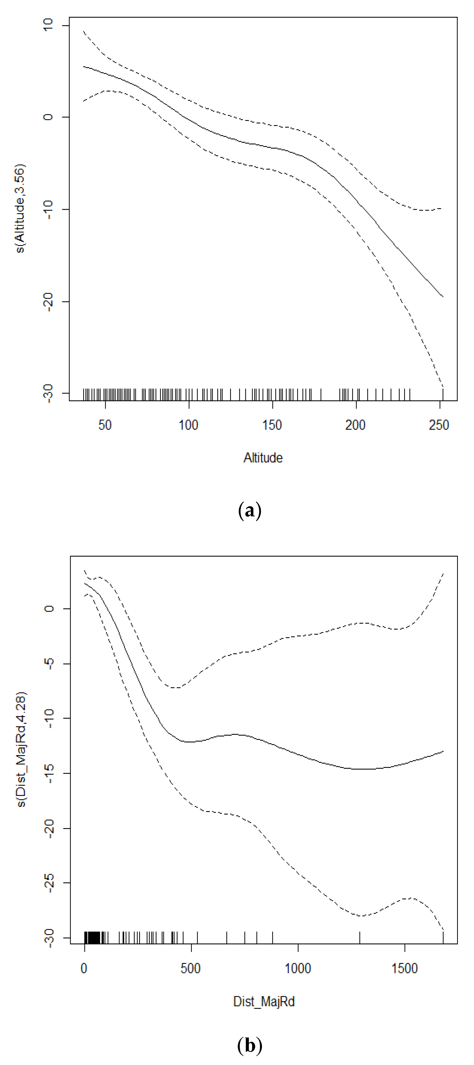
| Dist_MajorRd | −0.0114 | 0.001 ** |
| Dist_MinorRd | −0.0968 | 0.052 + |
| Residential | −0.0006 | 0.002 ** |
| Commercial | 0.0005 | 0.053 + |
| Altitude | −0.0543 | 0.000 *** |
| Dist_Bstop | −0.0308 | 0.026 * |
| Metrics | MLRM | GAM | ||
|---|---|---|---|---|
| FM | CV | FM | CV | |
| FAC2 | 1 | 1 | 1 | 1 |
| MB | 2 × 10⁻¹⁵ | −0.95 | 2 × 10⁻¹¹ | −1.17 |
| MGE | 4.98 | 6.89 | 4.80 | 6.55 |
| NMB | 2 × 10⁻¹⁷ | −0.03 | 2 × 10⁻¹² | −0.03 |
| NMGE | 0.15 | 0.19 | 0.14 | 0.18 |
| RMSE | 6.44 | 8.98 | 6.13 | 8.69 |
| r | 0.67 | 0.67 | 0.73 | 0.70 |
| Metrics | MLRM | GAM | ||
|---|---|---|---|---|
| FM | CV | FM | CV | |
| FAC2 | 0.97 | 1 | 1 | 0.90 |
| MB | 2 × 10⁻¹⁵ | −0.48 | 2 × 10⁻¹⁰ | −3.76 |
| MGE | 11.07 | 8.82 | 7.60 | 16.35 |
| NMB | 2 × 10⁻¹⁶ | −0.01 | 2 × 10⁻¹² | −0.10 |
| NMGE | 0.29 | 0.24 | 0.20 | 0.44 |
| RMSE | 19.31 | 12.56 | 10.40 | 22.21 |
| r | 0.55 | 0.78 | 0.89 | 0.56 |
| Metrics | MLRM | GAM | ||
|---|---|---|---|---|
| FM | CV | FM | CV | |
| FAC2 | 0.93 | 0.89 | 0.99 | 0.91 |
| MB | 2 × 10⁻¹⁵ | −2.28 | −4.01 | −2.03 |
| MGE | 7.31 | 9.32 | 6.49 | 9.21 |
| NMB | 2 × 10⁻¹⁶ | −0.09 | −1.28 | −0.07 |
| NMGE | 0.23 | 0.31 | 0.21 | 0.30 |
| RMSE | 9.47 | 12.33 | 8.62 | 12.22 |
| r | 0.60 | 0.52 | 0.69 | 0.53 |
© 2020 by the authors. Licensee MDPI, Basel, Switzerland. This article is an open access article distributed under the terms and conditions of the Creative Commons Attribution (CC BY) license (http://creativecommons.org/licenses/by/4.0/).
Share and Cite
Munir, S.; Mayfield, M.; Coca, D.; Mihaylova, L.S. A Nonlinear Land Use Regression Approach for Modelling NO2 Concentrations in Urban Areas—Using Data from Low-Cost Sensors and Diffusion Tubes. Atmosphere 2020, 11, 736. https://0-doi-org.brum.beds.ac.uk/10.3390/atmos11070736
Munir S, Mayfield M, Coca D, Mihaylova LS. A Nonlinear Land Use Regression Approach for Modelling NO2 Concentrations in Urban Areas—Using Data from Low-Cost Sensors and Diffusion Tubes. Atmosphere. 2020; 11(7):736. https://0-doi-org.brum.beds.ac.uk/10.3390/atmos11070736
Chicago/Turabian StyleMunir, Said, Martin Mayfield, Daniel Coca, and Lyudmila S Mihaylova. 2020. "A Nonlinear Land Use Regression Approach for Modelling NO2 Concentrations in Urban Areas—Using Data from Low-Cost Sensors and Diffusion Tubes" Atmosphere 11, no. 7: 736. https://0-doi-org.brum.beds.ac.uk/10.3390/atmos11070736