Variations in Ozone Concentration over the Mid-Latitude Region Revealed by Ozonesonde Observations in Pohang, South Korea


Abstract
:1. Introduction
2. Materials and Methods
2.1. Data and Period
2.2. Electrochemical Concentration Cells Ozonesonde
2.3. Data Selection
2.4. Altitude Classification for Analysis
3. Results
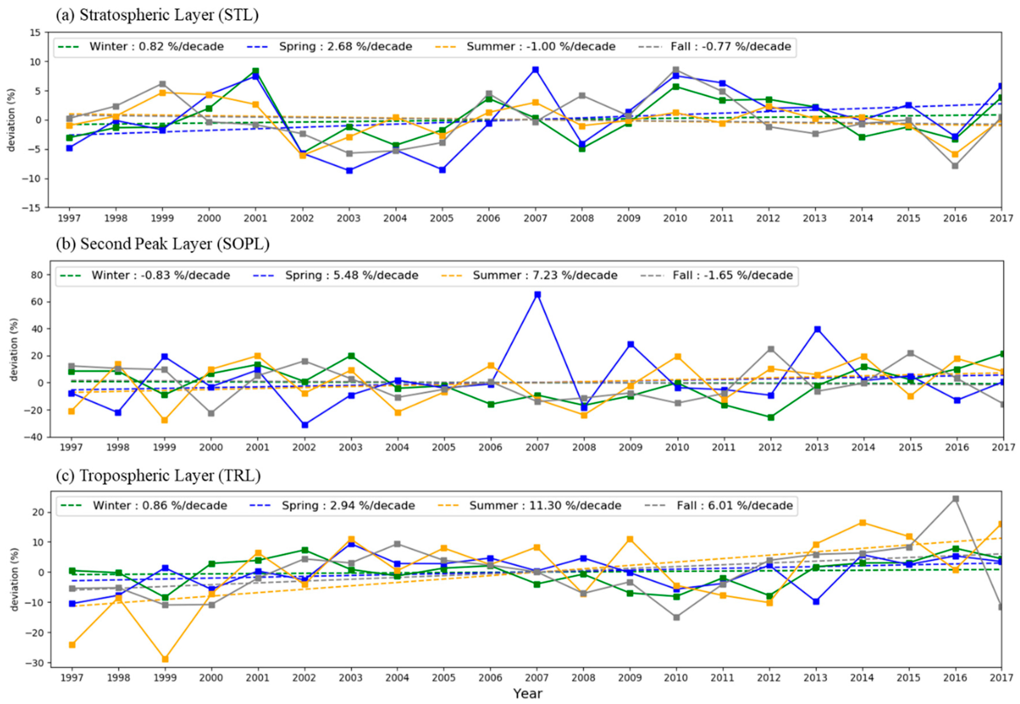
3.1. Trend Analysis
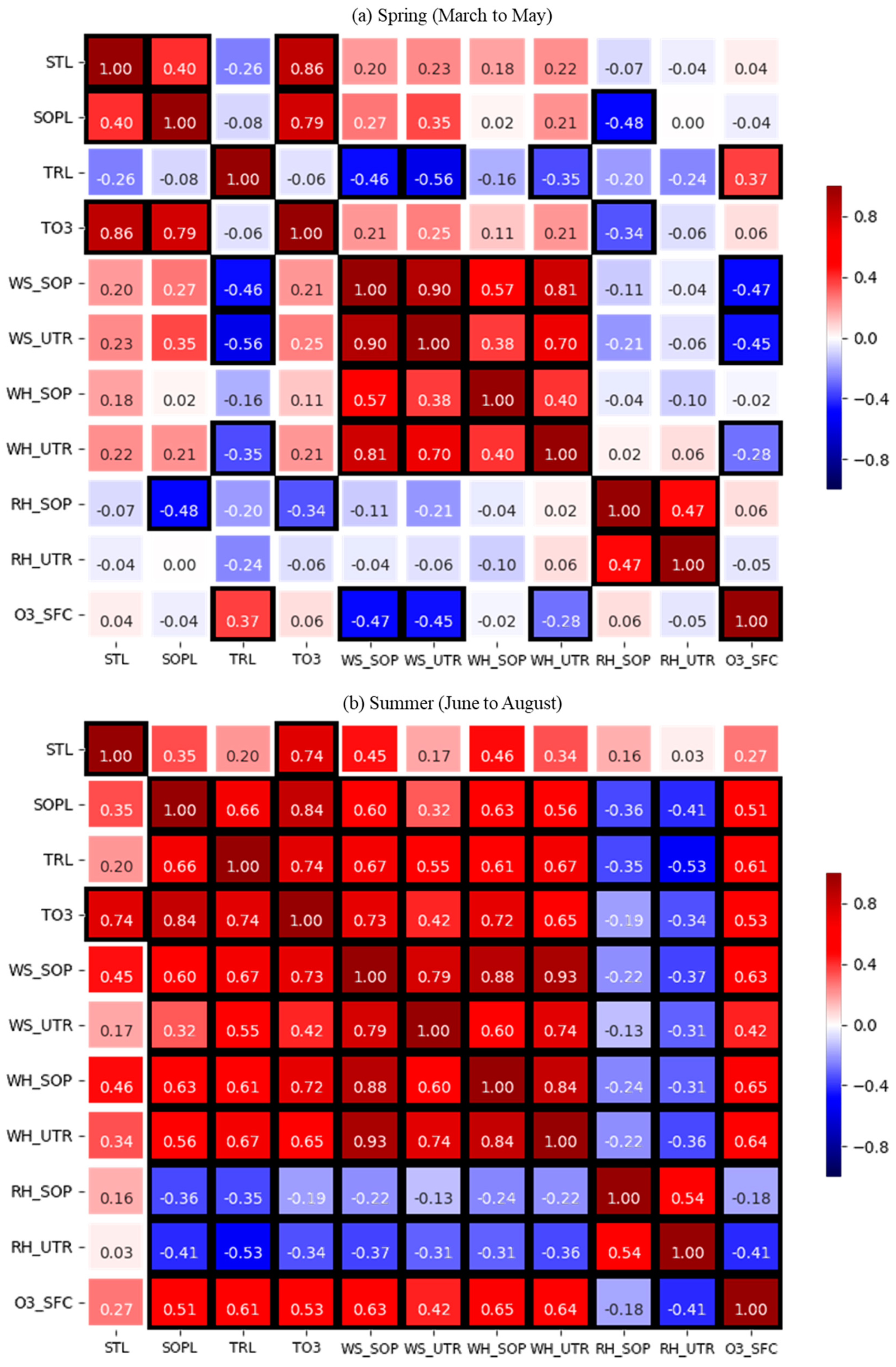
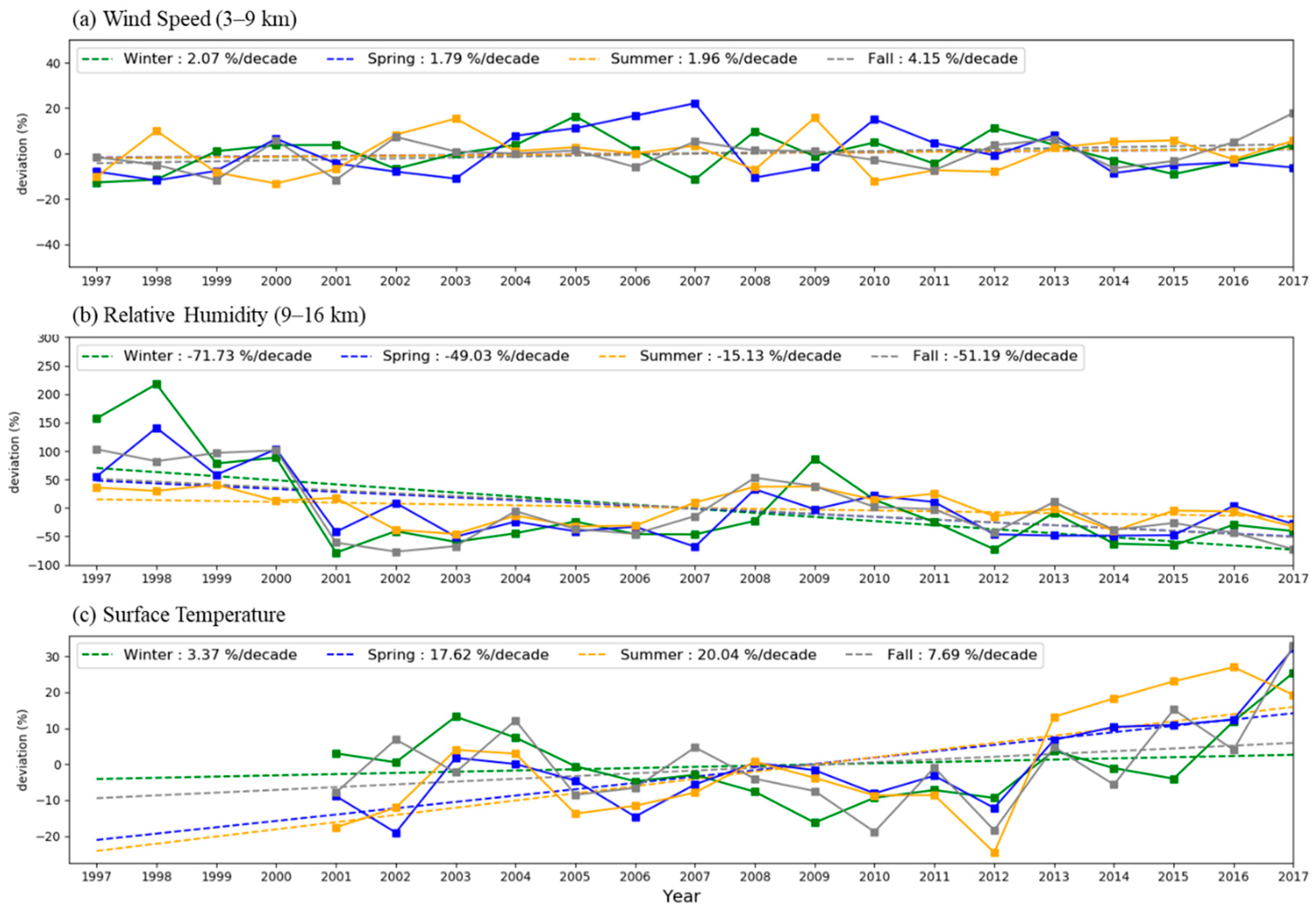
3.2. Influence Components Analysis
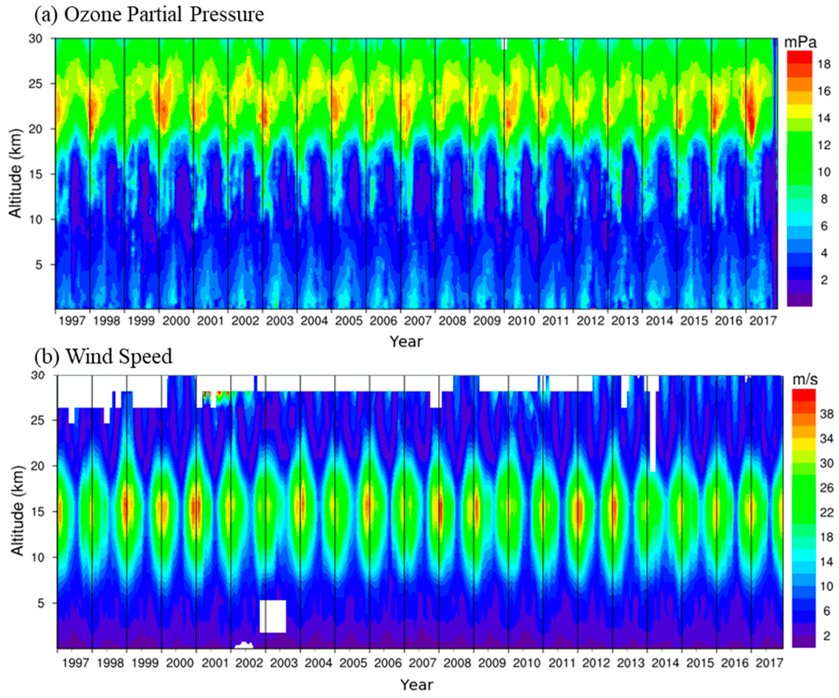
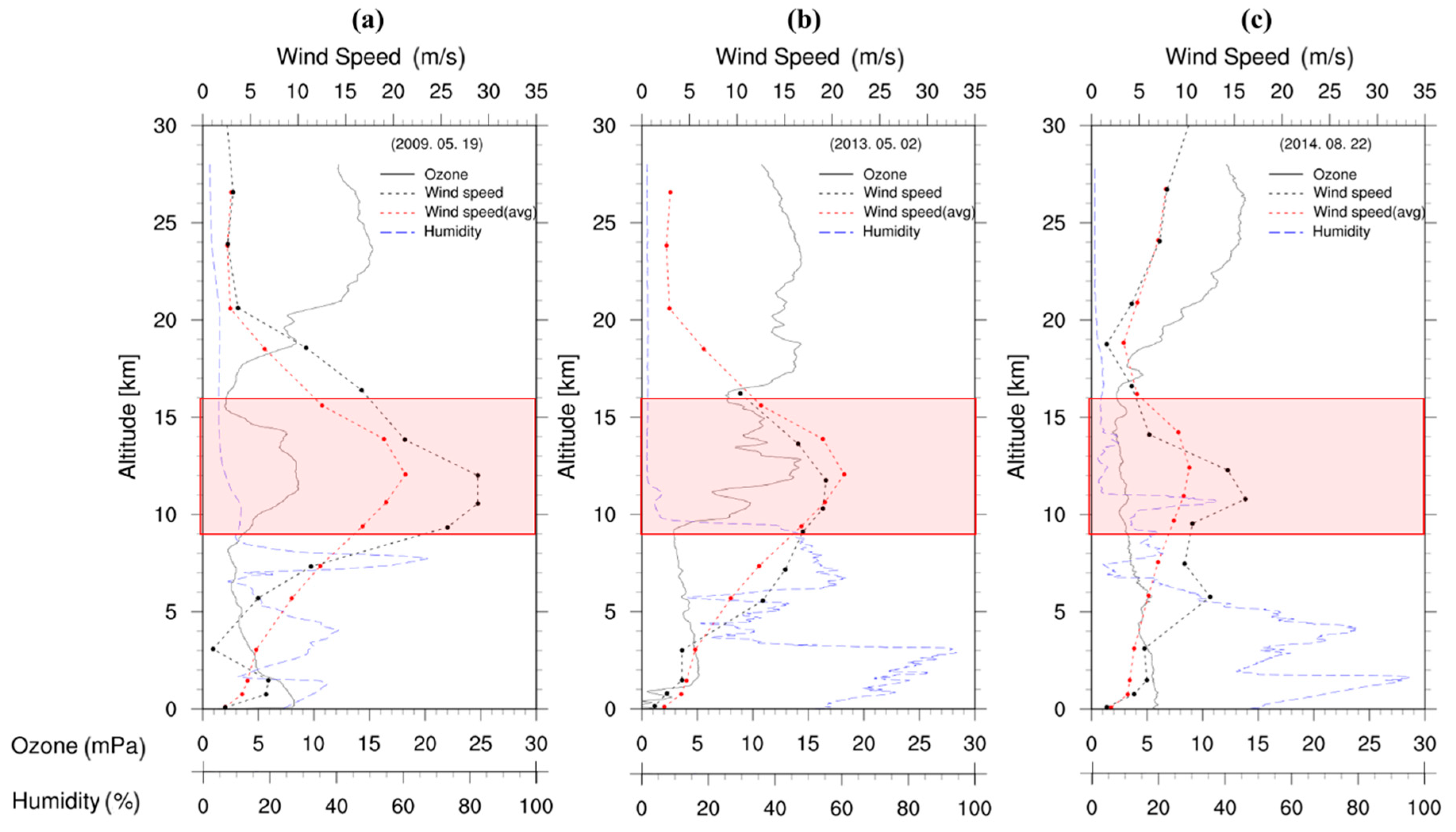
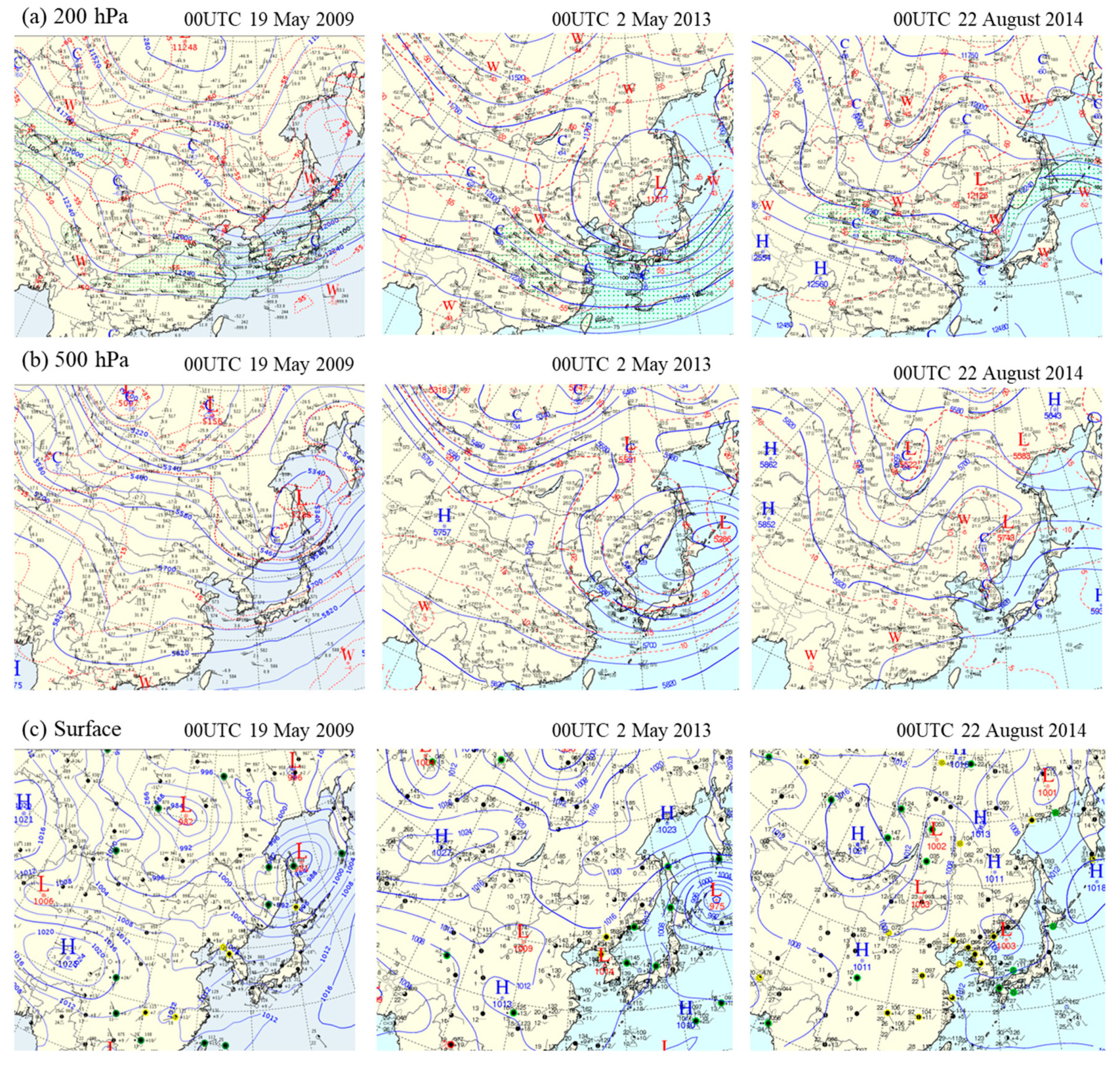
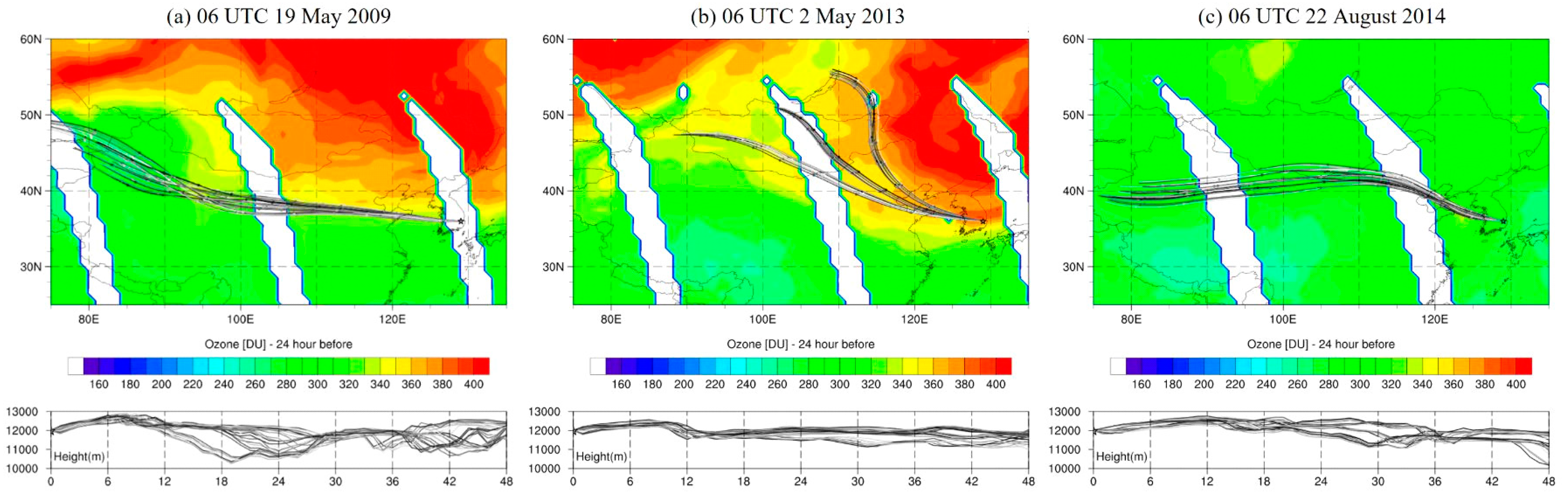
3.3. Characteristics of the Second Ozone Peak Generation
4. Conclusions
Author Contributions
Funding
Acknowledgments
Conflicts of Interest
References
- Stocker, T.F.; Qin, D.; Plattner, G.K.; Tignor, M.; Allen, S.K.; Boschung, J.; Nauels, A.; Xia, Y.; Bex, V.; Midgley, P.M. Climate Change 2013: The Physical Science Basis, Contribution of Working Group I to the Fifth Assessment Report of the Intergovernmental Panel on Climate Change; Cambridge University Press: Cambridge, UK; New York, NY, USA, 2013; p. 1535. [Google Scholar]
- World Meteorological Organization. Scientific Assessment of Ozone Depletion: 2014, Global Ozone Research and Monitoring Project—Report No. 55; World Meteorological Organization: Geneva, Switzerland, 2014. [Google Scholar]
- Staehelin, J.; Harris, N.R.P.; Appenzeller, C.; Eberhard, J. Ozone trends: A review. Rev. Geophys. 2001, 39, 231–290. [Google Scholar] [CrossRef] [Green Version]
- Kim, J.; Cho, H.K.; Lee, Y.G.; Oh, S.N.; Baek, S.-K. Updated trends of stratospheric ozone over Seoul. J. Atmos. 2005, 15, 101–118. [Google Scholar]
- Chehade, W.; Weber, M.; Burrows, J.P. Total ozone trends and variability during 1979–2012 from merged data sets of various satellites. Atmos. Chem. Phys. 2014, 14, 7059–7074. [Google Scholar] [CrossRef] [Green Version]
- Pawson, S.; Steinbrecht, W.; Charlton-Perez, A.J.; Fujiwara, M.; Karpechko, A.Y.; Petropavlovskikh, I.; Urban, J.; Weber, M. Update on Global Ozone: Past, Present, and Future. Scientific Assessment of Ozone Depletion, World Meteorological Organization, Global Ozone Research and Monitoring Project—Report No. 55; World Meteorological Organization: Geneva, Switzerland, 2014; Chapter 2. [Google Scholar]
- Shepherd, T.G.; Plummer, D.A.; Scinocca, J.F.; Hegglin, M.I.; Fioletov, V.; Reader, M.C.; Remsberg, E.; Von Clarmann, T.; Wang, H.J. Reconciliation of halogen-induced ozone loss with the total-column ozone record. Nat. Geosci. 2014, 7, 443–449. [Google Scholar] [CrossRef] [Green Version]
- Zvyagintsev, A.M.; Vargin, P.N.; Peshin, S. Total ozone variations and trends during the period 1979–2014. Atmos. Ocean. Opt. 2015, 28, 575–584. [Google Scholar] [CrossRef]
- Solomon, S.; Ivy, D.J.; Kinnison, D.; Mills, M.J.; Neely, R.; Schmidt, A. Emergence of healing in the Antarctic ozone layer. Science 2016, 353, 269–274. [Google Scholar] [CrossRef] [Green Version]
- Chipperfield, M.P.; Bekki, S.; Dhomse, S.S.; Harris, N.R.P.; Hassler, B.; Hossaini, R.; Steinbrecht, W.; Thiéblemont, R.; Weber, M. Detecting recovery of the stratospheric ozone layer. Nature 2017, 549, 211–218. [Google Scholar] [CrossRef] [Green Version]
- Rigby, M.; Park, S.; Saito, T.; Western, L.M.; Redington, A.L.; Fang, X.; Henne, S.; Manning, A.J.; Prinn, R.G.; Dutton, G.; et al. Increase in CFC-11 emissions from eastern China based on atmospheric observations. Nature 2019, 569, 546–550. [Google Scholar] [CrossRef]
- Dameris, M.; Jöckel, P.; Nützel, M. Possible implications of enhanced chlorofluorocarbon-11 concentrations on ozone. Atmos. Chem. Phys. Discuss. 2019, 19, 13759–13771. [Google Scholar] [CrossRef] [Green Version]
- Montzka, S.A.; Dutton, G.; Yu, P.; Ray, E.; Portmann, R.W.; Daniel, J.S.; Kuijpers, L.; Hall, B.D.; Mondeel, D.; Siso, C.; et al. An unexpected and persistent increase in global emissions of ozone-depleting CFC-11. Nature 2018, 557, 413–417. [Google Scholar] [CrossRef]
- Park, S.S.; Kim, J.; Cho, H.K.; Lee, H.; Lee, Y.J.; Miyagawa, K. Sudden increase in the total ozone density due to secondary ozone peaks and its effect on total ozone trends over Korea. Atmos. Environ. 2012, 47, 226–235. [Google Scholar] [CrossRef]
- Collins, W.J.; Derwent, R.G.; Garnier, B.; Johnson, C.E.; Sanderson, M.G.; Stevenson, D. Effect of stratosphere-troposphere exchange on the future tropospheric ozone trend. J. Geophys. Res. Space Phys. 2003, 108. [Google Scholar] [CrossRef] [Green Version]
- Hwang, S.-H.; Kim, J.; Cho, G.-R. Observation of secondary ozone peaks near the tropopause over the Korean peninsula associated with stratosphere-troposphere exchange. J. Geophys. Res. Space Phys. 2007, 112. [Google Scholar] [CrossRef] [Green Version]
- Hegglin, M.I.; Shepherd, T.G. Large climate-induced changes in ultraviolet index and stratosphere-to-troposphere ozone flux. Nat. Geosci. 2009, 2, 687–691. [Google Scholar] [CrossRef]
- Butchart, N. The Brewer-Dobson circulation. Rev. Geophys. 2014, 52, 157–184. [Google Scholar] [CrossRef]
- Hess, P.; Kinnison, D.; Tang, Q. Ensemble simulations of the role of the stratosphere in the attribution of northern extratropical tropospheric ozone variability. Atmos. Chem. Phys. Discuss. 2015, 15, 2341–2365. [Google Scholar] [CrossRef] [Green Version]
- Hocking, W.K.; Carey-Smith, T.; Tarasick, D.W.; Argall, P.S.; Strong, K.; Rochon, Y.; Zawadzki, I.; Taylor, P.A. Detection of stratospheric ozone intrusions by wind profiler radars. Nature 2007, 450, 281–284. [Google Scholar] [CrossRef]
- Stevenson, D.; Dentener, F.J.; Schultz, M.; Ellingsen, K.; Van Noije, T.P.C.; Wild, O.; Zeng, G.; Amann, M.; Atherton, C.S.; Bell, N.; et al. Multimodel ensemble simulations of present-day and near-future tropospheric ozone. J. Geophys. Res. Space Phys. 2006, 11. [Google Scholar] [CrossRef] [Green Version]
- Hofmann, C.; Kerkweg, A.; Hoor, P.; Jöckel, P. Stratosphere-troposphere exchange in the vicinity of a tropopause fold. Atmos. Chem. Phys. Discuss. 2016, 1–26. [Google Scholar] [CrossRef] [Green Version]
- Shin, H.J.; Park, J.H.; Park, J.S.; Song, I.H.; Park, S.M.; Roh, S.A.; Son, J.S.; Hong, Y.D. The Long Term Trends of Tropospheric Ozone in Major Regions in Korea. Asian J. Atmos. Environ. 2017, 11, 235–253. [Google Scholar] [CrossRef] [Green Version]
- Brewer, A.W.; Milford, J.R. The Oxford-Kew ozone sonde. Proc. R. Soc. Lond. Ser. A Math. Phys. Sci. 1960, 256, 470–495. [Google Scholar] [CrossRef]
- Komhyr, W.D. Electrochemical concentration cells for gas analysis. Ann. Geophys. 1969, 25, 203–210. [Google Scholar]
- Kobayashi, J.; Toyama, Y. On various methods of measuring the vertical distribution of atmospheric ozone (III) carbon-iodine type chemical ozonesonde. Pap. Meteorol. Geophys. 1966, 17, 113–126. [Google Scholar] [CrossRef] [Green Version]
- Smit, H.G.; Straeter, W.; Johnson, B.J.; Oltmans, S.J.; Davies, J.; Tarasick, D.W.; Hoegger, B.; Stubi, R.; Schmidlin, F.J.; Northam, T.; et al. Assessment of the performance of ECC-ozonesondes under quasi-flight conditions in the environmental simulation chamber: Insights from the Juelich Ozone Sonde Intercomparison Experiment (JOSIE). J. Geophys. Res. Space Phys. 2007, 112. [Google Scholar] [CrossRef]
- Komhyr, W.D.; Harris, T.B. Development of an ECC-Ozonesonde; NOAA Technical report ERL, 200, APCL 18; NOAA: Boulder, CO, USA, 1971; p. 54. [Google Scholar]
- Kivi, R.; Kyrö, E.; Turunen, T.; Harris, N.R.P.; Von Der Gathen, P.; Rex, M.; Andersen, S.; Wohltmann, I. Ozonesonde observations in the Arctic during 1989–2003: Ozone variability and trends in the lower stratosphere and free troposphere. J. Geophys. Res. Space Phys. 2007, 112. [Google Scholar] [CrossRef] [Green Version]
- Deshler, T.; Mercer, J.L.; Smit, H.G.; Stubi, R.; Levrat, G.; Johnson, B.J.; Oltmans, S.J.; Kivi, R.; Thompson, A.M.; Witte, J.; et al. Atmospheric comparison of electrochemical cell ozonesondes from different manufacturers, and with different cathode solution strengths: The Balloon Experiment on Standards for Ozonesondes. J. Geophys. Res. Space Phys. 2008, 113. [Google Scholar] [CrossRef]
- Liu, G.; Tarasick, D.W.; Fioletov, V.; Sioris, C.E.; Rochon, Y.J. Ozone correlation lengths and measurement uncertainties from analysis of historical ozonesonde data in North America and Europe. J. Geophys. Res. Space Phys. 2009, 114. [Google Scholar] [CrossRef]
- Morris, G.A.; Labow, G.; Akimoto, H.; Takigawa, M.; Fujiwara, M.; Hasebe, F.; Hirokawa, J.; Koide, T. On the use of the correction factor with Japanese ozonesonde data. Atmos. Chem. Phys. Discuss. 2013, 13, 1243–1260. [Google Scholar] [CrossRef] [Green Version]
- Smit, H.G.J. Chemistry of the Atmosphere: Observations for Chemistry (In Situ): Ozone Sondes. Encyclopedia of Atmospheric Sciences, 2nd ed.; Academic Press: New York, NY, USA, 2015; pp. 372–378. [Google Scholar]
- Smit, H.G.J.; Kley, D. JOSIE: The 1996 WMO International Intercomparison of Ozonesondes under Quasi-Flight Conditions in the Environmental Chamber at Jülich; WMO/IGAC-Report, WMO Global Atmosphere Watch report series, No. 130 (Technical Document No. 926); World Meteorological Organization: Geneva, Switzerland, 1996. [Google Scholar]
- McPeters, R.D.; Labow, G.J.; Johnson, B.J. A satellite-derived ozone climatology for balloonsonde estimation of total column ozone. J. Geophys. Res. Space Phys. 1997, 102, 8875–8885. [Google Scholar] [CrossRef]
- Bhartia, P.K. OMI/Aura TOMS-Like Ozone, Aerosol Index, Cloud Radiance Fraction L3 1 Day 1 Degree x 1 Degree V3, NASA Goddard Space Flight Center, Goddard Earth Sciences Data and Information Services Center (GES DISC). Available online: https://0-doi-org.brum.beds.ac.uk/10.5067/Aura/OMI/DATA3001 (accessed on 8 July 2019).
- Dhomse, S.S.; Feng, W.; Montzka, S.A.; Hossaini, R.; Keeble, J.; Pyle, J.A.; Daniel, J.S.; Chipperfield, M.P. Delay in recovery of the Antarctic ozone hole from unexpected CFC-11 emissions. Nat. Commun. 2019, 10, 1–12. [Google Scholar] [CrossRef] [Green Version]
- Revell, L.; Tummon, F.; Salawitch, R.J.; Stenke, A.; Peter, T. The changing ozone depletion potential of N2O in a future climate. Geophys. Res. Lett. 2015, 42. [Google Scholar] [CrossRef] [Green Version]
- Itahashi, S.; Uno, I.; Kim, S. Seasonal source contributions of tropospheric ozone over East Asia based on CMAQeHDDM. Atmos. Environ. 2013, 70, 204–217. [Google Scholar] [CrossRef]
- Lemoine, R. Secondary maxima in ozone profiles. Atmos. Chem. Phys. Discuss. 2004, 4, 1085–1096. [Google Scholar] [CrossRef] [Green Version]
- Kim, J.; Lee, H.J.; Lee, S.H. The Characteristics of Tropospheric Ozone Seasonality Observed from Ozone Soundings at Pohang, Korea. Environ. Monit. Assess. 2006, 118, 1–12. [Google Scholar] [CrossRef] [PubMed]
- Mohanakumar, K. Stratosphere Troposphere Interactions; Springer Science and Business Media LLC: Dordrecht, The Netherlands, 2008; pp. 331–355. [Google Scholar]
- Browning, K.A.; Reynolds, R. Diagnostic study of a narrow cold frontal rainband and severe winds associated with a stratospheric intrusion. Q. J. R. Meteorol. Soc. 1994, 120, 235–257. [Google Scholar] [CrossRef]
- Goering, M.A.; Gallus, W.A.; Olsen, M.A.; Stanford, J.L. Role of stratospheric air in a severe weather event: Analysis of potential vorticity and total ozone. J. Geophys. Res. Space Phys. 2001, 106, 813–823. [Google Scholar] [CrossRef]
- Stohl, A.; Bonasoni, P.; Collins, W.J.; Feichter, J.; Forster, C.; Gerasopoulos, E.; Gaggeler, H.; Kentarchos, T.; Kromp-Kolb, H.; Meloen, J.; et al. Stratosphere-troposphere exchange: A review, and what we have learned from STACCATO. J. Geophys. Res. Space Phys. 2003, 108, 8516. [Google Scholar] [CrossRef]
- Corsmeier, U.; Kalthoff, N.; Kolle, O.; Kotzian, M.; Fiedler, F. Ozone concentration jump in the stable nocturnal boundary layer during a LLJ-event. Atmos. Environ. 1997, 31, 1977–1989. [Google Scholar] [CrossRef]
- Minoura, H. Some characteristics of surface ozone concentration observed in an urban atmosphere. Atmos. Res. 1999, 51, 153–169. [Google Scholar] [CrossRef]
- Pugliese, S.C.; Murphy, J.G.; Geddes, J.; Wang, J.M. The impacts of precursor reduction and meteorology on ground-level ozone in the Greater Toronto Area. Atmos. Chem. Phys. Discuss. 2014, 14, 8197–8207. [Google Scholar] [CrossRef] [Green Version]
- Kang, Y.-H.; Kim, Y.-K.; Hwang, M.-K.; Jeong, J.-H.; Kim, H.; Kang, M.-S. Spatial-temporal variations in surface ozone concentrations in Busan metropolitan area. J. Environ. Sci. Int. 2019, 28, 169–182. [Google Scholar] [CrossRef]
- Donald, C. Meteorology Today: An Introduction to Weather, Climate, and the Environment; Cengage Learning: Boston, MA, USA, 2012; pp. 231–234. [Google Scholar]
- Kim, Y.K.; Moon, Y.S.; Song, S.K. Stratsophere-troposphere Exchange of Ozone Associated with the Upper Level Jet Stream. Asia Pac. J. Atmos. Sci. 2002, 38, 531–545. [Google Scholar]
- Yang, H.; Chen, G.; Tang, Q.; Hess, P. Quantifying isentropic stratosphere-troposphere exchange of ozone. J. Geophys. Res. Atmos. 2016, 121, 3372–3387. [Google Scholar] [CrossRef] [Green Version]
- Davies, T.; Schuepbach, E. Episodes of high ozone concentrations at the earth’s surface resulting from transport down from the upper troposphere/lower stratosphere: A review and case studies. Atmos. Environ. 1994, 28, 53–68. [Google Scholar] [CrossRef]
- Jeong, J.I.; Park, R.J.; Youn, D. Effects of Siberian forest fires on air quality in East Asia during May 2003 and its climate implication. Atmos. Environ. 2008, 42, 8910–8922. [Google Scholar] [CrossRef]


© 2020 by the authors. Licensee MDPI, Basel, Switzerland. This article is an open access article distributed under the terms and conditions of the Creative Commons Attribution (CC BY) license (http://creativecommons.org/licenses/by/4.0/).
Share and Cite
Shin, D.; Song, S.; Ryoo, S.-B.; Lee, S.-S. Variations in Ozone Concentration over the Mid-Latitude Region Revealed by Ozonesonde Observations in Pohang, South Korea. Atmosphere 2020, 11, 746. https://0-doi-org.brum.beds.ac.uk/10.3390/atmos11070746
Shin D, Song S, Ryoo S-B, Lee S-S. Variations in Ozone Concentration over the Mid-Latitude Region Revealed by Ozonesonde Observations in Pohang, South Korea. Atmosphere. 2020; 11(7):746. https://0-doi-org.brum.beds.ac.uk/10.3390/atmos11070746
Chicago/Turabian StyleShin, Daegeun, Seungjoo Song, Sang-Boom Ryoo, and Sang-Sam Lee. 2020. "Variations in Ozone Concentration over the Mid-Latitude Region Revealed by Ozonesonde Observations in Pohang, South Korea" Atmosphere 11, no. 7: 746. https://0-doi-org.brum.beds.ac.uk/10.3390/atmos11070746