Monitoring Dust Events Using Doppler Lidar and Ceilometer in Iceland

Abstract

Ground-based lidars and ceilometers are widely used for dust and volcanic ash observation around the world. This is particularly interesting in Iceland where high-altitude dust events occur frequently during strong wind conditions and volcanic eruptions. To explore the possible application of such technologies in Iceland for monitoring dust events, we used a combination of Doppler wind lidars with depolarization channels, ceilometers, and other instruments, to monitor two dust events that occurred in Iceland during summer 2019. We applied a verified ceilometer data processing procedure with customized local corrections and developed a new procedure to process Doppler lidar data for aerosols measurements. Both lidar and ceilometer observations can be used to detect the dust layer and reveal the temporal and vertical distribution of dust aerosols in Iceland. The depolarization ratio measurements indicate that the weather conditions, e.g., relative humidity, could have a significant impact on lidar measurements. We conclude that using Doppler wind lidar and ceilometer measurements to monitor volcanic and sedimentary aerosols is possible and may be used to provide important information to the scientific community.

1. Introduction

A lidar (light detection and ranging) system is an active remote sensing technology, which is used in different sectors, from auto-driven cars’ sensor [1] to civil engineering structure monitoring [2]. It is also used in meteorology, mainly focused on wind detection [3,4,5,6] and aerosol and cloud detection [7,8], depending on the type of lidar.

The lidar is emitting a laser beam and receives the backscattered signals, which could be airborne aerosols, cloud droplets, or other particles in the atmosphere. In principle, we can retrieve the properties of the scatterers from the lidar backscatter signals. The most commonly used variable is the backscatter coefficient, which is available for elastic-backscatter lidars. With Raman lidars or high spectral resolution lidars (HSRL), the extinction coefficient profiles, which are related to the absorbed lidar signals, can be measured directly, and the lidar ratio can be calculated based on the backscatter and extinction coefficient [7]. With a depolarization channel, lidars can measure the depolarization ratio and estimate the particles’ shape [9]. A combination of the lidar ratio and the depolarization ratio is commonly used for aerosol classification and volcanic ash discrimination [8,10].

A Doppler wind lidar is mainly used for wind measurements, including wind field/profiles retrieval [3], low-level jet detection [11], and atmospheric turbulence detection [12]. Lidar systems have been used widely for enhancing aviation safety around the world [13,14,15]. In Iceland, two Doppler wind lidars have been deployed for volcanic ash detection.

Besides Doppler lidar, another remote sensing instrument used in Iceland for aerosol detection is the ceilometer, i.e., eye-safe single-wavelength backscatter lidar. The ceilometer is designed for cloud base detection but also used for aerosol observations, such as dust layer [16] and volcanic ash detection [17]. A significant advantage of ceilometers is that they can run unattended and continuously, resulting in unique data to monitor aerosol distributions. Moreover, as they are inexpensive compared to other lidars, networks can be installed.

Iceland comprises a large sandy desert in the central plateau, covering 22,000 km² or almost 20% of the country [18]. The subarctic weather in Iceland is characterized by strong wind events [19] due to the frequent passing of low-pressure systems and associated weather fronts. This results in wind erosion leading to frequent dust storms. Furthermore, volcanic eruptions occur on average every three to five years [20]. Dust from a desert as well as volcanic ash from eruptions could have a significant impact locally and globally on radiation balance, economics, and human health [21,22,23,24,25,26]. According to observations at 30 Icelandic weather stations between 1949 and 2010, on average, there are 34 days of dust events annually. If the re-suspension of volcanic materials is considered as well, the number increases to 135 days [27]. In 2010, the explosive eruption of Eyjafjallajokull, and the subsequent ash cloud disrupted air traffic generating great economic loss [28,29]. Accordingly, an adequate method to monitor the ash dispersion continuously could improve aviation safety significantly.

The volcanic ash can be transported all over Europe and has been studied with satellite [30], airborne [31], and ground-based remote sensing technologies [32,33,34], including lidar, in different countries other than Iceland. However, aerosol monitoring in Iceland has only been investigated in a few studies. Prospero et al. [35] assessed Icelandic dust over the North Atlantic using aerosol concentration measurements in South Iceland. Dagsson-Waldhauserova et al. [36] measured the vertical profiles of aerosols in Iceland using airborne measurements. But the ground-based remote sensing measurements of aerosols in Iceland, close to the source of Icelandic dust and volcanoes, is still needed.

In Iceland, there are two WindCube Scan 200S Doppler wind lidars (Leosphere, Inc., Saclay, France) equipped with depolarization modules. One is installed at Keflavik International Airport and one on a mobile trailer. The WindCube is a commercial lidar widely used in the wind energy sector and for meteorological research [37,38]. It is the first time a depolarization module has been installed in a WindCube lidar for aerosol observation. In conjunction with the mobile lidar a ceilometer (CL31, Vaisala, Vantaa, Finland) and a sun-photometer (CE318–T, Cimel, Paris, France) were installed in Reykjavik. With these instruments, we now have the possibility of using ground-based remote sensing technologies to monitor aerosols in Iceland. We investigated two dust events that occurred in Southwest-Iceland in the summer of 2019. These measurements are supplemented by observations from webcams and PM concentration measurements, which are described in detail in Section 2. The results of these two events are presented in Section 3. The difference between instruments and events are discussed in Section 4, and the study concludes in Section 5. Details of the data processing procedure and data availability can be found in the Supplementary Materials.

2. Research Sites, and Data Processing

South Iceland is not only the region with most observed dust events [27], but it is also the most populated area of the country. The capital city Reykjavik, the largest city in the country, is located in the region with two-thirds of the total population, i.e., more than 230,000 [39]. We selected two dust episodes observed in Reykjavik in the summer of 2019. This summer was very dry and occasionally strong winds were observed [40]. To demonstrate how lidar and ceilometer measurements can be used to characterize and monitor aerosols, various instruments are used at two observation sites. In this section, we will describe the observation sites, the instruments, and the processing methodology.

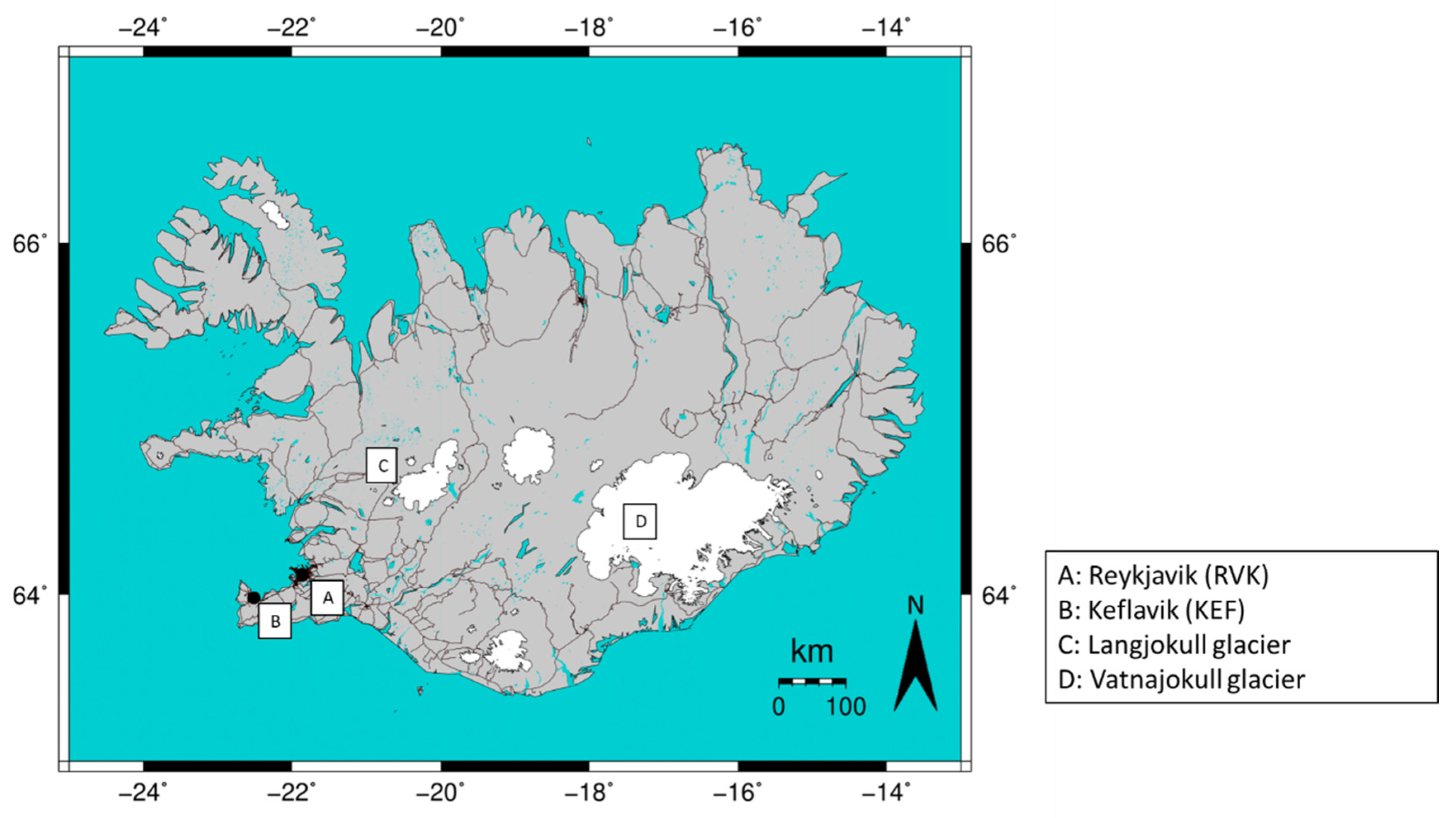
2.1. Observation Sites and Dust Events

Two observation sites are used in this study: Reykjavik (RVK) and Keflavik (KEF). The locations of these sites are displayed in Figure 1. RVK (Figure 1, location A) has the most varied instrumentation. KEF (Figure 1, location B) is the Keflavik International Airport, the main international airport in Iceland. RVK site is 52 m above sea level (asl) and KEF is 51 m asl.

The first selected dust event was observed on 14 and 15 June at RVK, and the second was observed on 31 July and 1 August, at both RVK and KEF. The two dust episodes are named as the June case and the July case accordingly throughout the text. The coordinates and the instruments installed at both sites can be found in

Table 1. The dates, locations and instrumentation available during the two events described in this study.

Start Date	End Date	Location	Latitude (°N)	Longitude (°W)	Lidar	Ceilometer	Other Measurements
2019-06-14	2019-06-15	RVK	64.1275	21.9027	WindCube	CL31	PM10, sun-photometer,
2019-07-31	2019-08-01	RVK	64.1275	21.9027	WindCube	CL31	PM10, sun-photometer
		KEF	63.9829	22.6005	WindCube	CL51	Radio sounding

.

2.2. Instruments

The two Leosphere WindCube Scan 200S Doppler lidars used in this study are both equipped with a depolarization module. The emitted wavelength is 1.54 μm, and the selected spatial resolution is 100 m. The lidar can be operated in various modes, according to the observation purpose: it can measure vertical profiles of the horizontal wind components and vertical velocity with conically shaped velocity-azimuth-display (VAD) scans [15]. Furthermore, the lidars are equipped with a depolarization module for aerosol measurements. In this study, we use the vertical stare for the backscatter coefficient and depolarization ratio measurements and VAD scans for calibration and wind measurements. One system is located at KEF, and the other is installed on a mobile trailer located at RVK. The mobile lidar offers the capability to move the instrument in case of a special event, e.g., a volcanic eruption. During this study, the lidar trailer was stationary at RVK, next to the headquarters of the Icelandic Meteorological Office (IMO).

IMO operates a ceilometer network in Iceland, including seven Vaisala CL31 and two CL51 ceilometers. In addition, two CL51 ceilometers are located at KEF, as part of the Automated Weather Observing System (AWOS) and operated by the airport. Here, we use one CL31 ceilometer that is installed in the mobile trailer, along with the lidar, and one CL51 ceilometer at KEF.

Table 2. The main specifications of the lidars and ceilometers operated in Iceland.

Feature	Lidar	Ceilometer
Model	Windcube 200S	CL31	CL51
Manufacturer	Leosphere	Vaisala	Vaisala
Wavelength (μm)	1.54	0.91	0.91
Maximum detection range (km)	14	7.6	15
Range resolution (m)	100	10	10
Elevation angle (°)	−10–90	90	90
Azimuth angle (°)	0–360	N/A	N/A

summarizes the basic specifications of the lidars and the ceilometers. The main difference between the CL31 and CL51 ceilometers is the different laser pulse energy resulting in a maximum detection range of 7.6 and 15 km, respectively.

Lidars and ceilometers are the main instruments utilized in this study, and the data processing of each will be described in Section 2.3. The wind retrieval of lidar data is described by Yang et al. [6].

In addition to the data from the Doppler lidars and ceilometers, several complementary datasets are applied in this study, depending on the availability at the locations. A Cimel CE-318 sun-photometer, provided by Ludwig Maximilian University of Munich (LMU), Germany, was deployed from July 2018 to September 2019 at IMO headquarters at Reykjavik. From the measured data aerosol optical properties, primarily the aerosol optical depth (AOD) and the Angstrom exponent, can be retrieved.

The Environment Agency of Iceland measures air quality indicators around the country, mostly in urban areas. Here we use the ground-level PM₁₀ (particle matter with a diameter of less than 10 μm) and PM_2.5 (particle matter with a diameter of 2.5 μm or less, also known as fine particles) mass concentrations. They are commonly used as an indicator of air quality around the world. We use the hourly data collected in Njorvasund, Reykjavik, which is about 3.5 km from IMO. The instrument used at this station is a BAM 1020 Continuous Particulate Monitor (MET One Instruments. Inc., Grants Pass, OR, USA).

There are several webcams mounted on the IMO headquarters’ building, taking pictures automatically on an hourly basis. These webcams are used for visibility examination.

The mobile lidar trailer was placed close to IMO’s measurement field which has an automatic weather station (AWS). An AWS is also located at KEF. From both AWS we use the 10 min relative humidity measurements. These measurements have an up to ±5% uncertainty, the highest when relative humidity above 95%, which means that the recorded relative humidity may exceed 100%.

At KEF, IMO operates a radio sounding station where a radiosonde is launched twice per day, at noon and midnight. NOAA’s HYSPLIT [41] model is used to calculate the backward trajectory of the dust events to estimate its possible origin. The availability of the dataset for online download can be found in Section 7 of Supplementary Materials.

2.3. Lidar and Ceilometer Data Processing

The primary output of Leosphere WindCube lidar is the carrier to noise ratio (CNR), which is directly related to the received backscatter signal [42]. Besides CNR, the output also includes radial wind speed, relative backscatter coefficient (β), and depolarization ratio (δ). To obtain the relative backscatter, an automatic calibration can be applied. However, this automatic calibration is not always reliable due to the change of calibration parameters with atmospheric conditions. In addition, the automatic retrieval of the depolarization ratio sometimes has large gaps, due to the mechanical problems of the polarizer. This can cause issues in the retrieval. Thus, we calculate the backscatter coefficient and the depolarization ratio from the raw output CNR. Here an overview of the processing is given. For the ceilometer, we followed a relatively mature path to calibrate the data, with some correction made by us. We also used Klett inversion to retrieve particle backscatter coefficient profiles. In the Supplementary Materials, we present the calculation and lidar data screening in detail.

2.3.1. Lidar Data Processing: Backscatter Coefficient

Leosphere WindCube scanning lidars usually focus the emitted beam at a specific range to maximize the detection distance. This has little impact on wind measurements, but it will cause an artificial peak in the attenuated backscatter coefficient profiles—this is referred to as the focal effect. With a known telescope function, the focal effect can be corrected. The telescope function varies little for the solid-state WindCube scanning lidars. However, strong atmospheric turbulence or moving a lidar can change the focus distance. The lidar can be scheduled to calibrate the backscatter profile automatically. This works under the assumption of homogeneous aerosol load during the calibration scan, along with time and range. Typically, low elevation scans over a homogeneous surface are programmed to calculate the telescope function. Fit parameters of this function are then stored in the lidar database and used to calibrate any subsequent backscatter profile. However, the automatic calibration is not always accurate, especially if the homogeneity criterium is not met during a pre-scheduled calibration scan.

Here we used a manual approach [43] to calibrate lidar data and retrieve the relative backscatter coefficient from CNR. The advantage is, that the scan used to calculate the telescope function is verified for homogeneity. The CNR value is a direct lidar output, which depends on the concentration of aerosols in the atmosphere which backscatter the emitted laser light. The retrieval of the relative backscatter coefficient is described in detail in Section S2 of Supplementary Materials.

The uncertainties of CNR measurements have been estimated by calculating the power spectrum density (PSD) for each range. The calculated uncertainties are within 1 dB in the June case and 0.5 dB in the July case. More detailed information can be found in the Supplementary Materials.

2.3.2. Lidar Data Processing: Depolarization Ratio

The detection of depolarization ratio is widely used by advanced lidar systems to classify aerosol types. Typically, linearly polarized radiation is emitted and two detection channels are implemented: one perpendicular to the plane of the laser, and one parallel or one total (parallel and perpendicular). With calibrated two channel observations [44] the particle linear depolarization ratio ${\delta }_p$ can be determined and used. Together with the lidar ratio and/or the color ratio, one can distinguish different aerosol types, e.g., Saharan dust, marine aerosols, biomass burning aerosol, and volcanic ash [8,10,45,46].

While the ceilometers do not provide depolarization information, a depolarization ratio is measured by the Doppler lidar. Using the co-polar and cross-polar CNR signals, the depolarization ratio profiles [47] can be computed from lidar measurements. However, as the main application of the WindCube lidar is the monitoring of the wind field [15], the depolarization ratio provided has not undergone extensive validation, so that the obtained numbers can only be treated as a qualitative approximation: discrimination between spherical and non-spherical particles is feasible but discrimination between different types of non-spherical particles is not possible. The detailed procedure of depolarization ratio retrieval is presented in Section S3 of Supplementary Materials.

Without a correct calibration of the depolarization channel, it is difficult to provide a quantitative measurement of aerosols. Instead, the measured δ can be treated as a reference: higher δ value means the scatterers are more likely to be non-spherical particles. The background value within the boundary layer and cloud layer is predominantly below 0.2 on a relatively clear day. An example is displayed on data acquired on 28 July 2019 (Figure S2 (Supplementary Materials)). The wavelength of lidar also needs to be taken into account. The wavelength of the Doppler wind lidars we use in Iceland is 1.54 µm, while most other aerosol studies use lidars measuring in the wavelength range from 355 nm to 1064 nm [8,10]. The strength of the polarization process partly depends on the particle size relative to the wavelength, as well as the particles’ deviation from the spherically symmetrical shape [9]. The measured depolarization ratio is mostly wavelength-independent, but a few studies (e.g., [10,14]) found a dependency in the boundary layer.

Although there are a lot of studies using lidar to classify aerosols with depolarization ratio measurements (some combined with lidar ratio and/or colour ratio), other studies (e.g., [48,49]) suggest that the relative humidity (RH) could have a large impact on the depolarization ratio and analyzing results without considering the relative humidity could introduce uncertainties. The reason for this is that hygroscopic, non-spherical particles can absorb water vapour when relative humidity increases and changes to more spherical shape. In addition, the size of the particle may also increase, resulting in a higher backscatter coefficient and also altering the lidar ratio. The visibility, or the extinction term of lidar measurements, may also be highly sensitive to the change in relative humidity [14,15,50]. These studies suggest that relative humidity can have a significant impact on lidar backscatter and depolarization measurements.

In this study, we occasionally identify vertical stripes from the cross-section plot of retrieved lidar backscatter coefficients and depolarization ratios, which are caused by missing profiles. These can be fixed by filtering the data and averaging. Detailed information can be found in Section S4 of the Supplementary Materials.

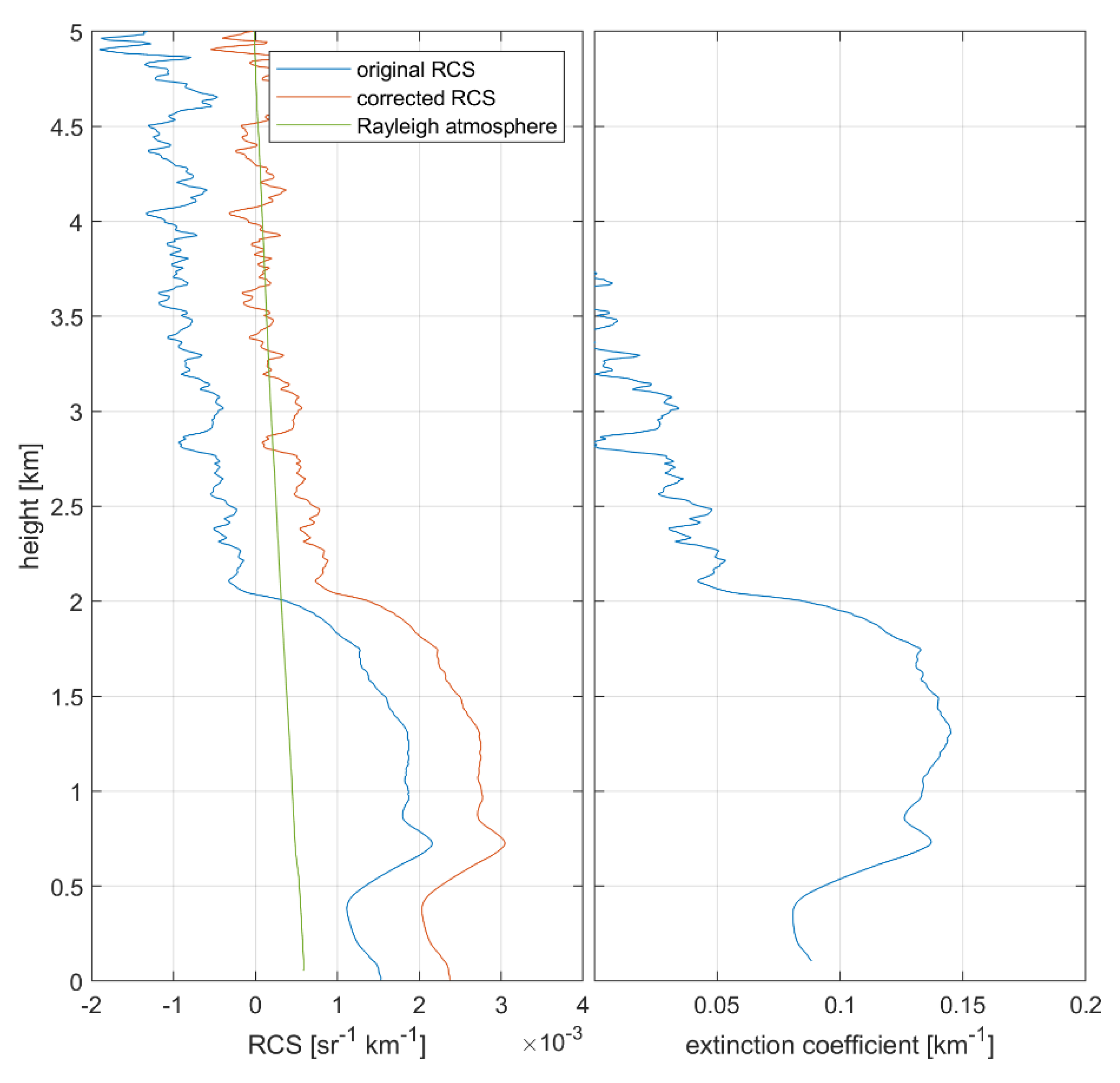
2.3.3. Ceilometer Data Processing

According to the manual [51] of CL31, the output of the ceilometer is attenuated backscatter coefficient ${\beta }^{*}$. Considering the lidar constant in lidar equation is unknown, it would make sense to treat the attenuated backscatter output as “reported range corrected signal (RCS)” ($P\left(r\right)r^2$). The CL31 ceilometer data processing procedure has been studied and here we mainly follow the method of Kotthaus et al. [52]. A dark measurement has been applied to remove the instrument related background signals $P^{bgi}\left(r\right)$. The details of dark measurements can be found in Section 5 of Supplementary Materials. The corrected profile $\widehat{P}{r}^2$ is found to be negative in certain ranges, which is unrealistic. We observed this in several cases, e.g., the June case. According to the communication with the manufacturer, this is instrument-related and can be corrected by adding a constant. Here we use a cosmetic shift constant $F^{CS}$:

$$RC{S}_{corrected}=\widehat{P}{r}^2+F^{CS}$$

(1)

Without an elevated aerosol layer, the atmosphere above the boundary layer is considered to be nearly aerosol free. We can estimate $F^{CS}$ based on this assumption. In this study, we use $F^{CS}=1\times {10}^{-3} {\mathrm{km}}^{-1}{ \mathrm{sr}}^{-1}$ for the data in the June case, but $F^{CS}=0 {\mathrm{km}}^{-1}{ \mathrm{sr}}^{-1}$ in the July case, while the signal at altitudes in the aerosol-free atmosphere is close to zero as expected. We also compare the ceilometer data with data of a sun-photometer, which is co-located to the ceilometer/lidar trailer and calibrated and validated by AERONET. The sun-photometer provides the aerosol optical depth (AOD) at wavelength 1020 nm which can be used to calibrate the ceilometer measurement. AOD is the integration of the particle extinction coefficient ${\alpha }_p$, as the molecular backscatter coefficient ${\beta }_m$ and the extinction coefficient ${\alpha }_m$ are time-independent. With a fixed lidar ratio $S_p$, we can assume the integration of ${\beta }^{*}$is proportional to AOD, and AOD retrieved from the ceilometer should agree with sun-photometer measurements. Here we use a factor C to scale ceilometer and sun-photometer measurement:

$$AO{D}_{sun-photometer 1020 \mathrm{nm}}=\frac{S_p}{C}{\displaystyle \int }{\beta }^{*}\left(r\right)$$

(2)

when there are no clouds, factor C is quite stable (Figure S4 (Supplementary Materials)). Excluding points when there are clouds, averaging the results we have factor C = 1.09.

In summary, here we correct the ceilometer data from the original RCS using:

$$RC{S}_{corrected}=\frac{1}{C}\left(P\left(r\right)-P^{bgi}\left(r\right)\right)r^2+F^{CS}$$

(3)

The whole correction procedure is demonstrated in Figure 2.

With the corrected RCS profile, we can use the Klett inversion method [53] to retrieve ${\beta }_p$ profile and the result should agree with sun-photometer (Figure 2, right). We use the backward Klett inversion method, with the aerosol-free reference height, where ${\beta }_p=0$ and determined by Rayleigh calibration [54]. Figure 2 is an example where the reference height is determined at around 3.7 km. The green line in Figure 2 shows the molecular signal, which is generated by calculating the molecular extinction coefficient ${\alpha }_m$ based on the radiosonde measurement made at Keflavik, which is 45 km southwest of Reykjavik. The corrected RCS profile (orange line) agrees well with the molecular contribution at high altitudes, i.e., aerosol free conditions.

3. Results

Several dust events were observed in the summer of 2019, and they can be identified from the PM concentration measurements (Figure 3). We selected two events observed in the middle of June and at the end of July 2019. On 14 June, a dust storm was observed in the Reykjavik area. The weather observations recorded low visibility and hazy weather. We compared the backscatter coefficients and depolarization ratios from the ceilometer and wind lidar at RVK. On 31 July, another dust storm was observed in Reykjavik, as well as in Keflavik. In this case, we studied both the ceilometer and lidar observations at RVK and KEF.

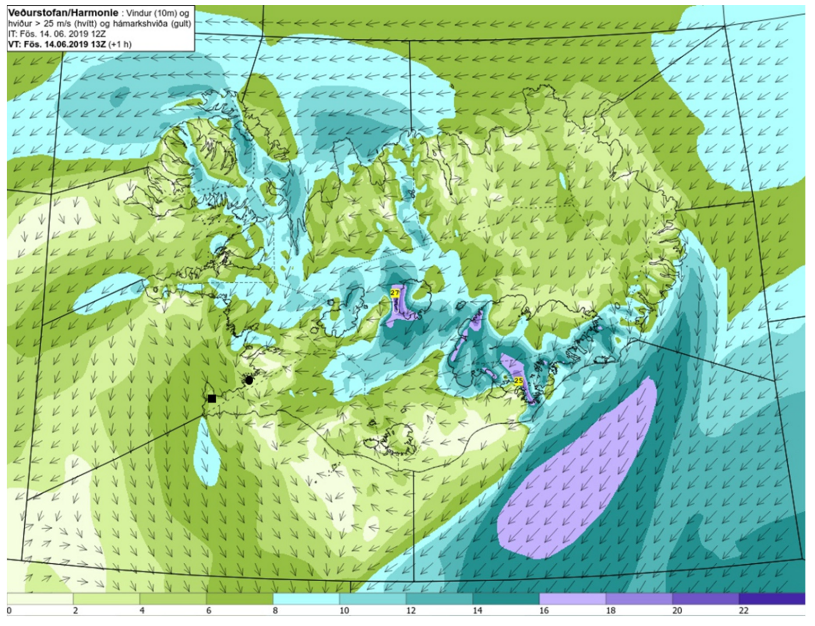
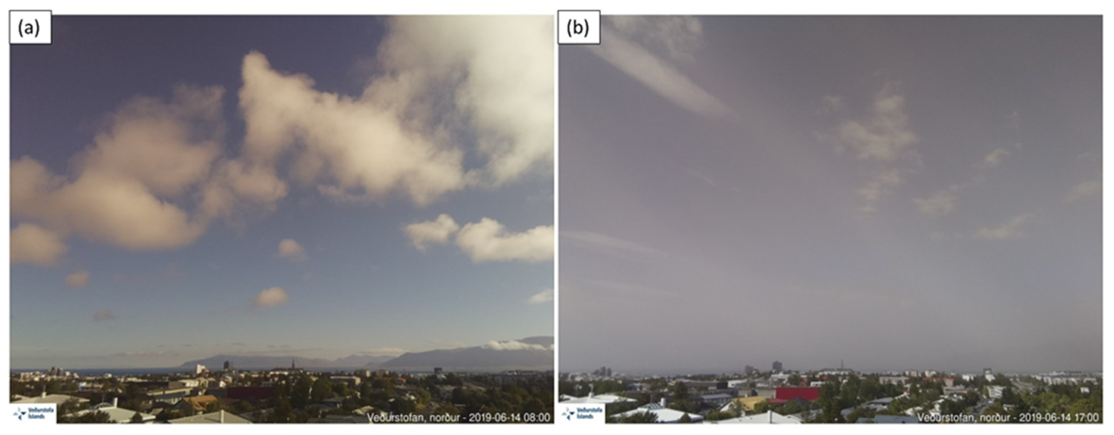
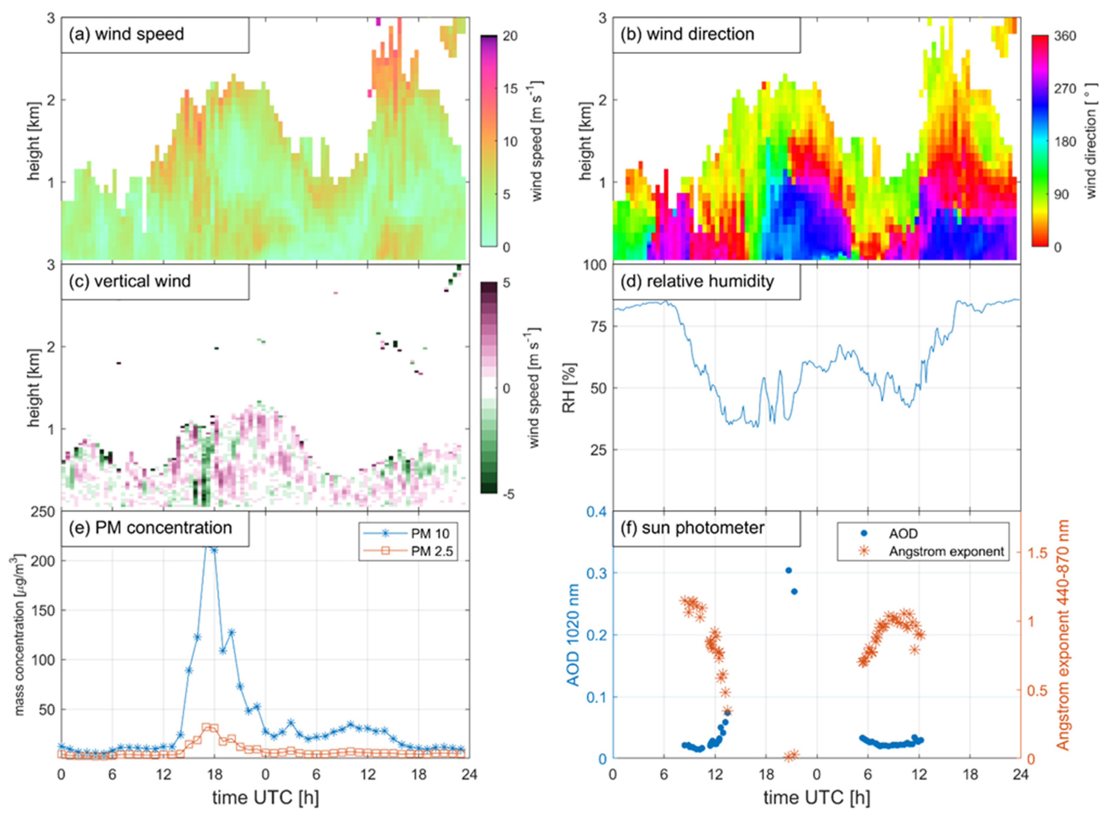
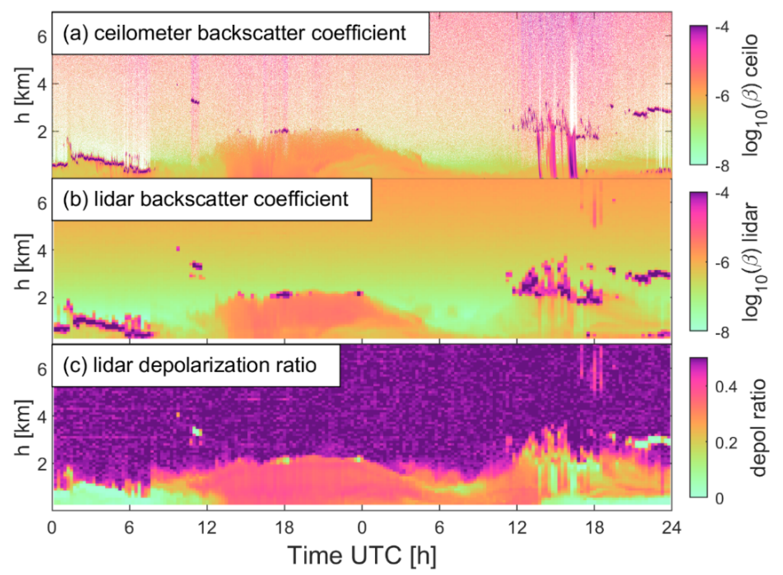
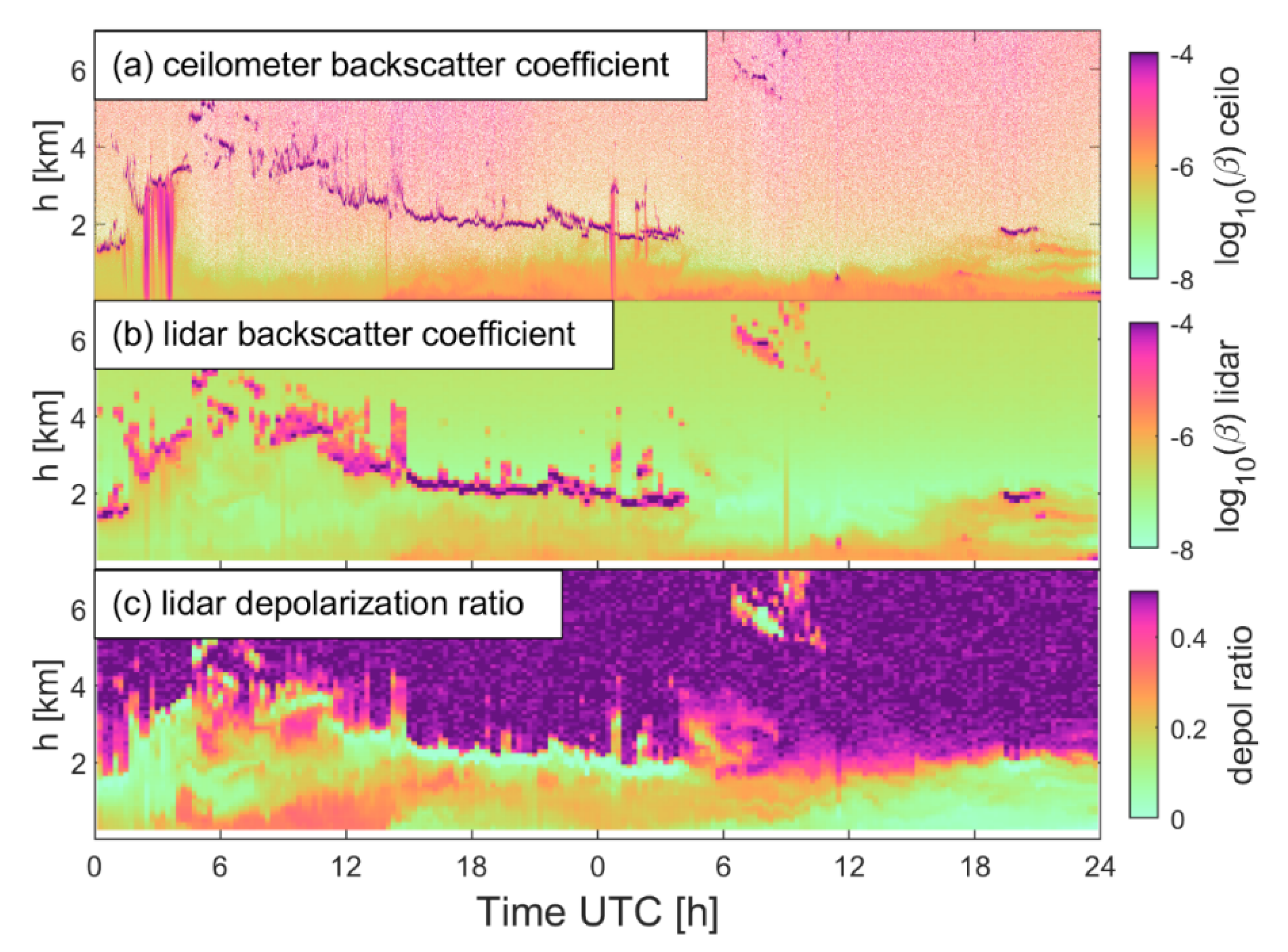
3.1. The June Case (14 June and 15 June)

On 14 June 2019, the weather in Reykjavik was dry with winds from the north-east. Figure 4 shows the 1-h forecast made at 12:00 UTC by IMO, which illustrates the weather conditions. A dust storm passed through Reykjavik in the afternoon, moving from the northeast. According to the HYSPLIT trajectory simulation and weather conditions, the origin of the dust is considered to be at Lake Hagavatn, a dry lake on the south of Langjokull glacier (Figure 1, location C). The dust storm could be seen clearly via the web cameras at IMO. From the camera at IMO pointing north (Figure 5), Mt. Esja, in ~10 km distance was visible in the morning. During the dust event, the visibility decreased and Mt. Esja disappeared. Weather observations showed dust from 15:00 UTC to 21:00 UTC (one report every three hours). The air quality dropped at the same time. PM₁₀ and PM_2.5 concentration (Figure 6e) started to increase at 14:00 UTC and reached a peak value at 17:00 UTC. The surface wind direction changed from easterly to northerly and finally to westerly in the afternoon of the next day, 15 June. At around 12:00 UTC, 14 June, the dry air from northeast arrived in Reykjavik and PM concentration increased sharply, as well as the AOD and particle size measured from the sun-photometer (Figure 6f). Sun-photometer needs to track the sunlight, which is probably the reason why when the visibility dropped considerably the sun-photometer only acquired two measurements during the dust episode (high PM concentration period) at around 21:20 UTC, 14 June. The atmosphere stayed dry during the whole dust event, from 12:00 UTC on 14 June to 12:00 UTC on 15 June, but was then cleaned by a shower in the afternoon of 15 June.

Figure 7 shows the backscatter coefficient measured by the ceilometer (a) and the lidar (b) as well as the lidar depolarization ratio (c). The lidar data were averaged over 15 min. A strong backscatter signal corresponds to more scatterers in the atmosphere. The regions of very high backscatter coefficient shown in dark purple in Figure 7a,b, found on the morning of 14 June (00:00 to 07:00 UTC) and the evening of 15 June (12:00 to 24:00 UTC) are considered to represent low clouds. The low depolarization ratio in these regions indicates spherical scatterers, such as liquid cloud droplets. Both the lidar and the ceilometer detected an aerosol layer starting from around 12:00 UTC on 14 June. In the evening of 14 June, around 22:00 UTC, the aerosol layer was elevated to around 1 km above the surface and it persists until 15 June around 05:00 UTC, when it subsided again. This aerosol layer represents a layer of suspended dust. In the afternoon of 15 June, showers were observed from 13:00 UTC onwards. The ceilometer is more sensitive to precipitation than the lidar, which is the reason that the showers are not as easily seen in Figure 7b. The washout effect of precipitation is significant, both the backscatter coefficient and the depolarization ratio decreased rapidly after the shower.

Figure 8 shows the 30 min averaged backscatter coefficient (β) and depolarization ratio (δ) during the dust event on 14 June, around 21:20 UTC, when there is sun-photometer measurement available.

The shaded areas show the standard deviation. The blue curve shows the β_p from the ceilometer, which is also retrieved from 30-min-average and 100 m smoothed measurements. The lidar data were validated using the CNR filter, and the signal above 2 km were considered as noise. The β profiles from both instruments show a similar vertical structure, with an elevated layer from 0.7 to 2 km, and the peak value at around 1.4 km. The absolute β value is different between lidar and ceilometer, one reason is the wavelength difference of these two instruments, and more importantly, β_p from ceilometer is the retrieved particle backscatter coefficient while β from lidar is the relative backscatter coefficient, which was not calibrated using AOD. The mean depolarization ratio value for the aerosol layer was around 0.35 in this case, and it was nearly height independent, which means the particle type is constant throughout the profile, and the depolarization ratio is independent of the backscatter coefficient or aerosol concentration. There are two small peaks at around 0.6 km and 1.8 km, which can also be found in the cross-section Figure 6. The peaks can be attributed to the focal effect caused by profile-to-profile changes in the lidar focus.

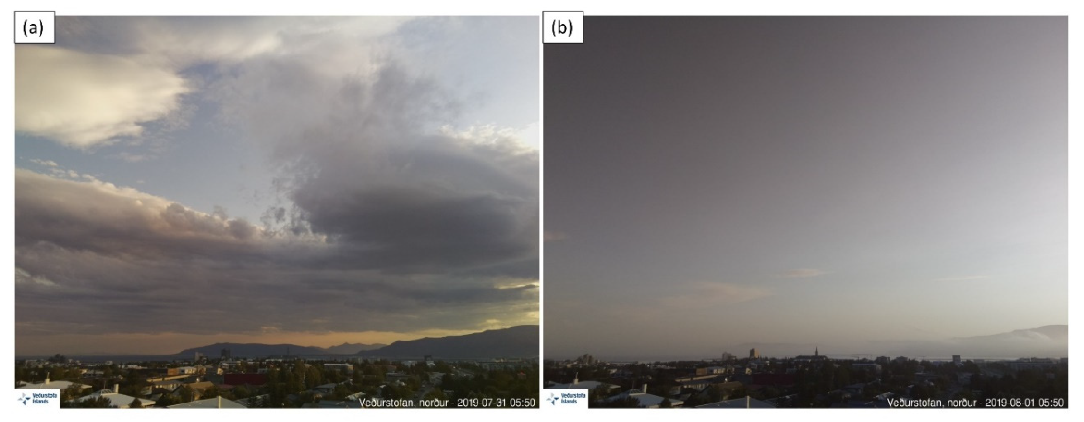
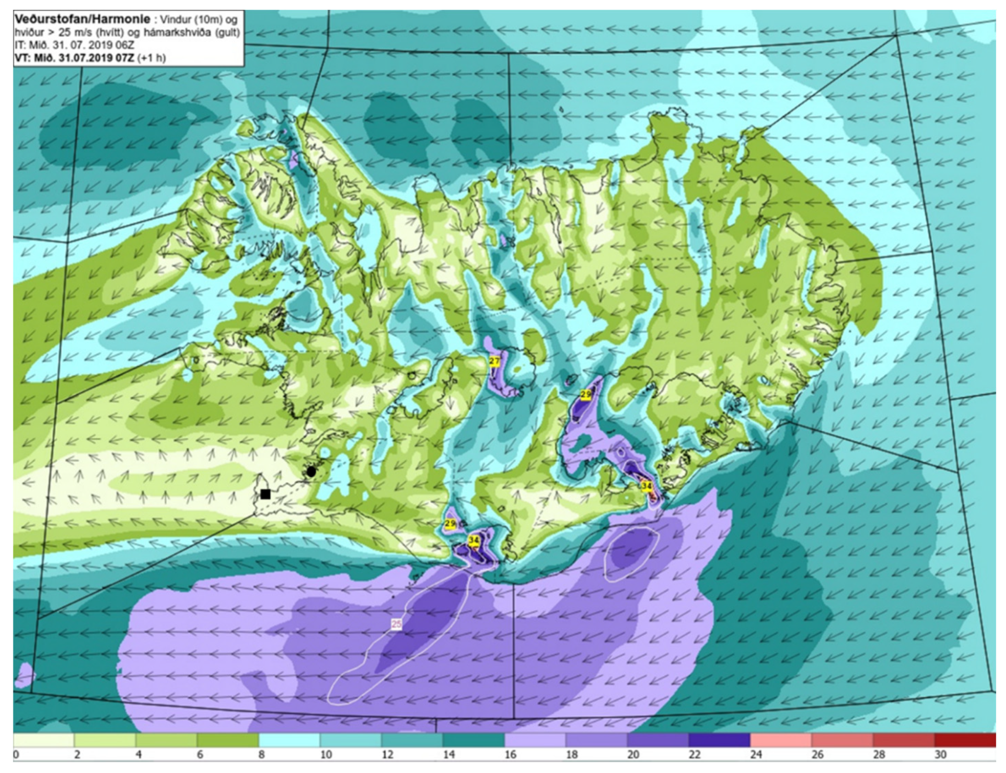
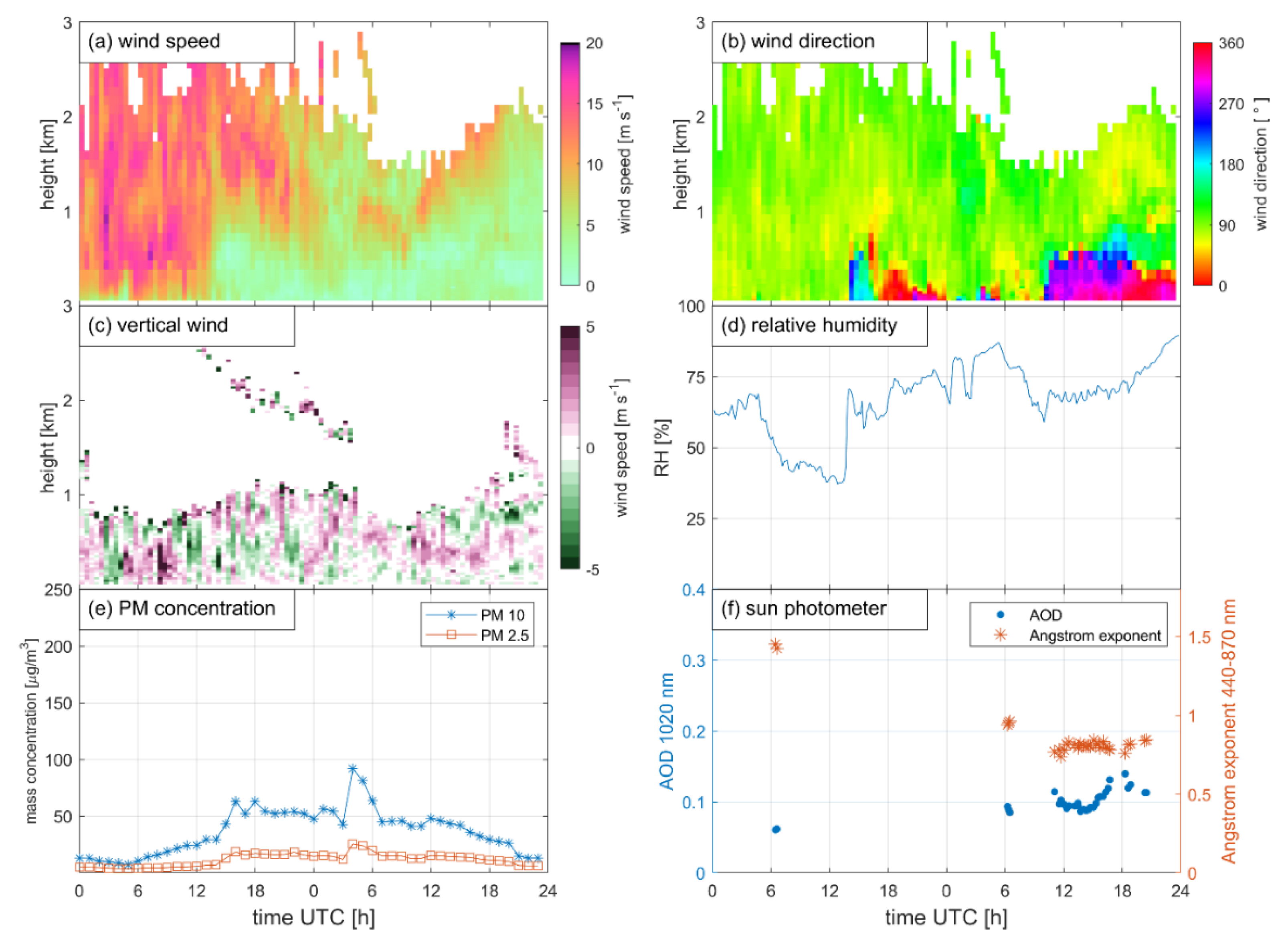
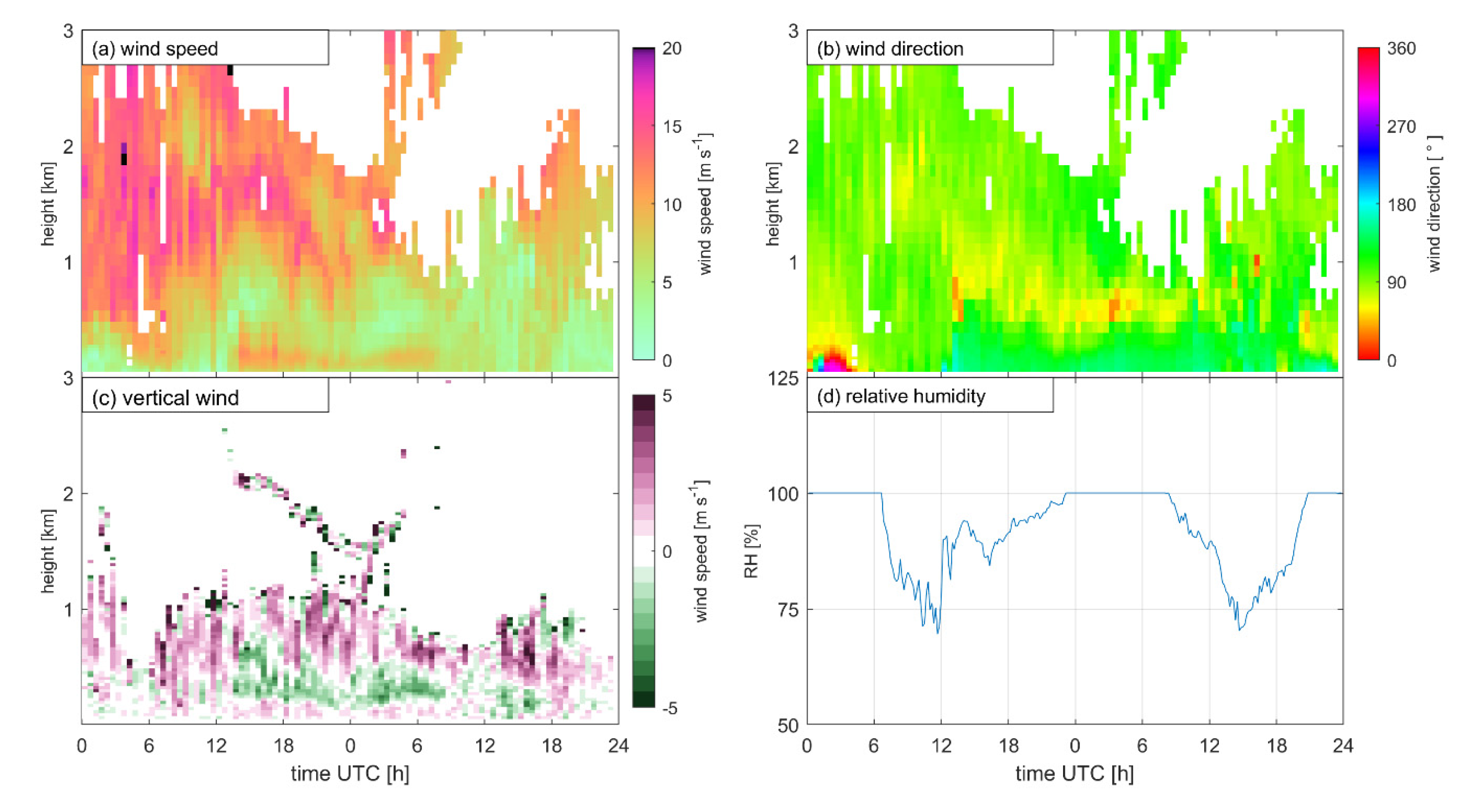
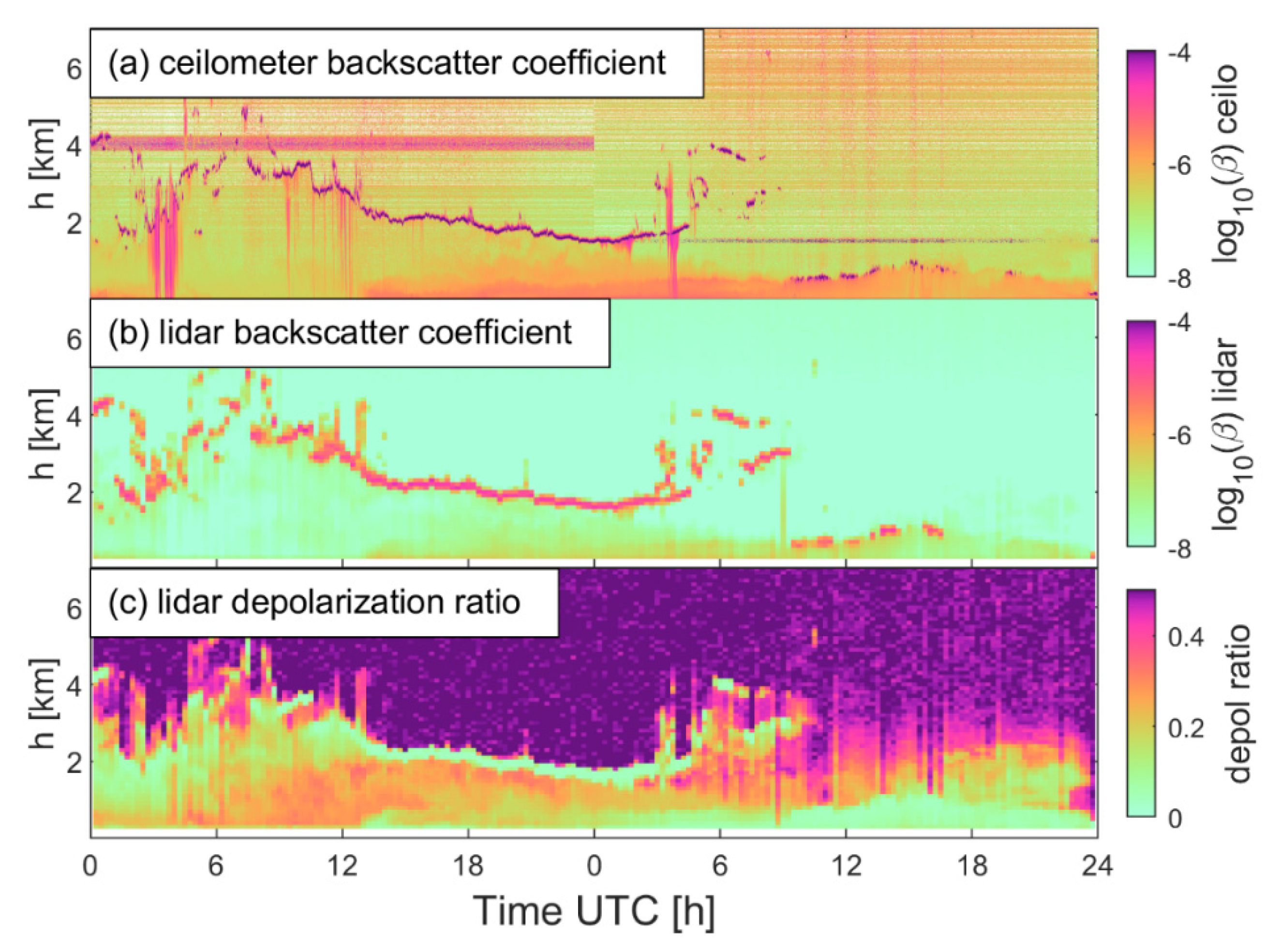
3.2. July Case (31 July and 1 August)

On 31 July 2019, a dust storm reached both Reykjavik and Keflavik airport. The data processing method is the same as in the June case, described in Section 2, but the main difference is that the ceilometer at Keflavik airport was not calibrated. The weather observation registered decreased visibility at 06:00 UTC, 31 July. From 15:00 UTC 31 July to 12:00 UTC 1 August, the 3 hourly weather observation reported haze. The visibility change due to the dust event can be seen in Figure 9, which shows the photos taken by the north-looking webcam installed at IMO headquarters, on 31 July and 1 August, at 05:50 UTC.

As in the June case, Mt. Esja was obscured during this episode. Figure 10 shows the wind conditions on 31 July. Unlike the June case, the wind in the morning of 31 July was easterly (Figure 10), and combining the HYSPLIT and weather conditions, the origin of the dust is considered to be from the west of the Icelandic highlands, on the west of Vatnajokull glacier, the largest ice cap in Iceland (Figure 1, location D). The western highlands are also a common source of Icelandic dust [18,27,55]. PM₁₀ and PM_2.5 concentration in Reykjavik were high from the afternoon of 31 July. They stayed at an elevated level in the afternoon of 31 July (see Figure 11e) and peaked around 05:00 UTC on 1 August. However, compared to the June case, the PM₁₀ concentration is lower. The wind field (Figure 11a,b) changed around 13:00 UTC, 31 July, when the wind direction at low levels (below 700 m) turned from easterly to southerly, and the wind speed decreased as well. At the same time, relative humidity (Figure 11d) increased from below 50% to around 70%. There was no sun-photometer measurement during the peak pollution period, possibly the sun light was blocked by clouds or an aerosol layer (07:00 UTC 31 July to 06:00 UTC 1 August).

However, both AOD and Angstrom exponent was relatively high, which means the particle size was smaller than during the June case. This was in agreement with the PM measurement, as the PM_2.5 concentration was similar, but the PM₁₀ concentration was considerably lower in the July case. The weather at Keflavik (Figure 12) was similar to Reykjavik (Figure 13), except for the wind direction which kept stable on 1 August at KEF, and the relative humidity was higher.

Figure 13 and Figure 14 show the measurements of the ceilometer and lidar backscatter coefficient as well as the lidar depolarization ratio at Reykjavik and Keflavik airport, respectively. The PM concentration increased slightly at around 05:00 UTC on 31 July and then increased more in the afternoon, not decreasing until the end of 1 August. Both ceilometer and lidar backscatter coefficients revealed similar trends; close to the ground, a strong backscatter signal was detected after 13:00 UTC 31 July until the end of 1 August. Precipitation was observed by ceilometer measurements at both sites around 03:00 UTC, 31 July, while the lidar depolarization ratio was low. A layer with a high depolarization ratio was elevated untill 17:00 UTC and decreased slightly after that. Similar observations can be found in Keflavik, where the depolarization ratio was higher in the morning of 1 August, but the backscatter coefficient was low. The horizontal stripes in Figure 12a are instrument related [52], and this ceilometer was not calibrated.

There is no sun-photometer measurement when PM concentration reaches a peak value, so we choose the measurement at around 06:20 1 August, when the AOD is around 0.1, still higher than in clean air (around 0.02), and present the backscatter coefficients and depolarization ratio profiles at the same time (Figure 15). Similar to the June case, lidar $\beta$ and ceilometer ${\beta }_p$ did not fully agree with each other, but here ${\beta }_p$ was higher than $\beta$ at the assumed depolarizing aerosol layer height (<1 km). It can be explained by different particle sizes: as noted, the origin of the two events varies, and the Angstrom exponent, in this case, was much higher than during the June case. The Angstrom exponent value was similar to the one at no-dust level in the June case, which means the size of the particles, in this case, is much smaller. The wavelength of the ceilometer is shorter than lidar, which means the ceilometer is more sensitive to smaller particles than lidar. What should also be noted is that the depolarization ratio profile has a different shape than the backscatter coefficient, which will be discussed in Section 4.

4. Discussion

From the results section, two main topics are discussed: (1) The different results obtained from the June and July case; (2) The differences between the lidar and ceilometer measurements.

4.1. The Difference Between June and July Case

In both cases, dust events occurred during the summertime, but the lidar and ceilometer measurements differ. Firstly, in the June case, the ceilometer ${\beta }_p$ value is lower than the lidar β value, at the level of the dust layer (Figure 8), while in the July case (Figure 15) it is the opposite. Secondly, in the June case, β and δ observations show a similar vertical distribution and temporal evolution (Figure 7), while in the July case they are more varied (Figure 13 and Figure 14). There are several possible explanations: the different dust origins, which may lead to the different physical properties of dust particles, such as shapes and particle size distribution. The origins of both dust event, Lake Hagavatn (June case) and the Western Highlands (July case) are severe erosional areas and common source locations for dust in Iceland [18]. Lake Hagavatn is a dry glacial lake, characterized by more crystalline materials than the volcanic glass that makes up most other Icelandic dust, while the Western Highlands area is covered with silty sediments as well as volcanic materials, and the particles are more spherical than other volcanic ash [18,55]. Figure 16 shows the size distribution measured by the sun-photometer. We used a different sky scenario based on data availability. The particle size in the June case (blue curve) was larger than in the July case (orange curve), and PM concentration measurements gave similar results. As mentioned above, the wavelength of the ceilometer is shorter than that of the lidar, thus the ceilometer is more sensitive to smaller particles, and accordingly, the ceilometer ${\beta }_p$ value in July case is larger.

The different weather conditions should also be considered. With the help of the HYSPLIT model, the dust origins of two cases remained unchanged during the episode accordingly, but in the July case, there was a clear advection of another air mass around 14:00 31 July, when wind field changes and relative humidity increased sharply, and again around 10:00 1 August, while relative humidity in the June case remained low. Figure 17 shows β and δ versus relative humidity in the June and July case. The relative humidity is recorded at the weather station next to the lidar trailer every 10 min, 2 m above the surface; β and δ only use the first range gate (200 m) measurements, averaged every 10 min. The colour indicates the PM₁₀ concentration. If we assume PM₁₀ concentration is high during the dust event, dust and non-dust observations in the June case can be easily distinguished in Figure 17c. In general, there is a clear negative correlation between δ and RH, but high PM₁₀ measurements associated with high δ (>0.25) have a different pattern, compared to low PM₁₀ observations. The low PM₁₀ dots are considered as a non-dust group and have a similar trend with [48] observation. In the July case, the measurements can be divided into three groups: (1) low PM group, which is similar to the non-dust group in the June case, also shows a negative correlation between δ and RH; (2) the relative high RH (>60%) high δ (>0.25) group, which is similar to the dust group in the June case, but the PM₁₀ concentration is lower, corresponding to the high δ, low β measurement in the morning of 31 July (Figure 13); (3) the relative high RH, mid δ (0.1–0.2) group, which has no significant correlation between RH and δ, could represent the particles that absorbed water vapour. The AOD measurements are around 0.07, which is still higher than the background value (i.e., 0.02), but much lower than the peak value during the June case (0.3). The PM concentration increased in the morning when weather observation reported decreased visibility and the high depolarization ratio suggested a layer of non-spherical particles. A possible explanation is that the depolarization ratio measurements are only sensitive to the shape but not the concentration of aerosols. Thus, in some cases, if the particles are non-spherical with a low concentration, it will be easier to detect them by depolarization ratio than backscatter coefficient. In the morning of 31 July, the aerosol concentration was relatively low, compared to the peak value, so the dust aerosols can easily be observed by the depolarization ratio but not by backscatter coefficient. In the afternoon of 31 July, with increased relative humidity, the particles absorbed water vapour and became more spherical, so the depolarization ratio decreased. However PM concentration increased, which could be a result of transported aerosols accumulation, and naturally, the observed backscatter coefficient increased. To examine the specific relation between RH and lidar measurement, a more advanced lidar can be used which also measures humidity profiles [48,56].

4.2. The Difference Between Lidar and Ceilometer Measurements

As is shown in Figure 8 and Figure 15, the ceilometer ${\beta }_p$ and lidar β profiles do not fully agree with each other but were similar in trend. First, there are two facts we need to keep in mind: (1) the lidars and ceilometers have different wavelengths (1540 nm vs. 910 nm), therefore the results of measuring scatterers with different size distributions are expected to be different; (2) The ceilometer profile is calibrated by Rayleigh curve and retrieved by Klett inversion. In other words, it has removed the effect of Rayleigh scattering from atmospheric molecular and extinction. While the lidar, on the other hand, was calibrated by the focus function, which neglects the impact of extinction. In short, ${\beta }_p$ (for the ceilometer) and β (for the lidar) are different physical variables, with different measuring wavelengths, and accordingly, only their relative distribution can be compared.

Furthermore, an unexpected cosmetic shift of ceilometer profiles occurs in some cases. The $CN{R}_{\perp }$ profiles may occasionally not perform as expected. It is difficult to have a quantitative comparison between these two instruments, but they both detected the aerosol layer similarly and showed similar patterns in the cross-sections and vertical profiles.

5. Conclusions

In this study, two types of active remote sensing systems were used to detect atmospheric aerosols in Iceland. Two Doppler wind lidars (WindCube 200S, Leosphere) with depolarization channels and ceilometers (CL31 and CL51, Vaisala) were deployed in southwest Iceland. The data were supplemented by a sun-photometer (CE318-T, Cimel), webcams, radiosonde measurements, and weather observations, as well as PM concentration measurements, to allow calibration and validation of the remotely sensed aerosols monitoring. The study explores the procedures to process lidar and ceilometer data, which is the first to explore the use of WindCube 200S with depolarization module for aerosol detection and demonstrates the application of the procedure to two dust events that occurred during the summer of 2019. The data are analyzed and compared with observations from the sun-photometer and the PM measurements.

The results reveal that both lidar and ceilometer observations can detect airborne dust particles. The main findings from this study can be summarized as follows:

(1)

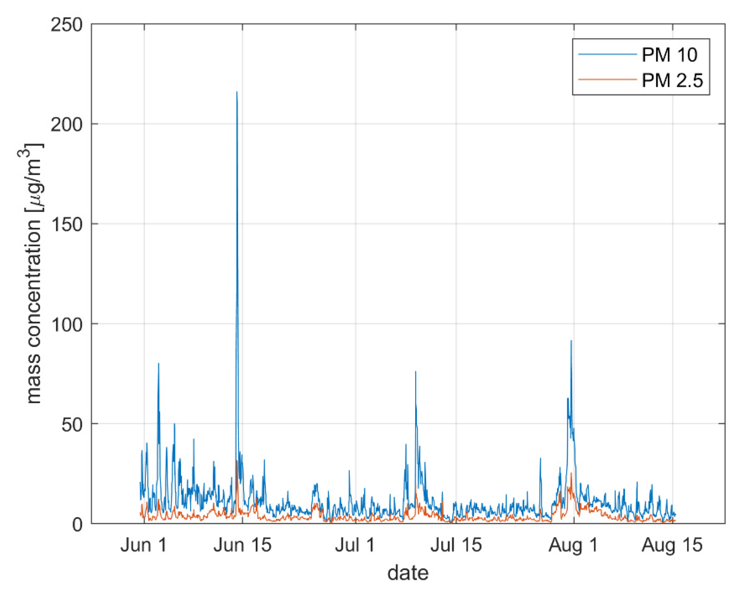
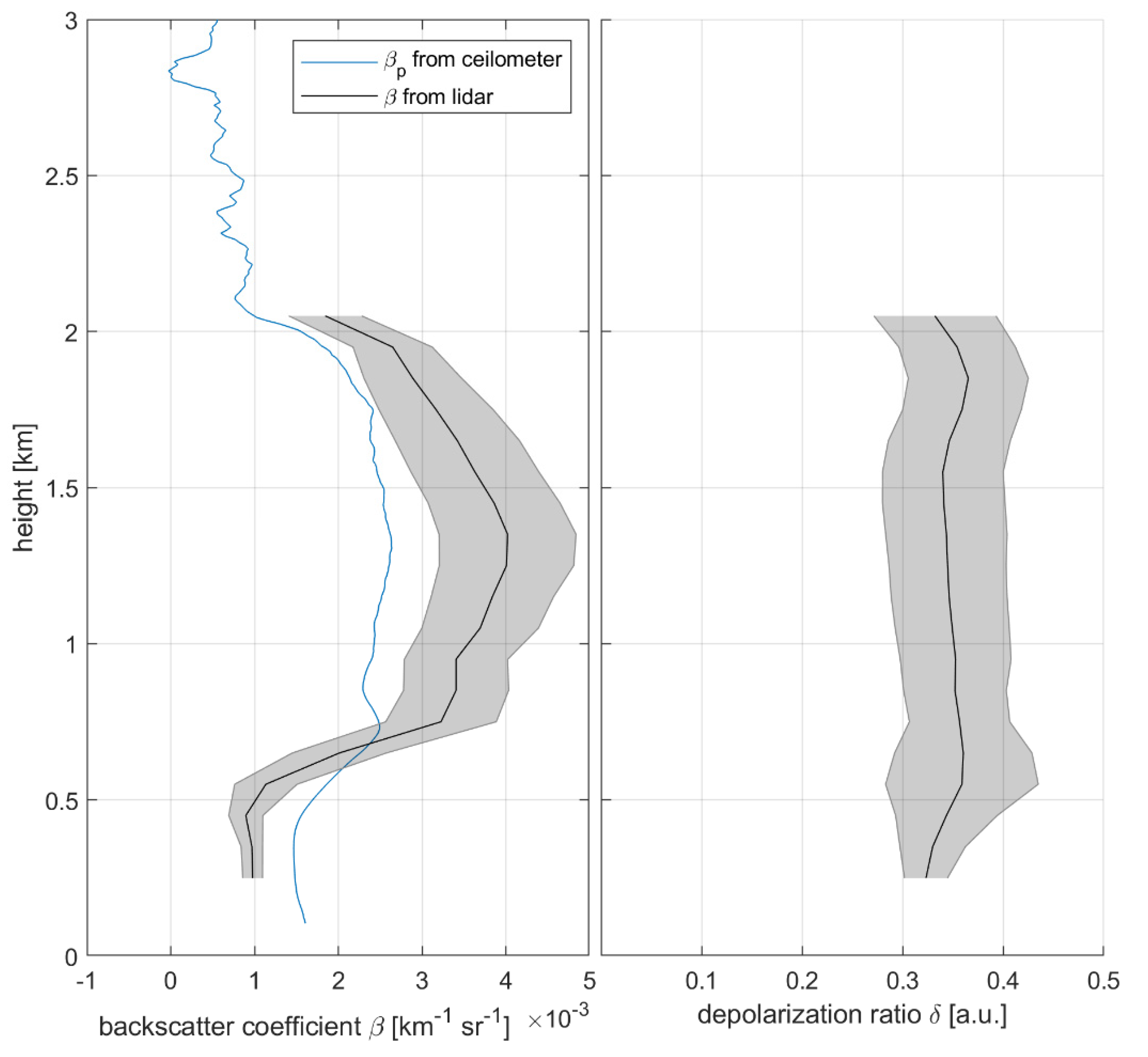
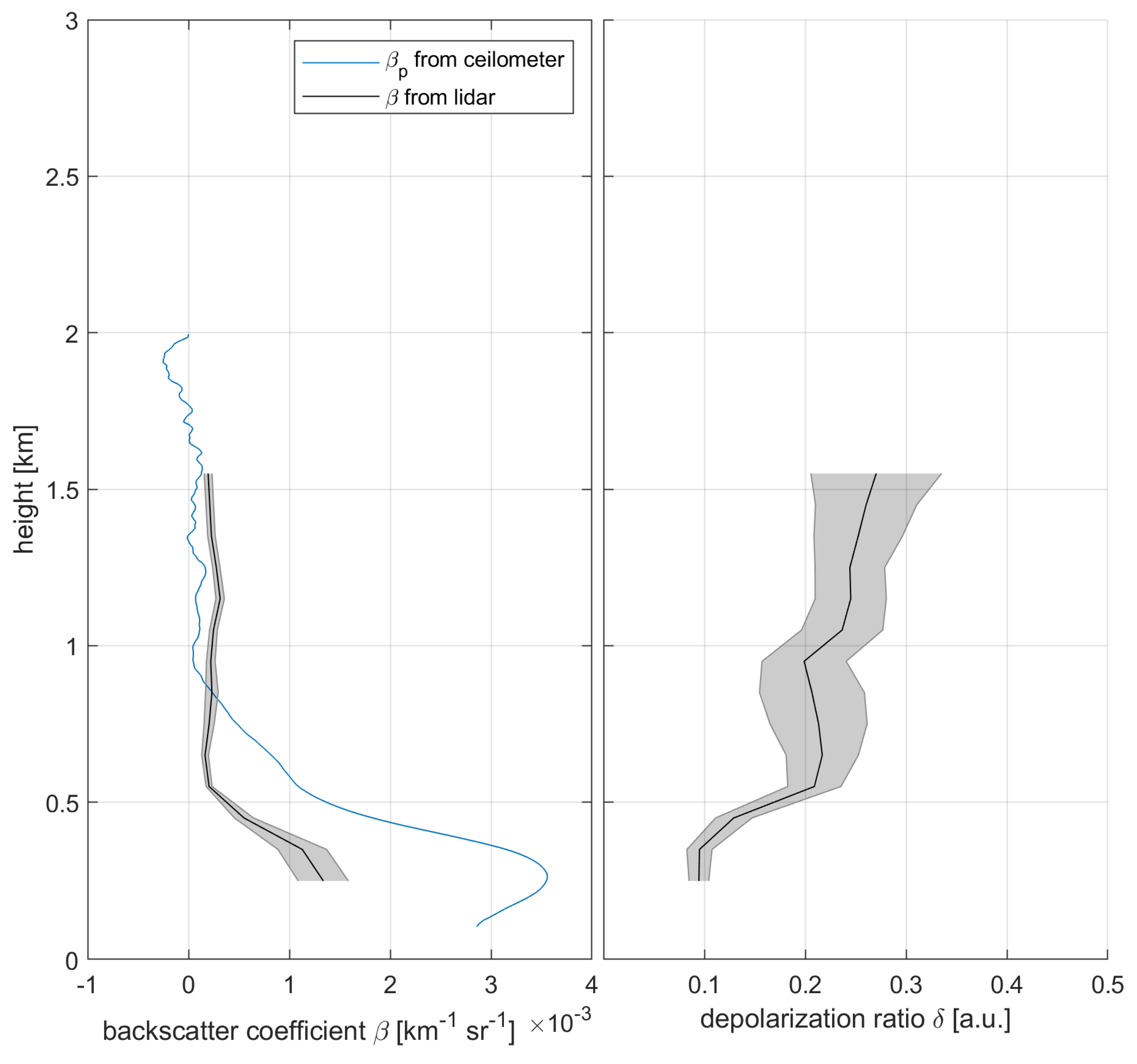
The two instruments consistently reveal similar vertical distributions of aerosols during both dust events. However, the absolute backscatter coefficient profiles are challenging to derive and compare, due to the different nature of the two instruments. Nevertheless, spatial and temporal distributions observed in lidar and ceilometer data are confirmed by observations from other measurements like PM concentration.

(2)

During the processing of lidar and ceilometer data, unrealistic signals have been identified. The $F^{CS}$ factor as an empirical constant has been introduced to correct the unrealistic ceilometer data, which could also be a key source of uncertainty. With the backward Klett inversion method, the particle backscatter coefficients can be retrieved from ceilometer measurements. The lidar data has been calibrated for the focal effect to retrieve the correct relative backscatter coefficient profiles. The difference between lidar and ceilometer can be explained as (i) differences in calibration and data processing procedure, and (ii) different laser wavelengths.

(3)

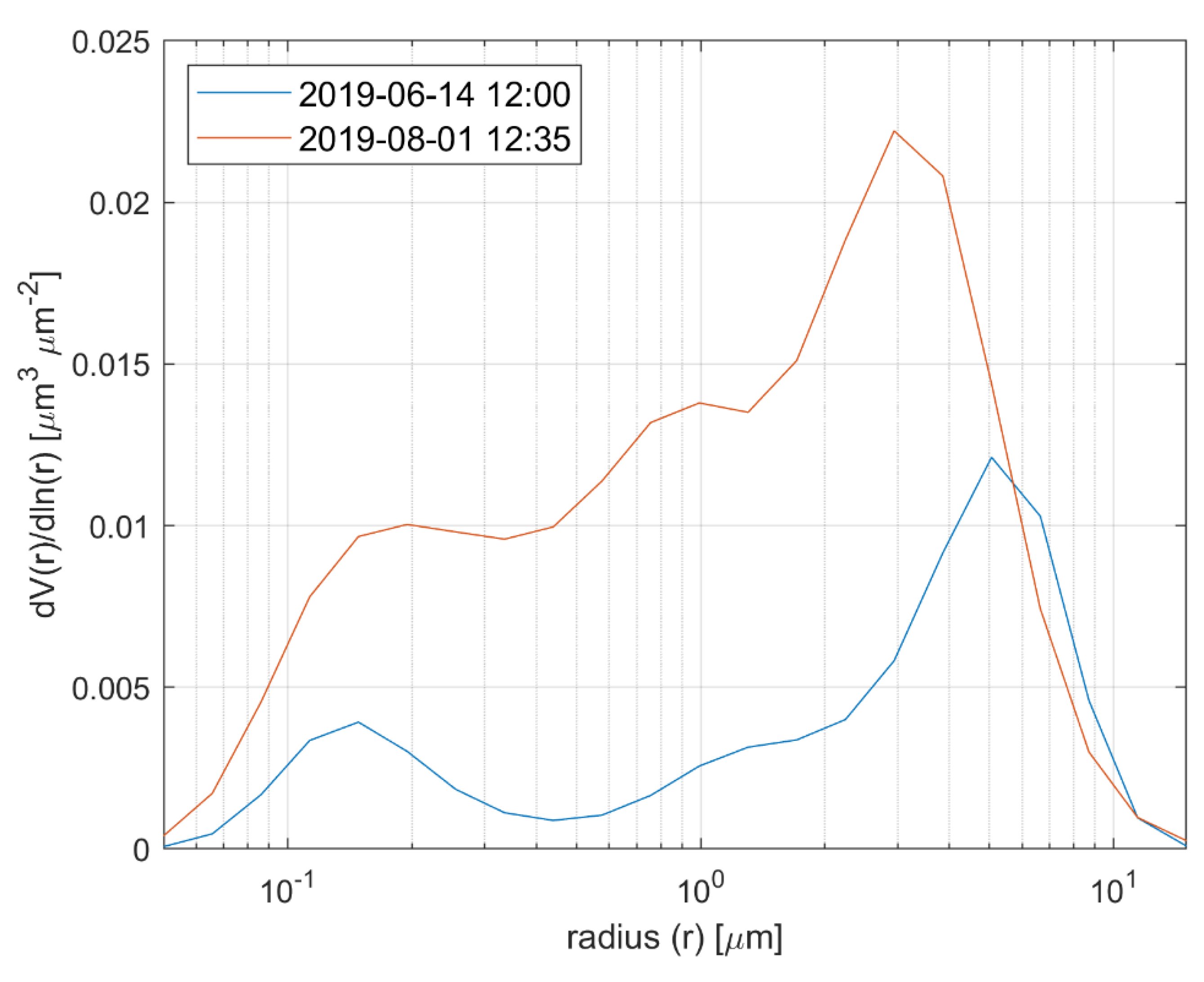
Distinct differences between two dust events have been identified: during the June case, the lidar backscatter coefficient was larger while the ceilometer derived backscatter coefficient was larger during the July case. Particle size distribution retrieved from the sun-photometer revealed that the particle size was larger in the June case, which explains why lidar backscatter coefficients were larger than ceilometers’ in the June case, since the wavelength of Doppler lidar is longer.

(4)

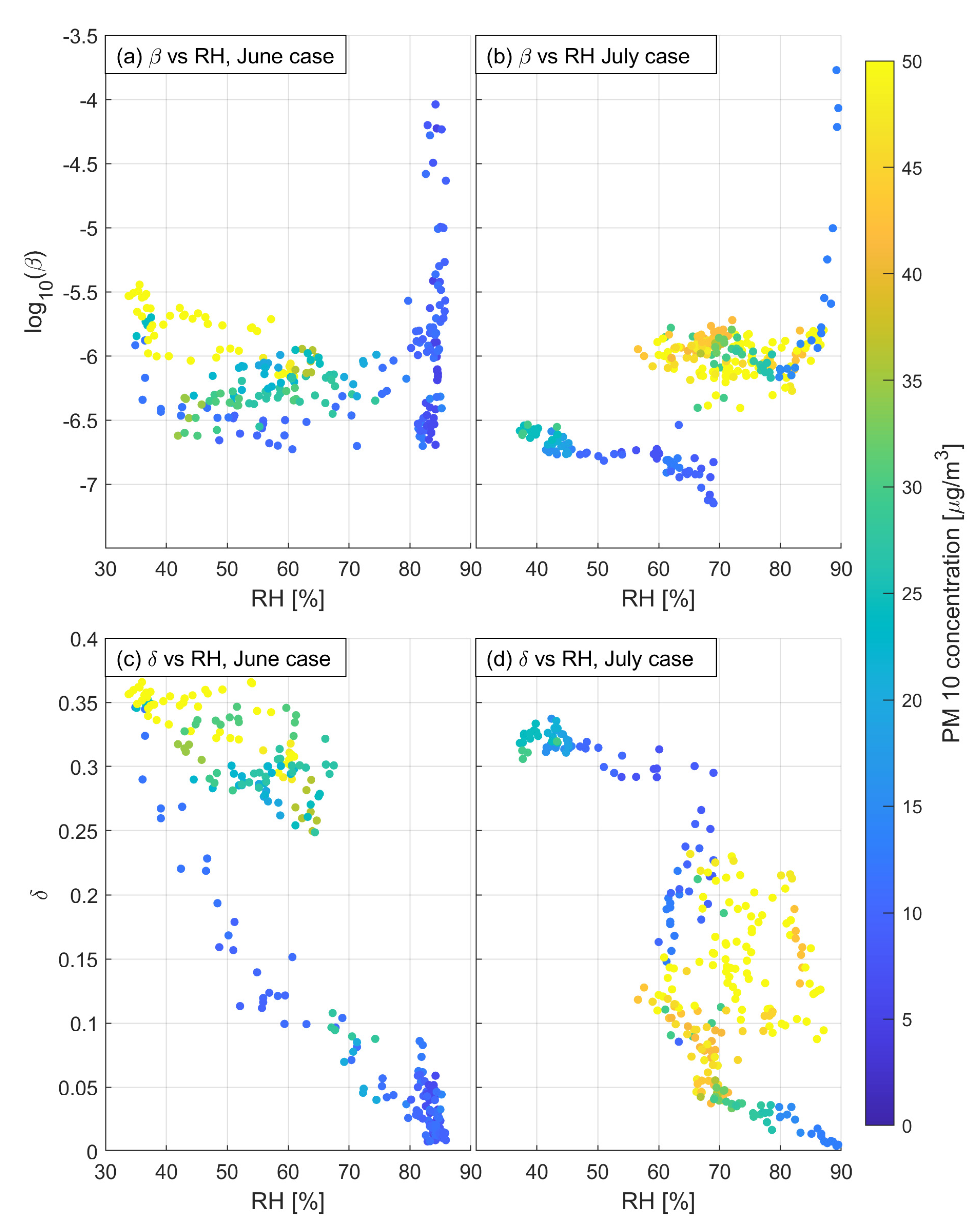
Dust particles are expected to be non-spherical, with the detection of high depolarization ratio and high backscatter coefficients during a dust event. The depolarization ratio observed in this study is distinctively different during the two dust events. In the June case, the depolarization ratio revealed a similar temporal and vertical distribution as the backscatter coefficient, as expected. In the July case, depolarization ratio was high in the morning of 31 July while the backscatter coefficients were relatively low. The backscatter coefficients increased from the afternoon of 31 July but the depolarization ratio was, on the contrary, relatively low. The backscatter coefficients are directly related to the aerosols concentration while the depolarization ratio is less dependent on aerosol concentration. It is determined by the shape of the scatterers, which can be affected by relative humidity. The air remained dry in the June case and both backscatter coefficient and depolarization ratio measurements show a similar pattern. In the July case, relative humidity varied a lot during the two-day observation period. Consequently, we can conclude that when the air is dry and the particle concentration relatively high, the dust can be observed from both backscatter coefficient and depolarization ratio measurements; when the air is dry but particle concentration is low, the aerosols layer may be observed by depolarization ratio but not backscatter coefficients; when air is humid and the particles condense, the aerosols are more obvious from backscatter coefficient compared to depolarization ratio measurements. In general, the relative humidity may have a significant impact on lidar measurements, including backscatter coefficients, depolarization ratio, and also extinction coefficients, which is critical to aviation meteorology [14].

Finally, based on our results we conclude that Doppler wind lidars and ceilometers can provide accurate monitoring of the vertical distribution and temporal evolution of aerosols in Iceland. By installing the instruments on a mobile trailer, the presented data processing approach can be used to alert the local population of severe wind erosions events or ash clouds during volcanic eruptions. Such monitoring of volcanic and sedimentary aerosols can provide important information to decision makers, including an increase in aviation safety in Iceland.

References

1. Gao, H.; Cheng, B.; Wang, J.; Li, K.; Zhao, J.; Li, D. Object Classification Using CNN-Based Fusion of Vision and LIDAR in Autonomous Vehicle Environment. IEEE Trans. Ind. Inform. 2018, 14, 4224–4231. [Google Scholar] [CrossRef]
2. Brook, A.; Ben-Dor, E.; Richter, R. Fusion of hyperspectral images and LiDAR data for civil engineering structure monitoring. In Proceedings of the 2010 2nd Workshop on Hyperspectral Image and Signal Processing: Evolution in Remote Sensing, Reykjavik, Iceland, 14–16 June 2010; pp. 1–5. [Google Scholar]
3. Bilbro, J.; Fichtl, G.; Fitzjarrald, D.; Krause, M.; Lee, R. Airborne Doppler Lidar Wind Field Measurements. Bull. Am. Meteorol. Soc. 1984, 65, 348–359. [Google Scholar] [CrossRef] [Green Version]
4. Chan, P.W. Application of LIDAR-based F-factor in windshear alerting. Meteorol. Z. 2012, 21, 193–204. [Google Scholar] [CrossRef]
5. Gryning, S.-E.; Mikkelsen, T.; Baehr, C.; Dabas, A.; Gómez, P.; O’Connor, E.; Rottner, L.; Sjöholm, M.; Suomi, I.; Vasiljević, N. Measurement methodologies for wind energy based on ground-level remote sensing. In Renewable Energy Forecasting; Elsevier: Cambridge, UK, 2017; pp. 29–56. ISBN 978-0-08-100504-0. [Google Scholar]
6. Yang, S.; Petersen, G.N.; von Löwis, S.; Preißler, J.; Finger, D.C. Determination of eddy dissipation rate by Doppler lidar in Reykjavik, Iceland. Meteorol. Appl. 2020, 27, e1951. [Google Scholar] [CrossRef]
7. Ansmann, A.; Müller, D. Lidar and Atmospheric Aerosol Particles. In Lidar: Range-Resolved Optical Remote Sensing of the Atmosphere; Weitkamp, C., Ed.; Springer Series in Optical Sciences; Springer: New York, NY, USA, 2005; pp. 105–141. ISBN 978-0-387-25101-1. [Google Scholar]
8. Burton, S.P.; Ferrare, R.A.; Hostetler, C.A.; Hair, J.W.; Rogers, R.R.; Obland, M.D.; Butler, C.F.; Cook, A.L.; Harper, D.B.; Froyd, K.D. Aerosol classification using airborne High Spectral Resolution Lidar measurements – methodology and examples. Atmospheric Meas. Tech. 2012, 5, 73–98. [Google Scholar] [CrossRef] [Green Version]
9. Sassen, K. Polarization in Lidar. In Lidar; Weitkamp, C., Ed.; Springer: New York, NY, USA, 2005; Volume 102, pp. 19–42. ISBN 978-0-387-40075-4. [Google Scholar]
10. Groß, S.; Freudenthaler, V.; Wiegner, M.; Gasteiger, J.; Geiß, A.; Schnell, F. Dual-wavelength linear depolarization ratio of volcanic aerosols: Lidar measurements of the Eyjafjallajökull plume over Maisach, Germany. Atmos. Environ. 2012, 48, 85–96. [Google Scholar] [CrossRef] [Green Version]
11. Tuononen, M.; O’Connor, E.J.; Sinclair, V.A.; Vakkari, V. Low-Level Jets over Utö, Finland, Based on Doppler Lidar Observations. J. Appl. Meteorol. Climatol. 2017, 56, 2577–2594. [Google Scholar] [CrossRef]
12. Banakh, V.A.; Smalikho, I.; Köpp, F.; Werner, C. Measurements of Turbulent Energy Dissipation Rate with a CW Doppler Lidar in the Atmospheric Boundary Layer. J. Atmospheric Ocean. Technol. 1999, 16, 1044–1061. [Google Scholar] [CrossRef]
13. Chan, P.W.; Lee, Y.F. Performance of LIDAR- and radar-based turbulence intensity measurement in comparison with anemometer-based turbulence intensity estimation based on aircraft data for a typical case of terrain-induced turbulence in association with a typhoon. J. Zhejiang Univ. Sci. A 2013, 14, 469–481. [Google Scholar] [CrossRef] [Green Version]
14. Gultepe, I.; Sharman, R.; Williams, P.; Zhou, B.; Ellrod, G.; Minnis, P.; Trier, S.; Griffin, S.; Yum, S.S.; Gharabaghi, B.; et al. A review of high impact weather for aviation meteorology. Pure Appl. Geophys. 2019, 176, 1869–1921. [Google Scholar] [CrossRef]
15. Thobois, L.; Cariou, J.P.; Gultepe, I. Review of Lidar-Based Applications for Aviation Weather. Pure Appl. Geophys. 2019, 176, 1959–1976. [Google Scholar] [CrossRef]
16. Münkel, C.; Eresmaa, N.; Räsänen, J.; Karppinen, A. Retrieval of mixing height and dust concentration with lidar ceilometer. Bound.-Layer Meteorol. 2007, 124, 117–128. [Google Scholar] [CrossRef]
17. Wiegner, M.; Madonna, F.; Binietoglou, I.; Forkel, R.; Gasteiger, J.; Geiß, A.; Pappalardo, G.; Schäfer, K.; Thomas, W. What is the benefit of ceilometers for aerosol remote sensing? An answer from EARLINET. Atmospheric Meas. Tech. 2014, 7, 1979–1997. [Google Scholar] [CrossRef] [Green Version]
18. Arnalds, O.; Dagsson-Waldhauserova, P.; Olafsson, H. The Icelandic volcanic aeolian environment: Processes and impacts—A review. Aeolian Res. 2016, 20, 176–195. [Google Scholar] [CrossRef] [Green Version]
19. Ólafsson, H.; Furger, M.; Brümmer, B. The weather and climate of Iceland. Meteorol. Z. 2007, 16, 5–8. [Google Scholar] [CrossRef]
20. Thordarson, T.; Larsen, G. Volcanism in Iceland in historical time: Volcano types, eruption styles and eruptive history-ScienceDirect. J. Geodyn. 2007, 43, 118–152. [Google Scholar] [CrossRef]
21. Budd, L.; Griggs, S.; Howarth, D.; Ison, S. A Fiasco of Volcanic Proportions? Eyjafjallajökull and the Closure of European Airspace. Mobilities 2011, 6, 31–40. [Google Scholar] [CrossRef]
22. Carlsen, H.K.; Gislason, T.; Forsberg, B.; Meister, K.; Thorsteinsson, T.; Jóhannsson, T.; Finnbjornsdottir, R.; Oudin, A. Emergency Hospital Visits in Association with Volcanic Ash, Dust Storms and Other Sources of Ambient Particles: A Time-Series Study in Reykjavík, Iceland. Int. J. Environ. Res. Public. Health 2015, 12, 4047–4059. [Google Scholar] [CrossRef] [Green Version]
23. Goudie, A.S. Desert dust and human health disorders. Environ. Int. 2014, 63, 101–113. [Google Scholar] [CrossRef]
24. Gústafsson, L.E.; Steinecke, K. Airborne contaminants and their impact on the city of Reykjavi’k, Iceland. Sci. Total Environ. 1995, 160–161, 363–372. [Google Scholar] [CrossRef]
25. Saidou Chaibou, A.A.; Ma, X.; Sha, T. Dust radiative forcing and its impact on surface energy budget over West Africa. Sci. Rep. 2020, 10, 12236. [Google Scholar] [CrossRef] [PubMed]
26. Wittmann, M.; Groot Zwaaftink, C.D.; Steffensen Schmidt, L.; Guðmundsson, S.; Pálsson, F.; Arnalds, O.; Björnsson, H.; Thorsteinsson, T.; Stohl, A. Impact of dust deposition on the albedo of Vatnajökull ice cap, Iceland. The Cryosphere 2017, 11, 741–754. [Google Scholar] [CrossRef] [Green Version]
27. Dagsson-Waldhauserova, P.; Arnalds, O.; Olafsson, H. Long-term variability of dust events in Iceland (1949–2011). Atmospheric Chem. Phys. 2014, 14, 13411–13422. [Google Scholar] [CrossRef] [Green Version]
28. Gudmundsson, M.T.; Pedersen, R.; Vogfjörd, K.; Thorbjarnardóttir, B.; Jakobsdóttir, S.; Roberts, M.J. Eruptions of Eyjafjallajökull Volcano, Iceland. Eos Trans. Am. Geophys. Union 2010, 91, 190–191. [Google Scholar] [CrossRef]
29. Petersen, G.N.; Bjornsson, H.; Arason, P. The impact of the atmosphere on the Eyjafjallajökull 2010 eruption plume. J. Geophys. Res. Atmospheres 2012, 117. [Google Scholar] [CrossRef]
30. Rix, M.; Valks, P.; Hao, N.; Loyola, D.; Schlager, H.; Huntrieser, H.; Flemming, J.; Koehler, U.; Schumann, U.; Inness, A. Volcanic SO2, BrO and plume height estimations using GOME-2 satellite measurements during the eruption of Eyjafjallajökull in May 2010. J. Geophys. Res. Atmospheres 2012, 117. [Google Scholar] [CrossRef] [Green Version]
31. Chazette, P.; Dabas, A.; Sanak, J.; Lardier, M.; Royer, P. French airborne lidar measurements for Eyjafjallajökull ash plume survey. Atmospheric Chem. Phys. 2012, 12, 7059–7072. [Google Scholar] [CrossRef] [Green Version]
32. Ansmann, A.; Tesche, M.; Groß, S.; Freudenthaler, V.; Seifert, P.; Hiebsch, A.; Schmidt, J.; Wandinger, U.; Mattis, I.; Müller, D.; et al. The 16 April 2010 major volcanic ash plume over central Europe: EARLINET lidar and AERONET photometer observations at Leipzig and Munich, Germany. Geophys. Res. Lett. 2010, 37. [Google Scholar] [CrossRef] [Green Version]
33. Sicard, M.; Guerrero-Rascado, J.L.; Navas-Guzmán, F.; Preißler, J.; Molero, F.; Tomás, S.; Bravo-Aranda, J.A.; Comerón, A.; Rocadenbosch, F.; Wagner, F.; et al. Monitoring of the Eyjafjallajökull volcanic aerosol plume over the Iberian Peninsula by means of four EARLINET lidar stations. Atmospheric Chem. Phys. 2012, 12, 3115–3130. [Google Scholar] [CrossRef] [Green Version]
34. Wiegner, M.; Gasteiger, J.; Groß, S.; Schnell, F.; Freudenthaler, V.; Forkel, R. Characterization of the Eyjafjallajökull ash-plume: Potential of lidar remote sensing. Phys. Chem. Earth Parts ABC 2012, 45–46, 79–86. [Google Scholar] [CrossRef]
35. Prospero, J.M.; Bullard, J.E.; Hodgkins, R. High-Latitude Dust Over the North Atlantic: Inputs from Icelandic Proglacial Dust Storms. Science 2012, 335, 1078–1082. [Google Scholar] [CrossRef] [PubMed]
36. Dagsson-Waldhauserova, P.; Renard, J.-B.; Olafsson, H.; Vignelles, D.; Berthet, G.; Verdier, N. Duverger Vertical distribution of aerosols in dust storms during the Arctic winter. Sci. Rep. 2019, 9, 1–11. [Google Scholar] [CrossRef] [PubMed]
37. Liao, H.; Jing, H.; Ma, C.; Tao, Q.; Li, Z. Field measurement study on turbulence field by wind tower and Windcube Lidar in mountain valley. J. Wind Eng. Ind. Aerodyn. 2020, 197, 104090. [Google Scholar] [CrossRef]
38. Stephan, A.; Wildmann, N.; Smalikho, I.N. Effectiveness of the MFAS Method for Determining the Wind Velocity Vector from Windcube 200s Lidar Measurements. Atmospheric Ocean. Opt. 2019, 32, 555–563. [Google Scholar] [CrossRef]
39. Statistics Iceland Population by Municipality, Sex, Citizenship and Quarters 2010–2020. Available online: http://px.hagstofa.is/pxis/pxweb/is/Ibuar/Ibuar__mannfjoldi__1_yfirlit__arsfjordungstolur/MAN10001.px/table/tableViewLayout1/?rxid=c9d9c074-79f2-40c2-8a30-5479757324ba (accessed on 5 October 2020).
40. IMO Tíðarfar í (Monthly Report of) September 2019. Available online: https://www.vedur.is/um-vi/frettir/tidarfar-i-september-2019#sumar (accessed on 1 October 2020).
41. Stein, A.F.; Draxler, R.R.; Rolph, G.D.; Stunder, B.J.B.; Cohen, M.D.; Ngan, F. NOAA’s HYSPLIT Atmospheric Transport and Dispersion Modeling System. Bull. Am. Meteorol. Soc. 2015, 96, 2059–2077. [Google Scholar] [CrossRef]
42. Boquet, M.; Royer, P.; Cariou, J.-P.; Machta, M.; Valla, M. Simulation of Doppler Lidar Measurement Range and Data Availability. J. Atmospheric Ocean. Technol. 2016, 33, 977–987. [Google Scholar] [CrossRef]
43. Preißler, J.; Leosphere Inc., Saclay, France. Personal communication, 2020.
44. Freudenthaler, V.; Esselborn, M.; Wiegner, M.; Heese, B.; Tesche, M.; Ansmann, A.; MüLLER, D.; Althausen, D.; Wirth, M.; Fix, A.; et al. Depolarization ratio profiling at several wavelengths in pure Saharan dust during SAMUM 2006. Tellus B Chem. Phys. Meteorol. 2009, 61, 165–179. [Google Scholar] [CrossRef] [Green Version]
45. Ansmann, A.; Seifert, P.; Tesche, M.; Wandinger, U. Profiling of fine and coarse particle mass: Case studies of Saharan dust and Eyjafjallajökull/Grimsvötn volcanic plumes. Atmospheric Chem. Phys. 2012, 12, 9399–9415. [Google Scholar] [CrossRef] [Green Version]
46. Groß, S.; Tesche, M.; Freudenthaler, V.; Toledano, C.; Wiegner, M.; Ansmann, A.; Althausen, D.; Seefeldner, M. Characterization of Saharan dust, marine aerosols and mixtures of biomass-burning aerosols and dust by means of multi-wavelength depolarization and Raman lidar measurements during SAMUM 2. Tellus B Chem. Phys. Meteorol. 2011, 63, 706–724. [Google Scholar] [CrossRef]
47. Royer, P.; Boquet, M.; Cariou, J.-P.; Sauvage, L.; Parmentier, R. Aerosol/Cloud Measurements Using Coherent Wind Doppler Lidars. EPJ Web Conf. 2016, 119, 11002. [Google Scholar] [CrossRef] [Green Version]
48. Haarig, M.; Ansmann, A.; Gasteiger, J.; Kandler, K.; Althausen, D.; Baars, H.; Radenz, M.; Farrell, D.A. Dry versus wet marine particle optical properties: RH dependence of depolarization ratio, backscatter, and extinction from multiwavelength lidar measurements during SALTRACE. Atmospheric Chem. Phys. 2017, 17, 14199–14217. [Google Scholar] [CrossRef] [Green Version]
49. Sakai, T.; Shibata, T.; Kwon, S.-A.; Kim, Y.-S.; Tamura, K.; Iwasaka, Y. Free tropospheric aerosol backscatter, depolarization ratio, and relative humidity measured with the Raman lidar at Nagoya in 1994–1997: Contributions of aerosols from the Asian Continent and the Pacific Ocean. Atmos. Environ. 2000, 34, 431–442. [Google Scholar] [CrossRef]
50. Gultepe, I.; Fernando, H.J.S.; Pardyjak, E.R.; Hoch, S.W.; Silver, Z.; Creegan, E.; Leo, L.S.; Pu, Z.; De Wekker, S.F.J.; Hang, C. An Overview of the MATERHORN Fog Project: Observations and Predictability. Pure Appl. Geophys. 2016, 173, 2983–3010. [Google Scholar] [CrossRef]
51. Vaisala Oyj. Vaisala Ceilometer CL31 User’s Guide 2004; Vaisala Oyj: Helsinki, Finland, 2004. [Google Scholar]
52. Kotthaus, S.; O’Connor, E.; Münkel, C.; Charlton-Perez, C.; Haeffelin, M.; Gabey, A.M.; Grimmond, C.S.B. Recommendations for processing atmospheric attenuated backscatter profiles from Vaisala CL31 ceilometers. Atmospheric Meas. Tech. 2016, 9, 3769–3791. [Google Scholar] [CrossRef] [Green Version]
53. Klett, J.D. Lidar inversion with variable backscatter/extinction ratios. Appl. Opt. 1985, 24, 1638–1643. [Google Scholar] [CrossRef]
54. Wiegner, M.; Geiß, A. Aerosol profiling with the Jenoptik ceilometer CHM15kx. Atmospheric Meas. Tech. 2012, 5, 1953–1964. [Google Scholar] [CrossRef] [Green Version]
55. Butwin, M.K.; Pfeffer, M.A.; von Löwis, S.; Støren, E.W.N.; Bali, E.; Thorsteinsson, T. Properties of dust source material and volcanic ash in Iceland. Sedimentology 2020, 67, 3067–3087. [Google Scholar] [CrossRef]
56. Navas-Guzmán, F.; Martucci, G.; Collaud Coen, M.; Granados-Muñoz, M.J.; Hervo, M.; Sicard, M.; Haefele, A. Characterization of aerosol hygroscopicity using Raman lidar measurements at the EARLINET station of Payerne. Atmospheric Chem. Phys. 2019, 19, 11651–11668. [Google Scholar] [CrossRef] [Green Version]
Figure 1. Observation sites (A and B) used in this study. Detailed coordinates and instruments can be found in Table 1. C and D indicate the location of Langjokull and Vatnajokull glaciers.
Atmosphere 11 01294 g001
Figure 2. Left: Original ceilometer RCS profile (blue) at 21:20, 14 June, an average of 30 min measurements. The profile was vertically smoothed by a moving average filter of 100 m. This profile was further corrected by the dark measurement, factor C, and cosmetic shift FCS, and the corrected profile is the orange curve. The green line demonstrates the Rayleigh atmosphere. Right: Particle extinction coefficient derived from ceilometer observations, with a calculated AOD of 0.269, which agrees with sun-photometer measurement. The detailed calculation can be found in Section S8 of Supplementary Materials.
Atmosphere 11 01294 g002
Figure 3. Hourly PM10 (blue) and PM2.5 (orange) concentration ([μm m−3]) measured at Njorvasund, Reykjavik, by the Environment Agency of Iceland, from June 1 to 15 August 2019.
Atmosphere 11 01294 g003
Figure 4. Wind conditions during the June case. This is a HARMONIE-AROME model forecast of 10 m wind at 13 UTC, 14 June 2019. The arrows indicate the wind direction while the colours indicate the wind speed [m s−1]. The black dot and square indicate the locations of RVK and KEF, respectively.
Atmosphere 11 01294 g004
Figure 5. Photos taken by the web camera at IMO at 08:00 UTC (a) and 17:00 UTC (b), 14 June 2019, looking northward. The distant mountain on the right-hand side is Mt. Esja.
Atmosphere 11 01294 g005
Figure 6. Wind speed (a, [m s−1]), wind direction (b, [°]), vertical wind velocity (c, [m s−1]), relative humidity (d, [%]), PM10 (e, blue) and PM2.5 (e, orange) concentration ([μm m−3]), and sun-photometer observations (f) on 14 and 15 June, 2019. The wind speeds were retrieved from lidar VAD scans. PM concentrations are measured at Njorvasund, Reykjavik. The relative humidity was measured at the weather station at IMO headquarters. The blue dots in (e) are AOD at 1020 nm, and the orange asterisk markers are the Angstrom exponent (44–870 nm). The time axis starts from 00:00 UTC 14 June, 2019, covering two days.
Atmosphere 11 01294 g006
Figure 7. Time height cross-section of the backscatter coefficient from the ceilometer (a) and the Doppler lidar (b) as well as the lidar depolarization ratio (c) in Reykjavík, for 48 h, from 00:00 UTC, 14 June to 24:00 UTC, 15 June, 2019. The lidar data is an average of 15 min, and the ceilometer data is not averaged. Note that the lidar measurements start at 200 m above the surface.
Atmosphere 11 01294 g007
Figure 8. Left panel: 30-min-average (solid black line) of lidar β [km−1 sr−1] and ceilometer (blue line) retrieved β p [km−1 sr−1] at 21:20 on 14 June, 2019, Reykjavik. The shaded area shows the standard deviation. Right panel: lidar δ from the same period. The lidar data is filtered by CNR.
Atmosphere 11 01294 g008
Figure 9. Photos taken by a web camera at IMO on 31 July (a) and 1 August (b), 2019, both dates at 05:00 UTC. The camera is looking northward and the view is the same as in Figure 5.
Atmosphere 11 01294 g009
Figure 10. Wind conditions of the July case. The HARMONIE-AROME model forecast of 10 m wind at 07:00 UTC, 31 July 2019. The arrows indicate the wind direction while the colours indicate wind speed [m s−1]. The black dot and square indicate the locations of RVK and KEF, respectively.
Atmosphere 11 01294 g010
Figure 11. Wind speed (a, [m s−1]), wind direction (b, [°]), vertical wind velocity (c, [m s−1]), relative humidity (d, [%]), PM10 (e, blue) and PM2.5 (e, orange) concentration ([μm m–3]), and sun-photometer observations (e) on 31 July and 1 August, 2019, at RVK. The wind velocities are retrieved from lidar VAD scan. PM concentrations are measured at Njorvasund, Reykjavik. The relative humidity is measured at the weather station at IMO headquarters. The blue dots in (f) are AOD at 1020 nm, and the orange asterisk markers are Angstrom exponent (440–870 nm). The time axis starts from 00:00 UTC, 31 July 2019.
Atmosphere 11 01294 g011
Figure 12. Wind speed (a, [m s−1]), wind direction (b, [°]), vertical wind velocity (c, [m s−1]), relative humidity (d, [%]) on 31 July and 1 August 2019, at KEF. The wind velocities are retrieved from lidar VAD scan. The relative humidity is measured at the weather station at Keflavik International airport. The time axis starts from 00:00 UTC, 31 July 2019.
Atmosphere 11 01294 g012
Figure 13. Time height cross-section of the backscatter coefficient from the ceilometer (a) and the Doppler lidar (b) as well as the lidar depolarization ratio (c) in Reykjavik, for 48 h, from 00:00 UTC, 31 July to 24:00 UTC, 1 August 2019. The lidar data is an average of 15 min. Note that the lidar measurements start at 200 m above the surface.
Atmosphere 11 01294 g013
Figure 14. Time height cross-section of the backscatter coefficient from the ceilometer (a) and the Doppler lidar (b) as well as the lidar depolarization ratio (c) in Keflavik, for 48 h, from 00:00 UTC, 31 July to 24:00 UTC, 1 August 2019. The lidar data is an average of 15 min. Note that the lidar measurements start at 200 m above the surface.
Atmosphere 11 01294 g014
Figure 15. 30–min-average (solid black line) of lidar β [km−1 sr−1] and ceilometer (blue line) retrieved β p [km−1 sr−1] at 6:20 on 1 August 2019, Reykjavik. The shaded area shows the standard deviation. Right panel: lidar δ for the same period. The lidar data is filtered by CNR.
Atmosphere 11 01294 g015
Figure 16. Particle volume size distribution for 14 June 12:00 UTC (blue) and 1 August, 12:35 UTC (red), measured by the sun-photometer. The observation is retrieved from AERONET level 1.5 production, with Almucantar (June, blue) and Hybrid (red, July) sky scenario accordingly, which is available online (see in Section S7 of Supplementary Materials).
Atmosphere 11 01294 g016
Figure 17. Backscatter coefficient (β) and depolarization ratio (δ) from lidar v.s. relative humidity (RH). RH is measured by the weather station every 10 min, and lidar data is averaged with the same temporal resolution. RH is measured 2 m above the surface, lidar data only use the first range gate (200 m). The colour indicates the PM10 concentration.
Atmosphere 11 01294 g017