Article

Valley Winds at the Local Scale: Correcting Routine Weather Forecast Using Artificial Neural Networks

1
Laboratoire d’Aérologie, Université de Toulouse, CNRS, UPS, 31400 Toulouse, France
2
CEA, DES, IRESNE, DTN, Laboratory for Environmental Transfer Modeling, Cadarache, F-13108 Saint-Paul-Lez-Durance, France
3
Earth Research Institute, University of California, Santa Barbara, CA 93106, USA
4
Department of Mechanical Engineering, University of Utah, Salt Lake City, UT 84112, USA
*
Author to whom correspondence should be addressed.
Current affiliation: Météo-France, Direction des Opérations pour la Production and CNRM/GAME, Météo-France/CNRS URA 1357, 31057 Toulouse, France.
Submission received: 11 December 2020 / Revised: 8 January 2021 / Accepted: 16 January 2021 / Published: 20 January 2021
(This article belongs to the Section Meteorology)

Abstract

:
In regions of complex topography, local flows are difficult to forecast on a routine basis, especially in stable conditions, due to the coarse resolution of operational models. The Cadarache valley (southeastern France) features this sort of complex topography. The Weather Research and Forecasting (WRF) model is run daily to forecast the weather in this region with a horizontal resolution of 3 km. Such a resolution cannot resolve all topography details of the small Cadarache valley, and therefore its local wind patterns. Other variables, however, that are less dependent on the subgrid topography, are satisfactorily forecasted, and used as inputs to an artificial neural network (ANN) designed to reproduce wind observations inside the valley from WRF forecasts. A variable selection procedure identified 5 key input variables that best drive the ANN. With respect to the WRF output, the ANN significantly improves forecasted low-level winds, both for speed and direction. This study demonstrates the potential for the ANN technique to be used as a correcting tool to forecast weather conditions at the local scale when numerical modeling is performed at a resolution too coarse to take into account the effect of local topography.

1. Introduction

Low-level winds must be well described when studying atmospheric dispersion. Over complex terrain, winds can be deviated or channeled by the topography. Moreover, spatial thermal differences over sloping terrain can generate slope winds. At the local scale, the combination of thermal and mechanical (slopes) forcings generates flows that have horizontal and vertical components, present a diurnal cycle, and can generally be decomposed into along valley and cross valley components. Whiteman and Doran [1] described four mechanisms of low and high level wind interaction in a valley, which are a combination of thermal and topographical effects, showing the complexity of flow over complex terrain.
Numerous field campaigns aimed at understanding flows over complex topography have been conducted including ASCOT [2], VTMX [3], MAP-Riviera [4], METCRAX [5], COLPEX [6], MATHERHORN [7], and Perdigão [8]. Recently, flow in a steep alpine valley was documented during the Passy project [9], and the KASCADE (Katabatic winds and Stability over CAdarache for Dispersion of Effluents) experiment [10] was conducted in winter 2013 in the Cadarache region (in south east France) which features complex topography.
The ability of numerical models to represent these local winds mainly depends on the representation of the topography [11,12,13,14,15], which is itself related to the horizontal grid resolution and the associated modeling limitations. The choice of coarse resolutions is mostly determined by computational costs. Another limitation for the horizontal resolution is the range of validity of parameterizations such as 1D turbulence schemes, which do not allow resolutions finer than around one kilometer [16] because for finer resolutions, the larger turbulent eddies must be computed explicitly. It is generally accepted, however, that large-eddy simulations (LES) are satisfactory when at least 80% of the total kinetic energy is resolved [17]. This introduces a threshold for the horizontal resolution. Thus, Wyngaard [16] introduced the “terra incognita” concept in order to define the range of horizontal resolutions (approximately 1 km to 100 m) for which it is neither possible to completely parameterize the turbulence (with existing models) nor to explicitly represent enough of the turbulence spectrum to run a proper LES. For these reasons, routine forecasting simulations generally use (at best) horizontal resolutions of the order of one kilometer.
Besides inadequate resolutions over complex terrain, sources of error in a numerical simulation are multiple (e.g., initial conditions, parameterization, etc.) and errors accumulate with the simulated time and can generate biased forecasts, especially near the surface [18]. That is why national weather services generally apply postprocessing routines to their forecasting procedure [19,20]. This can also be interpreted as a statistical downscaling as the objective is to fit the prediction to the observations of a given station.
Over the past decades, artificial neural networks (ANNs) have become one of the most widely used machine learning methods and have transformed many fields (e.g., image recognition, automatic translation, etc.), including science. ANNs are a regression tool, defining a complex nonlinear function fitted to correlate data. Their function is composed of multiple functions, called neurons, structured in layers. Gardner and Dorling [21] presented an overview of their utilization in atmospheric science. ANNs can be used to nowcast some meteorological parameters [22], develop parameterizations used in numerical weather prediction models [23,24], and even improve the representation of subgrid scale processes [25,26]. ANNs have already been used to postprocess wind speed forecasts [27,28]. However, wind direction remains a challenging variable due to its cyclic nature [29].
In Cadarache, one of the sites of the “Commissariat à l’Énergie Atomique et aux Énergies Alternatives” (CEA; the French nuclear agency), forecasts are routinely produced using the Weather Research and Forecasting (WRF) model [30] at a 3 km horizontal resolution. Such a coarse resolution does not allow the complex topography of the Cadarache region to be well represented, nor its associated local winds. However, for health and safety purposes, there is a need for operational forecasts of local winds on and around industrial sites, and more generally over any region with such a complex topography.
Duine et al. [31] performed a first step toward downscaling to local winds on the Cadarache site. They developed a method for nowcasting the occurrence of down-valley winds which form under stable conditions in the small Cadarache valley using observations from the KASCADE campaign. They found that, among the permanent measurements available, a valley-scale vertical temperature gradient is a good indicator of the presence of down-valley winds. Dupuy et al. [22] improved the method using an ANN. Moreover, a comparison with a widely used postprocessing technique, a multi-linear regression, demonstrated that ANNs are appropriate to calculate the wind in the Cadarache valley. These methods represent a first step toward downscaling to local winds; however, as they are based on observations, they are restricted to nowcasting and cannot improve the forecast of these local winds.
The aim of this study is to build an ANN, using simulated variables (from operational WRF forecasts outputs) as predictors and observations as ground truth (temporary observations used to train the ANN). This study advances the nowcasting work of Duine et al. [31] and Dupuy et al. [22] by using a combined ANN and numerical simulation technique to forecast local winds by correcting mesoscale simulations.
The paper is organized as follows. In Section 2, the study site and observations used are described. Section 3 is dedicated to the presentation of numerical weather predictions from the WRF model, and the evaluation of their quality compared to observations. Section 4 then introduces ANNs, while Section 5 describes our method for improving WRF outputs with an ANN and the method’s subsequent results. These results are discussed in the last part of the paper.

2. Site Characteristics

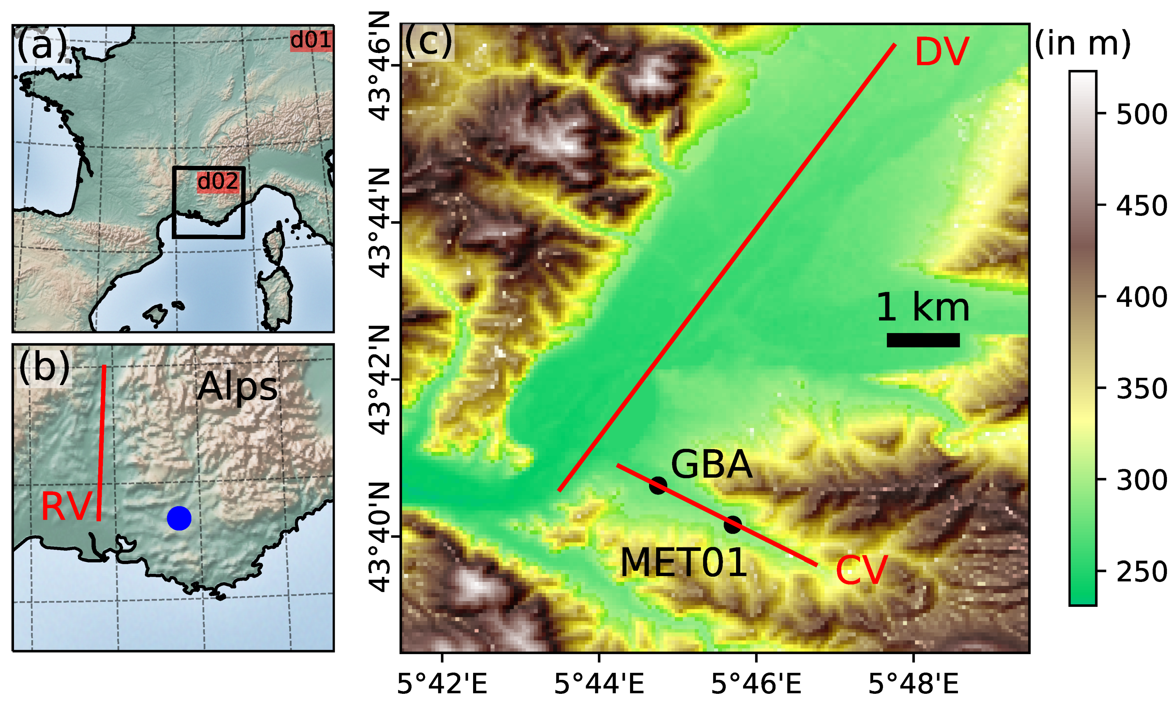
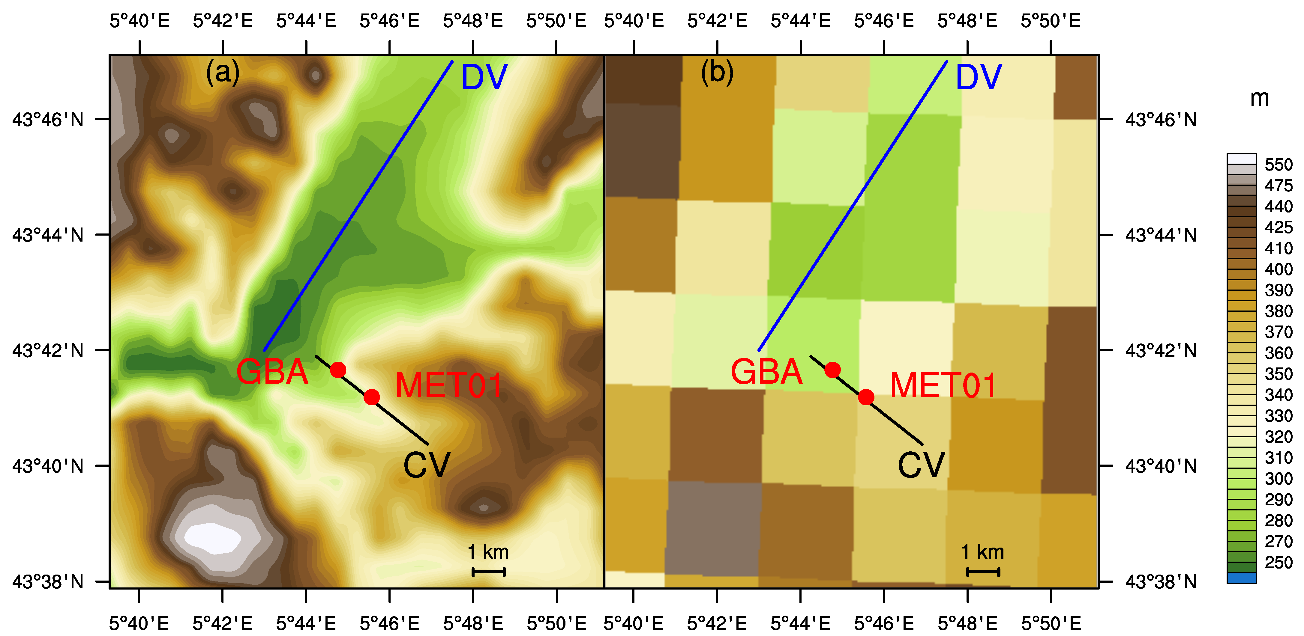
2.1. Topography and Land Use

The study area is located in the Alpine foothills of southeastern France, featuring many small valleys and hills (Figure 1). The Cadarache site mainly stretches along a small tributary valley of the larger Durance valley (DV). The latter coming from the northeast in an almost rectilinear segment approximately 67 km long, 200 m deep, 5 km wide with a mean slope of 0.2°. The Cadarache valley (CV) is oriented in a southeast to northwest downslope direction. It is approximately 6 km long, 100 m deep, 1–2 km wide, and has a mean slope of 1.2°. The red lines of Figure 1c indicate the axes of these perpendicular valleys. Valley floors are mostly farmland with sparse trees and scattered buildings whereas hillsides and ridges are covered by denser vegetation from shrubs to sclerophyllous forests.

2.2. Routine Local Measurements

This study uses hourly-averaged values of meteorological parameters continuously measured at the GBA and MET01 stations, both installed at the CV bottom (Figure 1c). The GBA tower is located at 265 m a.s.l. at the lower end of the CV, about 2 km upstream of the DV’s main axis. The MET01 location is 1.6 km up-valley of GBA and 286 m a.s.l, approximately at mid-length of the CV. The instruments at the two sites along with the corresponding period of available data are detailed in Table 1

2.3. Weather Conditions

The Cadarache site is at the edge of the Mediterranean climate and is influenced by its proximity to the Alps. Synoptic winds that interfere with low-level winds in the CV originate mostly from three main directions as evidenced by the wind rose observed at GBA 110 m above the valley floor (just above the Cadarache valley ridges) (Figure 2a).
First, the left lobe of the wind rose results from usual mid-latitude westerly winds and from the “Mistral”. The Mistral is normally a strong northern wind, channeled by the Rhone valley located in the west (see Figure 1b), which spreads out when it comes over the Mediterranean coastal plains and consequently takes on a northwesterly orientation when it reaches Cadarache [32]. Second, the “Marin” coming from the Mediterranean Sea blows from the southeast and is often associated with rain. Third, winds coming from the Alps in the northeastern quadrant are more or less channeled by the DV [10].
Additionally, when the sky is clear (which is frequently observed in this region), and synoptic conditions are calm, thermally driven winds take place in the Durance and Cadarache valleys. In daytime, anabatic winds occur as a consequence of horizontal temperature gradients resulting from the complex relief and the penetration of sea breeze from the 50 km distant Mediterranean coast. In contrast, radiative cooling at night promotes stable conditions and katabatic flows that have been extensively documented during the KASCADE 2013 campaign [10]. The reader is referred to Dupuy et al. [22] for a detailed description of these classic weather conditions over Cadarache.

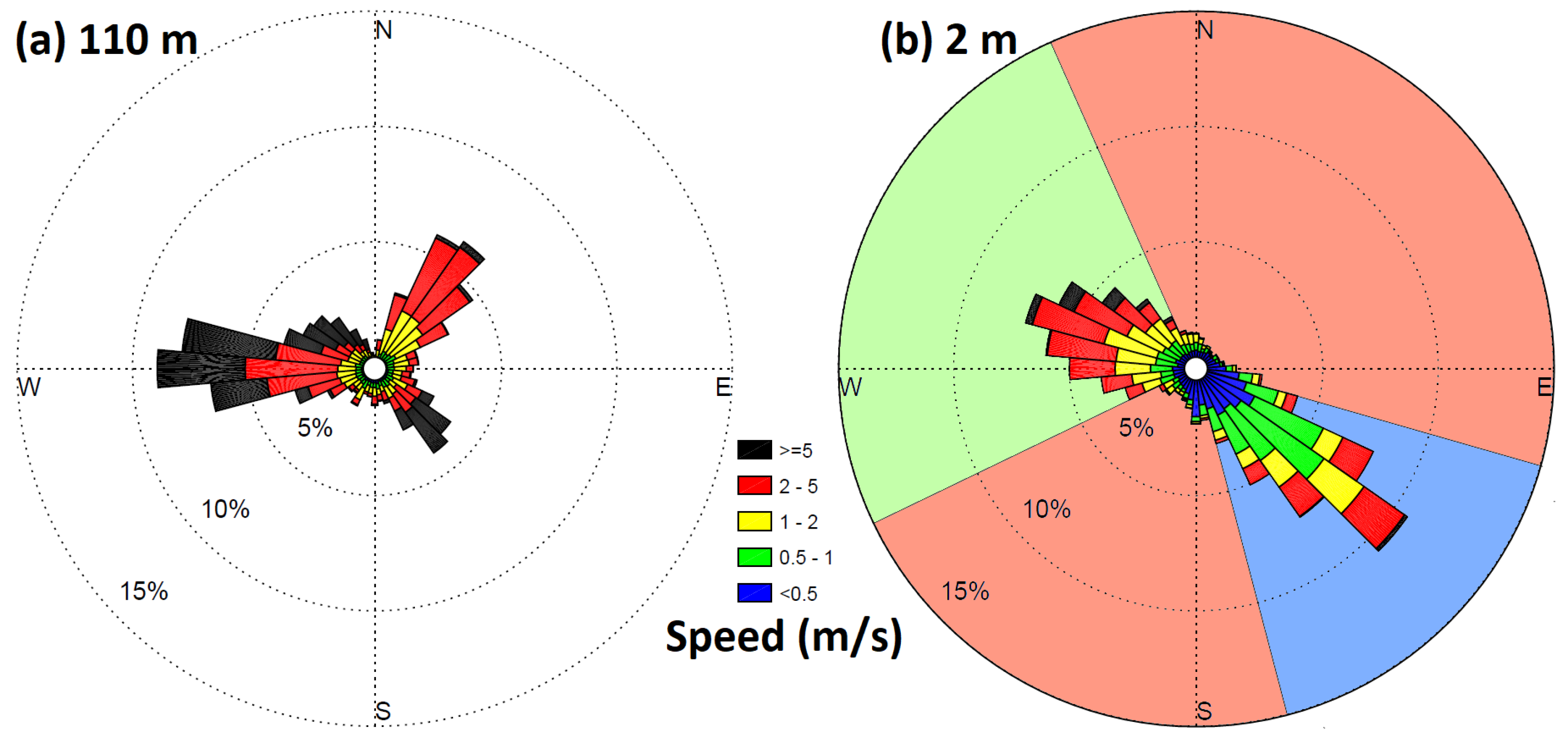
2.4. Cadarache Valley Wind

As illustrated in Figure 2b, the SE and NW wind directions dominate inside the CV. Down-valley winds are grouped in the blue sector (39% of observations, between 105° and 165°), and up-valley winds in the green one (also 39% between 245° and 335°). The red sector contains the remaining 22% cross valley winds, almost half of them having speeds lower than 0.5 m s−1.
The relationship between winds observed above (110 m a.g.l.) and inside (2 m a.g.l.) the CV, represented in Figure 3, highlights coupling/uncoupling conditions (cf. Whiteman and Doran [1] for a definition of those conditions). Coupled winds lie along the main diagonal with a high probability density for SE and W to NW directions. These result from downward momentum transport combined with channeling, according to the classification of Whiteman and Doran [1]. The other high-density spots reveal CV flows uncoupled from the wind aloft, most of them flowing down-valley (direction tagged CDV for Cadarache down-valley). This is particularly visible for calm conditions where the CDV wind coexists with the Durance down-valley (DDV) wind aloft.

3. Numerical Simulations

3.1. WRF Configuration

The tuning of the operational WRF model used by the CEA in Cadarache is the result of various tests [33,34] aiming to improve the ability of the model to simulate crucial parameters, such as the Diurnal Temperature Range (DTR) in the Cadarache valley. The configuration used in the present study (see Table 2) differs in two ways from the operational tuning. The GFS is used instead of the ERA-ECMWF as initial and boundary forcing due to regulatory constraints, and only two nested domains are kept because of computation time constraints.
Domain #1 covers France (Figure 1a) with a 9 km horizontal resolution. Domain #2 (Figure 1b), with a finer horizontal grid spacing of 3 km, is focused on the southeastern part of France. With a 3 km horizontal resolution, the most important geographical features impacting weather conditions over Cadarache (see Section 2.3) are resolved (e.g., Rhone and Durance valleys, the southern Alps and the Mediterranean coastal region), but the smaller Cadarache valley is not resolved (Figure 4).

3.2. Data Extraction

Based on preliminary tests and previous results [43,44], it appears that a good stabilization of the model is obtained after a spin-up time of half a day. For this study, in order to be sure to overpass the spin-up period, the [0, 23 h] lead time period is thus discarded. On the other side, considering that the forecast performance decreases as the lead time increases, we did not consider forecasts for times longer than two days. The lead times from 24 h to 47 h are thus kept from each daily simulation. This extraction process results in a continuous time series over 1 year from daily forecast runs with no overlapping.
In order to compare WRF forecasts to GBA and MET01 observations, WRF variables were extracted at these sites locations using a bilinear interpolation. The WRF profiles were then interpolated along the vertical to the heights of the observations. Only data from the domain #2 were used.

3.3. Forecast Evaluation

The goal of the study is to establish a reliable wind forecast in the Cadarache valley. Therefore, our forecast evaluation mainly focuses on wind. Nevertheless, being aware that stability is the main trigger of down-valley winds [31], the atmospheric stratification is evaluated as well.

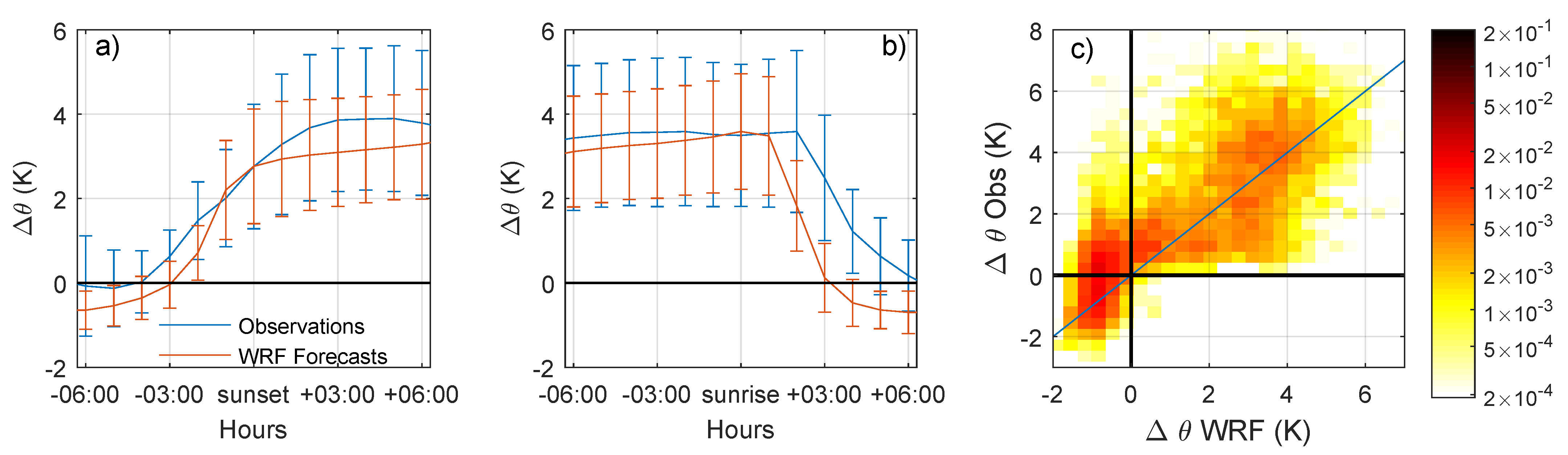
3.3.1. Atmospheric Stratification
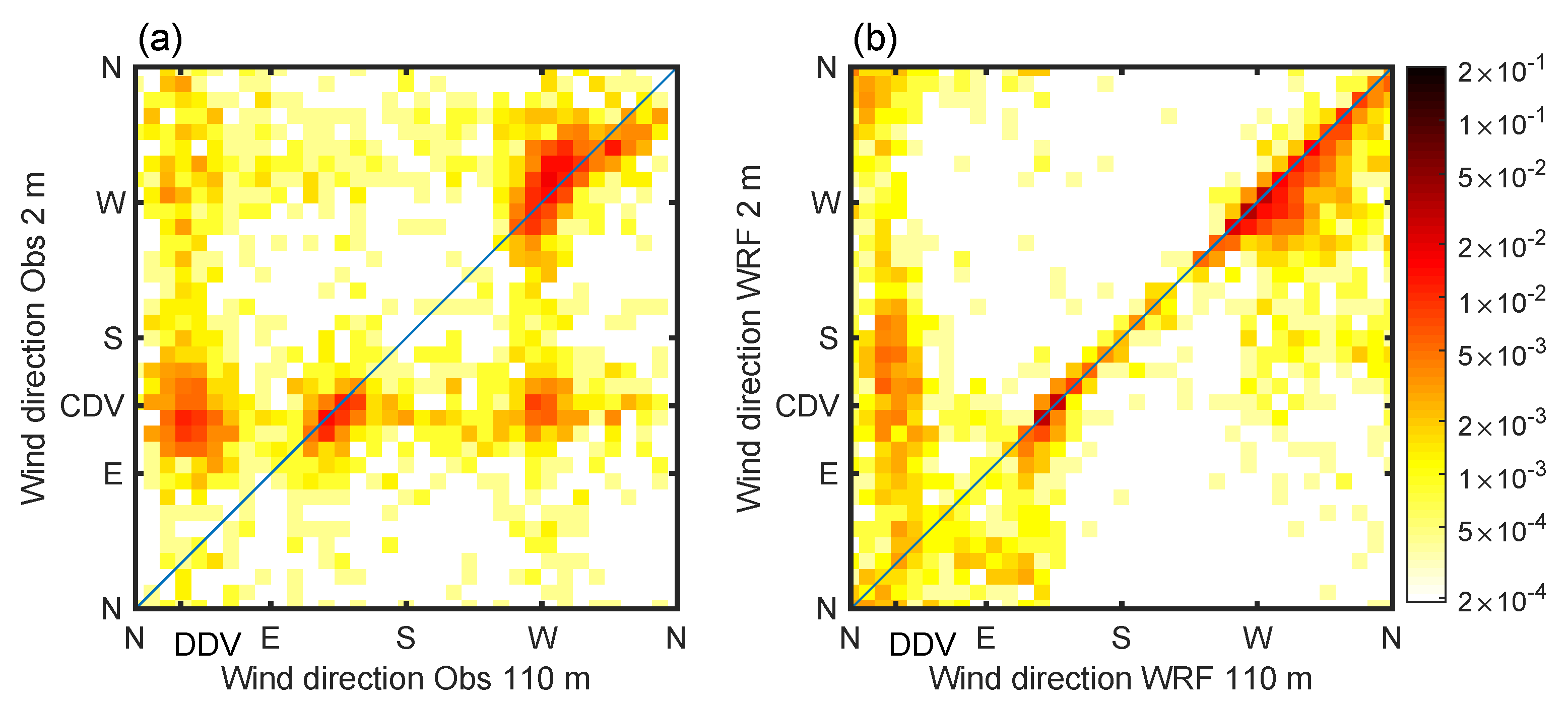
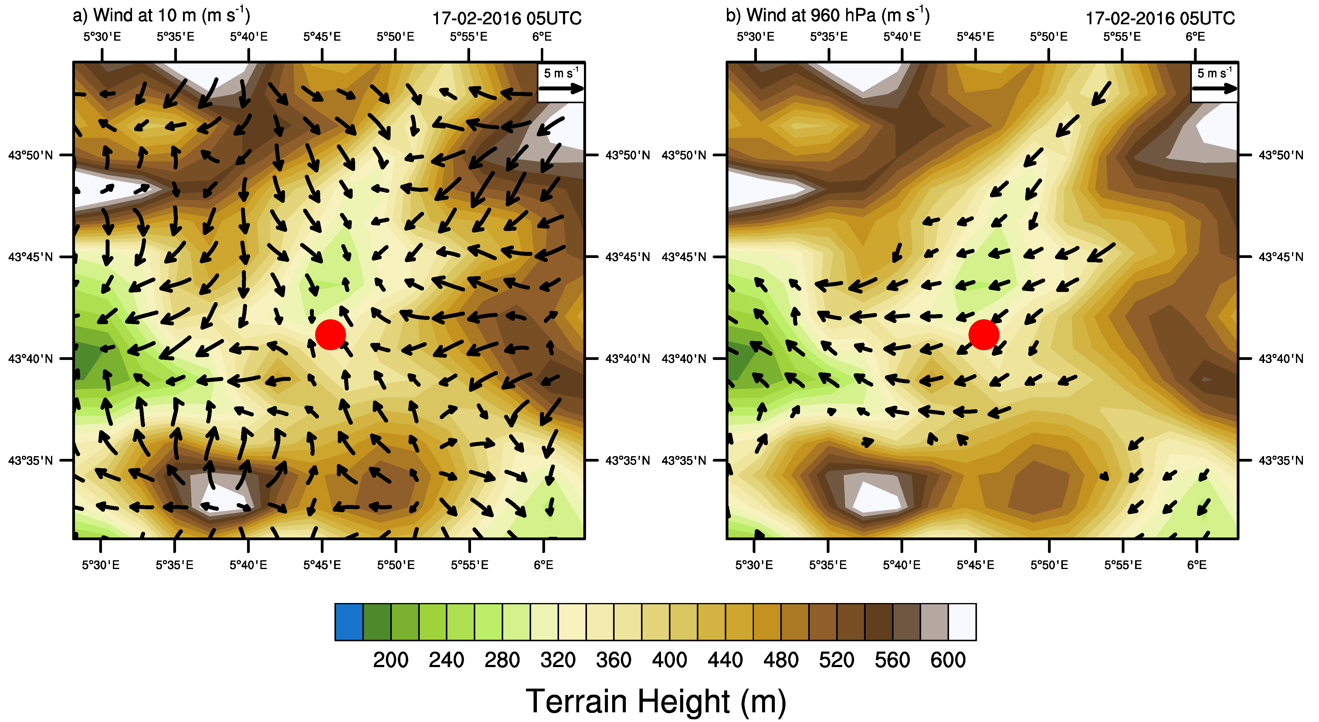
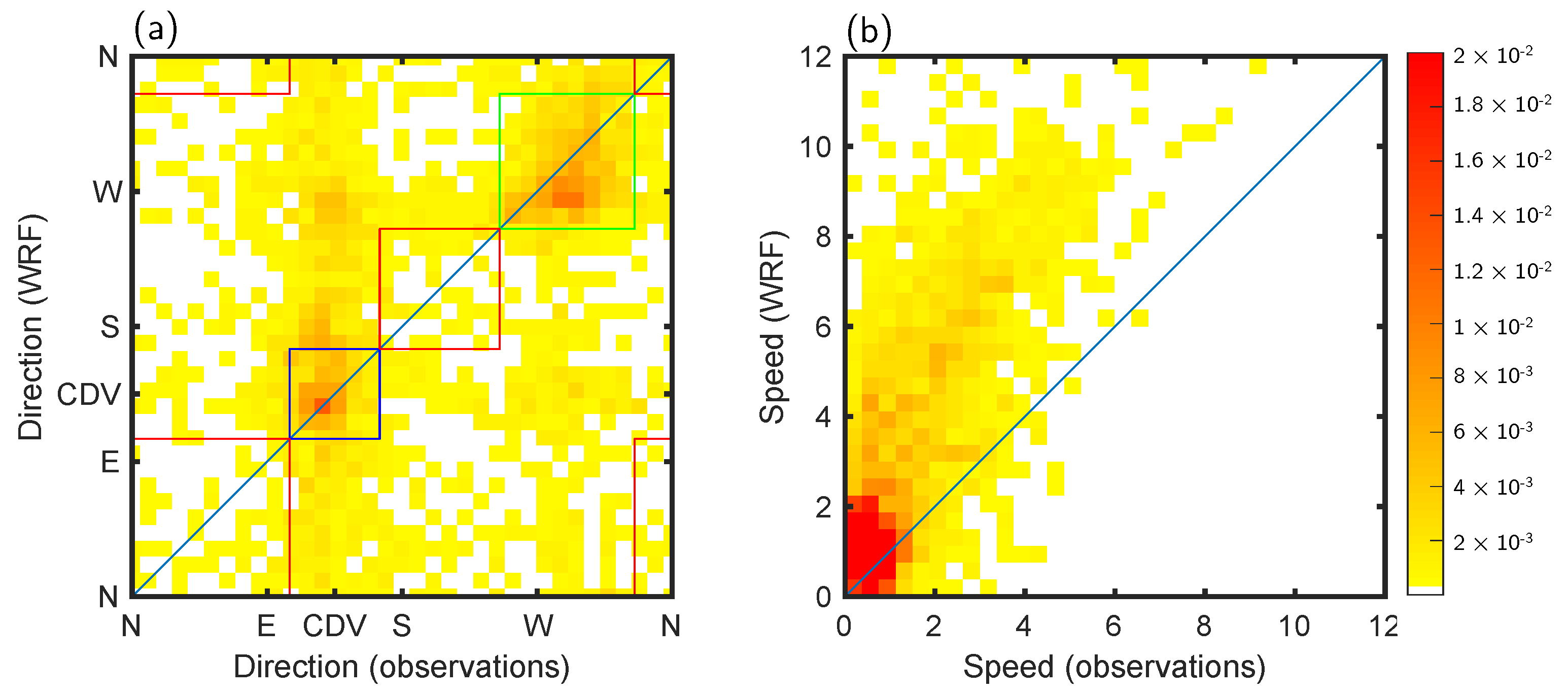
The forecast stratification is compared to GBA permanent measurements. Potential temperature at 110 m in observations was calculated assuming that pressure variation between 2 and 110 m obeys the dry hydrostatic law. A sensitivity study showed that it is a good approximation since the mean resulting uncertainty on potential temperature does not exceed 0.1 °C (see Appendix A in Dupuy [45]). Observations show that the daily cycle of Δθ (the vertical difference of potential temperature between 110 m and 2 m) is usually well marked: the atmosphere is stably stratified during the night and unstable during the day (Figure 5a,b). This cycle is overall well reproduced in the simulations except during morning and evening transitions. The transition to unstable conditions occurs around 3 h earlier in WRF, while transition to stable conditions occurs with a delay of around 1 h.
The probability density function graph (Figure 5c) shows the level of agreement between the observations and the simulations. It can be divided into three parts: The first one covers the observed negative Δθ (unstable stratification), corresponding to daytime periods. In this part, the simulated values are also negative and a large part of the values are grouped close to the 1:1 line which reflects a good agreement. The second part covers the observed values included in the range [0, 2 °C], which corresponds to the afternoon and evening transitions. There is a poor agreement in this range, with simulated values spread between −1 °C and 4 °C. The last part covers the observed values higher than 2 °C, which corresponds to stable nighttime periods. The simulated atmosphere is stably stratified too, but there is a large scatter showing the difficulty of accurately simulating the intensity of the stratification during the night.

3.3.2. Winds

Methodology

The comparison of wind forecasts is based on the metrics described in Dupuy et al. [22]. Wind direction forecast evaluation is based on (i) the DACC (Direction Accuracy [46]) metric, which represents the proportion of horizontal winds which do not depart by more than 45° from observations, and (ii) the PC (Proportion Correct) metric, which indicates the proportion of values correctly classified in different wind sectors defined from the observed wind rose to represent the main wind regimes. Two forms of PC are used. PC2 [31] considers two wind sectors: the southeast quarter for downvalley winds for the first class and all other directions for the second class. PC4 considers four classes: a first class for light winds (lower than 0.5 m s−1) that have no well-defined direction, a class of CDV winds, a class of upvalley winds, and a class of cross-valley winds. The last three classes correspond to the blue, green, and red regions, respectively, in Figure 2b. Wind speed forecasts are assessed using the Pearson correlation coefficient, bias, and mean absolute error (MAE). Forecasts are compared to observations at the MET01 station, where wind is measured with a Young 05103 anemometer with an accuracy of ±0.3 m s−1 and ±3° for the speed and direction.

Results

At MET01, we used the WRF 10 m wind output. In order to compare the simulated wind to the observations, wind speeds have to be extrapolated down to 2 m. To do that, we took advantage from the 3-month period of KASCADE [10] during which we have wind observations at these two levels. We found that a simple linear regression ( U 2 m = 0.82 × U 10 m 0.07 , where U 2 m and U 10 m are the wind speeds at 2 m and 10 m expressed in m s−1) satisfactorily extrapolates wind speeds from 10 m to 2 m, yielding even better results (mean absolute error of 0.12 m s−1) than assuming a logarithmic wind profile (mean absolute error of 0.61 m s−1) [45]. We assume that wind directions at 10 m and 2 m are identical.
The influence of above-valley winds on near-surface winds in the Cadarache valley is crucial (see Section 2). The relationship between these two winds in WRF highlights a major discrepancy with observations (Figure 6). While decoupling (i.e., wind directions considerably different between the two levels) occurs frequently in observations, especially under stable conditions leading to CDV winds at 2 m, it is underpredicted in WRF. This is particularly striking for CDV 2 m winds associated with 110 m winds coming from the West (usually occurring early in the night, before the appearance of the northeasterly DDV 110 m wind). Another significant difference between observations and simulations corresponds to decoupling situations when 110 m winds are blowing down the Durance valley (DDV). In such conditions, the associated observed 2 m winds cluster around the CDV direction, whereas simulated 2 m wind directions are much more scattered. It appears that the low-level wind in the model is constrained by the coarse representation of the local topography. We give an illustration of this behavior with the situation on 17 February 2016 at 05UTC (Figure 7). At 960 hPa, a level corresponding approximately to 110 m above the ground (the ground level pressure at MET01 was 973 hPa at this time), the simulated winds are blowing down the Durance valley (which corresponds well to the observations), whereas surface winds are blowing along the resolved slopes, alternatively yielding northeasterly to south-southwesterly winds at the MET01 site.
Simulated surface winds are therefore less channeled than observations. This is illustrated in Figure 8a, especially for the down-valley direction (SE): 39% of the observations lie in the 105°–165° range (corresponding to the blue sector on Figure 2b) versus 23% in the simulations. Simulated wind speed has a positive bias of +1.07 m s−1 (Figure 8b), which is a consequence of the misrepresentation of subgrid topography in WRF. The metrics calculated on the WRF 2 m winds are summarized in Table 3. Only 50% of wind directions are forecasted with an error lower than 45° (DACC), and only 47% are well classified considering 4 classes (PC4).

4. Artificial Neural Network

An ANN is a statistical tool that is able to correlate complex data inputs. The ANN learns to perform tasks by considering examples, generally without being programmed with any task-specific rules. In this study, the task consists of reproducing the winds observed at the bottom of the Cadarache valley (described in Section 2.4), starting from WRF output variables. In other words, the objective is to find the mathematical function linking coarsely modeled WRF-forecast variables to highly localized near-surface wind observations.
An ANN function is composed of neurons (a linear combination of input variables transformed by a so-called activation function) interconnected between each other and arranged in layers. The ANN starts with a pseudo-randomly chosen function (pseudo-random setting of initial linear combinations weights). Then, the training step consists of fitting the function (that is to say the weights) to produce results as close as possible to the ground truth. Weights are iteratively updated, based on results calculated on a subset of the dataset (called training set), until the performance (the loss function), calculated on a second subset of the dataset (called validation set), reaches a given limit and no longer improves. A third subset, called test set, is used to calculate metrics and compare results between different ANNs. The three subsets are totally independent and, in order to calculate unbiased metrics, the test set is not used during the training step.
As ANNs are good interpolators but poor extrapolators [21], the dataset used to train the ANN has to include numerous and heterogeneous examples to encompass the widest range of cases that the ANN is expected to treat.

4.1. ANN Configuration

The configuration of the ANN used in this study is similar to that described in [22]. It is a multilayer perceptron (MLP) type [47], which is frequently used in atmospheric sciences [21]. Its specific feature is that each neuron of a layer is connected with all neurons of the previous and next layers. It is composed of an input layer, at least one hidden layer and an output layer. Here, the input layer simply consists of the WRF variables. There is a single hidden layer of 10 neurons. To support this choice, we verified that the performances were not improved by adding a second hidden layer, and we evaluated the evolution of the ANN performance when the number of neurons in the hidden layer varied from 5 to 50. The output layer is composed of two neurons that are expected to reproduce the horizontal wind components at 2 m (i.e., u and v). These components are used to calculate wind speed and direction. The activation function is a hyperbolic tangent function because it offers more favorable results than other tested functions (e.g., logsigmoid or linear functions). The ANN was conducted using MATLAB’s Deep Learning Toolbox. The Levenberg–Marquardt algorithm was chosen as the training algorithm because it is described in the MATLAB toolbox user’s guide as the fastest training algorithm while offering performances very similar to all other tested algorithms, such as BFGS Quasi-Newton, and Scaled Conjugate Gradient. The pseudo-random generation of the initial weights is also tested by training several ANNs with different seeds. The seed producing the best results is selected.
The dataset was randomly split into 60% training data, 10% validation data, and the remaining 30% was used as the test subset. Random split guarantees that each of the 3 subsets contain data from all the different meteorological seasons. We did not run the ANN on seasonal subset data because we consider that ANN would better work when the training and validation data set encompass the widest possible meteorological conditions. The risk for a subset of data restricted to specific conditions is that the ANN output would possibly fail when an odd situation occurs (for example, a quite warm day in winter, or easterly wind in spring). Input variables and ground truth were normalized between −1 and +1 in order to avoid weight discrepancy problems, which occur when the order of magnitude of variables differs.

4.2. Selection of Input Variables

Based on the recommendations of Dreyfus et al. [48], the most pertinent variables to use as input to the ANN are selected following a two-stage process.
First, a selection removes redundant WRF variables. Meteorological variables such as temperature, atmospheric pressure and humidity are interrelated, and therefore they share a part of the information they carry (for example, the diurnal cycle). When the absolute value of the correlation coefficient between two variables is higher than 0.9, they are considered redundant and one of them is removed from the ANN input dataset. This step is called hereafter “filter selection”.
Second, an iterative process called sequential forward selection [49] is performed. A reference ANN (called ANNref) is launched with all variables still remaining as inputs after the filter selection. For the first iteration, “elementary” ANNs are trained, each one using a single input variable taken among the input variables of ANNref. The metrics of these elementary ANNs are compared to each other and the variable giving the best results is selected for the next step. The input variable set is thus progressively constructed by adding the best variable to the selected variables at each iteration. The performance of the ANNs is compared to the reference one at the end of each iteration. This process is continued until improvements in the performance metrics are no longer significant.

4.3. Significance of Results

A bootstrap method was applied to assess the significance of metrics scores. Ten thousand test subsamples were created from the original test set, using a random draw with replacement. The ANN function is then applied to each subsample, producing 10,000 output datasets. The metrics are calculated for each output dataset leading to a distribution for each metric. This distribution is used to calculate the mean value for each metric with a confidence interval (at 90%) defined as the interval between the 5th and 95th percentiles.

5. Results and Discussion

5.1. Selection of Input Variables

Output variables from WRF daily weather forecasts are used as inputs for the ANN. An empirical selection among the numerous WRF output variables was performed prior to the selection steps described in Section 4.2. This empirical selection was based on knowledge of the local meteorology in the Cadarache valley (see in [10] and Section 2), and a previous application of ANNs to nowcast local wind in the Cadarache valley [22].
Specific conditions leading to different near-surface/above-valley winds relationships, described in Section 2, depend mostly on wind speed and direction as well as stratification. Thus, wind speeds and components at three heights (10, 110, and 300 m) above the ground were tested as inputs. We chose the 300 m level winds because it is the level of maximum intensity of the nocturnal Durance downvalley jet [10], 110 m because it is the height corresponding to the wind measurements at GBA, and 10 m because it is the lowest level in the model. Moreover, physics-guided neural networks, which provide a framework for combining scientific knowledge of physics-based models with ANN [50,51], suggest adding the modeled variable to be corrected as an input variable (10 m wind components in our case). The profile of the potential temperature θ characterizes the vertical stratification. Previous studies [22,31] have shown that a valley-scale (the valley is around 100 m deep) stratification intensity based on a vertical difference of the potential temperature between 110 m and 2 m (Δθ) was crucial in nowcasting winds in the valley. We thus decided to use the same variable calculated from the simulations. Other stability-related variables were selected: a bulk Richardson number (in the layer 110 m–2 m), the friction velocity and the atmospheric boundary-layer height (defined as the level at which the kinetic turbulent energy becomes lower than 0.01 m2 s−2, according to the work in [52]). The net radiation at the surface was also added as it provides information on the thermal forcing.
In addition, even knowing that the CDV wind onsets and disappearances are not exactly reproducible through days, Duine et al. [10] showed that it generally appears around sunset and disappears approximately 2 h after sunrise (consistent with Figure 5). Moreover, Dupuy et al. [22] showed the considerable information brought by the diurnal cycle in order to nowcast the CDV wind. For this reason, we added the time relative to the closest sunrise and sunset time, respectively.
Finally, common meteorological parameters were also added: potential temperature at 2 and 110 m, atmospheric pressure, specific humidity at 2 m, surface temperature and rainfall.
The Dreyfus et al. [48] two-step selection was then applied to the previous list of variables. Strong correlations (R > 0.9) were found for some couples of variables. Potential temperature at 2 m was discarded because it is strongly correlated to both surface temperature and 110-m potential temperature. Surface temperature was also discarded because it has high correlations with several other variables (the atmospheric boundary-layer height, the vertical difference of potential temperature, the friction velocity, and the net radiation at the surface). The 110 m wind (u and v components and speed) is highly correlated with winds at 10 and 300 m, resulting from the smoothed topography in WRF. This is consistent with WRF’s overly strong coupling between winds 10 and 110 m, as shown in Section 3.3.2. On the other hand, winds at 10 m and 300 m are less correlated, which justifying retaining these variables (u and v components and horizontal speed magnitude) at both levels. Finally, the friction velocity was discarded because it is highly correlated to the wind speed at 10 m as well as with the boundary-layer height.
After this first selection process, 16 variables were left. Then, the sequential forward selection produced a dataset of five variables: Δθ, wind components at 10 m, net radiation, and specific humidity at 2 m. These five variables are used as inputs to the ANN, the results of which are presented below.

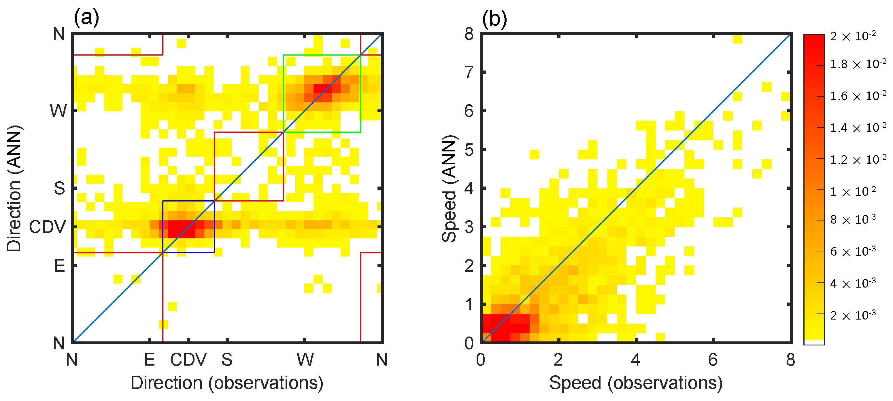
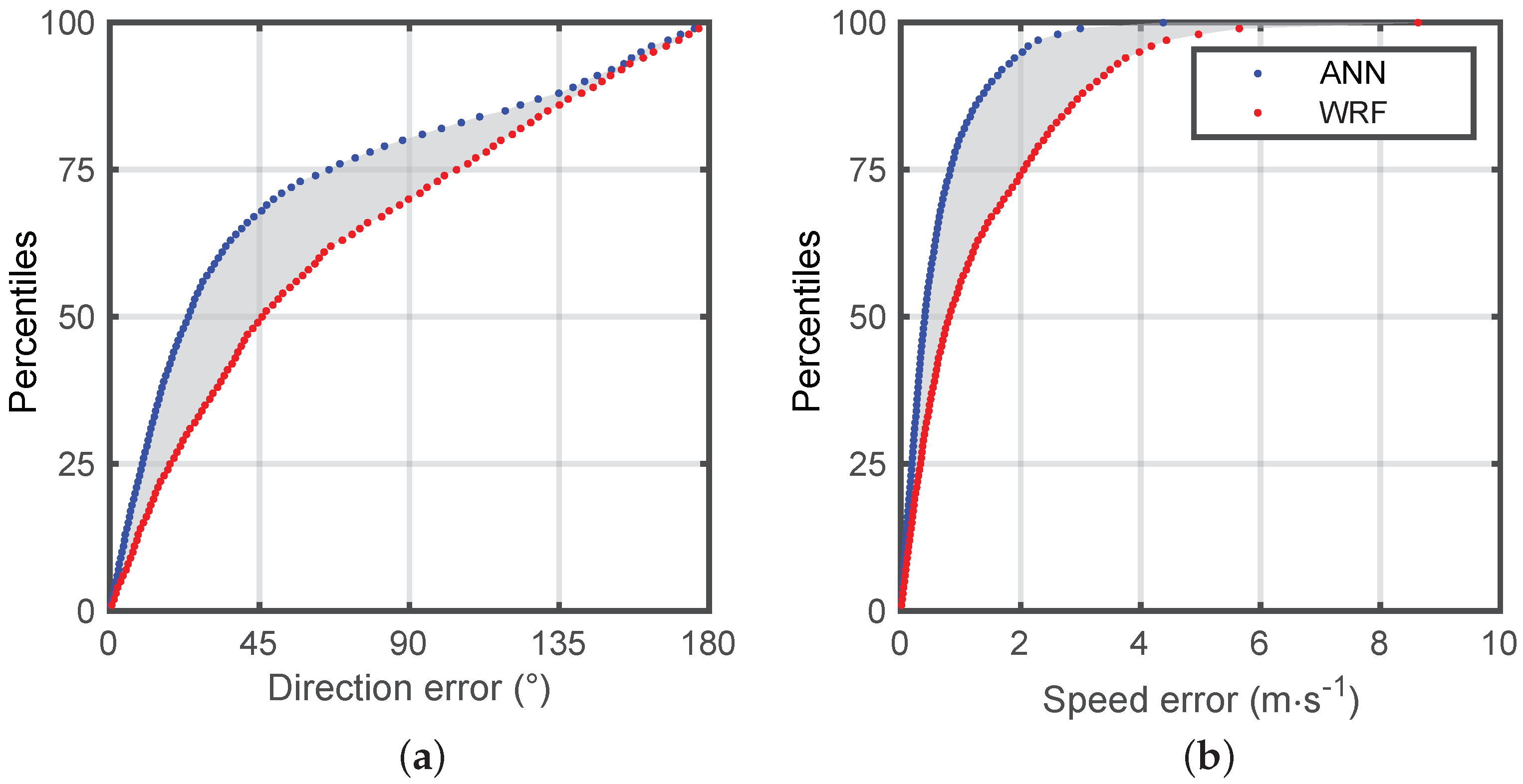
5.2. ANN-Related Forecasting Improvements

Figure 9 presents a comparison between wind observations at MET01 and the corrected winds resulting from the ANN applied to WRF forecasts. Referring to Figure 8, where a similar comparison was done but for the “raw” WRF forecasts, we note the corrected ANN winds are significantly better. The data (direction and speed) now cluster around the 1:1 line. The improvement is quantified by the metrics given in Table 4. All the metrics improve significantly after the ANN processing. The ANN lowers the WRF positive wind speed bias, from +1.07 m s−1 for WRF to −0.34 m s−1 for the ANN, which is within the overall accuracy of weather station standard anemometers. Likewise, there is an improvement in the direction forecast with a better representation of along-valley oriented winds (higher concentration of data in the blue and green squares with the ANN in Figure 9), which is confirmed by the improvement of DACC (from 0.50 to 0.68) and PC4 (from 0.47 to 0.71) values.
Figure 10 represents another way to visualize the gains achieved with the ANN using the cumulative distributions of errors for wind speed and direction. The gray area represents the gain resulting from the ANN. For example, the percentage of wind direction errors less than 20° represents 27% of the dataset for WRF forecasts versus 46% for the ANN. We note that the percentile values for the 45° error corresponds to the DACC reported in Table 4.
Two regions are identified in the cumulative distribution of direction errors. For errors higher than 135° corresponding to forecast directions quite opposite to the observations, the differences between the two distributions are small. That means that the ANN is not able to significantly improve the worst direction forecasts. Differences occur for errors in wind direction lower than 135°, and particularly for the lowest errors: about half of the WRF forecasts have an error lower than 45°, whereas this amounts close to 70% for ANN data. That means that the ANN corrects a part of intermediate errors. More details on that are given in Section 5.3.2.
Likewise for the speed, the 75th percentile value corresponds to an error of 2.05 m s−1 for WRF forecasts versus 0.83 m s−1 for the ANN. This means that 75% of ANN outputs have errors lower than 0.83 m s−1 (2.05 m s−1 for WRF forecasts). These results visually confirm the decrease of MAE (0.62 m s−1 for the ANN and 1.32 m s−1 for WRF).

5.3. ANN Strengths and Weaknesses

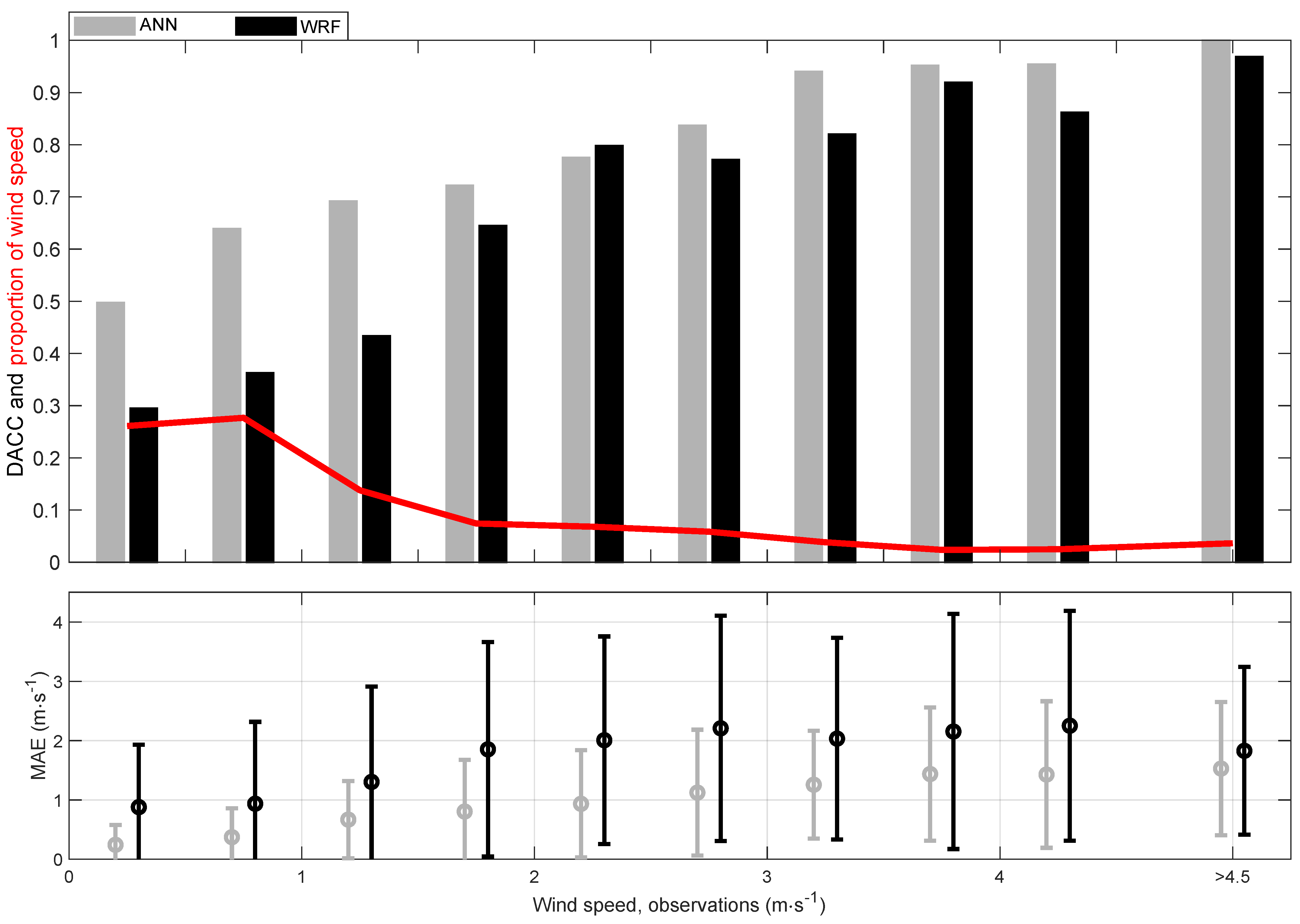
5.3.1. Influence of the Wind Speed

The evolution of ANN performances with wind speed is represented in Figure 11. The performance of WRF’s wind direction forecast improves with stronger wind speeds, which is consistent with results of Jiménez and Dudhia [53]. As shown is Section 2, strong above-valley winds are more efficient at forcing low-level winds, leading to relatively small wind direction rotations with the height. Corresponding low-level wind directions are thus less dependent on the valley topography, which explains the good behavior of WRF forecasts. On the contrary, the MAE of WRF wind speed prediction increases with the strengthening of winds (at least until 3 m s−1).
The ANN improves the forecast of both the speed and direction regardless of the wind speed magnitude. Wind direction improvements are more evident for light winds, which is fortunate because they represent a high proportion of the dataset. This probably results from a smaller progress margin for the strongest winds (DACC higher than 0.8 for winds stronger than 3 m s−1 for WRF). Regardless, ANN performance is better even for strongest winds. Concerning speeds, the ANN diminishes the MAE and the standard deviation irrespective of wind speed.

5.3.2. Light Winds and Channeling

Two weaknesses emerged when applying ANNs to the WRF wind forecasts, similarly to what was already mentioned by Dupuy et al. [22] in their nowcasting approach.
First, as already mentioned above, the ANN encounters some difficulties in correctly reproducing light wind directions. These defects are attributed to the method used to calculate the direction, which is not directly an ANN output, but is derived from the wind components (which was already discussed in Dupuy et al. [22]). For light winds, the wind components are small. A small absolute error made on one of the components produces large errors on the direction. On the other hand, the same small error in one of the components associated with a strong wind has a relatively smaller impact on the direction, producing a smaller error.
Second, there are differences in observed and ANN distributions of direction, since the ANN mainly produces valley-oriented winds, failing to reproduce most of cross-valley winds. Figure 9 clearly shows the strong channeling of winds along the valley axis, with very few northeasterly and southwesterly wind observations. Light speeds, a lack of typical meteorological conditions (unlike up- and down-valley winds) and fewer observations of these winds explain the weakness.

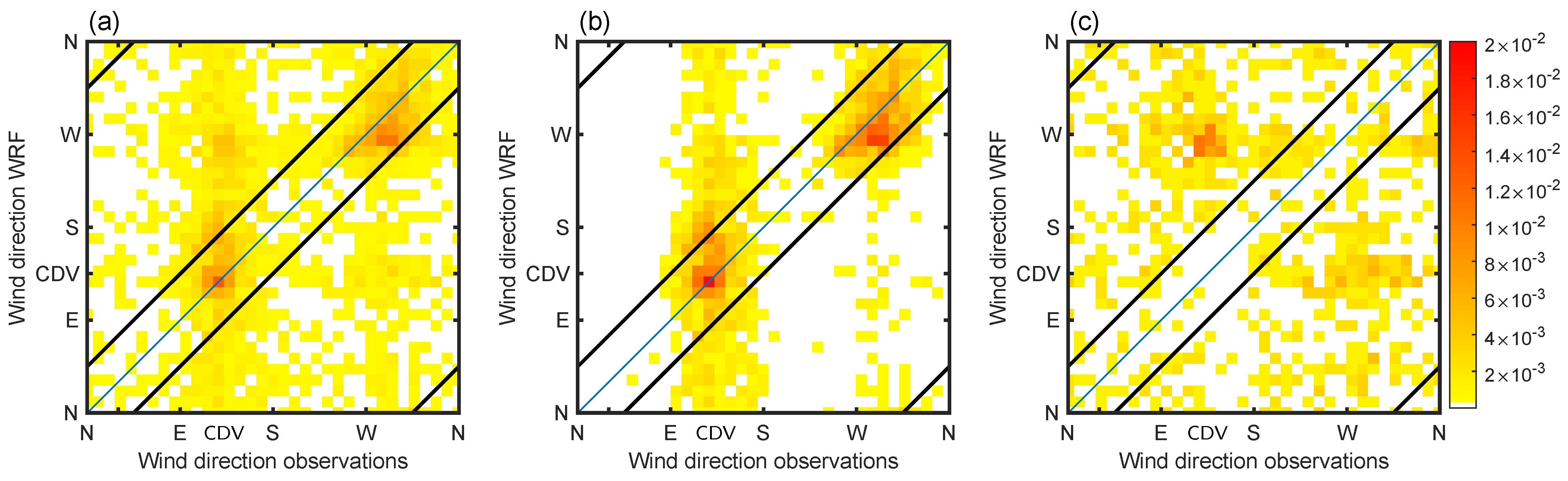
5.3.3. Improvement of Valley Winds Prediction

In order to visualize the improvements/degradations brought about by the ANN with respect to the raw WRF forecasts, we split the data set into two parts, namely, “good” and “bad” ANN results. “Good” means that the ANN-calculated wind direction does not depart by more than 45° from the observed direction, and “bad” is all other cases. The results are presented in Figure 12. Figure 12b shows a comparison between WRF and observed directions for good ANN results. The data located between the two central black tilted lines or in the upper-left and bottom-right corners thus correspond to simultaneous good WRF and ANN direction forecasts, while the other areas correspond to bad WRF-forecasts and good ANN-forecasts (improvement using the ANN). The same comparison for bad ANN forecasts is plotted in Figure 12c, meaning that data located between the two central black tilted lines and in the up-left and bottom-right corners correspond to good WRF forecasts and bad ANN forecasts (degradation brought by the ANN).
For good WRF forecasts (50% of the dataset), the ANN keeps a good forecast for 89% of the cases (Figure 12b). The remaining 11% are mainly cross-valley winds, which are difficult to forecast with the ANN (see Section 5.3.2). Concerning bad WRF forecasts (Figure 12c), 47% are corrected by the ANN. They correspond in particular to southeasterly winds, which present the worst forecast performance in WRF (cf. Section 3). The conditions for which the ANN is not able to correct wind directions mainly correspond to directions opposite to the observations and aligned along the valley. These results are consistent with the cumulative distribution of direction errors (Figure 10a).

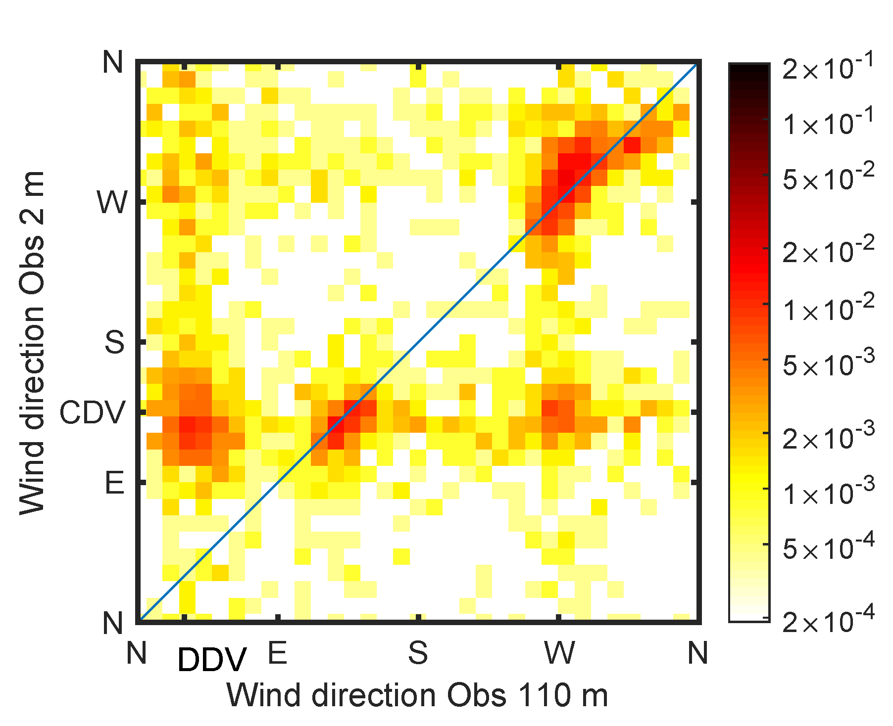
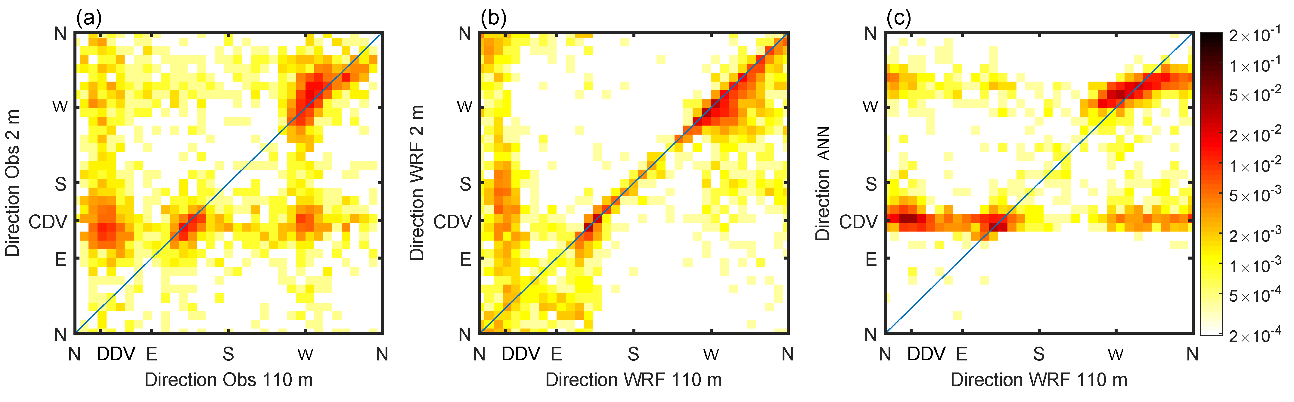
5.3.4. Relationship Between above and Inside Valley Winds

It was demonstrated in Section 3.3.2 that winds inside and above the Cadarache valley experience different relationships (coupled or uncoupled). The ANN is able to improve the representation of the complexity of that relationship in comparison with WRF forecasts alone (Figure 13). While WRF over predicts coupled situations, the ANN is able to integrate the uncoupled situations. More generally, the ANN reproduces the different observed relationships: CDV wind in the valley can be associated with above valley winds coming from either SE (forcing), WNW or NE (DDV wind), whereas northwesterly winds (i.e., upvalley) in the Cadarache valley can be associated with above valley winds coming from either NE (DDV winds) or NW (forcing). The improvement is particularly striking for CDV winds associated with northwesterly winds above it, often corresponding to early night uncoupled situations, which were never forecasted by WRF, and that the ANN is able to reproduce.

6. Conclusions

The aim of this study was to complement WRF operational mesoscale simulations (with a 3 km horizontal resolution) in order to predict a local wind mostly forced by subgrid-scale orographic effects.
The area of study is the Cadarache valley, which is 1–2 km wide, 100 m deep, and 6 km long, with a main axis oriented 135°–315°. During stable conditions a decorrelation between above-valley and near-surface winds has been observed that result from thermally driven winds with directions forced by the topography.
Considering one year of continuous observation made at the Cadarache valley site (wind and temperature at 110 m, i.e., just above the depth of the valley, as well as wind and temperature at 2 m on the valley floor), the overall performance of the WRF simulations was first evaluated. Unsurprisingly, the wind at 2 m was not well forecasted due to the smoothing of local topography in the simulations. On the other hand, the wind at 110 m and the temperature difference between 110 m and 2 m are well forecasted, showing that some parameters, poorly related to the local unresolved topography, can be well reproduced even with a coarse horizontal resolution. We thus started from the ideas developed by Dupuy et al. [22], who showed that these parameters could be used to feed an ANN in order to nowcast the wind at the bottom of the valley.
The ANN technique was applied to WRF operational forecasts outputs. For every day of the full year during which the observations were available, the 24-to-47 h forecast period was used to calculate the horizontal wind components observed at the bottom of the valley. One year of data was used, which constitutes a large enough dataset to encompass most of the meteorological conditions that are representative of the Cadarache site.
The selection of the WRF variables used to feed the ANN was performed according to the two-step method of Dreyfus et al. [48]. After the elimination of redundant parameters, as well as parameters whose impact on the results were weak, five of them were retained (the low-level wind components, the difference in potential temperature between 110 m and 2 m, and the net radiation at the surface and the specific humidity at 2 m).
The ANN significantly improved the forecast of the wind in the Cadarache valley, for both speed and direction. The scores obtained for the full year reached 0.68 for DACC, 0.71 for PC4, the bias on wind speed was reduced down to −0.34 m s−1 and the MAE to 0.62 m s−1. The ANN rectified about half of the situations for which WRF failed in forecasting the low-level wind direction. The ANN has thus addressed the main failure observed in the WRF simulations concerning the valley winds: the wind direction is now satisfactorily forecasted and the wind speed bias is considerably decreased. The ANN performance improves as speed increases. This is probably related to the fact that the ANN output is not the direction itself (against which the performance is evaluated), but the two wind components, from which the direction is computed. A limitation encountered with the ANN method is the excessive forecast of valley-aligned winds, which is explained by the fact that most wind directions away from the valley axis correspond to very light winds whose directions are challenging to measure and for the ANN to reproduce.
A comparison of ANN outputs to very high resolution simulations (horizontal resolution around 100 m in order to have a good representation of the Cadarach valley) on some specific events (operational forecasts at 100 m horizontal resolution remains not possible due to computational time) would certainly help better understand strengths and limitations of the ANN.
In conclusion, bearing in mind the limitations mentioned above, the artificial neural network technique is a valuable tool for improving numerical simulations and forecasting local flows at a scale which is not resolved by the model. A set of observations large enough to encompass the variability of the meteorological conditions observed at a given location is required for the training step of the ANN used. As the ANN is a poor extrapolator, one year of data is a minimum size needed to encompass as many conditions as possible occurring in the different seasons. The ANN technique can therefore be used to estimate local flows from an operational weather forecast model the resolution of which is too coarse to take into account the local influence of the topography or land use. This promising technique might in the future be widely used in routinely forecasted meteorological fields, taking advantage from its high potential for the local improvement of weather forecasts as well as air quality questions. It constitutes a quite inexpensive technique to refine coarse forecasts output at specific location, while coping with the “gray zone” problem arising when refining the horizontal resolution down to (sub) kilometer scales.

Author Contributions

Conceptualization, all; methodology, F.D.; software, F.D.; formal analysis, F.D.; investigation, F.D.; resources, T.H.; writing—original draft preparation, F.D., P.D., T.H., and P.R.; writing—review and editing, all; visualization, F.D. All authors have read and agreed to the published version of the manuscript.

Funding

This work was funded by the MRISQ project at the CEA.

Conflicts of Interest

The authors declare no conflict of interest.

Abbreviations

The following abbreviations are used in this manuscript:
ANNArtificial neural network
CEACommissariat à l’Énergie Nucléaire et aux Énergies Alternatives
CDVCadarache downvalley
CVCadarache valley
DACCDirectional accuracy
DDVDurance downvalley
DTRDiurnal Temperature Range
DVDurance valley
KASCADEKatabatic winds and Stability over CAdarache for Dispersion of Effluents
LESLarge eddy simulation
MAEMean absolute error
MSEMeans squared error
PCProportion correct
WRFWeather research and forecasting

References

  1. Whiteman, C.D.; Doran, J.C. The Relationship between Overlying Synoptic-Scale Flows and Winds within a Valley. J. Appl. Meteorol. 1993, 32, 1669–1682. [Google Scholar] [CrossRef] [Green Version]
  2. Clements, W.E.; Archuleta, J.A.; Hoard, D.E. Mean Structure of the Nocturnal Drainage Flow in a Deep Valley. J. Appl. Meteorol. 1989, 28, 457–462. [Google Scholar] [CrossRef] [Green Version]
  3. Doran, J.C.; Fast, J.D.; Horel, J. The VTMX 2000 Campaign. Bull. Am. Meteorol. Soc. 2002, 83, 537–554. [Google Scholar] [CrossRef]
  4. Weigel, A.P.; Rotach, M.W. Flow structure and turbulence characteristics of the daytime atmosphere in a steep and narrow Alpine valley. Q. J. R. Meteorol. Soc. 2004, 130, 2605–2627. [Google Scholar] [CrossRef]
  5. Whiteman, C.D.; Muschinski, A.; Zhong, S.; Fritts, D.; Hoch, S.W.; Hahnenberger, M.; Yao, W.; Hohreiter, V.; Behn, M.; Cheon, Y.; et al. Metcrax 2006: Meteorological Experiments in Arizona’s Meteor Crater. Bull. Am. Meteorol. Soc. 2008, 89, 1665–1680. [Google Scholar] [CrossRef] [Green Version]
  6. Price, J.D.; Vosper, S.; Brown, A.; Ross, A.; Clark, P.; Davies, F.; Horlacher, V.; Claxton, B.; McGregor, J.R.; Hoare, J.S.; et al. COLPEX: Field and Numerical Studies over a Region of Small Hills. Bull. Am. Meteorol. Soc. 2011, 92, 1636–1650. [Google Scholar] [CrossRef] [Green Version]
  7. Fernando, H.J.S.; Pardyjak, E.R.; Di Sabatino, S.; Chow, F.K.; De Wekker, S.F.J.; Hoch, S.W.; Hacker, J.; Pace, J.C.; Pratt, T.; Pu, Z.; et al. The MATERHORN: Unraveling the Intricacies of Mountain Weather. Bull. Am. Meteorol. Soc. 2015, 96, 1945–1967. [Google Scholar] [CrossRef]
  8. Fernando, H.J.S.; Mann, J.; Palma, J.M.L.M.; Lundquist, J.K.; Barthelmie, R.J.; Belo-Pereira, M.; Brown, W.O.J.; Chow, F.K.; Gerz, T.; Hocut, C.M.; et al. The Perdigão: Peering into Microscale Details of Mountain Winds. Bull. Am. Meteorol. Soc. 2019, 100, 799–819. [Google Scholar] [CrossRef]
  9. Paci, A.; Staquet, C.; Allard, J.; Barral, H.; Canut, G.; Cohard, J.M.; Jaffrezo, J.L.; Martinet, P.; Sabatier, T.; Troude, F.; et al. The Passy-2015 field experiment: Atmospheric dynamics and air quality. Pollut. Atmos. 2017, 231–232. [Google Scholar] [CrossRef]
  10. Duine, G.J.; Hedde, T.; Roubin, P.; Durand, P.; Lothon, M.; Lohou, F.; Augustin, P.; Fourmentin, M. Characterization of valley flows within two confluent valleys under stable conditions: Observations from the KASCADE field experiment. Q. J. R. Meteorol. Soc. 2017, 143, 1886–1902. [Google Scholar] [CrossRef] [Green Version]
  11. Zhou, B.; Simon, J.S.; Chow, F.K. The Convective Boundary Layer in the Terra Incognita. J. Atmos. Sci. 2014, 71, 2545–2563. [Google Scholar] [CrossRef]
  12. Wagner, J.S.; Gohm, A.; Rotach, M.W. The Impact of Horizontal Model Grid Resolution on the Boundary Layer Structure over an Idealized Valley. Mon. Weather Rev. 2014, 142, 3446–3465. [Google Scholar] [CrossRef]
  13. Jiménez, M.A.; Cuxart, J. A study of the nocturnal flows generated in the north side of the Pyrenees. Atmos. Res. 2014, 145–146, 244–254. [Google Scholar] [CrossRef] [Green Version]
  14. Udina, M.; Soler, M.R.; Sol, O. A Modeling Study of a Trapped Lee-Wave Event over the Pyrénées. Mon. Weather Rev. 2017, 145, 75–96. [Google Scholar] [CrossRef]
  15. Conangla, L.; Cuxart, J.; Jiménez, M.A.; Martínez-Villagrasa, D.; Miró, J.R.; Tabarelli, D.; Zardi, D. Cold-air pool evolution in a wide Pyrenean valley. Int. J. Climatol. 2018, 38, 2852–2865. [Google Scholar] [CrossRef]
  16. Wyngaard, J.C. Toward Numerical Modeling in the “Terra Incognita”. J. Atmos. Sci. 2004, 61, 1816–1826. [Google Scholar] [CrossRef]
  17. Pope, S.B. Turbulent Flows. Meas. Sci. Technol. 2001, 12, 2020–2021. [Google Scholar] [CrossRef]
  18. Haiden, T.; Forbes, R.; Ahlgrimm, M.; Bozzo, A. The skill of ECMWF cloudiness forecasts. ECMWF Newsl. 2015, 14–19. [Google Scholar] [CrossRef]
  19. Marzban, C. Neural Networks for Postprocessing Model Output: ARPS. Mon. Weather Rev. 2003, 131, 1103–1111. [Google Scholar] [CrossRef]
  20. Gneiting, T. Calibration of Medium-Range Weather Forecasts; Technical Report; European Centre for Medium-Range Weather Forecasts: Reading, UK, 2014. [Google Scholar] [CrossRef]
  21. Gardner, M.; Dorling, S. Artificial neural networks (the multilayer perceptron—A review of applications in the atmospheric sciences. Atmos. Environ. 1998, 32, 2627–2636. [Google Scholar] [CrossRef]
  22. Dupuy, F.; Duine, G.J.; Durand, P.; Hedde, T.; Roubin, P.; Pardyjak, E. Local-Scale Valley Wind Retrieval Using an Artificial Neural Network Applied to Routine Weather Observations. J. Appl. Meteorol. Clim. 2019, 58, 1007–1022. [Google Scholar] [CrossRef] [Green Version]
  23. Krasnopolsky, V.M.; Fox-Rabinovitz, M.S.; Chalikov, D.V. New Approach to Calculation of Atmospheric Model Physics: Accurate and Fast Neural Network Emulation of Longwave Radiation in a Climate Model. Mon. Weather Rev. 2005, 133, 1370–1383. [Google Scholar] [CrossRef] [Green Version]
  24. Krasnopolsky, V.M.; Fox-Rabinovitz, M.S.; Belochitski, A.A. Using ensemble of neural networks to learn stochastic convection parameterizations for climate and numerical weather prediction models from data simulated by a cloud resolving model. Adv. Artif. Neural Syst. 2013, 2013. [Google Scholar] [CrossRef] [Green Version]
  25. Gentine, P.; Pritchard, M.; Rasp, S.; Reinaudi, G.; Yacalis, G. Could Machine Learning Break the Convection Parameterization Deadlock? Geophys. Res. Lett. 2018, 45, 5742–5751. [Google Scholar] [CrossRef]
  26. Rasp, S.; Pritchard, M.S.; Gentine, P. Deep learning to represent subgrid processes in climate models. Proc. Natl. Acad. Sci. USA 2018, 115, 9684–9689. [Google Scholar] [CrossRef] [Green Version]
  27. Zjavka, L. Wind speed forecast correction models using polynomial neural networks. Renew. Energy 2015, 83, 998–1006. [Google Scholar] [CrossRef]
  28. Rasp, S.; Lerch, S. Neural Networks for Postprocessing Ensemble Weather Forecasts. Mon. Weather Rev. 2018, 146, 3885–3900. [Google Scholar] [CrossRef] [Green Version]
  29. Adams, A.; Vamplew, P. Encoding and Decoding Cycling Data. South Pac. J. Nat. Sci. 1998, 16, 54–58. [Google Scholar]
  30. Skamarock, W.; Klemp, J.; Dudhia, J.; Gill, D.; Barker, D.; Duda, M.; Huang, X.; Wang, W.; Powers, J. A Description of the Advanced Research WRF Version 3; Technical report NCAR/TN-475+STR; NCAR: Boulder, CO, USA, 2008; 113p. [Google Scholar] [CrossRef]
  31. Duine, G.J.; Hedde, T.; Roubin, P.; Durand, P. A Simple Method Based on Routine Observations to Nowcast Down-Valley Flows in Shallow, Narrow Valleys. J. Appl. Meteorol. Clim. 2016, 55, 1497–1511. [Google Scholar] [CrossRef]
  32. Obermann, A.; Bastin, S.; Belamari, S.; Conte, D.; Gaertner, M.A.; Li, L.; Ahrens, B. Mistral and Tramontane wind speed and wind direction patterns in regional climate simulations. Clim. Dyn. 2018, 51, 1059–1076. [Google Scholar] [CrossRef] [Green Version]
  33. Duine, G.J. Characterization of Down-Valley Winds in Stable Stratification from the KASCADE Field Campaign and WRF Mesoscale Simulations. Ph.D. Thesis, Université Toulouse III Paul Sabatier, Toulouse, France, 2015. [Google Scholar]
  34. Kalverla, P.C.; Duine, G.J.; Steeneveld, G.J.; Hedde, T. Evaluation of the Weather Research and Forecasting Model in the Durance Valley Complex Terrain during the KASCADE Field Campaign. J. Appl. Meteorol. Clim. 2016, 55, 861–882. [Google Scholar] [CrossRef]
  35. Pineda, N.; Jorba, O.; Jorge, J.; Baldasano, J.M. Using NOAA AVHRR and SPOT VGT data to estimate surface parameters: Application to a mesoscale meteorological model. Int. J. Remote Sens. 2004, 25, 129–143. [Google Scholar] [CrossRef]
  36. Farr, T.G.; Rosen, P.A.; Caro, E.; Crippen, R.; Duren, R.; Hensley, S.; Kobrick, M.; Paller, M.; Rodriguez, E.; Roth, L.; et al. The Shuttle Radar Topography Mission. Rev. Geophys. 2007, 45. [Google Scholar] [CrossRef] [Green Version]
  37. Hong, S.Y.; Kim, J.H.; Lim, J.O.; Dudhia, J. The WRF single moment microphysics scheme (WSM). J. Korean Meteorol. Soc. 2006, 42, 129–151. [Google Scholar]
  38. Sukoriansky, S.; Galperin, B.; Perov, V. Application of a new spectral theory of stably stratified turbulence to the atmospheric boundary layer over sea ice. Bound. Layer Meteorol. 2005, 117, 231–257. [Google Scholar] [CrossRef]
  39. Mlawer, E.J.; Taubman, S.J.; Brown, P.D.; Iacono, M.J.; Clough, S.A. Radiative transfer for inhomogeneous atmospheres: RRTM, a validated correlated-k model for the longwave. J. Geophys. Res. Atmos. 1997, 102, 16663–16682. [Google Scholar] [CrossRef] [Green Version]
  40. Chou, M.D.; Suarez, M.J. An Efficient Thermal Infrared Radiation Parameterization for Use in General Circulation Models; Technical Report; NASA: Washington, DC, USA, 1994. [Google Scholar]
  41. Kain, J.S. The Kain–Fritsch Convective Parameterization: An Update. J. Appl. Meteorol. 2004, 43, 170–181. [Google Scholar] [CrossRef] [Green Version]
  42. Tewari, M.; Chen, F.; Wang, W.; Dudhia, J.; LeMone, M.; Mitchell, K.; Ek, M.; Gayno, G.; Wegiel, J.; Cuenca, R.; et al. Implementation and verification of the unified NOAH land surface model in the WRF model. In Proceedings of the 20th Conference on Weather Analysis and Forecasting/16th Conference on Numerical Weather Prediction, Seattle, WA, USA, 12–16 January 2004; American Meteorological Society: Seattle, WA, USA, 2004. [Google Scholar]
  43. Bonekamp, P.N.J.; Collier, E.; Immerzeel, W.W. The Impact of Spatial Resolution, Land Use, and Spinup Time on Resolving Spatial Precipitation Patterns in the Himalayas. J. Hydrometeorol. 2018, 19, 1565–1581. [Google Scholar] [CrossRef] [Green Version]
  44. Jankov, I.; Gallus, W.A.; Segal, M.; Koch, S.E. Influence of Initial Conditions on the WRF–ARW Model QPF Response to Physical Parameterization Changes. Weather Forecast. 2007, 22, 501–519. [Google Scholar] [CrossRef] [Green Version]
  45. Dupuy, F. Amélioration de la Connaissance et de la Prévision des Vents de Vallée en Conditions Stables: Expérimentation et Modélisation Statistique Avec Réseau de Neurones Artificiels. Ph.D. Thesis, Université Toulouse III Paul Sabatier, Toulouse, France, 2018. [Google Scholar]
  46. Santos-Alamillos, F.J.; Pozo-Vázquez, D.; Ruiz-Arias, J.A.; Lara-Fanego, V.; Tovar-Pescador, J. Analysis of WRF Model Wind Estimate Sensitivity to Physics Parameterization Choice and Terrain Representation in Andalusia (Southern Spain). J. Appl. Meteorol. Clim. 2013, 52, 1592–1609. [Google Scholar] [CrossRef]
  47. Beale, M.H.; Hagan, M.T.; Demuth, H.B. Neural Network Toolbox User’s Guide; r2015b599ed; The MathWorks Inc.: Natick, MA, USA, 1992. [Google Scholar]
  48. Dreyfus, G.; Martinez, J.-M.; Samuelides, M.; Gordon, M.; Badran, F.; Thiria, S.; Hérault, L. Réseaux de Neurones—Méthodologie et Applications; Eyrolles: Paris, France, 2002. [Google Scholar]
  49. May, R.; Dandy, G.; Maier, H. Review of Input Variable Selection Methods for Artificial Neural Networks. In Artificial Neural Networks-Methodological Advances and Biomedical Applications; InTech: London, UK, 2011; Chapter 2; pp. 19–44. [Google Scholar] [CrossRef] [Green Version]
  50. Karpatne, A.; Atluri, G.; Faghmous, J.H.; Steinbach, M.; Banerjee, A.; Ganguly, A.; Shekhar, S.; Samatova, N.; Kumar, V. Theory-Guided Data Science: A New Paradigm for Scientific Discovery from Data. IEEE Trans. Knowl. Data Eng. 2017, 29, 2318–2331. [Google Scholar] [CrossRef]
  51. Karpatne, A.; Watkins, W.; Read, J.; Kumar, V. Physics-guided Neural Networks (PGNN): An Application in Lake Temperature Modeling. arXiv 2018, arXiv:1710.11431. [Google Scholar]
  52. Banks, R.F.; Tiana-Alsina, J.; Baldasano, J.M.; Rocadenbosch, F.; Papayannis, A.; Solomos, S.; Tzanis, C.G. Sensitivity of boundary-layer variables to PBL schemes in the WRF model based on surface meteorological observations, lidar, and radiosondes during the HygrA-CD campaign. Atmos. Res. 2016, 176–177, 185–201. [Google Scholar] [CrossRef]
  53. Jiménez, P.A.; Dudhia, J. On the Ability of the WRF Model to Reproduce the Surface Wind Direction over Complex Terrain. J. Appl. Meteorol. Clim. 2013, 52, 1610–1617. [Google Scholar] [CrossRef]
Figure 1. (a) Representation of the Weather Research and Forecasting (WRF) domain #1 (full image). The black square in subfigure (a) represents the WRF domain #2. Subfigure (b) is a zoom on the domain #2. RV stands for Rhône Valley. The blue dot indicates the location of the Cadarache region. Subfigure (c) represents the topography over the Cadarache region. Black dots indicate the locations of the routine measurement meteorological stations MET01 and GBA. Source: https://www.naturalearthdata.com/ for subfigures (a,b), and Shuttle Radar Topography Mission (SRTM) for subfigure (c).
Atmosphere 12 00128 g001
Figure 2. Wind roses of hourly-averaged observations over the period from 17 February 2015 to 17 February 2016 at (a) 110 m at GBA and (b) 2 m at MET01. The colored sectors in subfigure (b) correspond to the classification used in this paper (see Section 4.2): the blue sector for the Cadarache down-valley (CDV) winds extends from 105° to 165°, the green sector for the Cadarache up-valley winds extends from 245° to 335°, and salmon sectors include all other directions, corresponding to transverse winds. After Dupuy et al. [22].
Atmosphere 12 00128 g002
Figure 3. Probability density showing the comparison between 2 m and 110 m observed wind direction. After Dupuy et al. [22].
Atmosphere 12 00128 g003
Figure 4. (a) Topography of the region of Cadarache with a 110 m horizontal resolution. The blue line identifies the main axis of the Durance valley (DV), the black line represents the Cadarache valley (CV) and the red dots represent the locations of the meteorological stations MET01 and GBA. (b) Topography of the same area as represented in WRF simulations with a 3 km horizontal resolution.
Atmosphere 12 00128 g004
Figure 5. (a) Sunset-referenced mean diurnal cycle of potential temperature difference between 110 m and 2 m (1 year data). Blue color is for observations and red for simulations. Vertical bars represent standard deviations computed for each hour over the whole year. (b) Identical to subfigure (a) but sunrise-referenced. (c) Probability density function showing the correlation between observed and forecasted potential temperature differences.
Atmosphere 12 00128 g005
Figure 6. Probability density showing the comparison between 2 m and 110 m wind direction in (a) observations (same as Figure 3) and (b) WRF. CDV indicates the Cadarache downvalley direction and DDV the Durance downvalley direction.
Atmosphere 12 00128 g006
Figure 7. Simulated winds on 15 February 2016 at 00UTC, for a lead time of 41 h, corresponding to the forecast at 5UTC on 17 February 2016. (a) 10 m winds. (b) Winds at the 960 hPa pressure level (the forecasted atmospheric pressure at 110 m a.g.l. at the MET01 site was 960 hPa at this time). WRF topography is represented in color.
Atmosphere 12 00128 g007
Figure 8. Probability density showing a comparison between WRF and observed winds at MET01 (2 m) for (a) wind direction and (b) wind speed. CDV indicates the Cadarache downvalley direction. Square colors correspond to colored areas in Figure 2b.
Atmosphere 12 00128 g008
Figure 9. Same as Figure 8 for a comparison between the artificial neural network (ANN) and observations (a) for direction and (b) for speed.
Atmosphere 12 00128 g009
Figure 10. Percentiles of the forecast errors cumulative distributions for (a) the direction and (b) the speed of the wind at 2 m. WRF results are in red and ANN results are in blue.
Atmosphere 12 00128 g010
Figure 11. (Top panel) Comparison of DACC values between WRF and the ANN for bins (of 0.5 m s−1) of observed 2 m wind speed. The red line indicates the proportion of data in each bin. (Bottom panel) Comparison of mean absolute error (MAE) and standard deviation of forecast error for the speed forecast. WRF results are in black and ANN results are in gray.
Atmosphere 12 00128 g011
Figure 12. (a) Same as Figure 8a. (b) Same as subfigure (a), but only for “good” ANN forecasts based on the DACC. (c) Same as subfigure (a), but only for “bad” ANN forecasts based on the DACC. Black lines indicate 45° difference between WRF and observations.
Atmosphere 12 00128 g012
Figure 13. (a,b) Same as Figure 6. (c) Comparison of 110-m WRF wind direction and ANN wind direction.
Atmosphere 12 00128 g013
Table 1. Summary of observations made in the Cadarache valley. T indicates temperature; P pressure; R h relative humidity; W S wind speed; W D wind direction. The height of measurement is above ground level. See Figure 1c for stations locations.
StationHeightMeasuresDatesInstrument
MET012 m W S , W D 17 February 2015–17 February 2016Campbell Sci. 05103 cup anemometer
GBA2 mTcontinuouslyRotronic PT100 thermometer
R h continuouslyRotronic hygrometer
PcontinuouslyVaisala PTB101C barometer
110 m W S , W D continuouslyMetek sonic anemometer
TcontinuouslyRotronic PT100 thermometer
Table 2. Summary of the WRF setup used in the present study.
WRF Model versionv3.5.1
Dates1 year of daily forecast from 17 February 2015 12 UTC to 17 February 2016 12 UTC
Daily analyze hour12 UTC
Global data inputGFS 0.25° hourly forecasts from 12 UTC
Forecast time108 h
Time step50 s on domain 1, 17 s on domain 2
Output interval1 h
Top model50 hPa
Domain configuration2 domains: France and South-East France
Horizontal resolution of domains9 × 9 km, 136 × 153 cells
3 × 3 km, 100 × 100 cells
NestingTwo-way
Vertical levels35 both for domains 1 and 2
Land coverCORINE land cover 2006 and USGS parameters (https://land.copernicus.eu/ and [35])
OrographySRTM 3″ [36]
MicrophysicsWSM6 [37]
Planetary Boundary layer Surface layerQNSE [38]
Longwave radiationRRTM [39]
Shortwave radiationGoddard [40]
Radiation physics time step10 min
Cumulus schemeKain-Fritsch [41]
Land surfaceNoah [42]
Spinup time0 h before analysis time but [0, 23 h] lead time forecast is used as spinup and discarded
Table 3. Summary of WRF performance forecasting the 2 m winds at the MET01 site. u and v represent the horizontal wind components.
Direction MetricsCorrelationSpeed (m s−1)
DACCPC2PC4SpeeduvBiasMAE
0.500.680.470.740.690.59+1.071.32
Table 4. Summary of ANN performance in forecasting 2 m winds at the MET01 position and comparison with WRF results. For the ANN, the mean value of the metrics is on the upper line and the confidence interval at 90% on the lower line, between brackets.
CaseDirection MetricsCorrelationSpeed (m s−1)
DACCPC2PC4SpeeduvBiasMAE
WRF0.500.680.470.740.690.59+1.071.32
ANN0.680.760.710.780.780.70−0.340.62
[0.66; 0.70][0.75; 0.78][0.69; 0.73][0.76; 0.80][0.76; 0.80][0.66; 0.73][−0.37; −0.31][0.60; 0.65]
Publisher’s Note: MDPI stays neutral with regard to jurisdictional claims in published maps and institutional affiliations.

