Characterization of Aerosol Sources and Optical Properties in Siberia Using Airborne and Spaceborne Observations

Abstract

Airborne backscatter lidar at 532 nm and in-situ measurements of black carbon (BC), carbon monoxide excess above background (ΔCO), and aerosol size distribution were carried out over Siberia in July 2013 and June 2017 in order to sample several kinds of aerosol sources. Aerosol types are derived using the Lagrangian FLEXible PARTicle dispersion model (FLEXPART) simulations and satellite observations. Six aerosol types could be identified in this work: (i) dusty aerosol mixture, (ii) Ob valley gas flaring emission, (iii) fresh forest fire, (iv) aged forest fire, (v) urban emissions over the Tomsk/Novosibirsk region (vi) long range transport of Northern China urban emission. The altitude range of aerosol layers is discussed for each aerosol type, showing transport above the boundary layer for long range transport of Northern China emissions or fresh forest fire. Comparisons of aerosol optical properties, BC and ΔCO are made between aged and fresh plumes for both the urban and forest fire emissions. An increase of aerosol optical depth at 532 nm (AOD${}_{532}$), aerosol particle size and ΔCO is found for aged forest fire plumes. Similar results are obtained when comparing the aged urban plume from Northern China with fresh urban emissions from Siberian cities. A flight above gas flaring emissions corresponds to the largest AOD${}_{532}$ and provides a possible range of 50–60 sr for the lidar ratio of these aerosol plumes often encountered in Siberia. Black carbon concentrations are relatively higher for the flaring plume (0.4–0.5 $\mathsf{\mu }\mathrm{g}.{\mathrm{m}}^{-3}$) than for the urban plume (0.2 $\mathsf{\mu }\mathrm{g}.{\mathrm{m}}^{-3}$). The largest BC concentrations are found for the fresh forest fire plume. The aerosol type identification and AOD${}_{532}$ provided by CALIOP Version 4.2 data products in air masses with similar origin generally agree with the results obtained from our detailed analysis of the aerosol plume origins.

1. Introduction

Atmospheric aerosols play a very important role in many meteorological, radiative and chemical processes taking place in the atmosphere such as cloud formation, scattering and absorption of incident solar (short-wave) and thermal (long-wave) radiation from the Earth, as well as affect the air quality [1]. Due to the variety of the optical, microphysical and chemical properties of atmospheric aerosols, closely depending on the formation processes of particulate matter and their subsequent aging processes occurring in the atmosphere, and due to the poor knowledge of their spatio-temporal distribution, they have been identified by the Intergovernmental Panel on Climate Change (IPCC) as one of the main uncertainty sources when assessing radiative forcing and the climate change [2].

Siberia has been widely recognized as a large source region of biomass burning aerosols [3,4]. Regarding anthropogenic aerosol sources, Asian pollution and gas flaring from oil wells in Siberia have been identified as key aerosol sources [5], however the impact of these pollutants is underestimated largely due to the lack of reliable data regarding Russian emissions [6,7].

The YAK-AEROSIB project demonstrated that airborne measurements of atmospheric concentrations of CO₂, CH₄, CO, O₃ and aerosol content in Siberia are very valuable to identify the anthropogenic and natural sources of aerosol and trace gases [8,9]. Lidar measurements of the aerosol vertical distribution in Russia have been also reported by [10] using a 355 nm mobile backscatter lidar installed in a van making a road transect between Smolensk (32° E, 54° N) and Lake Baikal (107° E, 51° N). An analysis of a dust outbreak near 70° E and the ubiquity of biomass burning plumes are the major results about the aerosol distribution in Siberia during this field experiment. Regular lidar observations have been made in Siberia in the city of Tomsk using either a ground based multiwavelength Raman lidar to make 60 nighttime profiles from March to October [11,12], or 18 months of daily measurements with a 808 nm micropulse lidar coupled to the Tomsk sunphotometer [13]. According to [12], the optical characteristics of the aerosol lidar measurements (aerosol optical depth (AOD), Angström coefficient and lidar ratio) can be well explained using an urban aerosol model and the seasonal variability (difference between the warm and cold months) is weak in the planetary boundary layer (PBL) but significant in the free troposphere (FT). Aerosol type seasonal variability and sources in Siberia derived by [13] showed that 56% of the detected aerosol layers are linked to natural emissions (vegetation, forest fires and dust) and 44% to anthropogenic emissions (one-third from flaring and two-thirds from urban emissions). Since these results are mainly related to observations near the Siberian cities, airborne lidar measurements at the regional scale are also needed to get a better insight in sources and transport of aerosols in Russia. Airborne lidar campaigns conducted elsewhere in the world have been indeed very valuable to characterize the regional distribution of aerosol sources, e.g., in North America [14,15], in Europe and North Africa [16], or the Indian Ocean [17]. The aircraft data analysis described in this paper for the campaigns conducted in Russia will focus on the characterization and comparison of different aerosol sources and how they impact the vertical distribution and age of the aerosol content, the aerosol optical depth (AOD) and the concentrations of tracers such as CO or black carbon (BC).

New space-borne instruments have now the capability to provide daily global coverage of the aerosol characterization with a good spatial resolution. The Cloud-Aerosol Lidar with Orthogonal Polarization (CALIOP) instrument is part of the Cloud-Aerosol Lidar and Infrared Pathfinder Satellite Observations (CALIPSO) mission [18]. This platform was launched in April 2006 as part of the A-train constellation. CALIOP provides attenuated backscatter signal at 532 and 1064 nm and depolarization at 532 nm. Regional aerosol studies with CALIOP have been conducted for high latitudes [19,20], European Arctic [21], or the Arctic ice sheet [22], but similar studies is also needed for Siberia. In the CALIOP aerosol data processing scheme, the aerosol classification is essential to accurately determine the aerosol extinction profile [23,24]. Therefore, a comprehensive study of the different aerosol sources in Siberia using airborne and satellite observations will be useful for future exploitation of the aerosol optical properties from CALIOP.

In this paper, we present the analysis of the data obtained during two different aircraft campaigns conducted in Central and Eastern Siberia in 2013 and 2017 with a Tu-134 aircraft equipped with in-situ trace gas and aerosol sensors as well as a downward looking 532 nm elastic-backscatter lidar. The analysis of the extinction profile is however limited by the lack of high spectral resolution lidar (HSRL) or Raman detection capabilities when using the Russian lidar on-board the Tu-134 aircraft. However a comprehensive aerosol type analysis for the air masses encountered by the aircraft and the current knowledge about the lidar ratio typically encountered for such aerosol type [14,23,25] can be used to derive the range of expected AOD${}_{532}$ at 532 nm for the aerosol layers observed by the airborne lidar. The aircraft campaigns, the instruments and the methodology to identify the aerosol type and to process the lidar data are described in Section 2 and Section 3. In Section 4, a selection of six case studies representative of the major aerosol sources observed in Siberia are presented and analyzed in term of the expected aerosol mixing or age, the vertical extent of the layers and the aerosol optical properties. A selection of CALIOP profiles in air masses with the same origin as those observed by the aircraft also provide additional information on the optical properties of aerosols when using the Version 4.20 CALIOP aerosol data products. The discussion in Section 5 will focus on the comparative analysis of the different case studies.

2. Description of the Aircraft Campaign and the Data Set

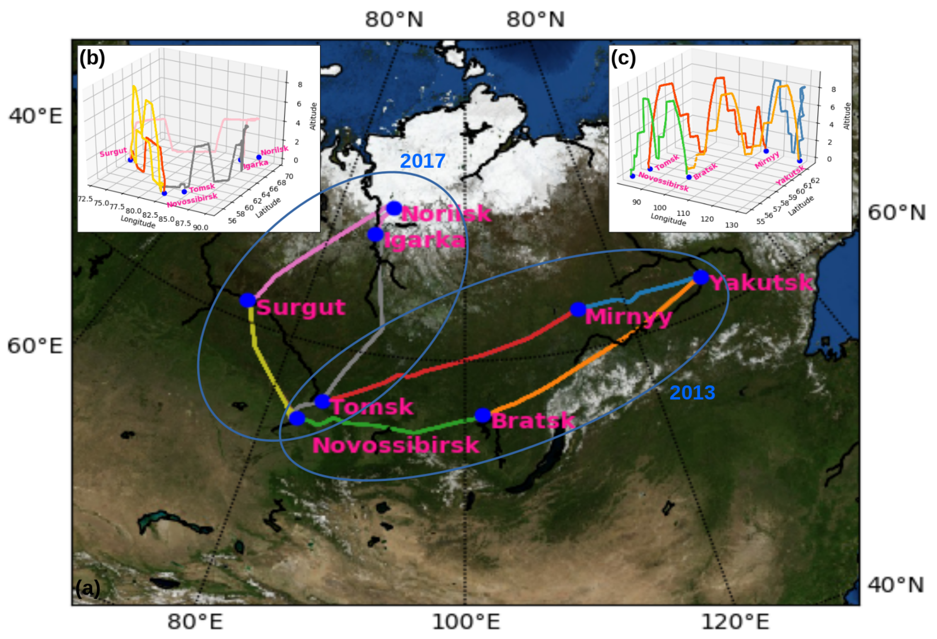
2.1. Campaign Description

Research aircraft operated by the Tomsk, Institute of Atmospheric Optics (IAO) has been flying along the transcontinental routes over central and eastern Siberia since 2006. Two airborne campaigns took place in July 2013 and June 2017 with a backscatter lidar and in-situ aerosol instruments installed on board the aircraft. The four flight tracks for each campaign are shown in Figure 1.

The flights were performed over (i) the major large Siberian cities (Novosibirsk, Tomsk, Krasnoyarsk, Yakutsk) (ii) the gas flaring fields of the Ob valley and the industrial city of Norilsk (iii) as well as over the Siberian taiga in order to track the long-range transport of emissions from wildfires and mid-latitude Eastern Asia. So the major aerosol sources could be included in this analysis. During these two airborne campaigns, downward looking backscatter lidar measurements were carried out but also in-situ measurements of trace gas concentrations and aerosol particle properties (size distribution, scattering properties). The aircraft performed various legs at low altitude (≈0.6 km) and between 4 and 8 km in order to sample different atmospheric layers. Only lidar data collected during flights above 4 km are used for the aerosol layer characterization.

2.2. Airborne Lidar System

The lidar system installed on board the Tu-134 aircraft is based on the aerosol lidar developed at IAO [26,27]. The lidar is included in the scientific equipment of the “Atmosfera” Common Use Center of IAO SB RAS. The transmitter module is based on a solid state Nd-YAG laser emitting 8 ns laser pulses at 1064 and 532 nm. The maximum output energy at 532 nm is 100 mJ with a repetition rate of 10 Hz and a beam divergence of 2.5 mrad. The optical receiver is a 150 mm diameter reception lens coupled with a 1 nm filter and two reception channels (co- and cross-polarization). The full geometrical overlap is obtained between 80 m and 150 m. In practice the first 200 m are not used to reduce the errors when estimating the overlap function correction in clear air region below the aircraft. The detection unit is composed of a photomultiplier coupled to an analog-to-digital converter (ADC) electronic system with a sampling rate range of 25–100 MHZ (i.e., a 1.5–6 m vertical resolution) and a resolution of 12 bits. The cross-polarization calibration is not sensitive enough to characterize the aerosol type and is mainly used to discriminate cloud and aerosol layers. The near infrared channel was not available during the aircraft campaigns. Attenuated backscatter signal in decimal logarithm >−2.3 with a signal above detection threshold in the depolarization channel is considered as cloud. The initial lidar data temporal averaging is 8 s and 1 min, respectively, for the 2013 and 2017 campaign. After cloud screening, data are averaged over 1–5 min to get a measurement range higher than 6 km.

2.3. In-Situ Measurements

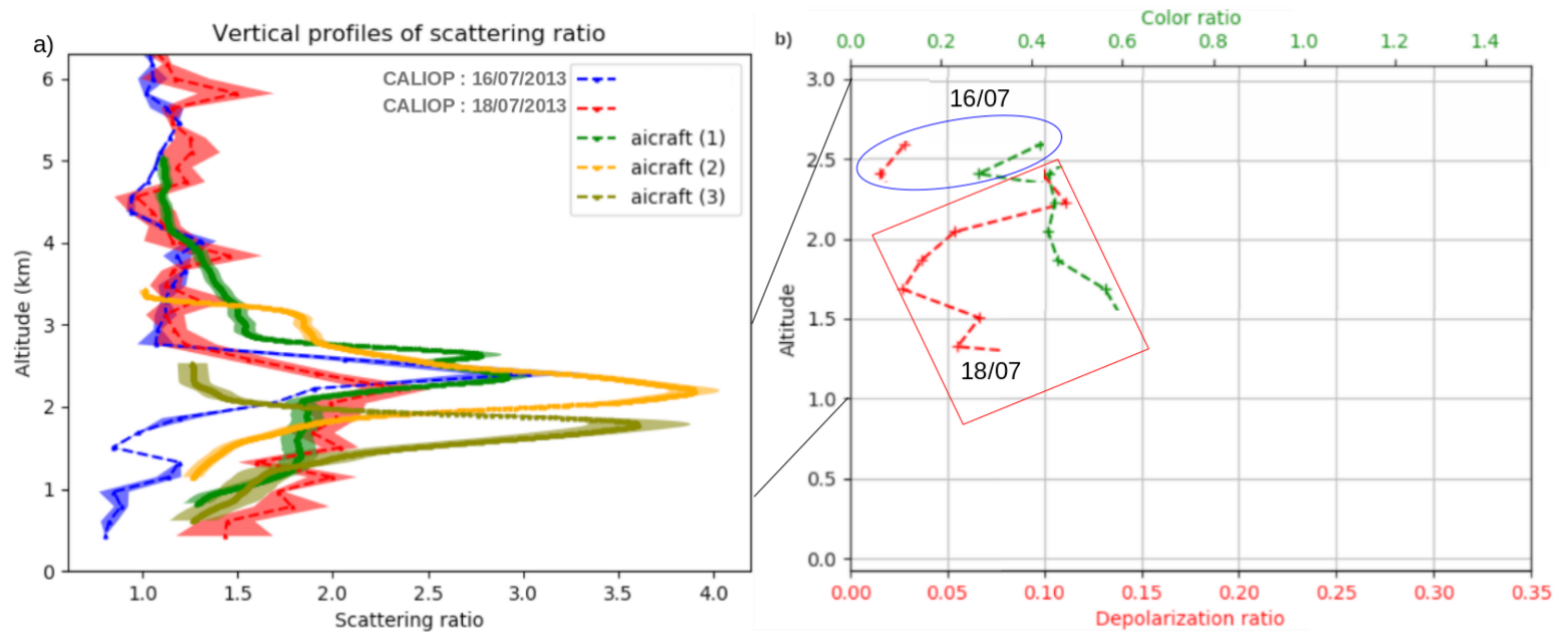
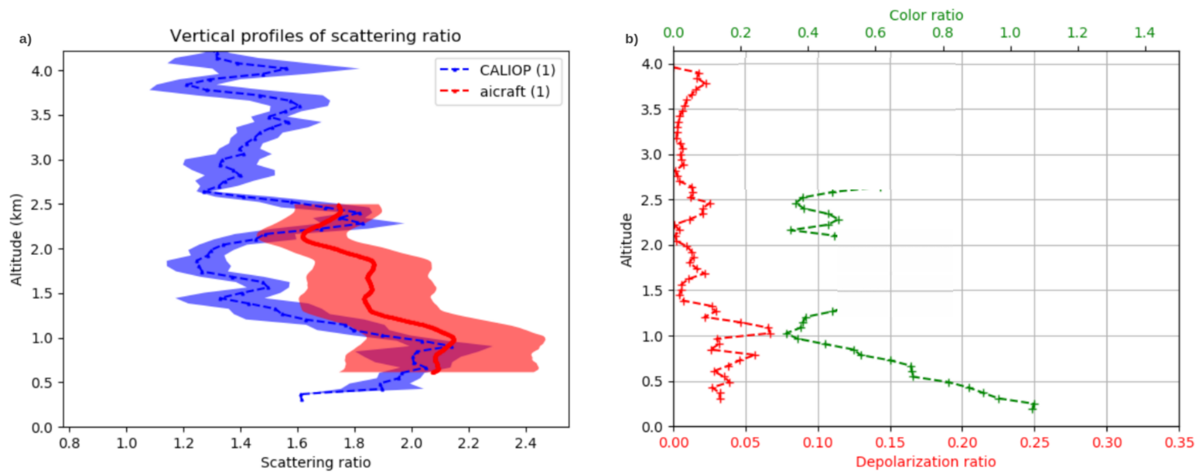
In-situ measurements include trace gas and aerosol measurements. CO measurement is performed using a fully automated CO analyzer based on a commercial infrared absorption correlation gas analyzer (Model 48C, TEI Thermo Environment Instruments, Franklin, MA 02038, USA). The instrument is described in [28]. The accuracy is 5 ppb (5% CO) for a 30 s integration time (i.e., the response time of the instrument) and the detection limit is 10 ppb.

CO₂, CH₄ and H₂O measurements were performed by means of the Picarro G2301-m gas concentration analyzer with a 5 s precision of 70 ppb for CO₂ and 0.5 ppb for CH₄. Water correction software automatically reports dry gas mole fractions.

Equivalent black carbon (EBC) mass concentration are measured using an aethalometer based on light attenuation by particles after collection on a filter [29]. The wavelength range between 0.4 and 1.1 $\mathsf{\mu }\mathrm{m}$ with a maximum near 0.9 $\mathsf{\mu }\mathrm{m}$. This instrument is sensitive to submicron particles. BC mass concentration (${\rho }_{BC}$) in $\mathsf{\mu }\mathrm{g}.{\mathrm{m}}^{-3}$ is converted from light absorption measurement ($ln\frac{I}{I_0}$) with the following relationship: ${\rho }_{BC}=697·C_f·ln\frac{I}{I_0}$, where $C_f$ is the correction factor between 0.5 and 1 taking into account the blackening of the filter. The EBC sensitivity is ≃ 0.01 $\mathsf{\mu }\mathrm{g}.{\mathrm{m}}^{-3}$.

The particle size distribution is fully characterized using two different instruments. Ultra fine particles concentration in the diameter range from 3 to 200 nm are measured using a diffusional particle sizer (DPS) consisted of an 8-channel automated diffusion battery (synthetic screen ADB; designed by ICKC SB RAS, Novosibirsk; Ankilow et al. [30], Ankilov et al. [31], Ankilov et al. [32]) coupled with a condensation particle counter (TSI CPC 3781). One scanning period of the DPS takes 80 s to derive size distribution in 20 size bins. Transmission efficiency for the airborne instrument is corrected for and is ≈0.997 in the 70–200 nm range and between 0.82 at 400 hPa and 0.89 at 1000 hPa for the 3–70 nm size range. All concentrations are reported at standard pressure and temperature (STP) conditions. Particle concentrations in 31 size bins in the range from 0.25 to 32 $\mathsf{\mu }$m are measured using a GRIMM 1.109 optical particle counter (GRIMM Aerosol Technik GmbH & Co. KG, Ainring 83404, Germany).

Meteorological parameters such as temperature, humidity and wind vector are measured routinely on-board using HYCAL sensor model IH-3602-C of Honeywell Inc. Temperature and relative humidity accuracies are 0.5 °C and 7%, respectively.

2.4. CALIOP Dataset

The CALIOP data analysis in this paper uses the vertical profiles of Level 1 (L1) Version 4.1 (V4.1) total attenuated backscatter coefficient (TAB) at 333 m horizontal resolution for both the visible (532 nm) and IR (1064 nm) channels and the TAB uncertainties are calculated using the ancillary parameters also available in the V4.1 L1 data products, namely the noise scale factor, laser energy, RMS random noise, calibration coefficient and amplifier gain. Cloud layer position and attenuation, aerosol type and lidar ratio are available at 5 km horizontal resolution in the V4.2 L2 layer cloud and aerosol data products. All the CALIOP cloudy profiles are removed regardless of the cloud aerosol discrimination (CAD) score to ensure that no clouds are accounted for in the analysis of TAB. In this work the CALIOP TAB and lidar ratio are horizontally averaged in the FLEXPART footprint corresponding to the aircraft observation (generally of the order of 100 km). The Fernald forward inversion needed to calculate the AOD and the backscatter ratio vertical profile at 532 nm (ratio of the total backscatter including molecular and aerosol component over the molecular backscatter) is made from the top altitude of the highest aerosol layer [33]. The uncertainty of the lidar ratio have been taken from [24] when calculating the error on the retrieved total backscatter coefficient. The particle linear depolarization ratio at 532 nm is calculated using the ratio of the perpendicular and parallel component of TAB and the backscatter ratio. The particle color ratio is defined as the ratio of the aerosol backscatter coefficient at 1064 and 532 nm. Both the particle linear depolarization ratio and the particle color ratio are not calculated for backscatter ratio at 532 nm less than 1.5 to remove noisy values.

3. Methodology of the Aircraft Data Analysis

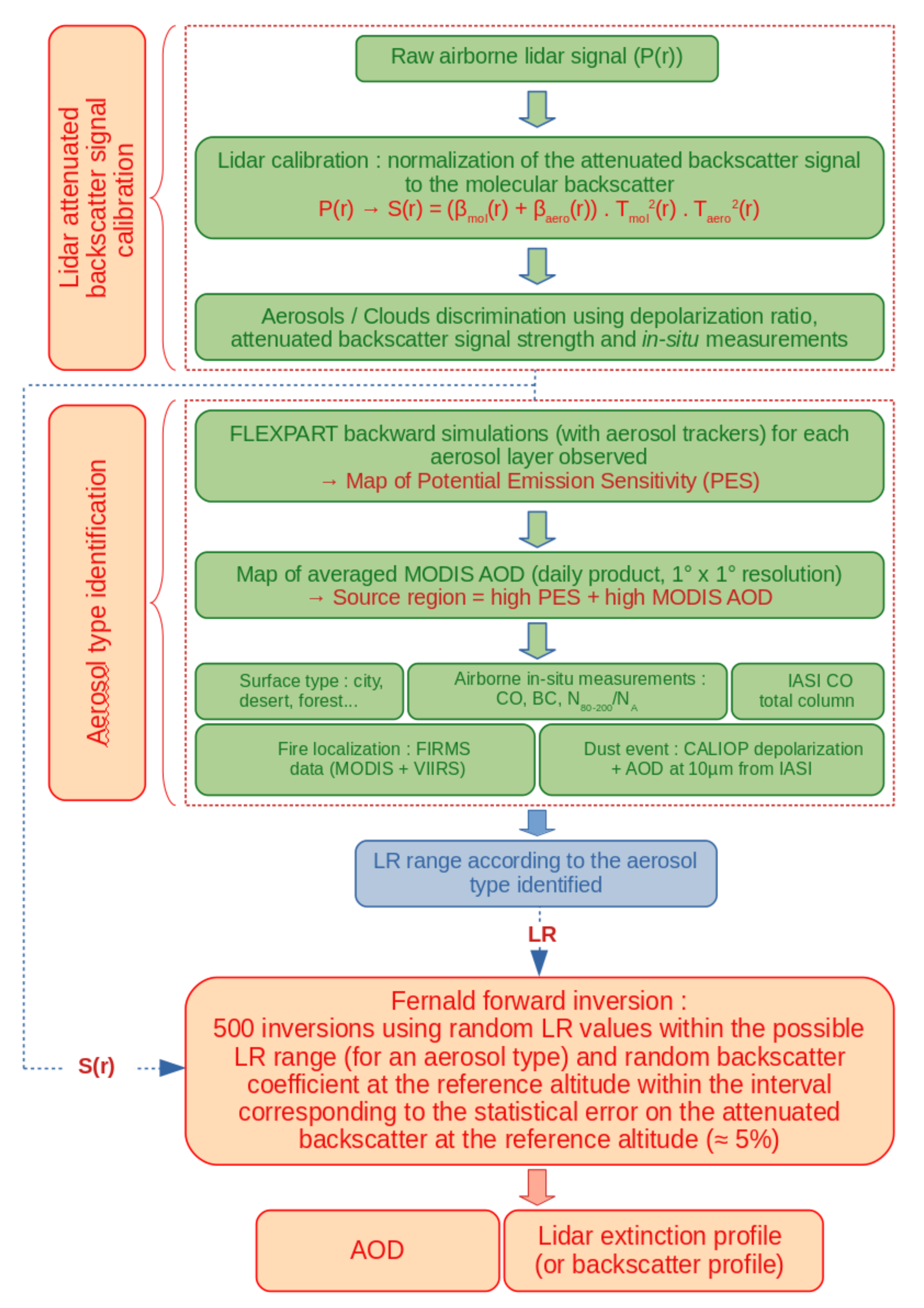
3.1. Aircraft Data Processing

The lidar calibration is performed several times during each flight using a normalization of the attenuated backscatter signal (PR2) to molecular backscatter in the range 200–700 m below the aircraft with a 1–5 min temporal resolution. Flight sections without aerosol/cloud occurrence are determined using the in-situ aircraft measurements (total aerosol concentrations from the Grimm instrument <15 particles.cm${}^{-3}$). The vertical profile of molecular backscatter was estimated from the 0.75${}^{°}$ ERA-Interim ECMWF meteorological analysis [34]. To account for the the overlap function between the field of view of the laser and the telescope, the mean altitude dependency of the ratio between PR2 and the molecular backscatter is determined for each flight in the 0–700 m altitude range below the aircraft using only profiles with no cloud and aerosol layers. The calibration accuracy is then of the order of 5–10% due to the mean signal statistical uncertainty (<3%) and the assumption on the reference backscatter ratio being unity in the calibration range (≈5%).

The aerosol optical depth and the backscatter ratio vertical profile retrieval are based on the Fernald forward inversion of the calibrated PR2 [33], assuming a range independent value of aerosol lidar ratio (LR). The LR value is chosen according to the aerosol type identified following the methodology described in Section 3.2. This is somewhat similar to the approach proposed by [23] for the analysis of the CALIPSO aerosol extinction profiles. The range of the LR is taken from several papers providing measured LR either with a HSRL lidar or a Raman lidar for a large range of aerosol types. This will be discussed for each case study described in this paper.

To estimate the uncertainty of the retrieved backscatter ratio, 500 inversions were performed using random LR values within the possible LR associated to an aerosol type and random backscatter coefficient at the reference altitude within the interval corresponding to the statistical error on the attenuated backscatter at the reference altitude (≈5%). The complete methodology for the lidar data analysis is summarized in the upper panel of Figure 2.

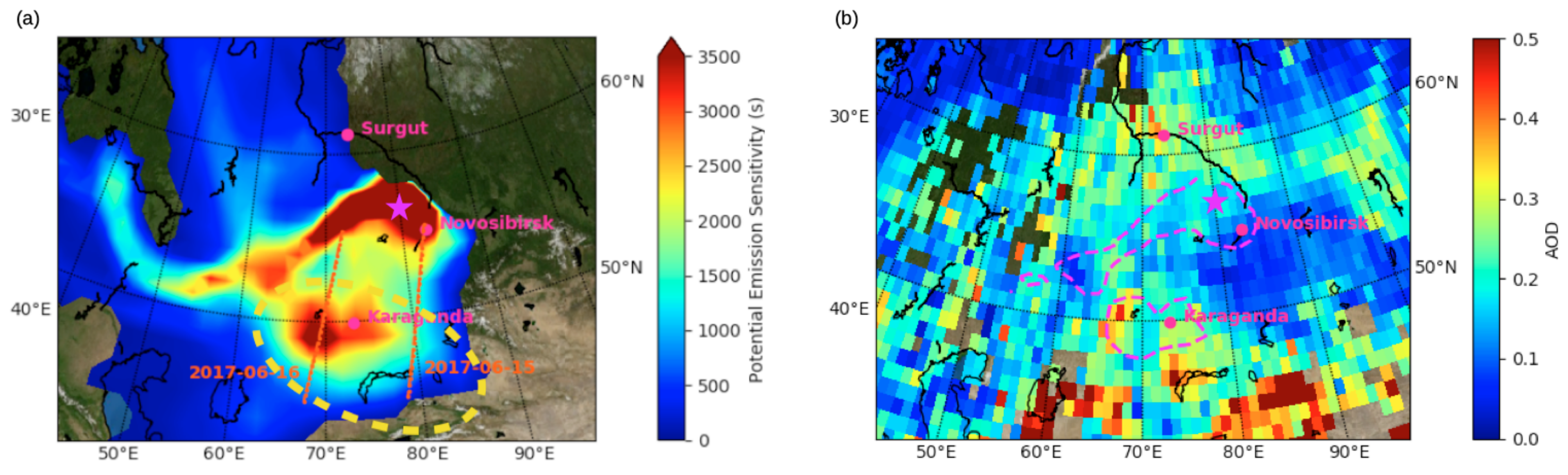
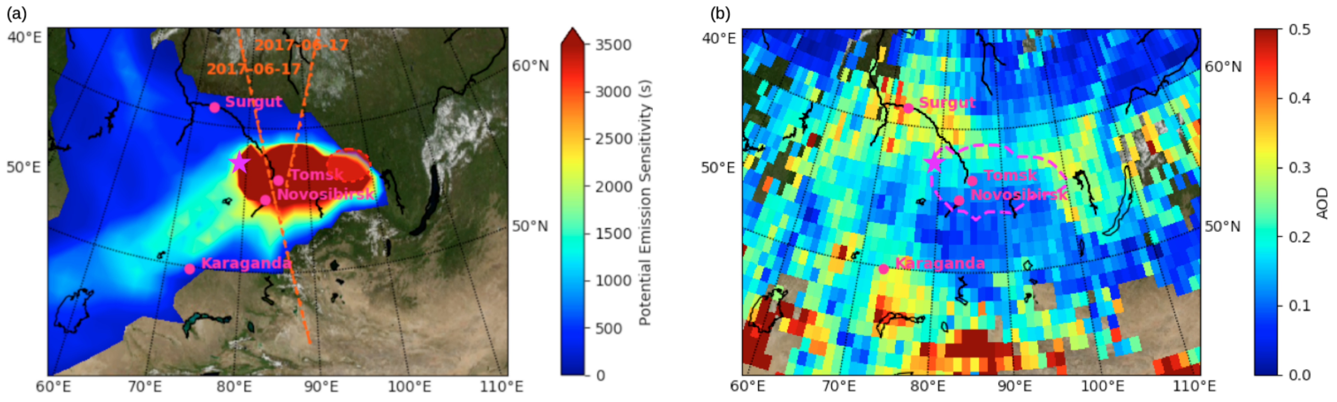
3.2. Identification of the Aerosol Sources

Aerosol types of the layers observed by the airborne lidar were characterized using first the Lagrangian FLEXible PARTicle dispersion model (FLEXPART). FLEXPART is a Lagrangian model designed for computing the long-range transport, diffusion, dry and wet deposition, of air pollutants or aerosol particles backward or forward from point sources using a large number of particles [35,36]. For our study particle dispersion calculations are performed by including aerosol tracer removal processes by dry and wet deposition in the cloud and under the cloud. For each aerosol layer identified in a lidar profile, 5–10 days backward simulations of the spatial distribution of 10,000 particles released in a 1 km thick altitude zone is made. The occurrence of clouds is calculated by FLEXPART using the relative humidity fields. The meteorological fields used for the simulations (including precipitation rates) are operational ECMWF field at T255 horizontal resolution (≈80 km) and with 153 model vertical levels. FLEXPART simulations provide maps of Potential Emission Sensitivity (PES) for each aerosol layer observed by the airborne lidar. These maps represent the areas that have most influenced the observations including the correction due to the losses of the tracer [37]. The PES maps are always compared to the AOD${}_{550}$ maps at 550 nm from the Level-3 MODIS Atmosphere Daily Global Gridded Product (1${}^{°}$ × 1${}^{°}$ resolution) in order to identify the effective aerosol source regions. Only data with high quality flag have been considered in this work.

The sources of biomass-burning aerosol are identified using the daily fire radiative power (FRP) maps based on NASA Fire Information for Resource Management System (FIRMS) from MODIS observations [38] and the Visible Infrared Imaging Radiometer Suite (VIIRS) [39]. Significant biomass burning aerosol production is taken into account only if the daily FRP is higher than 0.3 GW and the fire lifetime higher than three days and if the CO tropospheric column measured by IASI (Infrared Atmospheric Sounding Interferometer) is higher than the monthly background CO column [40,41,42] (Data set Clerbaux [43]). No quality flag is used, but cloudy pixel have been removed.

Dust outbreaks from the Eastern Asia desert are only taken into account if the aerosol optical depth measured by IASI at 10 $\mathsf{\mu }$m (AOD_{10$\mathsf{\mu }$m}) is greater than 0.08 in the area with elevated PES [44,45,46] and when CALIOP aerosol depolarization ratio is greater than 15% in the same area [16,47,48]. No quality flag is applied to this data set.

The location of flaring sources is based on the anthropogenic emissions ECLIPSEv4 data-set (Evaluating the Climate and Air Quality Impacts of Short-Lived pollutants) described in [49]. This inventory includes in particular the gridded methane emissions from gas flaring in the Russian Arctic at a 0.5${}^{°}$ × 0.5${}^{°}$ horizontal resolution. A threshold of 50 moles.km${}^{-2}$/h has been applied to the methane emissions to select areas that could potentially be defined as flaring sources. Urban pollution aerosol sources are considered only when large cities (>500,000 inhabitants) are included in the area with high PES (≥2500 s). The elevated CO tropospheric column (>2.10${}^{18}$ $\mathrm{molecule}.{\mathrm{cm}}^{-2}$) in the same area is also mandatory to select cities with significant industrial and urban combustion sources [50].

In addition to this first guess for the aerosol type identification based on the FLEXPART simulation analysis, in-situ aircraft measurements of CO concentration, black carbon (BC) mass concentration and aerosol size distribution are also analyzed for aircraft ascent or descent across the aerosol layer observed by the airborne lidar. Excess of CO ($\mathsf{\Delta }$CO), i.e., the difference with the background CO concentration taken as the minimum of CO measured during the two campaigns in the lower troposphere (0–5 km), must reach 30 ppb for biomass burning aerosol and gas flaring emission (Paris et al. [4]). Black carbon mass concentrations is also used to identify combustion aerosol: BC > 0.5 $\mathsf{\mu }\mathrm{g}.{\mathrm{m}}^{-3}$and BC maximum correlated with elevated $\mathsf{\Delta }$CO. The ratio of the aerosol concentration in the cloud condensation nuclei size range between 80 and 200 nm (N${}_{80-200}$) over the aerosol concentration in the Aitken mode (N${}_A$) between 15 and 80 nm is used to identify the aerosol aging [51,52,53]. The complete methodology for the aerosol type identification is summarized in the lower panel of Figure 2.

4. Aircraft Campaign Data Analysis

Six flights have been selected during the 2013 and 2017 campaigns, because they correspond to different aerosol sources. The lidar vertical cross-section of the calibrated attenuated backscatter (PR2) have been used to identify the horizontal and vertical extent of the aerosol layers (532 nm backscatter ratio larger than 1.5). For each aerosol plume, the aerosol type is retrieved using the methodology described in Section 3.2 and the AOD${}_{532}$ of the layer is calculated with a constant LR in the layer as explained in Section 3.1.

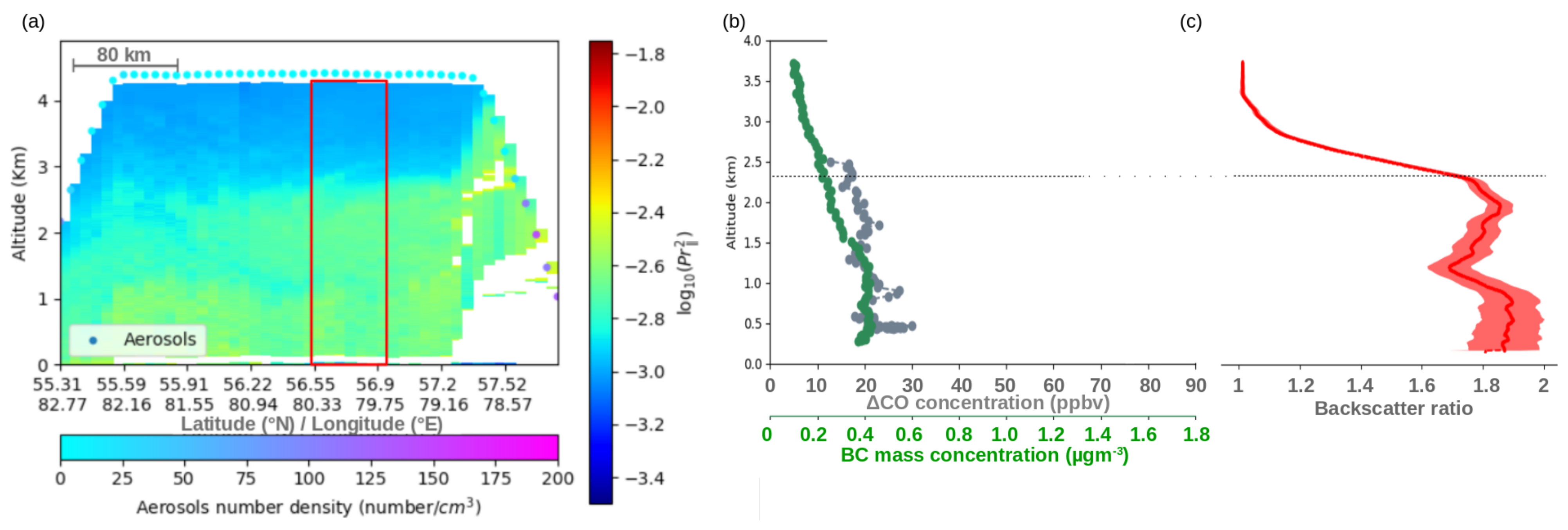
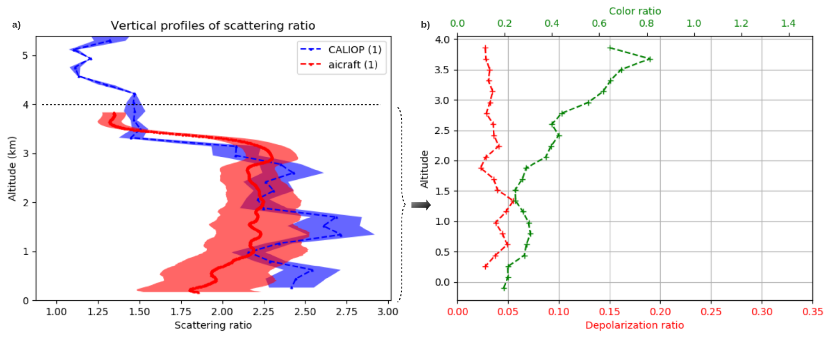
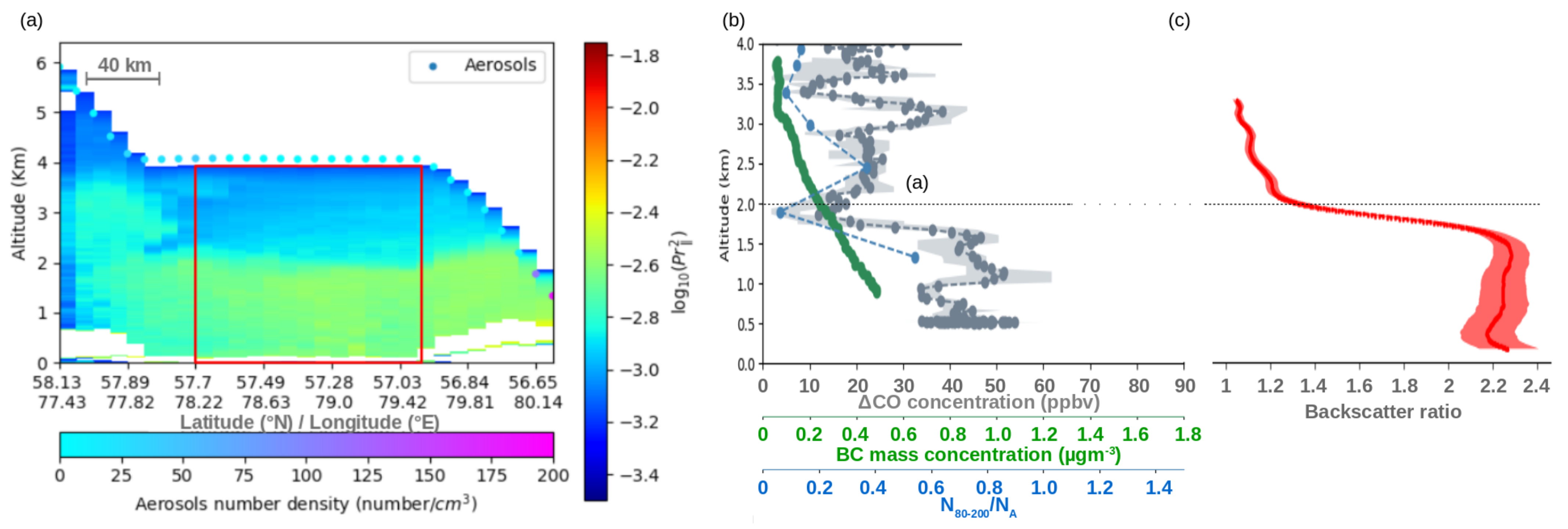
4.1. Dusty Aerosol Mixture

On 16 June 2017 at 5 UT the aircraft flew between Novosibirsk and Surgut above the Ob Valley. The PR2 latitudinal cross-section when the aircraft is flying at 4.2 km, shows an aerosol layer in the 0 and 2.5 km altitude range with a 150 km horizontal extent (Figure 3). Clouds (high backscatter and high depolarization ratio) are encountered at 57.5 N when descending to a lower flight level near 500 m.

Two areas with PES ≥ 2500 s for the aerosol layer in the altitude range 0 to 2.5 km correspond to two regions with elevated 4-day averaging of the MODIS AOD${}_{550}$ (>0.2): the region 1 is the industrial area (55${}^{°}$ N, 80${}^{°}$ E) located North East of Novosibirsk and the region 2 from 65${}^{°}$ E to 75${}^{°}$ E is above Kazakhstan at 50${}^{°}$ N (Figure 4). Fires are detected by MODIS and VIIRS during 3 days (FRP < 0.2 GW) in the region 2 over Kazakhstan, while the tropospheric CO column measured by IASI is higher than 2.0 × 10${}^{18}$ $\mathrm{molecule}.{\mathrm{cm}}^{-2}$ in the same area (Figure 5a). The tropospheric CO column is also elevated (1.5–1.8 × 10${}^{18}$ $\mathrm{molecule}.{\mathrm{cm}}^{-2}$) at 58${}^{°}$ N, 80${}^{°}$ E in the region 1 (Figure 5a).

The role of dust emission is also significant for this case study when looking at the 4-day average of the AOD_{10$\mathsf{\mu }$m} measured by IASI which is in the range 0.15–0.35 in region 2 above Kazakhstan (Figure 5a). A CALIOP overpass on 16 June 2017 at 21 UT also shows high particle linear depolarization ratio (15–20%) and a particle color ratio (ratio of aerosol backscatter coefficient at 1064 and 532 nm) in the range 0.3–0.7 in the lower troposphere at 50${}^{°}$ N, 70${}^{°}$ E in region 2 (Figure 5b). An aerosol depolarization ratio less than 20% is consistent with polluted dust aerosol (Tesche et al. [47], Gro et al. [48], Burton et al. [15], Gro et al. [16]). In the flight area, IASI also detected a AOD_{10$\mathsf{\mu }$m} between 0.08–0.1, i.e., smaller than above Kazakhstan, but being just above the dust detection threshold of 0.08. The aerosol layer observed by the airborne lidar at 57${}^{°}$ N, 80${}^{°}$ E can be therefore considered as a mixture of dust, industrial pollution the Ob Valley and aged smoke.

When looking at the in-situ measurements made by the aircraft during the descent at 57.5${}^{°}$ N, $\mathsf{\Delta }$CO range is between 20 and 30 ppbv up to 2.5 km and the BC mass concentration increases from 0.2 $\mathsf{\mu }$g.m${}^{-3}$ at 2 km to 0.4 $\mathsf{\mu }$g.m${}^{-3}$ at 500 m (Figure 3b). These moderate values of $\mathsf{\Delta }$CO and BC compared to other flights (

Table 1. Aerosol layer altitude, age and optical properties (AOD, color ratio, depolarization ratio) together with BC, $\mathsf{\Delta }$CO concentration and N${}_{80-200}$/N${}_A$ for the six aerosol layers selected in this work.

Aerosol Type	Dust/Smoke	Smoke from	Smoke from	Gas Flaring	Urban	Urban
	Emissions from	Siberian Fires	Siberian Fires	Emissions	Emissions of	Emissions from
	Kazakhstan				Siberian Cities	Northern China
Layer Altitude	1.0 (2.0)	2.2 (3.5)	0.9 (1.8)	1.5 (3.2)	1.5 (3)	3.0 (4.5)
mean (maximum), km
Layer age	Aged	Fresh	Aged	Fresh	Fresh	Aged
$\mathsf{\Delta }$CO, ppbv	20	35–45	45–55	30–40	50	60–80
BC concentration	0.2–0.4	1.5	0.4–0.5	0.4–0.5	0.2	0.2
in $\mathsf{\mu }$g.m${}^{-3}$
N${}_{80-200}$/N${}_A$	-	0.15	0.6	0.3–0.6	0.5	0.8–1.0
Aircraft AOD${}_{532}$	0.1 ± 0.03	0.12 ± 0.02	0.16 ± 0.03	0.21 ± 0.06	0.15 ± 0.09	0.19 ± 0.01
CALIOP AOD${}_{532}$	0.11 ± 0.04	0.11 ± 0.04	0.17 ± 0.07	0.32 ± 0.09	0.18 ± 0.06	0.21 ± 0.07
MODIS AOD${}_{550}$	0.11 ± 0.02 *	0.19 ± 0.02 *	0.22 ± 0.04 **	0.33 ± 0.05 **	0.29 ± 0.05 *	-
CALIOP Depolarization	4–5	3–10	5–12	3–5	1–5	1–5
ratio, %
CALIOP color ratio	0.5–0.7	0.4	0.7	0.2–0.4	0.3–0.5	0.6

Time slot for the selection of MODIS observations near the aircraft: * ±1 h, ** ±6 h.

) are also consistent with a dusty aerosol mixture.

The AOD${}_{532}$ and the backscatter ratio are calculated from the airborne lidar data for a 6 min average profile shown by the red rectangle in Figure 3. The lidar ratio range is between 29 and 49 sr according to [14,15] for a dusty mix aerosol type when using HSRL lidar measurements. Similar values (38 ± 7 sr) are reported by [54] with a Raman lidar in China for a dust plume mixed with urban emissions. The corresponding airborne lidar AOD${}_{532}$ is then 0.1 ± 0.03 (Table 1). The average AOD${}_{550}$ measured by MODIS within ±1 h and ±100 km around the lidar observations is similar (0.11) and shows very small variations (0.02). Looking at the FLEXPART PES analysis a CALIOP granule on 15 June 2017, 21UT also crosses the same air masses with the dusty aerosol mixture. The 80 km horizontal average of the backscatter ratio vertical profile at 44${}^{°}$ N is calculated using a Fernald inversion and the CALIOP lidar ratio available in the CALIOP Version 4.2 aerosol data products. It shows an aerosol layer up to 2.5 km but the backscatter ratio is smaller than the aircraft data between 1.5 and 2.5 km and shows a sharp peak up to 2.4 at 1 km (Figure 6a). The CALIOP particle color ratio ≥ 0.5 (Figure 6b) is in agreement with a significant fraction of coarse size aerosol [55]. The CALIOP aerosol layer classification is indeed 77% polluted dust, 6% dust, 6% clean continental and 11% elevated smoke, with an average lidar ratio of 55.8 sr and a low average AOD${}_{532}$ of the order of 0.11 ± 0.04.

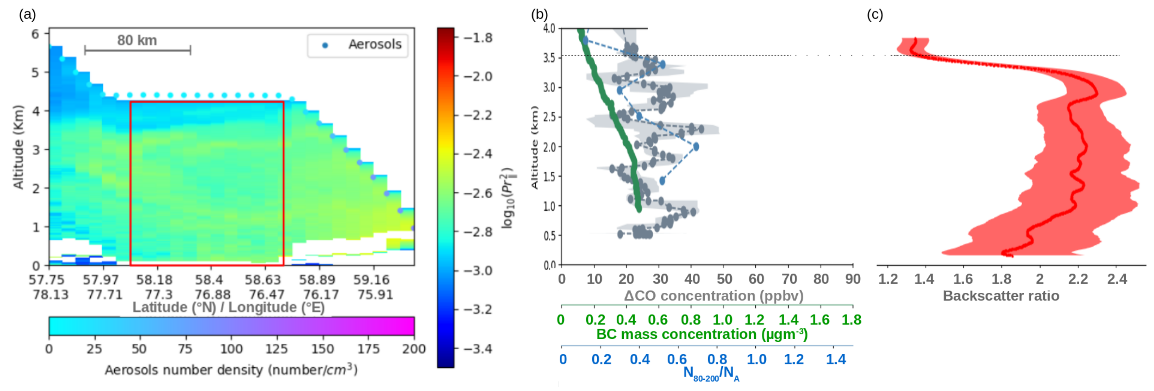
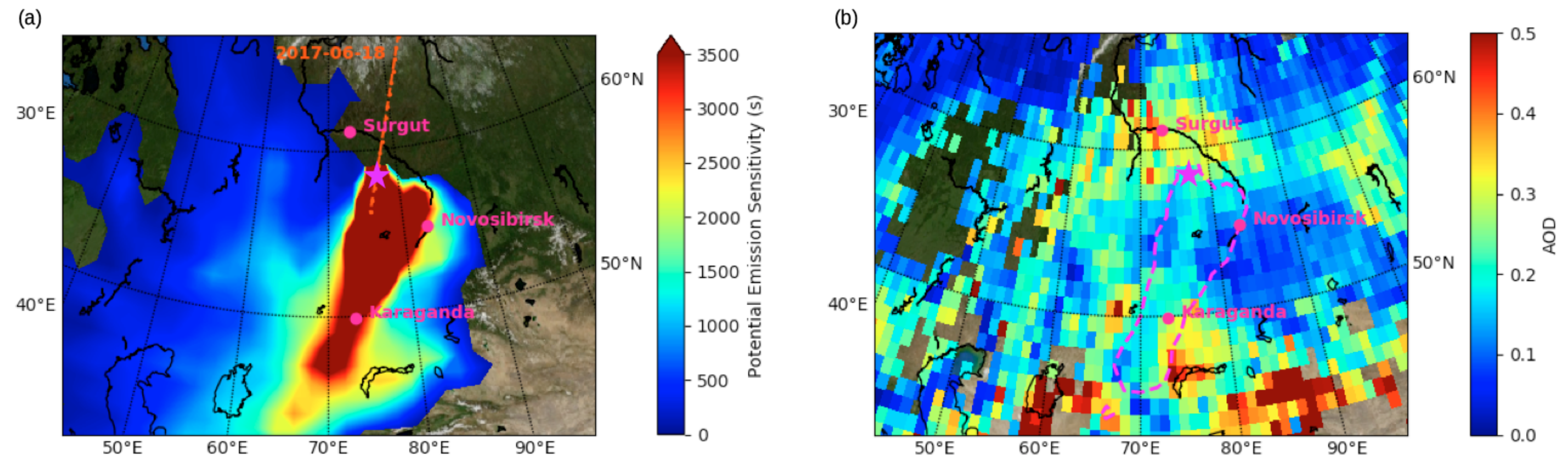
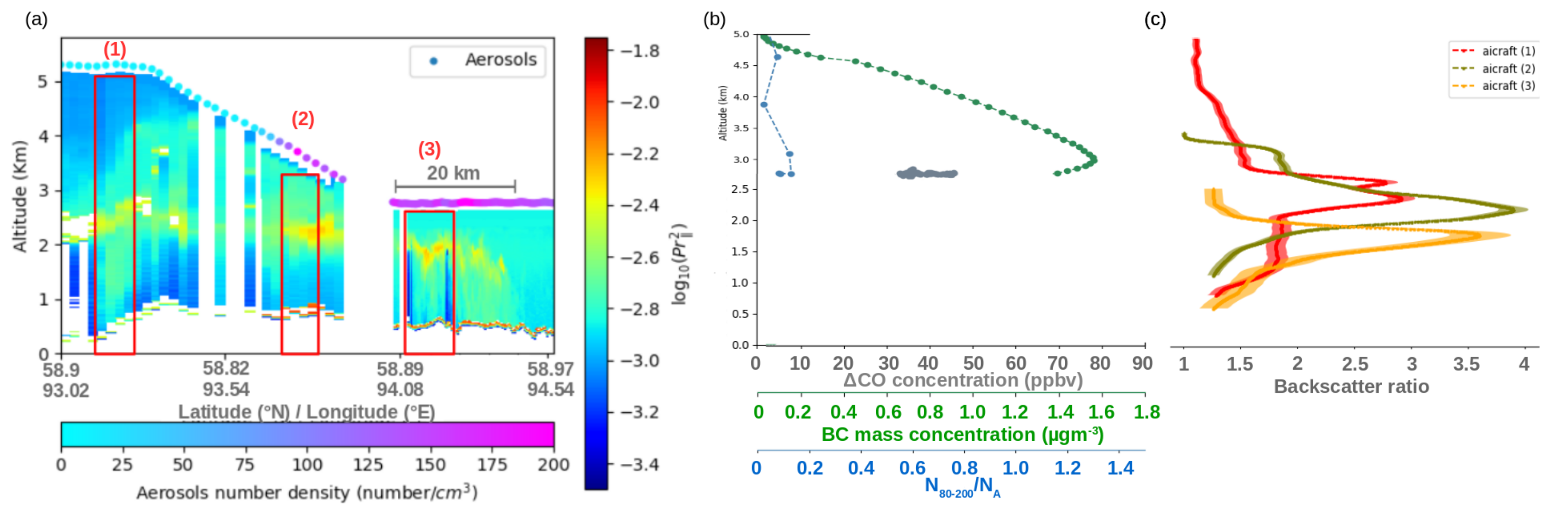
4.2. Ob Valley Gas Flaring Emissions

On 18 June 2017, aerosol layers in the 0–3.5 km altitude range have been observed at higher latitudes during a second flight between Novosibirsk and Surgut above gas and oil extraction fields in the latitude range 58${}^{°}$–59${}^{°}$ N. The layer is still very well identified as the aircraft approaches Surgut and in-situ measurements during the descent to Surgut have been made in the same aerosol layer (Figure 7).

Potential emission sensitivity higher than 2500 s and coupled with daily MODIS AOD${}_{550}$ higher than 0.2 (Figure 8) shows that this aerosol layer corresponds to a mixture of an air mass from the Ob Valley (55${}^{°}$ N–60${}^{°}$ N, 75${}^{°}$ E) with air masses still transported from Kazakhstan, but with little influence from the fire region at 67${}^{°}$ E. The IASI CO tropospheric column maximum of 2.0 × 10${}^{18}$ molecule.cm${}^{-2}$ for the 15–18 June 2017 average which is above the Ob Valley at 59${}^{°}$ N, 75${}^{°}$ E, is now very close to the aircraft position (Figure 9). Contrary to the previous case, the 4-day average of the AOD_{10$\mathsf{\mu }$m} (0.06) in the aircraft flight area is also below the dust detection threshold of 0.8, even though sensitivity to dust emission from Kazakhstan is still highlighted by the PES analysis (Figure 9). During the descent to Surgut at 59${}^{°}$ N, aircraft in-situ measurements (Figure 7b) also show $\mathsf{\Delta }$CO concentrations up 40 ppbv and BC mass concentration of 0.5 $\mathsf{\mu }\mathrm{g}.{\mathrm{m}}^{-3}$ in the 1–2 km altitude range which indicate that local pollution sources have been transported up to 2 km on 18 June 2017. The moderate value of the ratio N${}_{80-200}$/N${}_A$ (0.3–0.6) is also consistent with a significant fraction of fresh emissions from the Ob valley area. A nighttime CALIOP overpass is available in the same area at 75${}^{°}$ E and on the same day (19 h later), showing a backscatter ratio vertical profile with a shape and magnitude similar to the aircraft lidar observations (Figure 10a). The very weak aerosol depolarization ratio (<5%) and color ratio (0.2–0.5) measured by CALIOP in the latitude band 57${}^{°}$–58${}^{°}$ N correspond to aerosol optical properties typical of continental pollution (Figure 10b). We can conclude then that the aerosol layer sampled by the airborne lidar at 58${}^{°}$–59${}^{°}$ N on 18 June below 3.5 km is mainly related to the Ob Valley aerosol emissions and is not significantly influenced by the Kazakhstan dust and biomass burning emissions.

Few specific studies of aerosol plumes from flaring zones with a Raman or HSRL lidar system have been published for flaring emissions. Chazette et al. [56] reported LR of the order of 71 sr at 355 nm at Hammerfest (70.6${}^{°}$ N, 23.6${}^{°}$ N), Northern Norway, for a mixture of flaring emissions from a single industrial source and aerosol transported from the Murmansk region (68${}^{°}$ N, 33${}^{°}$ E) in Russia. However, this case is hardly comparable to the case of the Ob valley, which has many flaring sources. The LR range of 40–50 sr, measured in Tomsk by [11] above the boundary layer between 2.5 and 5 km altitude using measurements with a Raman lidar at 532 nm in April and May 2007, is probably a better indicator of the range of LR for the flaring emissions of the Ob valley. The April–May 2007 period was not impacted by fires in Siberia and long distance transport was mainly controlled at 500 hPa by a westerly or northerly flow from the Ob valley region (22 days out of 31). The lidar ratio range is then chosen between 40 and 50 sr in order to calculate the AOD${}_{532}$ and the backscatter ratio from the airborne lidar data for a 6 min average profile shown by the red rectangle in Figure 7a. The corresponding AOD${}_{532}$ for the airborne lidar is then 0.21 ± 0.06 (Table 1), two times larger than the previous dusty mix case observed at 57${}^{°}$ N two days earlier. The average AOD${}_{550}$ measured by MODIS within ±6 h and ±100 km around the lidar observations is also larger (0.33 ± 0.048). For a time slot of ±24 h around the aircraft measurement time, MODIS AOD${}_{550}$ distribution is of the order of 0.23 ± 0.07. Regarding the CALIOP observations shown in Figure 10, 55% of the layers are classified as “Polluted Dust” and 45% as “Elevated Smoke” with a mean lidar ratio of 60 sr. The corresponding AOD${}_{532}$ (0.32 ± 0.09) is very close to the MODIS observation at the same wavelength (0.35 ± 0.05) assuming an Angström exponent of 2 for this polluted continental plume. Therefore, the upper boundary (50 sr) of the LR range assumed for gas flaring is more likely.

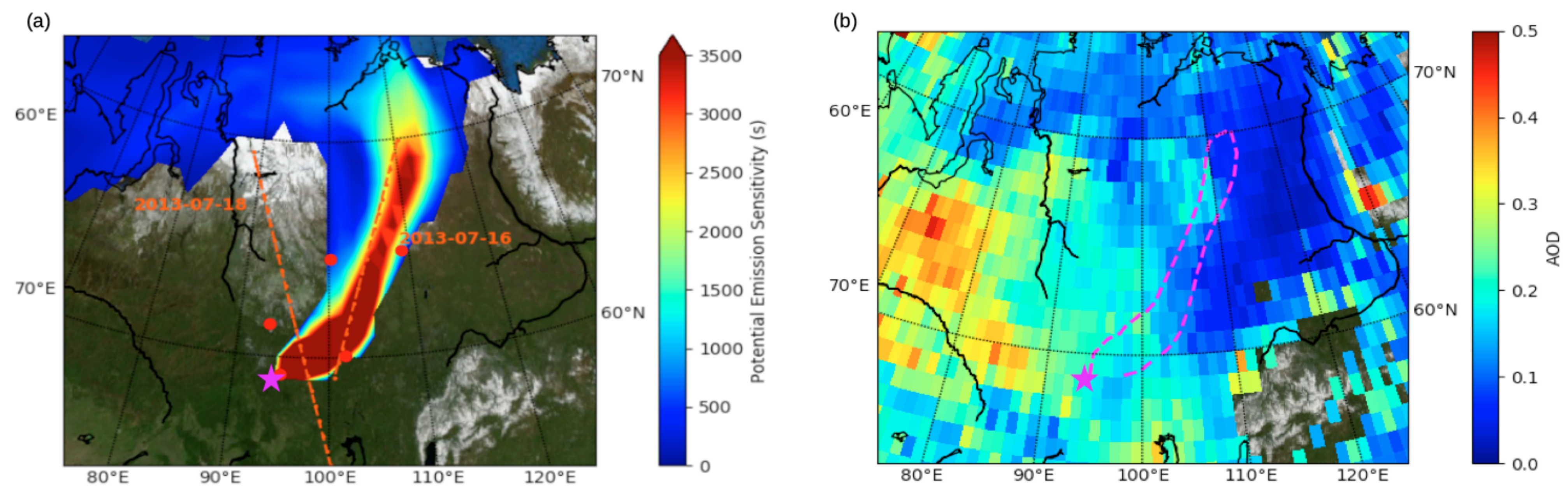
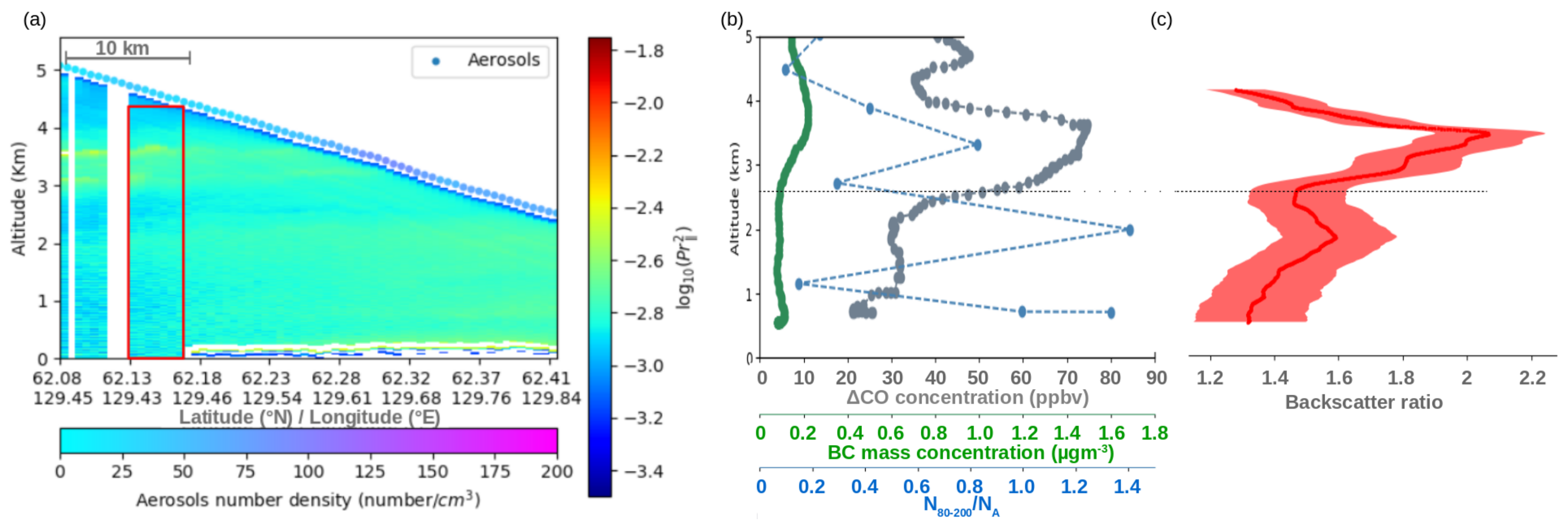
4.3. Fresh Forest Fire Plume

The aircraft flew on 19 July 2013 at 6 UT near a region with numerous forest fires above Northern Siberia between 60${}^{°}$ N and 65${}^{°}$ N, and 90${}^{°}$ E and 100${}^{°}$ E. The airborne lidar detected a 500-m thick aerosol layer in the altitude range 2–4 km with a backscatter ratio of the order of 3.5 (Figure 11) related to one of these fires. The aerosol plume sampled by the aircraft has a West–East cross section of 50 km. The PES map calculated by FLEXPART (Figure 12) shows no aerosol transport from large cities or pollution sources. Active forest fires with a lifetime around 3 days and FRP up to 0.2 GW took place at 66${}^{°}$ N, 108${}^{°}$ E from 17 to 19 June 2013 and an active fire was observed at the aircraft location (58${}^{°}$ N, 95${}^{°}$ E) on 19 June with a FRP of 0.18 GW and a lifetime of 1–2 days. A fresh forest fire plume is then responsible for the aerosol layer seen by the lidar with a backscatter ratio higher than 3.5. The aircraft in-situ measurements during the aircraft descent at 94${}^{°}$ E indeed show BC mass concentration up to 1.6 $\mathsf{\mu }$g.m${}^{-3}$ and $\mathsf{\Delta }$CO up 40 ppbv at 3 km, and the low N${}_{80-200}$/N${}_A$ ratio (0.1–0.15) is consistent with the sampling of a fresh fire plume.

To calculate the backscatter ratio and the extinction vertical profile, we assume a lidar ratio range of 33 sr to 46 sr based on the paper of [14] who provide LR for both fresh and aged biomass burning plumes in Northern America. This is also in good agreement with the 45 sr lidar ratio at 532 nm reported by [57] for a fresh fire plume in Southern Europe. The AOD${}_{532}$ and backscatter ratio are calculated for three 40 s average profile shown by the red rectangles at 93.2${}^{°}$ E, 93.7${}^{°}$ E and 94.1${}^{°}$ E in Figure 11. The backscatter ratio reaches 4 in a 1 km thick layer for two sections and 3 for the other one. The AOD${}_{532}$ are identical (0.118 ± 0.027) for layers (1) and (2) and less (0.085 ± 0.026) for the layer (3), knowing that the latter is underestimated by at least 35% since the layer may extend above 2.5 km when looking at the high concentrations measured by the aerosol counter at 2.8 km (200 particles/cm${}^3$). The MODIS AOD${}_{550}$ for ±1 h and ±100 km around the aircraft observations are significantly higher than the airborne lidar AOD${}_{532}$ (0.19 ± 0.02). Such large differences are not surprising for spatially well defined aerosol plume close to the emission sources. Indeed MODIS AOD${}_{550}$ becomes 0.155 ± 0.07 when the averaging time period is ±24 h. No CALIOP track was close enough to the aircraft to be compared with the same aerosol plume. However, a comparison was made with two CALIOP overpasses right above other fires with similar FRP (0.18 GW) located at 62${}^{°}$ N on 16 July 2013 at 19 UT and at 59${}^{°}$ N on 18 July 2013 at 05 UT (Figure 13). The fires detected by CALIOP also show the altitude of backscatter ratio maximum in the range 2–3 km but with smaller scattering magnitude (of the order of 2.5). The color ratio range is 0.3–0.4 at the altitude of the fire plume, while the depolarization ratio is quite variable but remains below 10% (Figure 13). The aerosol type identified by CALIOP are 58.5% and 100% polluted continental for, respectively the fires detected on 16 and 18 July 2013. No elevated smoke is detected because the layers remain below 3 km. The lidar ratio are taken as 59 and 70 sr for these two days, while the AOD${}_{532}$ retrieved by CALIOP become 0.09 ± 0.04 and 0.17 ± 0.08. The CALIOP AOD${}_{532}$ for fresh fires is in better agreement with the airborne lidar observations on 16 July 2013 probably because on this day CALIOP assumes a 59 sr lidar ratio more comparable to the range of LR for fresh fires.

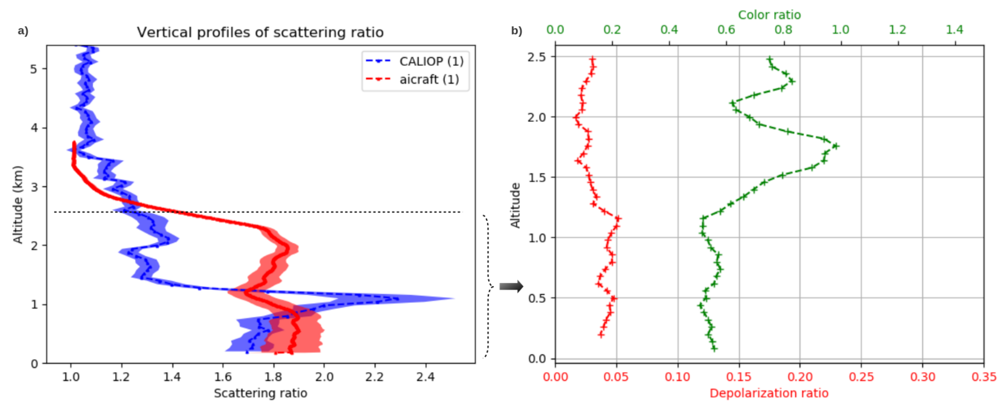
4.4. Aged Forest Fires

It is also interesting to investigate data corresponding to aged fires which should provide larger extinction according to previous studies [15,47,58]. Part of the 18 June 2017 flight descending to Novosibirsk at 3 UT meets this objective. The latitudinal cross-section PR2, when the aircraft flies at 4 km, shows a layer of aerosol in the altitude range of 0 and 2 km with an horizontal extension of 120 km (Figure 14).

The PES calculated by FLEXPART between 500 m and 2 km at 57.4${}^{°}$ N (Figure 15) shows that aerosol emissions are from an area between 80${}^{°}$ E and 100${}^{°}$ E at 57${}^{°}$ N, while the highest MODIS AOD${}_{550}$ in this area are related to forest fires which occurred 100${}^{°}$ E North of Irkutsk (0.05 < FRP < 0.2 GW). The CO tropospheric column measured by IASI North East of Irkutsk (Figure 16) is of the order of 2.5 × 10${}^{18}$ molecule.cm${}^{-2}$, while it remains in the range 1.5–2.0 × 10${}^{18}$ molecule.cm${}^{-2}$ above the cities of Tomsk, Novosibirsk and Krasnoyarsk also located in the area with high PES (≥2500 s). Forest fire plumes from Eastern Siberia at 2000 km from the aircraft can explain the aerosol layers seen by the airborne lidar at 57.49${}^{°}$ N, 78.63${}^{°}$ E on 18 June 2017. In-situ aircraft measurements (Figure 14) are also consistent with this hypothesis since $\mathsf{\Delta }$CO concentrations are even higher than in the fresh fire plume (45–55 ppbv) and the 0.58 N${}_{80-200}$/N${}_A$ ratio is significantly higher than the small values encountered in the fresh fire. The BC mass concentration (0.4–0.5 $\mathsf{\mu }\mathrm{g}.{\mathrm{m}}^{-3}$) is however weaker than the fresh forest value due to the short lifetime (few days) of BC in the atmosphere [59,60].

To compute the backscatter ratio and the AOD${}_{532}$ from the airborne lidar attenuated backscatter shown in Figure 14a, the lidar ratio is taken between 55 and 73 sr, according to several studies in forest fire plumes, e.g., [61,62] reported lidar ratio of the order of 65 sr for aged Siberian smoke layers transported over Japan and Korea, while [14] is using a range of 55 sr to 73 sr for aged forest fire plumes. The backscatter ratio of the order of 2.3 is well mixed in the boundary layer but the upper altitude (2 km) is lower than for the fresh fire (3 km). The corresponding AOD${}_{532}$ for the airborne lidar is 0.157 ± 0.03 (Table 1) so not significantly higher from those observed for the fresh fire. The MODIS AOD${}_{550}$ for ±6 h and ±100 km around the aircraft observations are significantly higher than the airborne lidar AOD${}_{532}$ (0.225 ± 0.044). Using MODIS AOD${}_{550}$ for ±24 h around the aircraft flight does not change the results (0.21 ± 0.044). A MODIS AOD${}_{550}$ daily variability for aged fire plume smaller than for aerosol plumes close to the source emission is expected with an increase in mixing during the smoke plume transport. Two CALIOP overpasses cross the high PES region between the aircraft (79${}^{°}$ E) and the fires (100${}^{°}$ E) on 17 June 2017 at 6 UT, 84${}^{°}$ E and 19 UT, 87${}^{°}$ E, respectively 325 km and 525 km east of the aircraft. The backscatter ratio vertical profiles are quite similar for the three different measurements taken at three positions within 24 h (Figure 17). The color ratio (CR) are different for the two CALIOP profiles with a value of the order of 0.4 for the plume at 87${}^{°}$ E and 0.8 for the one at 84${}^{°}$ E (Figure 17), i.e., farther away from the fire region. An increase of the color ratio with the lifetime of the fire plume is also consistent with the ratio N${}_{80-200}$/N${}_A$ observed by the aircraft being higher than the ratio measured in the fresh fire case. The lidar ratio (65 sr) and the AOD${}_{532}$ (0.15 ± 0.06) retrieved by CALIOP for these two layers are in good agreement with the results obtained with the airborne lidar. To reconcile the airborne lidar AOD${}_{532}$ and CALIOP AOD${}_{532}$ with MODIS AOD${}_{550}$ is only possible if one assumes LR as high as 73 sr for these aged fires.

4.5. Siberian Urban and Industrial Emissions

The aircraft flew over the major Siberian cities in July 2013 between Krasnoyarsk and Novosibirsk, many aerosol layers have been encountered in the 0–3 km altitude range during this flight. On example has been selected on 20 July 2013 at 6 UT and is shown in Figure 18 when the aircraft is between Tomsk and Novosibirsk, i.e., a densely populated area with numerous industrial infrastructure. The PR2 latitudinal cross-section when the aircraft is flying at 4.5 km and then descends to 2.5 km, shows a 60 km long aerosol layer in the 0–3 km altitude range.

High PES (≥2500 s) obtained with the FLEXPART backward simulation for the aerosol layer observed by the lidar (Figure 19) remain concentrated between 50${}^{°}$ N and 55${}^{°}$ N south of Novosibirsk and Tomsk. The range of the 4-day averaged MODIS AOD${}_{550}$ is 0.2–0.3 in the northern part of this domain near the major cities while it is 0.1–0.2 in the southern part around 52${}^{°}$ N. The tropospheric CO column values above 2.0 × 10${}^{18}$ molecule.cm${}^{-2}$ match also the MODIS AOD${}_{550}$ distribution (Figure 20). No fires have been detected in this region using the FIRMS data set and the amount of dust is very low in this area according to the IASI AOD_{10$\mathsf{\mu }$m} AOD which is always below 0.1. Therefore, the source of the aerosol plume observed by the airborne lidar is only related to the local urban and industrial emissions from the Novosibirsk/Tomsk area. The $\mathsf{\Delta }$CO concentration and N${}_{80-200}$/N${}_A$ ratio measured by the aircraft at the top of the polluted layer (2 km) are, respectively 50 ppbv and 0.5, , i.e., slightly higher than the values encountered for flaring emissions in Section 4.2. The BC mass concentration (0.2 $\mathsf{\mu }\mathrm{g}.{\mathrm{m}}^{-3}$) is however lower than the BC values observed for the region dominated by gas flaring emission (0.4–0.5 $\mathsf{\mu }\mathrm{g}.{\mathrm{m}}^{-3}$).

The range of LR values for pollution aerosol is quite large in published papers depending on the type of anthropogenic emission, on the season and on the altitude of the aerosol layer. For example, in Europe, Müller et al. [25] obtained 45–60 sr in Leipzig, while Burton et al. [15] proposed a LR range between 53 and 70 sr in North America using their airborne lidar flights around major North American cities and Mexico. In Beijing, Xie et al. [63] found 44 sr for high humidity and heavy pollution and 61 sr for lower humidity and moderate pollution level. Ansmann et al. [64] and Heese et al. [65] also found LR generally below 50 sr for the Pearl River delta in China where high pollution and humidity are generally found. At 355 nm, Dieudonné et al. [66] found LR (>90 sr) around several cities in Russia higher than the values found by Chazette et al. [67] in Paris (60–77 sr). For this study the LR range is then chosen between 43 and 90 sr to calculate the AOD${}_{532}$ and backscatter ratio vertical profile for the 1 min average profile shown by the red rectangle in Figure 18. The AOD${}_{532}$ for the airborne lidar is then 0.154 ± 0.088 (Table 1), while the backscatter ratio decrease with altitude from 2.3 to 1.5. The MODIS AOD${}_{550}$ for ±1 h and ±100 km around the aircraft observations are quite high (0.29 ± 0.054) and remains high but with an elevated standard deviation for a distribution calculated using data ±24 h around the aircraft observations (0.24 ± 0.15). A CALIOP track is available on 17 July 2013 at 20 UT in the same area at 100 km east of the aircraft position. The CALIOP scattering ratio profile shows two layers with values higher than 1.6 below 1.3 km and at 2.3 km (Figure 21). The maximum value at 1.5 km is similar to the airborne lidar backscatter ratio. The CALIOP color ratio is between 0.3 and 0.5 in the layer at 2.3 km but increase significantly up to 0.7 below 1 km (Figure 21). This implies a significant contribution of the coarse mode aerosol compared to the case of flaring emissions. The CALIOP AOD${}_{532}$ is 0.18 ± 0.06 with a lidar ratio of 70 sr, i.e., an AOD${}_{532}$ similar to the aircraft observation. As for the fresh fire case, it is difficult to conclude about the MODIS AOD${}_{550}$ being larger than the airborne or spaceborne lidar AOD${}_{532}$ nearby the aerosol emission source even though the measurements are separated by less than 1 h and 100 km.

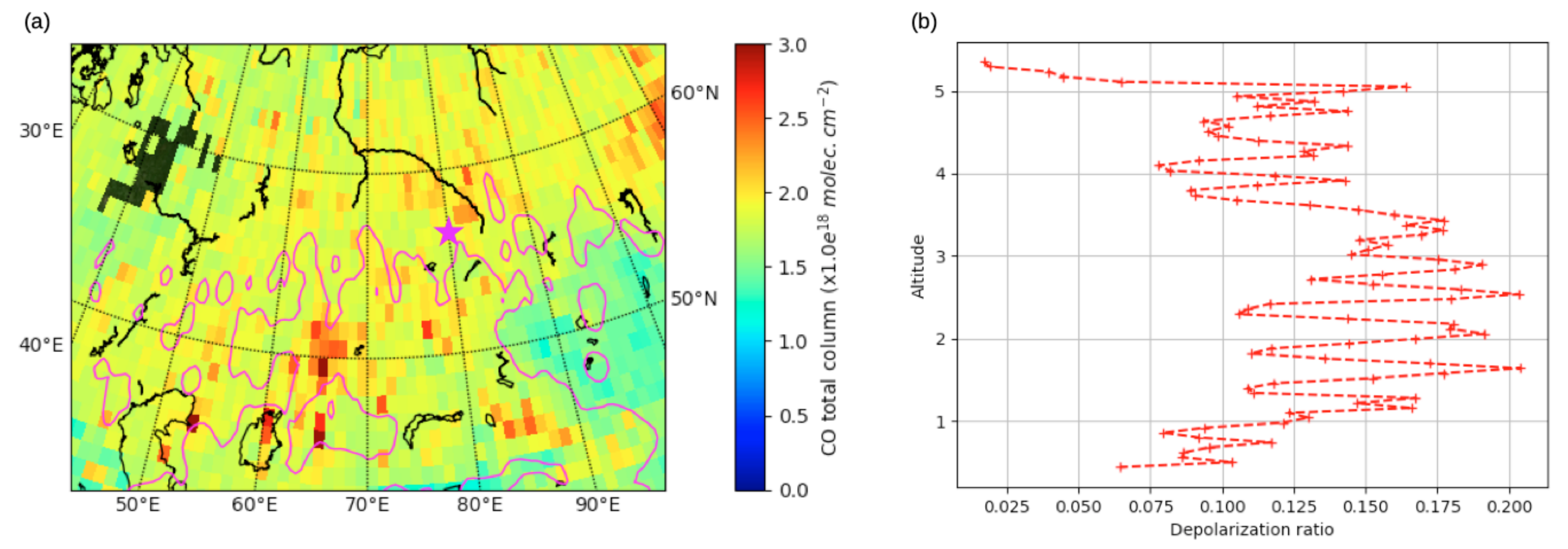
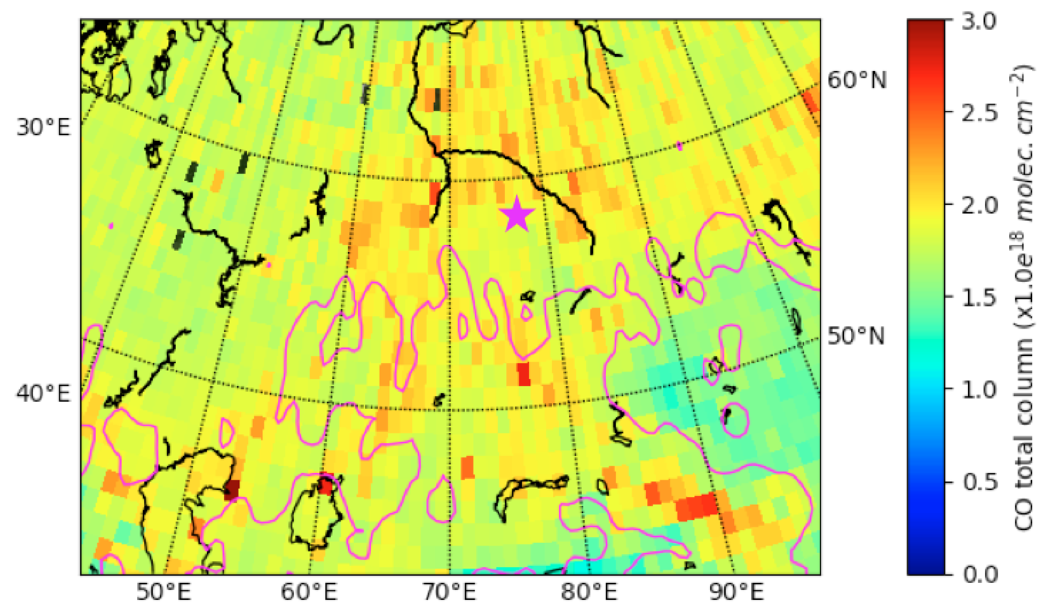
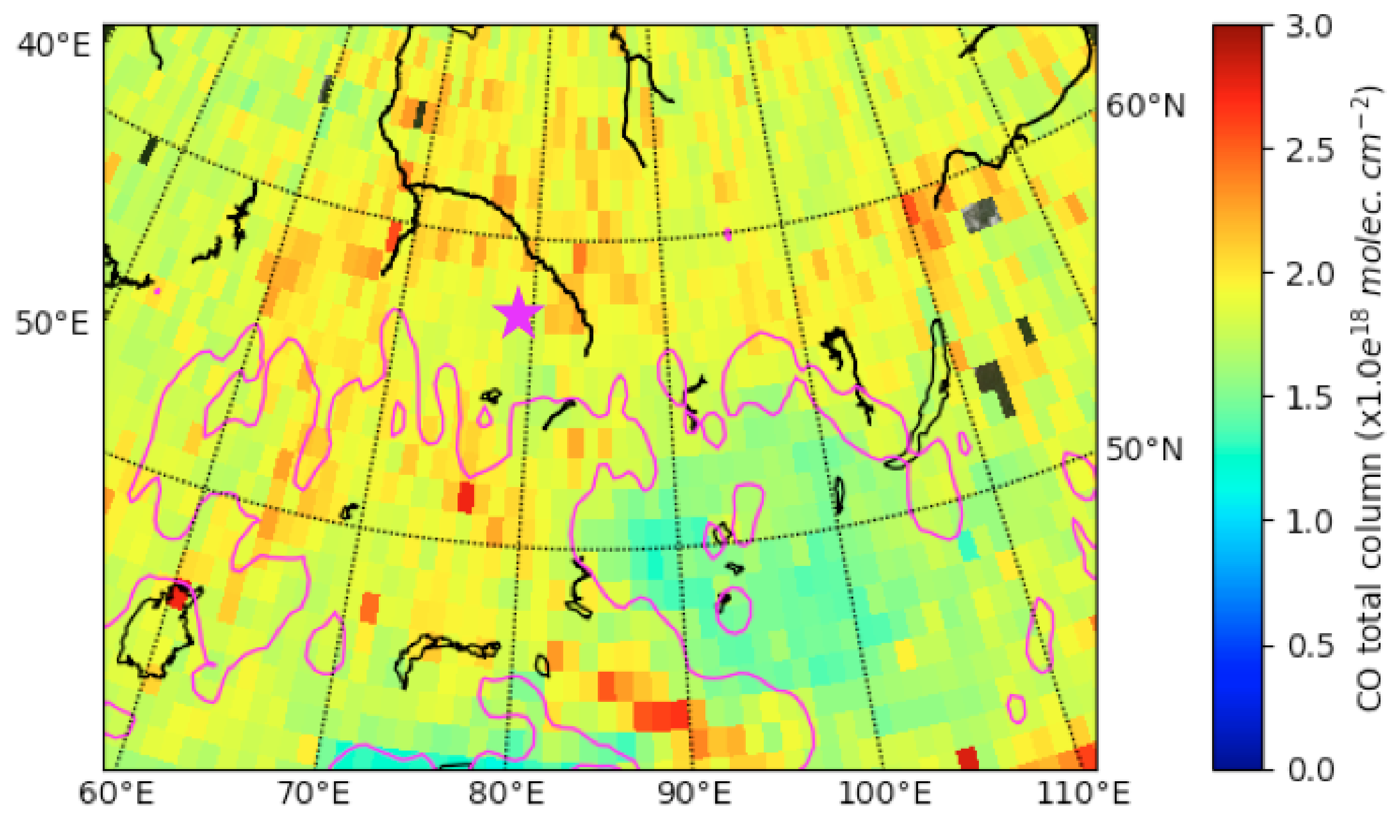
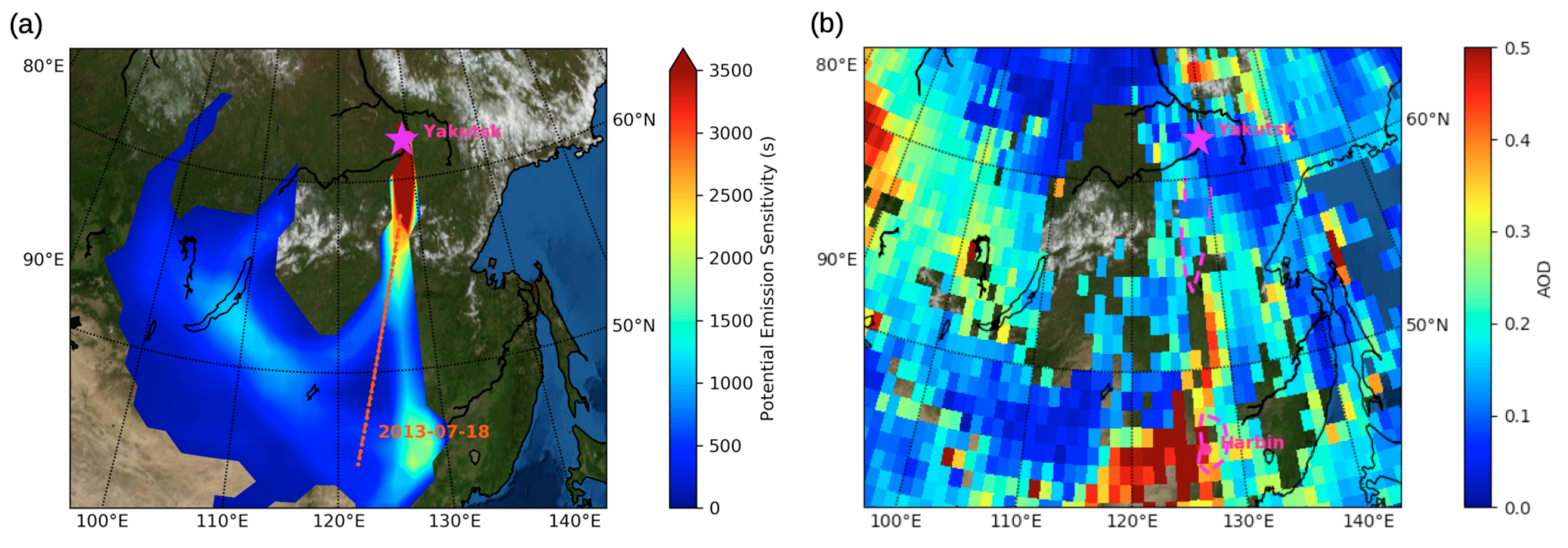
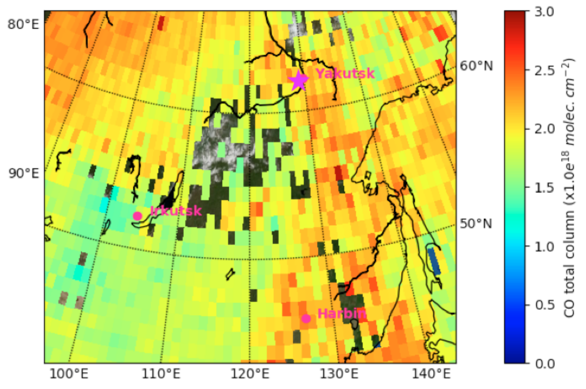
4.6. Long Range Transport of Northern China Emissions

The last case study corresponds to the lidar observations near the city of Yakutsk (62${}^{°}$ N, 129${}^{°}$ E) on 19 July 2013 at 11 UT. A PR2 vertical cross-section when slowly ascending west of Yakutsk shows several aerosol layers in the 0 and 5 km altitude range (Figure 22a).

The PES calculated by FLEXPART for the aerosol layer above 2 km and the MODIS AOD${}_{550}$ 4-day map show that the aerosol source region is located in a North–South corridor at 128${}^{°}$ E extending southward to the city of Harbin in Northern China (Figure 23). A smaller PES threshold of 2000 s has been chosen to define the source region for this layer because of significant removal of the aerosol tracer by washout during the transport from Northern China. The CO tropospheric column measured by IASI is also high (≥2.2 × 10${}^{18}$ molecule.cm${}^{-2}$) in the PES maximum at 45${}^{°}$ N, 128${}^{°}$ E (Figure 24). No fire is detected by FIRMS and no dust layer is seen by the AOD_{10$\mathsf{\mu }$m} measured by IASI in the area between Harbin and Yakutsk (Figure 24). Therefore, the main source of the aerosol layers observed by the lidar, and in particular the one located at altitude between 2.5 and 4 km, can be attributed to emissions from the Harbin region.

The $\mathsf{\Delta }$CO concentration measured by the aircraft during an ascent west of Yakutsk at 128.6${}^{°}$ E is as large as 75 ppbv in the layer between 2 and 4 km, while the ratio N${}_{80-200}$/N${}_A$ (0.8–1.0) is characteristic of aged aerosol with (Figure 22). This is consistent with the hypothesis of atmospheric transport of a polluted aerosol plume from a remote aerosol source in Northern China. The BC mass concentrations are similar to the values encountered for the previous case (0.2 $\mathsf{\mu }\mathrm{g}.{\mathrm{m}}^{-3}$) when flying around the Siberian cities. So either the contributions of Harbin and of Novosibirsk/Tomsk emissions to the BC atmospheric concentrations are similar or BC from Harbin emissions has been efficiently removed during the 2-day transport between Harbin and Yakutsk. AOD${}_{550}$ in the Harbin region remains high from 16 to 19 July 2013, therefore little changes are expected in the amount of aerosol emissions from this region.

The AOD${}_{532}$ and backscatter ratio profile are calculated for a 40 s average profile shown by the red rectangle in Figure 22 when the aircraft is high enough to sample the entire aerosol layer between 0 and 4 km. We could keep the same lidar ratio range considered in Section 4.5 for aerosol from Siberian cities, i.e., 43–90 sr. The backscatter ratio is again of the order of 2.2 in the layer near 3 km where the large $\mathsf{\Delta }$CO is measured. The AOD${}_{532}$ for the airborne lidar is then 0.19 ± 0.1 (Table 1). Because of the cloud cover in the southerly flow from Northern China on 17 and 18 July 2013, the number of MODIS AOD${}_{550}$ measurements is very small and only MODIS AOD${}_{550}$ average for a ±24 h time period is available (0.127 ± 0.04). The low AOD${}_{550}$ compared to the summer AOD${}_{550}$ values >0.4 usually encountered in Northern China [68] can be explained by the efficient aerosol removal in the southerly flow as shown also by the low BC concentrations measured by the aircraft. A CALIOP overpass on 18 July 2013 at 18 UT is perfectly located above the axis between Harbin and Yakutsk. A backscatter ratio vertical profile can be derived at 57${}^{°}$ N 12 h before the aircraft flight in Yakutsk and also shows an aerosol layer at 2.5 km above the PBL with a backscatter ratio of 2.3 similar to the measurements of the airborne lidar (Figure 25).

The CALIOP depolarization ratio is small (<5%) and the color ratio is of the order of 0.6 in this layer (Figure 25), i.e., as high as the value obtained in the polluted plume from the Siberian cities (Figure 21) but higher than the color ratio measured above the gas flaring area (Figure 10). High color ratio is expected for this case study considering the aerosol aging and the increase of the coarse size fraction during the long range transport of polluted aerosol from Northern China [69]. The CALIOP aerosol classification is in good agreement with the FLEXPART analysis with 68% of “Polluted Continental” layers and 32% of elevated smoke, while the corresponding LR (70 sr) and AOD${}_{532}$ (0.2 ± 0.07) is close to the aircraft observations 12 h later above Yakutsk.

5. Discussion

The characteristics of the six aerosol layers studied in this work are grouped in a summary table (Table 1). The dust/smoke layer transported from Kazakhstan and the aged smoke from Siberian fires have the lowest vertical extent (<2 km) with a nearly constant backscatter ratio of the order of 2. The limited vertical extent of the aged fire plumes have been already discussed in [13] using 2 years of lidar observations in Tomsk. On the contrary the vertical structure of fresh smoke plume shows a top altitude above 3.5 km and a well defined layer in the altitude range 2–4 km. The structure of urban plume from Northern China also shows a well defined layer in the same altitude range which can be explained by the upward transport in the frontal system along the West Pacific Coast. The two cases corresponding to urban and gas flaring plumes observed close to the emission area have a vertical extent of the order of 3 km and stronger vertical mixing between the ground and top altitude than for the fresh smoke and the urban plume transported from China. The meridional position of the plume east of 110${}^{°}$ E in the synoptic southerly flow from Northern China and the proximity of a fresh fire are then the main factors to explain the formation of well defined aerosol layers above 2 km above Siberia. The maximum backscatter ratio (3.5) is found for the fresh fire plumes while it is of the order of 2 for all other cases.

Using either lidar AOD${}_{532}$ (CALIOP and aircraft) or MODIS AOD${}_{550}$ the smallest aerosol extinction (AOD${}_{532}$< 0.15) were obtained for the dusty mix and fresh smoke, while the largest (AOD${}_{532}$≥ 0.2) are for the measurements on one hand above the gas flaring area in accordance with several studies on the impact of these emissions on aerosol production [5,70], and on the other hand for the long range transport of pollution [68]. It is worth mentioning that despite the large backscatter ratio for the fresh fire plume, the AOD${}_{532}$ remains below 0.15. Increase of the lidar ratio at 532 nm due to aging of the aerosol and mixing of many individual fire plumes explain the 40% increase of the AOD${}_{532}$ for the aged fire plume [14,57]. The largest differences between MODIS and lidar AOD are found for fresh plumes nearby the emission area (fire or urban pollution) where it becomes very important to take into account the measurement location mismatches. As explained in Section 4.2, the good agreement found between CALIOP and MODIS for the gas flaring case means that the lidar ratio range is probably 50–60 sr for the gas flaring plume sampled above Siberia.

Looking at the in-situ aircraft measurements, $\mathsf{\Delta }$CO increases for aged aerosol layers due to the long range transport of a biomass burning plume from Siberian fires or a polluted plume from Northern China. It is consistent with the CO lifetime being longer than 15 days and the buildup with time of individual plumes during the transport at regional scale [71,72]. BC mass concentration is high (>1.5 $\mathsf{\mu }$g.m${}^{-3}$) for the fresh biomass burning plume while it is less than 0.5 $\mathsf{\mu }$g.m${}^{-3}$ for the aged fire case because of efficient BC removal for transport lifetime > 1–2 days [59,60]. Gas flaring contribution to BC mass concentration (0.4–0.5 $\mathsf{\mu }\mathrm{g}.{\mathrm{m}}^{-3}$) is also higher than the urban pollution contribution either from local sources or transported from Northern China (0.2 $\mathsf{\mu }\mathrm{g}.{\mathrm{m}}^{-3}$). Moderate BC emissions from the local emissions of Siberian cities was not really expected considering the high value of $\mathsf{\Delta }$CO. It could be explained by a reduced combustion of wood and coal for urban heating during summer.

The lowest N${}_{80-200}$/N${}_A$ ratios are obtained in the case of the fresh fire plumes (0.15) and the highest values in the case of the long distance transport of aerosol from China (0.8). In the case of aged fire plumes, local emissions from flares or urban pollution sources, the N${}_{80-200}$/N${}_A$ ratio is between 0.3 and 0.6. Compared to the plume above the flares (ratio of 0.45 ± 0.15), aerosols in the aged fire plume (ratio of 0.6) probably have a significant fraction of terrigenous aerosol and exhibit an increase of the coarse size fraction due to coagulation during the transport from the source area [73,74]. The size spectrum measured by the DPS are shown in the supplementary document.

The color ratios from CALIOP observations are also consistent with the analysis of the N${}_{80-200}$/N${}_A$ ratios. The lowest CR values (0.2–0.4) are obtained for the fresh smoke and flaring cases while the dust/biomass mixture and aged smoke cases show values between 0.5 and 0.7. Usefulness of color ratio to quantify the coarse to fine aerosol fraction has already been proposed by [55]. The aerosol depolarization ratio values, derived from CALIOP observations, are low for all cases (<5%) except for fire plumes where a terrigenous aerosol fraction again seems likely.

On the whole, the aerosol type classification from CALIOP products is consistent with the FLEXPART analysis except for cases of flaring and aged fires for which a significant contribution of desert dust is proposed but not justified by the detailed study of the air mass transport. The 20% negative difference between AOD MODIS and AOD CALIOP for the aged fire plume indeed shows that a lidar ratio associated with the “Elevated Smoke” (70 sr) rather than “Polluted dust” (55 sr) could explain such a difference.

6. Conclusions

Two airborne lidar campaigns were carried out over Siberia in July 2013 and June 2017. Aerosol types and optical properties were derived using FLEXPART aerosol tracer transport simulations and satellite data (MODIS, IASI and CALIOP). The aircraft in-situ measurements, mainly $\mathsf{\Delta }$CO and BC have been useful to validate the identification of the aerosol origin. Six aerosol types could be identified in this work: (i) Dusty aerosol mixture (ii) Ob valley gas flaring emission (iii) fresh forest fire (iv) aged forest fire (v) urban emissions over the Tomsk/Novosibirsk region (vi) long range transport of Northern China urban emission.

Aerosol plumes transported above the boundary layer have been only observed for the synoptic uplifting of Northern China emissions or vertical transport during forest fire plume. This study also allows comparisons between aged and fresh plumes for both the urban and forest fire emissions. The aged forest fire plume is characterized by an increase of AOD${}_{532}$ and of the aerosol particle size in accordance with similar studies conducted in biomass burning aging in North America and Southern Europe. $\mathsf{\Delta }$CO increase (+10 ppbv) and BC decrease (≈−0.8 $\mathsf{\mu }\mathrm{g}.{\mathrm{m}}^{-3}$) have been also observed for the the aged fire plume, due to the accumulation of many individual plumes at regional scale and due to the BC wet or dry deposition. Similar results have been found for the comparison between the aerosol layers due to fresh and aged urban emission, especially the $\mathsf{\Delta }$CO increase (+20 ppbv) and the particle size increase (N${}_{80-200}$/N${}_A$ ratio from 0.5 to 1 and CALIOP color ratio from 0.4 to 0.6).

The flight above gas flaring emissions has been useful to discuss the characteristics of these plumes which have not been very well studied by aircraft lidar observations. The largest AOD is found for this air mass type regardless of the kind of observations (aircraft, CALIOP, MODIS). A range of 50–60 sr is proposed for the lidar ratio in aerosol plumes related to Siberian gas flaring emission based on the good agreement between the AOD retrieved by CALIOP and MODIS. Black carbon concentrations are relatively higher for the flaring plume (0.4–0.5 $\mathsf{\mu }\mathrm{g}.{\mathrm{m}}^{-3}$) than for the urban plume (0.2 $\mathsf{\mu }\mathrm{g}.{\mathrm{m}}^{-3}$). Based on the analysis of the color ratio and the N${}_{80-200}$/N${}_A$ ratio, the particle size in the flaring plume is slightly smaller than the aerosol size in the urban plume near Novosibirsk.

The aerosol type identification and AOD${}_{532}$ provided by CALIOP Version 4.2 data products in air masses with similar origin generally agrees with the results obtained with our analysis of the aerosol plume origin, except for the flaring and aged fire layers where a significant contribution of dust is not justified. The CALIOP derived color ratio is also in good agreement with the behavior of the N${}_{80-200}$/N${}_A$ ratio measured by the aircraft aerosol size distribution measurements. Such results are important considering the large amount of CALIOP observations available to characterize the optical properties over Siberia.

References

1. Chỳlek, P.; Coakley, J.A. Aerosols and climate. Science 1974, 183, 75–77. [Google Scholar]
2. Stocker, T.F.; Qin, D.; Plattner, G.K.; Tignor, M.; Allen, S.K.; Boschung, J.; Nauels, A.; Xia, Y.; Bex, V.; Midgley, P.M. Climate Change 2013: The Physical Science Basis. Contribution of Working Group I to the Fifth Assessment Report of IPCC the Intergovernmental Panel on Climate Change; Cambridge University Press: Cambridge, UK, 2014. [Google Scholar] [CrossRef] [Green Version]
3. Lavoué, D.; Liousse, C.; Cachier, H.; Stocks, B.J.; Goldammer, J.G. Modeling of carbonaceous particles emitted by boreal and temperate wildfires at northern latitudes. J. Geophys. Res. Atmos. 2000, 105, 26871–26890. [Google Scholar] [CrossRef] [Green Version]
4. Paris, J.D.; Stohl, A.; Nédélec, P.; Arshinov, M.Y.; Panchenko, M.; Shmargunov, V.; Law, K.S.; Belan, B.; Ciais, P. Wildfire smoke in the Siberian Arctic in summer: Source characterization and plume evolution from airborne measurements. Atmos. Chem. Phys. 2009, 9, 9315–9327. [Google Scholar] [CrossRef] [Green Version]
5. Stohl, A.; Klimont, Z.; Eckhardt, S.; Kupiainen, K.; Shevchenko, V.P.; Kopeikin, V.; Novigatsky, A. Black carbon in the Arctic: The underestimated role of gas flaring and residential combustion emissions. Atmos. Chem. Phys. 2013, 13, 8833–8855. [Google Scholar] [CrossRef] [Green Version]
6. Bond, T.C.; Doherty, S.J.; Fahey, D.; Forster, P.; Berntsen, T.; DeAngelo, B.; Flanner, M.; Ghan, S.; Kärcher, B.; Koch, D.; et al. Bounding the role of black carbon in the climate system: A scientific assessment. J. Geophys. Res. Atmos. 2013, 118, 5380–5552. [Google Scholar] [CrossRef]
7. Huang, K.; Fu, J.S.; Prikhodko, V.Y.; Storey, J.M.; Romanov, A.; Hodson, E.L.; Cresko, J.; Morozova, I.; Ignatieva, Y.; Cabaniss, J. Russian anthropogenic black carbon: Emission reconstruction and Arctic black carbon simulation. J. Geophys. Res. Atmos. 2015. [Google Scholar] [CrossRef]
8. Paris, J.D.; Ciais, P.; Nédélec, P.; Ramonet, M.; Belan, B.; Arshinov, M.Y.; Golitsyn, G.; Granberg, I.; Stohl, A.; Cayez, G.; et al. The YAK-AEROSIB transcontinental aircraft campaigns: New insights on the transport of CO2, CO and O3 across Siberia. Tellus B Chem. Phys. Meteorol. 2008, 60, 551–568. [Google Scholar] [CrossRef] [Green Version]
9. Paris, J.D.; Arshinov, M.Y.; Ciais, P.; Belan, B.D.; Nedelec, P. Large-scale aircraft observations of ultra-fine and fine particle concentrations in the remote Siberian troposphere: New particle formation studies. Atmos. Environ. 2009, 43, 1302–1309. [Google Scholar] [CrossRef]
10. Dieudonné, E.; Chazette, P.; Marnas, F.; Totems, J.; Shang, X. Lidar profiling of aerosol optical properties from Paris to Lake Baikal (Siberia). Atmos. Chem. Phys. 2015, 15, 5007–5026. [Google Scholar] [CrossRef] [Green Version]
11. Samoilova, S.; Balin, Y.S.; Kokhanenko, G.; Penner, I. Investigation of the vertical distribution of tropospheric aerosol layers from multifrequency laser sensing data. Part 2: The vertical distribution of optical aerosol characteristics in the visible region. Atmos. Ocean. Opt. 2010, 23, 95–105. [Google Scholar] [CrossRef]
12. Samoilova, S.; Balin, Y.S.; Kokhanenko, G.; Penner, I. Investigation of the vertical distribution of tropospheric aerosol layers using the data of multiwavelength lidar sensing. Part 3. Spectral peculiarities of the vertical distribution of the aerosol optical characteristics. Atmos. Ocean. Opt. 2012, 25, 208–215. [Google Scholar] [CrossRef]
13. Ancellet, G.; Penner, I.E.; Pelon, J.; Mariage, V.; Zabukovec, A.; Raut, J.C.; Kokhanenko, G.; Balin, Y.S. Aerosol monitoring in Siberia using an 808 nm automatic compact lidar. Atmos. Meas. Tech. 2019, 12, 147–168. [Google Scholar] [CrossRef] [Green Version]
14. Burton, S.; Ferrare, R.; Hostetler, C.; Hair, J.; Rogers, R.; Obland, M.; Butler, C.; Cook, A.; Harper, D.; Froyd, K. Aerosol classification using airborne High Spectral Resolution Lidar measurements–methodology and examples. Atmos. Meas. Tech. 2012, 5, 73–98. [Google Scholar] [CrossRef] [Green Version]
15. Burton, S.; Ferrare, R.; Vaughan, M.; Omar, A.; Rogers, R.; Hostetler, C.; Hair, J. Aerosol classification from airborne HSRL and comparisons with the CALIPSO vertical feature mask. Atmos. Meas. Tech. 2013, 6, 1397–1412. [Google Scholar] [CrossRef] [Green Version]
16. Groß, S.; Esselborn, M.; Weinzierl, B.; Wirth, M.; Fix, A.; Petzold, A. Aerosol classification by airborne high spectral resolution lidar observations. Atmos. Chem. Phys. 2013, 13, 2487–2505. [Google Scholar] [CrossRef] [Green Version]
17. Pelon, J.; Flamant, C.; Chazette, P.; Leon, J.F.; Tanré, D.; Sicard, M.; Satheesh, S. Characterization of aerosol spatial distribution and optical properties over the Indian Ocean from airborne LIDAR and radiometry during INDOEX’99. J. Geophys. Res. Atmos. 2002, 107, INX2-28. [Google Scholar] [CrossRef] [Green Version]
18. Winker, D.M.; Vaughan, M.A.; Omar, A.; Hu, Y.; Powell, K.A.; Liu, Z.; Hunt, W.H.; Young, S.A. Overview of the CALIPSO mission and CALIOP data processing algorithms. J. Atmos. Ocean. Technol. 2009, 26, 2310–2323. [Google Scholar] [CrossRef]
19. Pierro, M.D.; Jaeglé, L.; Anderson, T. Satellite observations of aerosol transport from East Asia to the Arctic: Three case studies. Atmos. Chem. Phys. 2011, 11, 2225–2243. [Google Scholar] [CrossRef] [Green Version]
20. Devasthale, A.; Tjernström, M.; Omar, A.H. The vertical distribution of thin features over the Arctic analysed from CALIPSO observations: Part II: Aerosols. Tellus B Chem. Phys. Meteorol. 2011, 63, 86–95. [Google Scholar] [CrossRef] [Green Version]
21. Ancellet, G.; Pelon, J.; Blanchard, Y.; Quennehen, B.; Bazureau, A.; Law, K.S.; Schwarzenboeck, A. Transport of aerosol to the Arctic: Analysis of CALIOP and French aircraft data during the spring 2008 POLARCAT campaign. Atmos. Chem. Phys. 2014, 14, 8235–8254. [Google Scholar] [CrossRef] [Green Version]
22. Di Biagio, C.; Pelon, J.; Ancellet, G.; Bazureau, A.; Mariage, V. Sources, Load, Vertical Distribution, and Fate of Wintertime Aerosols North of Svalbard From Combined V4 CALIOP Data, Ground-Based IAOOS Lidar Observations and Trajectory Analysis. J. Geophys. Res. Atmos. 2018, 123, 1363–1383. [Google Scholar] [CrossRef]
23. Omar, A.H.; Winker, D.M.; Vaughan, M.A.; Hu, Y.; Trepte, C.R.; Ferrare, R.A.; Lee, K.P.; Hostetler, C.A.; Kittaka, C.; Rogers, R.R.; et al. The CALIPSO automated aerosol classification and lidar ratio selection algorithm. J. Atmos. Ocean. Technol. 2009, 26, 1994–2014. [Google Scholar] [CrossRef]
24. Kim, M.H.; Omar, A.H.; Tackett, J.L.; Vaughan, M.A.; Winker, D.M.; Trepte, C.R.; Hu, Y.; Liu, Z.; Poole, L.R.; Pitts, M.C.; et al. The CALIPSO version 4 automated aerosol classification and lidar ratio selection algorithm. Atmos. Meas. Tech. 2018, 11, 6107–6135. [Google Scholar] [CrossRef] [Green Version]
25. Müller, D.; Ansmann, A.; Mattis, I.; Tesche, M.; Wandinger, U.; Althausen, D.; Pisani, G. Aerosol-type-dependent lidar ratios observed with Raman lidar. J. Geophys. Res. Atmos. 2007, 112. [Google Scholar] [CrossRef]
26. Balin, Y.; Bairashin, G.; Kokhanenko, G.; Penner, I.; Samoilova, S. LOSA-M2 aerosol Raman lidar. Quantum Electron. 2011, 41, 945. [Google Scholar] [CrossRef]
27. Penner, I.E.; Balin, Y.S.; Kokhanenko, G.P.; Belan, B.D.; Arshinov, M.Y.; Chernov, D.G.; Kozlov, V.S. Detection of aerosol plumes from associated gas flaring by laser sensing. In 21st International Symposium Atmospheric and Ocean Optics: Atmospheric Physics; Romanovskii, O.A., Ed.; International Society for Optics and Photonics, SPIE: Bellingham, WA, USA, 2015; Volume 9680, pp. 919–923. [Google Scholar] [CrossRef]
28. Nedelec, P.; Cammas, J.P.; Thouret, V.; Athier, G.; Cousin, J.M.; Legrand, C.; Abonnel, C.; Lecoeur, F.; Cayez, G.; Marizy, C. An improved infrared carbon monoxide analyser for routine measurements aboard commercial Airbus aircraft: Technical validation and first scientific results of the MOZAIC III programme. Atmos. Chem. Phys. Discuss. 2003, 3, 3713–3744. [Google Scholar] [CrossRef] [Green Version]
29. Panchenko, M.; Kozlov, V.; Terpugova, S.; Shmargunov, V.; Burkov, V.; Simultaneous measurements of submicron aerosol and absorbing substance in the height range up to 7 km. In Tenth ARM Science Team Meeting Proceeding, San Antonio, TX, USA, 13–17 March 2000; pp. 13–17. Available online: https://armweb0-stg.ornl.gov/publications/proceedings/conf10/extended_abs/panchenko_mv.pdf (accessed on 3 February 2021).
30. Ankilow, A.; Baklanov, A.; Mavliev, R.; Eremenko, S.; Reischl, G.; Majerowicz, A. Comparison ofthe Novosibirsk automated diffusion battery with the Vienna electro mobility spectrometer. J. Aerosol Sci. 1991, 22, S325–S328. [Google Scholar] [CrossRef]
31. Ankilov, A.; Baklanov, A.; Colhoun, M.; Enderle, K.H.; Gras, J.; Julanov, Y.; Kaller, D.; Lindner, A.; Lushnikov, A.; Mavliev, R.; et al. Particle size dependent response of aerosol counters. Atmos. Res. 2002, 62, 209–237. [Google Scholar] [CrossRef]
32. Ankilov, A.; Baklanov, A.; Colhoun, M.; Enderle, K.H.; Gras, J.; Julanov, Y.; Kaller, D.; Lindner, A.; Lushnikov, A.; Mavliev, R.; et al. Intercomparison of number concentration measurements by various aerosol particle counters. Atmos. Res. 2002, 62, 177–207. [Google Scholar] [CrossRef]
33. Fernald, F.G. Analysis of atmospheric lidar observations: Some comments. Appl. Opt. 1984, 23, 652–653. [Google Scholar] [CrossRef] [PubMed]
34. Dee, D.P.; Uppala, S.M.; Simmons, A.; Berrisford, P.; Poli, P.; Kobayashi, S.; Andrae, U.; Balmaseda, M.; Balsamo, G.; Bauer, D.P.; et al. The ERA-Interim reanalysis: Configuration and performance of the data assimilation system. Q. J. R. Meteorol. Soc. 2011, 137, 553–597. [Google Scholar] [CrossRef]
35. Stohl, A.; Seibert, P. Accuracy of trajectories as determined from the conservation of meteorological tracers. Q. J. R. Meteorol. Soc. 1998, 124, 1465–1484. [Google Scholar] [CrossRef]
36. Stohl, A.; Eckhardt, S.; Forster, C.; James, P.; Spichtinger, N.; Seibert, P. A replacement for simple back trajectory calculations in the interpretation of atmospheric trace substance measurements. Atmos. Environ. 2002, 36, 4635–4648. [Google Scholar] [CrossRef]
37. Seibert, P.; Frank, A. Source-receptor matrix calculation with a Lagrangian particle dispersion model in backward mode. Atmos. Chem. Phys. 2004, 4, 51–63. [Google Scholar] [CrossRef] [Green Version]
38. Giglio, L.; Descloitres, J.; Justice, C.O.; Kaufman, Y.J. An enhanced contextual fire detection algorithm for MODIS. Remote Sens. Environ. 2003, 87, 273–282. [Google Scholar] [CrossRef]
39. Schroeder, W.; Oliva, P.; Giglio, L.; Csiszar, I.A. The New VIIRS 375 m active fire detection data product: Algorithm description and initial assessment. Remote Sens. Environ. 2014, 143, 85–96. [Google Scholar] [CrossRef]
40. Clerbaux, C.; Chazette, P.; Hadji-Lazaro, J.; Mégie, G.; Müller, J.F.; Clough, S. Remote sensing of CO, CH4, and O3 using a spaceborne nadir-viewing interferometer. J. Geophys. Res. Atmos. 1998, 103, 18999–19013. [Google Scholar] [CrossRef]
41. Hadji-Lazaro, J.; Clerbaux, C.; Thiria, S. An inversion algorithm using neural networks to retrieve atmospheric CO total columns from high-resolution nadir radiances. J. Geophys. Res. Atmos. 1999, 104, 23841–23854. [Google Scholar] [CrossRef] [Green Version]
42. Hurtmans, D.; Coheur, P.F.; Wespes, C.; Clarisse, L.; Scharf, O.; Clerbaux, C.; Hadji-Lazaro, J.; George, M.; Turquety, S. FORLI radiative transfer and retrieval code for IASI. J. Quant. Spectrosc. Radiat. Transf. 2012, 113, 1391–1408. [Google Scholar] [CrossRef]
43. Clerbaux, C. Daily IASI/Metop-A ULB-LATMOS Carbon Monoxide (CO) L2 Product (Total Column). 2018. Available online: https://doi.org.10.25326/16 (accessed on 3 February 2021).
44. Peyridieu, S.; Chédin, A.; Capelle, V.; Tsamalis, C.; Pierangelo, C.; Armante, R.; Crevoisier, C.; Crépeau, L.; Siméon, M.; Ducos, F.; et al. Characterisation of dust aerosols in the infrared from IASI and comparison with PARASOL, MODIS, MISR, CALIOP, and AERONET observations. Atmos. Chem. Phys. 2013, 13, 6065–6082. [Google Scholar] [CrossRef] [Green Version]
45. Capelle, V.; Chédin, A.; Siméon, M.; Tsamalis, C.; Pierangelo, C.; Pondrom, M.; Armante, R.; Crevoisier, C.; Crepeau, L.; Scott, N. Evaluation of IASI derived dust aerosols characteristics over the tropical belt. Atmos. Chem. Phys. Discuss. 2013, 13. [Google Scholar] [CrossRef] [Green Version]
46. Capelle, V.; Chédin, A.; Pondrom, M.; Crevoisier, C.; Armante, R.; Crepeau, L.; Scott, N. Infrared dust aerosol optical depth retrieved daily from IASI and comparison with AERONET over the period 2007–2016. Remote Sens. Environ. 2018, 206, 15–32. [Google Scholar] [CrossRef]
47. Tesche, M.; Gross, S.; Ansmann, A.; Mueller, D.; Althausen, D.; Freudenthaler, V.; Esselborn, M. Profiling of Saharan dust and biomass-burning smoke with multiwavelength polarization Raman lidar at Cape Verde. Tellus B Chem. Phys. Meteorol. 2011, 63, 649–676. [Google Scholar] [CrossRef] [Green Version]
48. Groß, S.; Tesche, M.; Freudenthaler, V.; Toledano, C.; Wiegner, M.; Ansmann, A.; Althausen, D.; Seefeldner, M. Characterization of Saharan dust, marine aerosols and mixtures of biomass-burning aerosols and dust by means of multi-wavelength depolarization and Raman lidar measurements during SAMUM 2. Tellus B Chem. Phys. Meteorol. 2011, 63, 706–724. [Google Scholar] [CrossRef]
49. Klimont, Z.; Kupiainen, K.; Heyes, C.; Purohit, P.; Cofala, J.; Rafaj, P.; Borken-Kleefeld, J.; Schöpp, W. Global anthropogenic emissions of particulate matter including black carbon. Atmos. Chem. Phys. 2017, 17, 8681–8723. [Google Scholar] [CrossRef] [Green Version]
50. Wang, P.; Elansky, N.; Timofeev, Y.M.; Wang, G.; Golitsyn, G.; Makarova, M.; Rakitin, V.; Shtabkin, Y.; Skorokhod, A.; Grechko, E.; et al. Long-Term Trends of Carbon Monoxide Total Columnar Amount in Urban Areas and Background Regions: Ground-and Satellite-based Spectroscopic Measurements. Adv. Atmos. Sci. 2018, 35, 785–795. [Google Scholar] [CrossRef]
51. Willeke, K.; Whitby, K.T. Atmospheric aerosols: Size distribution interpretation. J. Air Pollut. Control Assoc. 1975, 25, 529–534. [Google Scholar] [CrossRef]
52. Bäumer, D.; Vogel, B.; Versick, S.; Rinke, R.; Möhler, O.; Schnaiter, M. Relationship of visibility, aerosol optical thickness and aerosol size distribution in an ageing air mass over South-West Germany. Atmos. Environ. 2008, 42, 989–998. [Google Scholar] [CrossRef]
53. Furutani, H.; Dall’osto, M.; Roberts, G.C.; Prather, K.A. Assessment of the relative importance of atmospheric aging on CCN activity derived from field observations. Atmos. Environ. 2008, 42, 3130–3142. [Google Scholar] [CrossRef]
54. Tesche, M.; Ansmann, A.; Müller, D.; Althausen, D.; Engelmann, R.; Hu, M.; Zhang, Y. Particle backscatter, extinction, and lidar ratio profiling with Raman lidar in south and north China. Appl. Opt. 2007, 46, 6302–6308. [Google Scholar] [CrossRef] [PubMed]
55. De Villiers, R.A.; Ancellet, G.; Pelon, J.; Quennehen, B.; Schwarzenboeck, A.; Gayet, J.F.; Law, K.S. Airborne measurements of aerosol optical properties related to early spring transport of mid-latitude sources into the Arctic. Atmos. Chem. Phys. 2010, 10, 5011–5030. [Google Scholar] [CrossRef] [Green Version]
56. Chazette, P.; Raut, J.C.; Totems, J. Springtime aerosol load as observed from ground-based and airborne lidars over northern Norway. Atmos. Chem. Phys. 2018, 18, 13075–13095. [Google Scholar] [CrossRef] [Green Version]
57. Nicolae, D.; Nemuc, A.; Mueller, D.; Talianu, C.; Vasilescu, J.; Belegante, L.; Kolgotin, A. Characterization of fresh and aged biomass burning events using multiwavelength Raman lidar and mass spectrometry. J. Geophys. Res. Atmos. 2013, 118, 2956–2965. [Google Scholar] [CrossRef]
58. Müller, D.; Mattis, I.; Wandinger, U.; Ansmann, A.; Althausen, D.; Stohl, A. Raman lidar observations of aged Siberian and Canadian forest fire smoke in the free troposphere over Germany in 2003: Microphysical particle characterization. J. Geophys. Res. Atmos. 2005, 110. [Google Scholar] [CrossRef]
59. Cape, J.; Coyle, M.; Dumitrean, P. The atmospheric lifetime of black carbon. Atmos. Environ. 2012, 59, 256–263. [Google Scholar] [CrossRef] [Green Version]
60. Lund, M.T.; Samset, B.H.; Skeie, R.B.; Watson-Parris, D.; Katich, J.M.; Schwarz, J.P.; Weinzierl, B. Short Black Carbon lifetime inferred from a global set of aircraft observations. Npj Clim. Atmos. Sci. 2018, 1, 31. [Google Scholar] [CrossRef]
61. Murayama, T.; Müller, D.; Wada, K.; Shimizu, A.; Sekiguchi, M.; Tsukamoto, T. Characterization of Asian dust and Siberian smoke with multi-wavelength Raman lidar over Tokyo, Japan in spring 2003. Geophys. Res. Lett. 2004, 31. [Google Scholar] [CrossRef] [Green Version]
62. Noh, Y.M.; Kim, Y.J.; Müller, D. Seasonal characteristics of lidar ratios measured with a Raman lidar at Gwangju, Korea in spring and autumn. Atmos. Environ. 2008, 42, 2208–2224. [Google Scholar] [CrossRef]
63. Xie, C.; Nishizawa, T.; Sugimoto, N.; Matsui, I.; Wang, Z. Characteristics of aerosol optical properties in pollution and Asian dust episodes over Beijing, China. Appl. Opt. 2008, 47, 4945–4951. [Google Scholar] [CrossRef]
64. Ansmann, A.; Engelmann, R.; Althausen, D.; Wandinger, U.; Hu, M.; Zhang, Y.; He, Q. High aerosol load over the Pearl River Delta, China, observed with Raman lidar and Sun photometer. Geophys. Res. Lett. 2005, 32. [Google Scholar] [CrossRef]
65. Heese, B.; Baars, H.; Bohlmann, S.; Althausen, D.; Deng, R. Continuous vertical aerosol profiling with a multi-wavelength Raman polarization lidar over the Pearl River Delta, China. Atmos. Chem. Phys. 2017, 17, 6679–6691. [Google Scholar] [CrossRef] [Green Version]
66. Dieudonné, E.; Chazette, P.; Marnas, F.; Totems, J.; Shang, X. Raman Lidar Observations of Aerosol Optical Properties in 11 Cities from France to Siberia. Remote Sens. 2017, 9, 978. [Google Scholar] [CrossRef] [Green Version]
67. Chazette, P.; Randriamiarisoa, H.; Sanak, J.; Couvert, P.; Flamant, C. Optical properties of urban aerosol from airborne and ground-based in situ measurements performed during the Etude et Simulation de la Qualité de l’air en Ile de France (ESQUIF) program. J. Geophys. Res. Atmos. 2005, 110. [Google Scholar] [CrossRef] [Green Version]
68. Li, J.; Liu, R.; Liu, S.C.; Shiu, C.J.; Wang, J.; Zhang, Y. Trends in aerosol optical depth in northern China retrieved from sunshine duration data. Geophys. Res. Lett. 2016, 43, 431–439. [Google Scholar] [CrossRef] [Green Version]
69. Cheung, H.C.; Chou, C.C.K.; Lee, C.S.L.; Kuo, W.C.; Chang, S.C. Hygroscopic properties and cloud condensation nuclei activity of atmospheric aerosols under the influences of Asian continental outflow and new particle formation at a coastal site in eastern Asia. Atmos. Chem. Phys. 2020, 20, 5911–5922. [Google Scholar] [CrossRef]
70. Elvidge, C.D.; Zhizhin, M.; Baugh, K.; Hsu, F.C.; Ghosh, T. Methods for Global Survey of Natural Gas Flaring from Visible Infrared Imaging Radiometer Suite Data. Energies 2016, 9, 14. [Google Scholar] [CrossRef]
71. Forster, C.; Wandinger, U.; Wotawa, G.; James, P.; Mattis, I.; Althausen, D.; Simmonds, P.; O’Doherty, S.; Jennings, S.G.; Kleefeld, C.; et al. Transport of boreal forest fire emissions from Canada to Europe. J. Geophys. Res. Atmos. 2001, 106, 22887–22906. [Google Scholar] [CrossRef]
72. Petetin, H.; Sauvage, B.; Parrington, M.; Clark, H.; Fontaine, A.; Athier, G.; Blot, R.; Boulanger, D.; Cousin, J.M.; Nédélec, P.; et al. The role of biomass burning as derived from the tropospheric CO vertical profiles measured by IAGOS aircraft in 2002–2017. Atmos. Chem. Phys. 2018, 18, 17277–17306. [Google Scholar] [CrossRef] [Green Version]
73. Sakamoto, K.M.; Laing, J.R.; Stevens, R.G.; Jaffe, D.A.; Pierce, J.R. The evolution of biomass-burning aerosol size distributions due to coagulation: Dependence on fire and meteorological details and parameterization. Atmos. Chem. Phys. 2016, 16, 7709–7724. [Google Scholar] [CrossRef] [Green Version]
74. Quennehen, B.; Schwarzenboeck, A.; Matsuki, A.; Burkhart, J.F.; Stohl, A.; Ancellet, G.; Law, K.S. Anthropogenic and forest fire pollution aerosol transported to the Arctic: Observations from the POLARCAT-France spring campaign. Atmos. Chem. Phys. 2012, 12, 6437–6454. [Google Scholar] [CrossRef] [Green Version]
Figure 1. (a) Map of the 8 aircraft flight tracks carried out in 2013 (eastern loop) and in 2017 (northern loop). The aircraft altitude ranges in km ASL are also shown for the 2017 (b) and 2013 (c) flights. Each color corresponds to a given flight. The red and yellow flights in June 2017 are along the same track. Map background: NASA’s Earth Observatory.
Atmosphere 12 00244 g001
Figure 2. Flow chart of airborne lidar data processing and aerosol types identification.
Atmosphere 12 00244 g002
Figure 3. (a) Vertical cross-section of airborne lidar log 10 ( P R 2 ) on 16 June 2017 at 5 UT. Calibration constant is 13,458 ± 2%. Grimm aerosol concentrations in particle.cm 3 are shown at the aircraft altitude. (b) Vertical profiles of Δ CO in ppbv (grey), BC in μ g . m 3 (green) for the descent at 57.5 ° N. (c) Backscatter ratio vertical profile for the lidar data in the red box. The horizontal dotted line is the top of the aerosol layer according to the lidar data.
Atmosphere 12 00244 g003
Figure 4. (a) Map of the vertically integrated PES distribution in s from a FLEXPART backward simulation for the aerosol layer of Figure 3. Orange dotted lines are the CALIOP nighttime overpasses at 21 UT on 16 June (70 ° E) and 15 June (80 ° E), 2017. The yellow dotted circle is the dust source area. (b) Average of MODIS AOD 550 1 ° × 1 ° from 13 to 16 June 2017 with PES ≥ 2300 s shown by the pink dotted isoline. The aircraft position is shown by the pink star at 56.6 ° N (Map background: NASA’s Earth Observatory).
Atmosphere 12 00244 g004
Figure 5. (a) Average of IASI tropospheric CO total column (in 1.0 × 10 18 molecule . cm 2 ) from 13 to 16 June 2017. Pink isolines define areas with 10 μ m AOD > 0.08. The pink star is the aircraft position on 16 June 2017. (b) CALIOP 532 nm particle linear depolarization ratio vertical profile in the aerosol source region at 49.7 ° N, 70 ° E (see Figure 4a).
Atmosphere 12 00244 g005
Figure 6. (a) Vertical profiles of 532 nm backscatter ratio for the aircraft lidar in red box of Figure 3a (red line) and for CALIOP on 15 June 2017 at 21 UT and 54 ° N, 75 ° E. (blue line), (b) Vertical profiles of the particle color ratio (green) and particle linear depolarization ratio (red) measured by CALIOP.
Atmosphere 12 00244 g006
Figure 7. (a) Vertical cross-section of airborne lidar log 10 ( P R 2 ) on 18 June 2017 at 01 UT. Calibration constant is 63413 ± 2%. Grimm aerosol concentrations in particle.cm 3 are shown at the aircraft altitude. (b) Vertical profiles of Δ CO in ppbv (grey), BC in μ g . m 3 (green) and ratio of N 80 200 /N A (blue dashed line) concentrations for the descent at 59 ° N. (c) Backscatter ratio vertical profile for the lidar data in the red box. The horizontal dotted line is the top of the aerosol layer according to the lidar data.
Atmosphere 12 00244 g007
Figure 8. (a) as Figure 4a for the aerosol layer of Figure 7. Orange dotted line is the position of the CALIOP overpass on 18 June 2017. (b) as Figure 4b with averaging of MODIS AOD 550 from 15 to 18 June 2017.
Atmosphere 12 00244 g008
Figure 9. As Figure 5a for the time period 13–16 June 2017.
Atmosphere 12 00244 g009
Figure 10. (a) Vertical profiles of 532 nm backscatter ratio for the aircraft lidar in red box of Figure 7a (red line) and for CALIOP on 18 June 2017 at 21 UT and 57 ° N (blue line). (b) Vertical profiles of the particle color ratio (green) and particle linear depolarization ratio (red) measured by CALIOP.
Atmosphere 12 00244 g010
Figure 11. (a) Vertical cross-section of aircraft log 10 ( P R 2 ) on 19 July 2013 at 06 UT. Calibration constant is 491,724 ± 10%. Grimm aerosol concentrations in particle.cm 3 are shown at the aircraft altitude. (b) Vertical profiles of Δ CO in ppbv (grey), BC in μ g . m 3 (green) and ratio N 80 200 /N A (blue dashed line) for the descent at 94 ° E. (c) Backscatter ratio vertical profile for the lidar data in the red box.
Atmosphere 12 00244 g011
Figure 12. (a) as Figure 4a for the aerosol layer of Figure 11. Orange dotted lines are the positions of the two CALIOP overpasses on 16 and 18 July 2013. (b) as Figure 4b with averaging of MODIS AOD 550 from 16 to 19 July 2013.
Atmosphere 12 00244 g012
Figure 13. (a) Vertical profiles of 532 nm backscatter ratio for the aircraft lidar in red box of Figure 11a (red line) and for CALIOP on 16 and 18 July 2013 at, respectively 19 UT, 62 ° N and 05 UT, 59 ° N. (b) Vertical profiles of the particle color ratio (green) and particle linear depolarization ratio (red) measured by CALIOP.
Atmosphere 12 00244 g013
Figure 14. (a) Vertical cross-section of aircraft log 10 ( P R 2 ) on 18 June 2017, 03 UT. Calibration constant is 83014 ± 5%. Grimm aerosol concentrations in particle.cm 3 are shown at the aircraft altitude. (b) Vertical profiles of Δ CO in ppbv (grey), BC in μ g . m 3 (green) and ratio of N 80 200 /N A (blue dashed line) for the descent at 56 ° N. (c) Backscatter ratio vertical profile for the lidar data in the red box. The horizontal dotted line is the top of the aerosol layer according to the lidar data.
Atmosphere 12 00244 g014
Figure 15. (a) as Figure 4a for the aerosol layer of Figure 14. Orange dotted lines are the two CALIOP overpasses on 17 June 2017 at 6 UT and 19 UT. (b) as Figure 4b with averaging of MODIS AOD 550 from 15 to 18 June 2017.
Atmosphere 12 00244 g015
Figure 16. As Figure 5a for the time period 15–18 June 2017.
Atmosphere 12 00244 g016
Figure 17. (a) Vertical profiles of 532 nm backscatter ratio for the aircraft lidar in red box of Figure 14a (red line) and for CALIOP on 7 June 2017 at, respectively 6 UT (56.7 ° N,83.7 ° E) and 19 UT (57.3 ° N, 87 ° E). (b) Vertical profiles of the particle color ratio (green) and particle linear depolarization ratio (red) measured by CALIOP on 7 June 2017 at 6 UT. (c) Vertical profiles of the particle color ratio (green) and particle linear depolarization ratio (red) measured by CALIOP on 7 June 2017 at 19 UT
Atmosphere 12 00244 g017
Figure 18. (a) Vertical cross-section of aircraft log 10 ( P R 2 ) on 20 July 2013, 06 UT. Calibration constant is 136,203 ± 5%. Grimm aerosol concentrations in particle.cm 3 are shown at the aircraft altitude. (b) Vertical profiles of Δ CO in ppbv (grey), BC in μ g . m 3 (green) and ratio of N 80 200 /N A (blue dashed line) for the descent from 5 km to 2 km at 86 ° E. (c) Backscatter ratio vertical profile for the lidar data in the red box. The horizontal dotted line is the top of the aerosol layer according to the lidar data.
Atmosphere 12 00244 g018
Figure 19. (a) as Figure 4a for the aerosol layer of Figure 18. Orange dotted line is the position of CALIOP overpass on 17 July 2013 at 20 UT. (b) as Figure 4b with averaging of MODIS AOD 550 from 17 to 20 July 2013.
Atmosphere 12 00244 g019
Figure 20. As Figure 5a for the time period 17–20 July 2013.
Atmosphere 12 00244 g020
Figure 21. (a) Vertical profiles of 532 nm backscatter ratio for the aircraft lidar in red box of Figure 18a (red line) and for CALIOP on 17 July 2013 at 20 UT and 55.5° N (blue line), (b) Vertical profiles of the particle color ratio (green) and particle linear depolarization ratio (red) measured by CALIOP.
Atmosphere 12 00244 g021
Figure 22. (a) Vertical cross-section of aircraft log 10 ( P R 2 ) on 19 July 2013 at 11 UT above Yakutsk. Calibration constant is 127,216 ± 5%. Grimm aerosol concentrations in particle.cm 3 are shown at the aircraft altitude. (b) Vertical profiles of Δ CO in ppbv (grey), BC in μ g . m 3 (green) and ratio of N 80 200 /N A (blue dashed line) for the descent from 5 km to 0.5 km at 130° E. (c) Backscatter ratio vertical profile for the lidar data in the red box. The horizontal dotted line is the bottom of the upper aerosol layer at 3.5 km according to the lidar data.
Atmosphere 12 00244 g022
Figure 23. (a) as Figure 4a for the aerosol layer of Figure 22. Orange dotted line is the position of CALIOP overpass on 18 July 2013 at 18 U. (b) as Figure 4b with averaging of MODIS AOD 550 from 16 to 19 July 2013.
Atmosphere 12 00244 g023
Figure 24. As Figure 5a for the time period 16–19 July 2013.
Atmosphere 12 00244 g024
Figure 25. (a) Vertical profiles of 532 nm backscatter ratio for the aircraft lidar in red box of Figure 22a (red line) and for CALIOP on 18 July 2013 at 18 UT and 57° N (blue line). (b) Vertical profiles of the particle color ratio (green) and particle linear depolarization ratio (red) measured by CALIOP.
Atmosphere 12 00244 g025