Multiscale Spatiotemporal Analysis of Extreme Events in the Gomati River Basin, India

Abstract

Accelerating climate change is causing considerable changes in extreme events, leading to immense socioeconomic loss of life and property. In this study, we investigate the characteristics of extreme climate events at a regional scale to -understand these events’ propagation in the near future. We have considered sixteen extreme climate indices defined by the World Meteorological Organization’s Expert Team on Climate Change Detection and Indices from a long-term dataset (1951–2018) of 53 locations in Gomati River Basin, North India. We computed the present and future spatial variation of theses indices using the Sen’s slope estimator and Hurst exponent analysis. The periodicities and non-stationary features were estimated using the continuous wavelet transform. Bivariate copulas were fitted to estimate the joint probabilities and return periods for certain combinations of indices. The study results show different variation in the patterns of the extreme climate indices: D95P, R95TOT, RX5D, and RX showed negative trends for all stations over the basin. The number of dry days (DD) showed positive trends over the basin at 36 stations out of those 17 stations are statistically significant. A sustainable decreasing trend is observed for D95P at all stations, indicating a reduction in precipitation in the future. DD exhibits a sustainable decreasing trend at almost all the stations over the basin barring a few exceptions highlight that the basin is turning drier. The wavelet power spectrum for D95P showed significant power distributed across the 2–16-year bands, and the two-year period was dominant in the global power spectrum around 1970–1990. One interesting finding is that a dominant two-year period in D95P has changed to the four years after 1984 and remains in the past two decades. The joint return period’s resulting values are more significant than values resulting from univariate analysis (R95TOT with 44% and RTWD of 1450 mm). The difference in values highlights that ignoring the mutual dependence can lead to an underestimation of extremes.

1. Introduction

The adverse effects of climate change associated with global warming have been disrupting various natural processes with a visible impact on ecological, economic, and social aspects. Particularly, the extreme climate events have become sensitive to the climate change and have become more hazardous in the recent decades. Several studies have shown that there is a significant increase in the frequency and intensity of the extreme climate events [1,2,3,4]. Numerous studies [5,6,7,8,9,10,11,12] have concluded that there is a considerable increase in the hot days, warm nights at several places across the globe. Similarly, there has been considerable evidence [13,14,15,16,17,18,19,20] wherein spatio-temporal changes in extreme precipitation are observed in addition to the increasing temperature which have led to extreme droughts, flood conditions and heat waves.

In this context, observation, detection, and detailed analysis of extreme climate events have become imperative. The detection of extreme climate changes requires the use of specific indices [16]. Different extreme indices have evolved and are now focused on relative thresholds related to the tails of distributions of meteorological variables [17]. Out of the several indices, the Expert Team on Climate Change Detection and Indices (ETCCDI) have selected around 27 indices as prominent ones [5].

Studies on extreme climate events/change using these indices proposed by ETCCDI are highly relevant and increasing. Garcia-Cueto et al., [18] observed 4–5 °C and 2–3 °C rise of summer temperature increases in Northwestern Mexico under RCP 4.5 and RCP8.5, respectively. Wang et al., [19] examined the spatiotemporal trends of temperature and precipitation indices proposed by ETCCDI in the Loess Plateau region of China and observed significant warming and drying trends at all temperature and precipitation extremes, respectively. The application of ETCCDI indices in India’s upper Tapi river basin has exhibited increasing trends in hottest and coldest days and decreasing trends in coldest nights in most portions of the basin [20]. In contrast, mixed trends were observed in 1-day, five-day precipitation totals. Sharma et al., [20] analyzed the spatiotemporal variation in extreme precipitation and temperature at daily scale across India using the ETCCDI indices. They observed that the number of ‘warm days’ per year increased significantly, while the number of ‘cold days’, ‘warm nights’ and ‘cold nights’ per year decreased significantly at several locations.

Even though previous studies have dealt with extreme events, there have been only very few studies based on joint probability characteristics of extreme events. It is imperative to investigate the joint occurrence of these extreme events in the context of global warming.

The Gomati River Basin has a monsoonal climate with a high variation in precipitation. Abeysingha et al. [21] showed a significant decrease in precipitation and an increase in temperature during the last century, making it one of India’s hotspots region. Even though they investigated the spatiotemporal trends in the total precipitation and temperature, there is no investigation on extreme events. Therefore, in this study, we have analyzed the joint distribution of bivariate climate extreme events which is of great significance for water resources management. Further, in this study, selected extreme indices’ spatiotemporal characteristics were investigated using Sen’s slope, the Hurst exponent, and the wavelet transform. The results will provide a scientific basis for future prediction of extreme events and help in disaster mitigation and prevention.

2. Study Area and Data

2.1. Gomati Basin

The Gomati river basin is bounded between longitude 80°0′10″ E-83°11′4″ E and latitude 25°31′16″ N-28°53′17″ N in the Doab region of the Ganga and Ghaghara river basin covering a total area of 30,437 km² [21]. It is one of the main tributaries of River Ganga originating from Fulhaar Jheel lake near Mainkot of about 30 km east of the Pilibhit town of the Uttar Pradesh (see Figure 1). The river basin is mainly comprised of the alluvial stratum. The river is the primary source of supply for the cities of Lucknow and Jaunpur in Uttar Pradesh. The entire basin’s climate varies from semi-arid to sub-humid tropical with an average annual precipitation of 850–1100 mm. The basin receives about 75% of the total annual precipitation between June and September due to the southwest monsoon. The basin has a gentle southeasterly slope of maximum and minimum elevations varying between 58 m and 238 m [22].

2.2. Data

Daily data for the period 1951–2018 is extracted from the gridded datasets of temperature and precipitation developed by Pai et al., [23] and Srivastava et al., [24] for a spatial domain of 80° E to 84° E and 25° N to 29° N covering the Gomati basin. The spatial resolution of the precipitation and temperature data is 0.25° × 0.25° and 1° × 1°, respectively. Both datasets have been extensively used in earlier studies [25,26,27]. It shows that the data is highly accurate and capable of capturing the spatial distribution of precipitation and temperature over the country. For more information on the gridded products, see [23,24] for precipitation and temperature, respectively. The most commonly used ETCCDI indices are estimated for each grid location within the study region from the gridded dataset.

Table 1. Brief description of the Expert Team on Climate Change Detection and Indices (ETCCDI) used in the present study.

S.NO.	INDICATOR	DESCRIPTIVE NAME	DEFINITION	UNIT
1	R50MM	Very heavy precipitation days	Number of days with precipitation above 50 mm.	Days
2	D95P	Very wet days	Days with precipitation > 95p.	Days
3	DD	Dry days	Days with precipitation less than 1 mm.	Days
4	R20MM	Heavy precipitation days	Days with daily precipitation amount ≥ 20 mm.	Days
5	R95TOT	Percentage precipitation of very wet days	Precipitation at days exceeding the 95th percentile divided by total precipitation expressed in percentage.	Percent
6	R99TOT	Precipitation fraction extremely wet days	Precipitation at days exceeding the 99th percentile divided by total precipitation expressed in percentage.	Percent
7	RTWD	Total precipitation wet days	Precipitation amount on days with RR ≥ 1 mm.	mm
8	RX	Maximum precipitation	The highest amount of daily precipitation.	mm
9	RX5D	Maximum 5 days R	Maximum consecutive five-days precipitation.	mm
10	CD	Percentage of cold days	Percentage of days with TX lower than the 10th percentile.	Days
11	VCD	Very cold days	Days with TN < 1st percentile.	Days
12	WN	Warm nights	Percentages of days with TN higher than the 90th percentile.	Days
13	CSD	Maximum consecutive summer days	Maximum number of consecutive summer days (TX > 25 Celsius).	Days
14	VWD	Very warm days	Days with TX > 99th percentile per year.	Days
15	WD	Warm days	Total no. of days with TX higher than the 90th percentile.	Days
16	SUD	Summer days	Number of days with TX > 25 Celsius.	Days

Precise definitions are given at http://etccdi.pacificclimate.org/list_27_indices.shtml accessed on 11 December 2020.

provides a brief description of the selected indices used in the present study (see [17,28]).

3. Methods

3.1. Sen’s Slope Estimator Test

Sen’s slope estimator test, developed by [29], adopts a basic non-parametric method for estimating the magnitude of a trend, if any, in a time series. It is widely used for determining the magnitude of a trend in hydro-meteorological time-series datasets [30,31,32]. The Sen’s slope value indicates the degree of a slope and its trend in the time series, where a positive value shows an increasing trend, while a negative one indicates a decreasing trend.

In this method, the slopes ($X_{ij}$) of all data pairs $\left(i,j\right)$ are first calculated by:

$$X_{ij}=\frac{(Y_j-Y_i)}{t_j-t_i} \left(i=1,2,..,N\right)$$

(1)

where $X_{ij}’s$ are the slopes of the lines connecting each pair of points $\left(t_i,Y_i\right)$ and $\left(t_j,Y_j\right)$, $Y_j$ and $Y_i$ are data values at times $j$ and $i$ (j > i), respectively. The median of these N values of $X_{ij}’s$ is Sen’s slope, which is calculated as follows:

$$\beta =\left\{\begin{array}{c}{X}_{\frac{N+1}{2}} , N is odd\\ \frac{1}{2}\left(X_{\frac{N}{2}}+X_{\frac{N+2}{2}}\right), N is even\end{array}\right.$$

(2)

A positive value of $\beta$ indicates an upward (increasing) trend and a negative one refers to a downward (decreasing) trend in the time series.

3.2. Rescaled Range Analysis

The rescaled range (R/S) analysis is a method to determine the variability of a time series introduced by Harold Edwin Hurst in the mid-20th century while investigating the Nile River’s discharge time series. Hydrological time series exhibit some structure, unlike a common random series. For instance, consecutive values of hydrological time series are dependent on each other [33]. Future climate trends can be predicted using the R/S analysis method. Many improvements were done on the R/S analysis since then and applied to many fields, such as climate change, hydrology, population and economic analysis. The R/S for a time series $\left\{\xi \left(t\right)=1, 2\dots \right\}$ for any positive integer $\tau \ge 1$ consists of the following steps

(i).

To define a mean sequence:

$${\langle \xi \rangle }_{\tau }=\frac{1}{\tau }{\displaystyle \sum }_{t=1}^{\tau }\xi \left(t\right) \left(t=1, 2\dots .\tau \right)$$

(3)

(ii).

To create a cumulative deviation series:

$$X\left(t,\tau \right)={\displaystyle \sum }_{\mu =1}^t(\xi \left(\mu \right)-{\langle \xi \rangle }_{\tau }) \left(1\le t\ge \tau \right)$$

(4)

(iii).

To create a range series:

$$R\left(\tau \right)=\max X\left(t,\tau \right)-\min X\left(t,\tau \right)$$

(5)

(iv).

To create a standard deviation series:

$$S\left(\tau \right)=\sqrt{\frac{1}{t}{\displaystyle \sum }_{t=1}^{\tau }{\left(\xi \left(t\right)-{\langle \xi \rangle }_{\tau }\right)}^2}$$

(6)

For R(τ)/S(τ) $\triangleq$ R/S,

If a power-law relationship is given in Equation (7), it indicates that the time series exhibits the Hurst phenomena and H is called the Hurst exponent.

$$\frac{R}{S}\alpha {\tau }^H$$

(7)

The nature of the trend can be determined based on the value of the Hurst exponent, with 0 < H < 0.5 indicating that the future change is opposite to that of the past, 0.5 < H <1 that the change is sustainable and H = 0.5 indicating that the change is random [34]

3.3. Wavelet Transform

The Wavelet transform decomposes the original signal into proxies representing the original time series’ inherent features in the time-frequency domain [35]. In general, a Wavelet transform can be classified into a continuous wavelet transform (CWT) and a discrete wavelet transform. CWT has been used for analyzing the time-frequency characteristics of climate and hydrological parameters [36,37,38,39]. In this study, we have used the Morlet wavelet as the mother wavelet for analysis, which is defined as:

$$\psi \left(t\right)={\pi }^{-\frac{1}{4}}{\mathrm{e}}^{i{w}_{0}t}{\mathrm{e}}^{-t\raisebox{1ex}{$2$}\!\left/ \!\raisebox{-1ex}{$2$}\right.}$$

(8)

where w₀ is the dimensionless frequency, $t$ is a non-dimensional time parameter; $i$ is the unit of an imaginary number [40,41].

The CWT of a discrete signal $\xi \left(t\right)$ with a Morlet wavelet $\psi \left(t\right)$ is given as:

$$W_f\left(a,b\right)=\frac{1}{a}\underset{R}{{\displaystyle \int }}\xi \left(t\right)\psi \ast \left(\frac{t-b}{a}\right)\mathrm{d}t$$

(9)

where $W_f\left(a,b\right)$ is the transform; a and b are the scale parameter and translation parameter, respectively; $\psi \ast$ is the complex conjugate and t is the time scale [42].

The CWT has edge artefacts that result on account of the finite-length of the time series used and, understandably, errors are expected at the beginning and end of the wavelet power spectrum. This may be avoided by padding up the end of the time series with zeroes prior to its transformation and later removing them. However, padding with zeroes introduces discontinuities at the endpoints and, as one goes to larger scales, decreases the amplitude near the edges as more zeroes enter the analysis. The cone of influence is the region of the wavelet spectrum in which edge effects become important and is defined here as the e-folding time for the autocorrelation of the wavelet power at each scale, and the peaks within these regions are reduced in magnitude presumably due to zero padding. To test the significance of any statistic of a given wavelet power spectrum, a background reference spectrum is used as a basis for comparison. Based on a Monte Carlo simulation study by [41], the latter authors have recommended the use of a white or a red noise background spectrum based on an AR (1) (lag – 1) autoregressive process.

3.4. Bivariate Copula Functions

A copula is a joint distribution function derived from two or more marginal distributions of random variables. The Sklar theorem is the foundation of the mathematical framework of copulas [43]. Copulas are very useful in unravelling random variables’ behavior, thereby deriving the joint distribution of two or more random variables [44]. Bi-variate copulas are used to derive the return periods of climate indices to describe climate indices’ characteristics. Over the years, several families of copulas have been derived. Out of these Archimedean copulas (Frank, Clayton, and Gumbel) are widely used for hydrological applications (climate extreme analysis) due to their simple implementation, construction and flexibility in applying for both positively or negatively correlated variables [16,45]. The mathematical description of Frank, Clayton, and Gumbel copulas’ distribution functions and their parameters are provided in

Table 2. Mathematical description of copula functions and their parameters.

Copula Function	C(u,v)	Parameter Range
Frank	$-\frac{1}{\mathsf{\Theta }}ln\left[1+\frac{\left(e^{-\theta u}-1\right)\left(e^{-\theta v}-1\right)}{\left(e^{-\theta }-1\right)}\right]$	$\theta \in \left(-\infty ,\infty \right)\backslash \left\{0\right\}$
Clayton	$\max \left[{\left(u^{-\theta }+v^{-\theta }-1\right)}^{-\frac{1}{\theta }},0\right]$	$\theta \in \left[-1,\infty \right]\backslash \left\{0\right\}$
Gumbel	$exp\left\{-{\left[{\left(-\ln u\right)}^{\theta }+{\left(-\ln v\right)}^{\theta }\right]}^{\frac{1}{\theta }}\right\}$	$\theta \in \left[1,\infty \right]$

. For details on the mathematical description, see [46,47].

The estimation of return periods using copulas goes as follows:

• Fit a marginal distribution for the climate indices (for example, RTWD and R95TOT) and develop their cumulative distribution functions (CDF). We used 15 marginal distributions (1) Weibull distributions, (2) gamma, (3) extreme value, (4) exponential, (5) Birnbaum–Saunders, (6) generalized extreme value, (7) inverse Gaussian, (8) lognormal, (9) Nakagami, (10) logistic, (11) log-logistic, (12) t location-scale, (13) Rayleigh, (14) normal, and (15) Rician,
• The Bayesian Information Criterion (BIC) is applied to identify each climate indices’ best marginal distribution. The marginal distributions parameters are calculated using a maximum likelihood algorithm, and the Χ² goodness-of-fit is used for statistical significance.
• The correlation was calculated between different climate indices to evaluate the mutual dependence between the two climate indices using Kendall’s Tau Correlation coefficient.
• Obtain the joint CDF of two variables by estimating the copula parameters (see Table 2)
• Finally, a summary report is generated containing copulas from best fitted to the lowest one. The best copula function was selected based on the minimum principle of Akaike Information criterion (AIC) and RMSE following [48].

4. Results and Discussion

Here, we first present the spatiotemporal trend of precipitation at different timescales followed by spatiotemporal variability of extreme climate indices for the period from 1951–2018. Rescaled range analysis is employed to predict the future trends of the extreme climate indices in the basin. Regularity of climate indices and its response to climate change are unraveled using wavelet analysis. Furthermore, investigates the joint occurrence of extreme events in the context of global warming.

4.1. Spatio-Temporal Variability of Precipitation

The spatio-temporal trend analysis of precipitation for the entire period is carried out at monthly, seasonal and annual time scale (Figure 2). The additional supporting analysis is shown in the Supplementary Materials for brevity purposes (Figures S1–S9). It is evident that there has been a significant reduction in the precipitation amount over the basin, especially during the months of June-September (Figure 2). Mixed positive and negative trends are observed in June with negative trends concentrated toward the basin’s southern region. Slightly positive and significant negative trends are seen in July towards the basin’s northern and southern regions with maximum slopes at 0.4821 and −0.9073. August showed negative trends at all the stations over the basin with southern region exhibiting significant negative trends with a maximum slope of −1.2952. Significant negative trends with a maximum slope of −0.7229 are observed at almost all the stations over the basin except for a few stations in the northern region for September. Seasonal precipitation also showed negative trends with the summer season being statistically significant with a maximum slope of −2.1514. A similar pattern of significant negative trends at all stations is observed for annual precipitation in the basin’s central and southern regions with a maximum slope of −3.2934. It can be inferred from the monthly, seasonal and annual precipitation trends that there has been a significant reduction in precipitation during the period (1951–2018), especially in the basin’s central and southern region. The decreasing in precipitation agree with the previous studies concerning precipitation trends across India at various spatial (regional, sub-basin, basin and meteorological sub-divisions, homogeneous regions) and temporal scales (monthly, seasonal, and annual) [48,49].

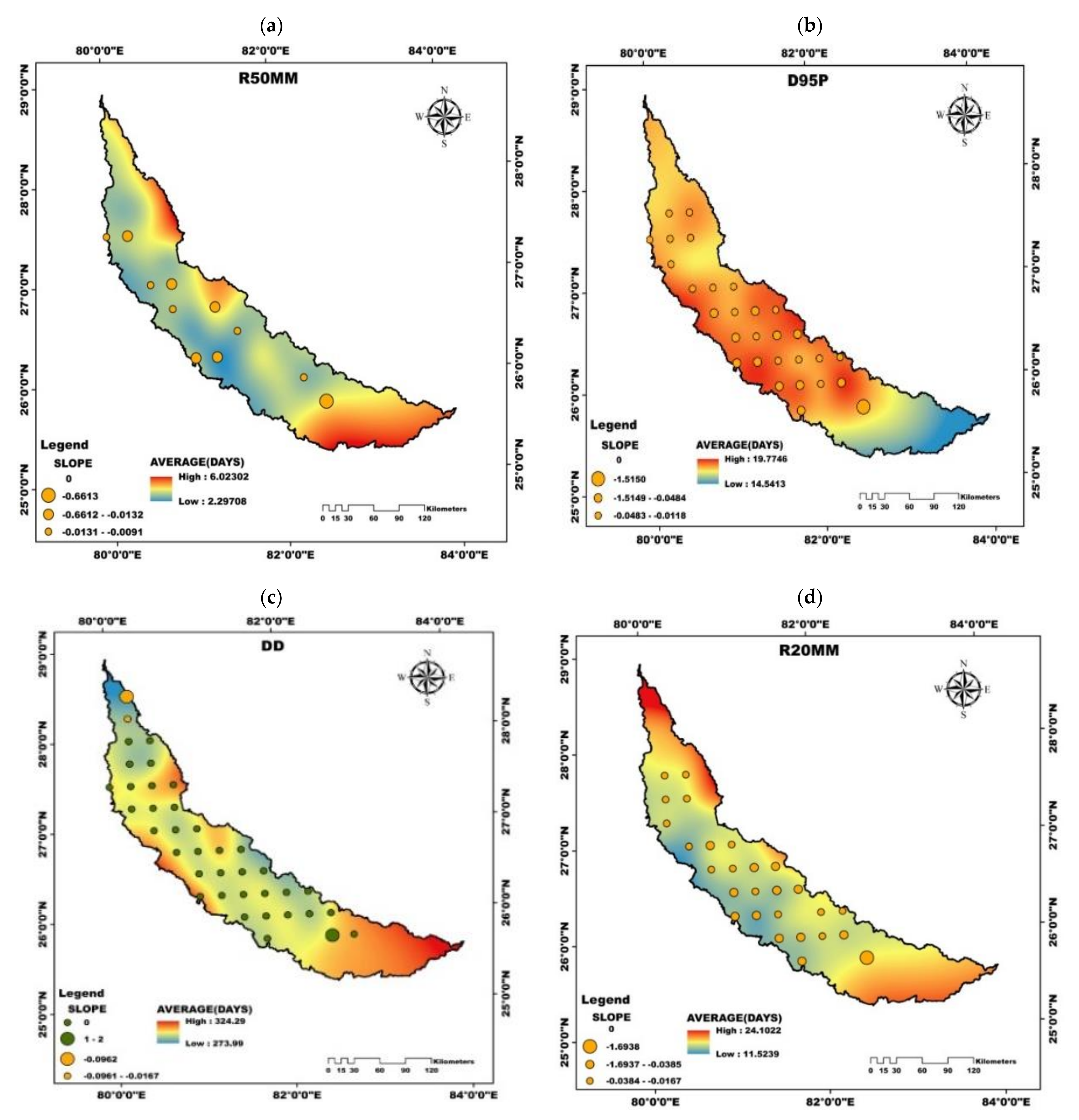
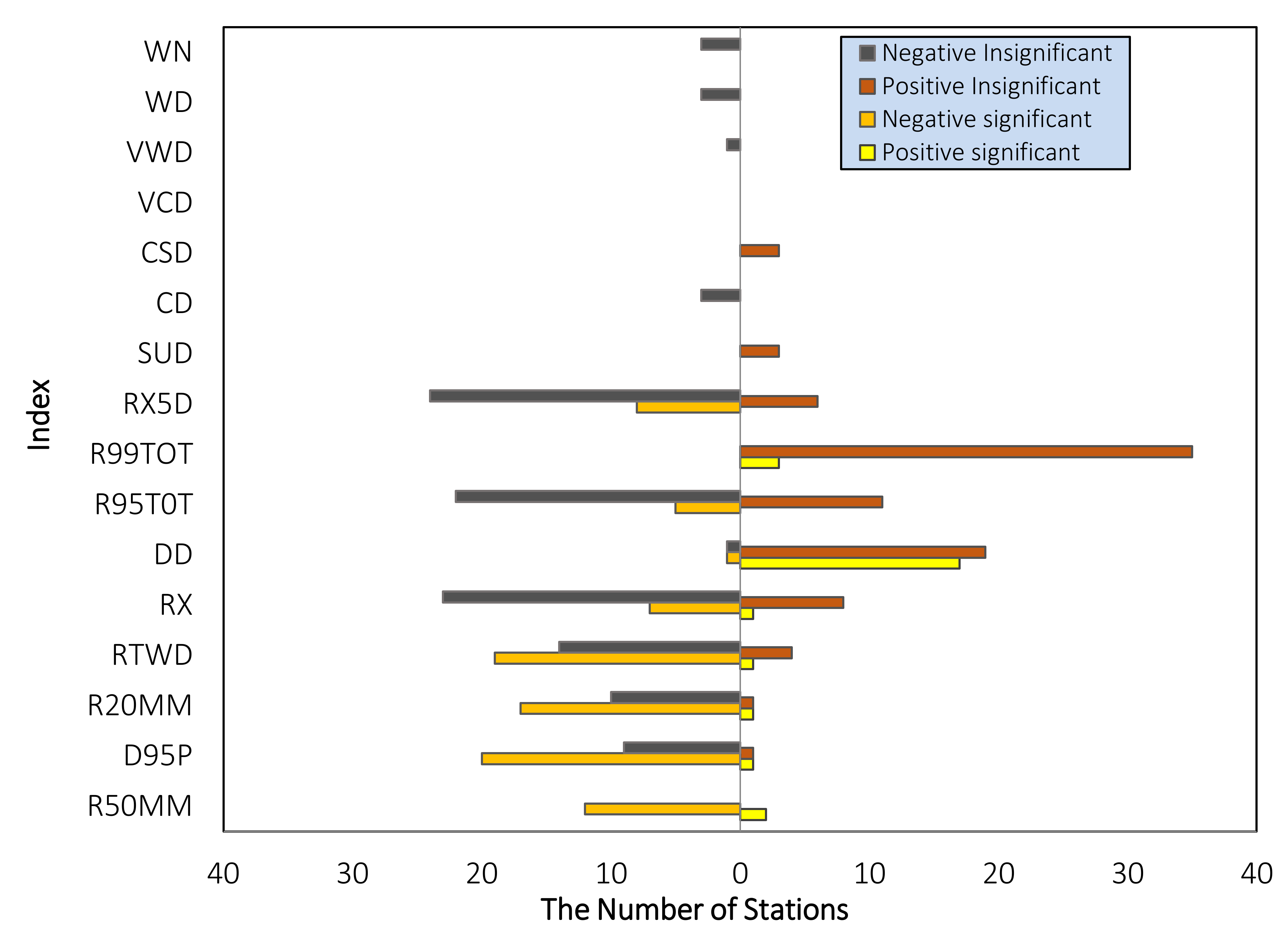
4.2. Spatio-Temporal Variability of Extreme Climate Indices

The spatio-temporal trends in 16 selected extreme climate indices for the entire period is presented in Figure 3. Figure 4 provides a summary of the number of stations showing significant trends of extreme climate indices. The results show a substantial reduction in the precipitation amount over the entire basin, barring few exceptions. This significant negative trend is visible in RTWD, highlighting a considerable decrease during the period with a maximum slope of −3.3002 at the basin’s central region. Although the trends of all the stations are decreasing, 19 stations were statistically significant. R50MM for all stations showed decreasing trends, 12 of which were statistically significant, with higher trend slopes of −0.6613 in the basin’s southern region. D95P showed negative trends for all stations over the basin, out of which 20 were significant and the maximum slope was found to be equal to −1.5150 in the southern region. Further, 17 stations displayed statistically significant negative trends for the index R20MM with maximum slope (−1.6938) being observed at the southern region. A similar pattern of negative trends can be observed with the other precipitation indices such as R95TOT, RX5D, and RX for almost all the stations. The number of dry days (DD) showed positive trends during the period over the basin at 36 stations out of which 17 stations are statistically significant with a maximum slope of 2 at the southern region of the basin. It is evident from the negative trends of various precipitation indices that there is a significant reduction of precipitation over the basin. The index DD exhibiting positive trends over the basin during the same period indicates that the basin has moved towards drier weather.

4.3. Hurst Analysis of Extreme Climate Indices

From the Hurst component the behavior and predictability will be revealed. The nature of the changing pattern can be determined based on the value of the Hurst exponent, with H < 0.5 indicating that the mean is reverting, H = 0.5 indicating that the change is random walk process and H > 0.5 illustrates that the changing pattern is sustainable. Therefore, by knowing the value of H, the intrinsic nature (mean reverting or trending) of the time series can be described and it plays a significant role with implications for forecast skill, low frequency variations [34]. The spatial distribution map of H values for each of the extreme climate indices is presented in Figure 5. The future trends can be determined based on the value of the Hurst exponent obtained for the index. R50MM shows mixed increasing and decreasing future trends all over the basin with the Hurst exponent value around 0.43 and 0.67.

A sustainable decreasing trend is observed for D95P at all stations over the basin, indicating a reduction in precipitation in the future. The number of dry days (DD) exhibits a sustainable decreasing trend at almost all the stations over the basin barring a few exceptions indicating that the basin is turning drier. For R95TOT, a sustainable decreasing trend is displayed at almost all the stations except for five stations that interestingly exhibited the opposite trend of the present pattern. All the stations showed a sustainable decreasing trend for the index RTWD in the basin, indicating that the number of wet days in the basin will reduce in the future. The indices RX, RX5D, and R20MM displayed sustainable decreasing trends over most of the basin stations except for 2–3 stations whose Hurst exponents too are closer to 0.50 indicating that the future trend over the entire basin can be considered as sustainable. Generally, processes with H > 0.5 indicate a persistent long memory effect and the trend is sustainable [16]. Since in the present study, most of the stations show H > 0.5, it shows that this region would be having a persisting phenomenon in terms of decreasing trend in precipitation and increasing trend in temperature in future. After observing the spatial distribution map of extreme climate indices (Figure 5), we can summarize that almost all the extreme precipitation indices exhibit a sustainable decreasing trend except a few stations. Our analysis reveals that precipitation will continue to decrease in the future meaning that the basin is inching towards a drier climate.

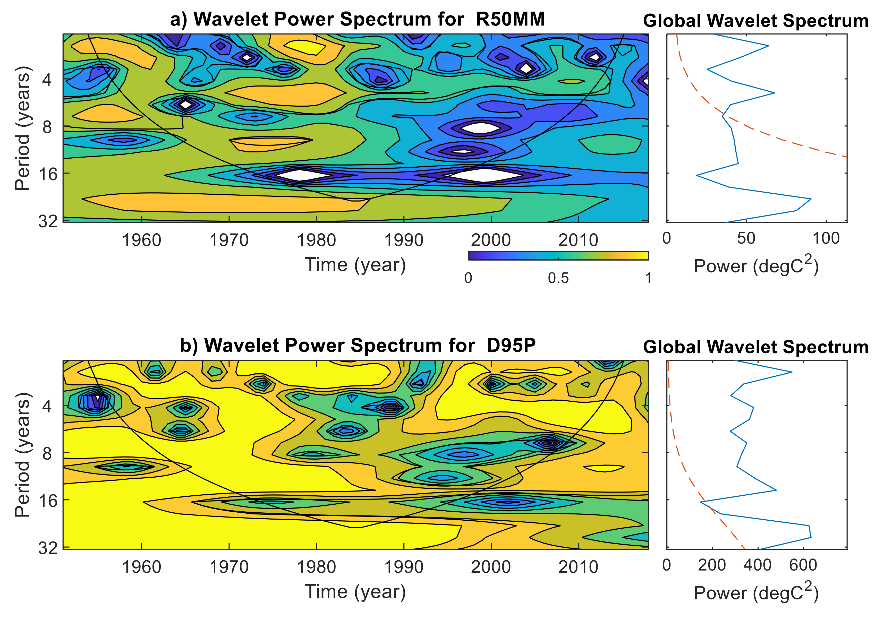
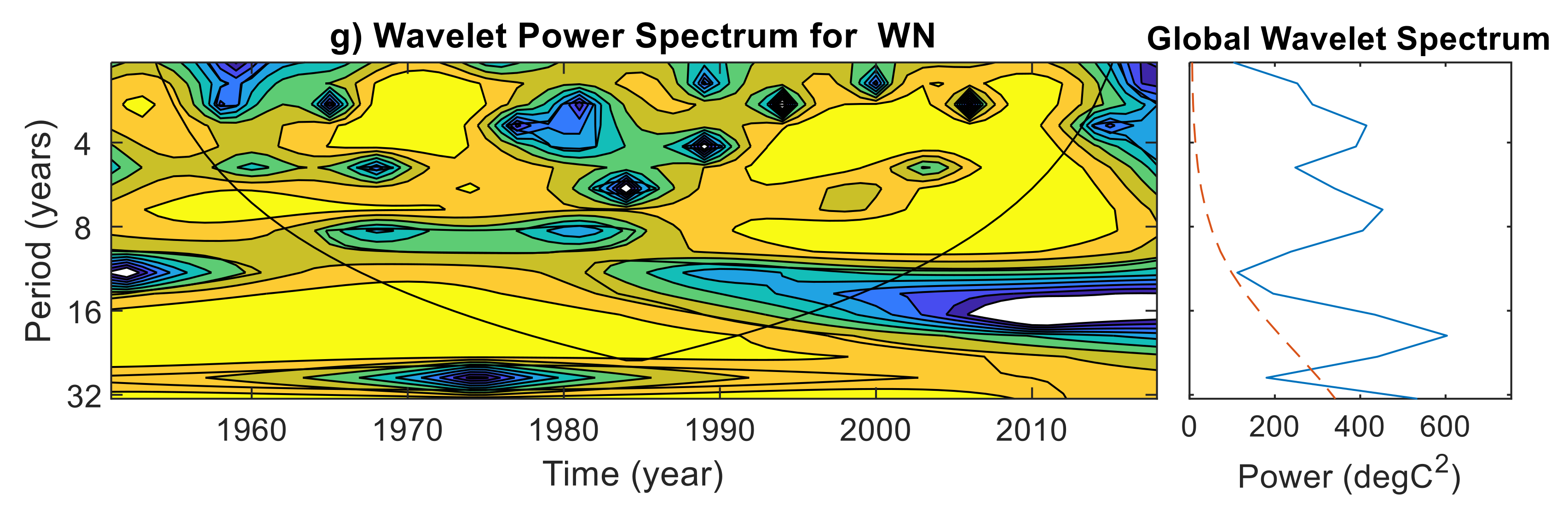
4.4. Periodic Oscillation Analysis

The variability of the climate indices is multifaceted, and often conveyed as multi-frequency and quasi-periodic in the time and frequency domain. Therefore, it is helpful to use wavelet methods for analyzing the variations in the frequency of climate indices at multiple scales averaged over 38 grid points in the Gomati river basin during 1951–2018. In doing so, the regularity of any climate index and its response to climate change can be better understood. Figure 6 shows the wavelet power spectrum for the climate indices, in which contours enclosing light yellow regions have larger power. The cone of influence is represented by a V shape with a black line to distinguish between non-significant periodic characteristics (edge effect artefacts) and significant periodic characteristics (within the cone of influence) at 95% confidence level [42]. Additionally, the global power spectrum and its statistical significance are depicted beside each climate index. The results show that the two-year period was dominant in the global wavelet spectrum of R50MM, with significant wavelet power found during 1975–1980 (Figure 6a). The wavelet power spectrum for D95P showed a significant power distributed across the 2–16-year bands, and the two-year period was dominant in the global power spectrum around 1970–1990 (Figure 6b). One exciting finding unraveled in Figure 6b is that the dominant two-year period of D95P has changed to the four-year after 1984 and remains there in the past two decades. The wavelet power spectrum of R20MM is following a similar pattern of D95P (Figure 6c). Figure 6c indicates that frequency of R20MM is 1 in two years until 1984, and later the frequency has changed to 1 in four years. Figure 6d shows the wavelet power in the 2–4-year band around 1955–1965, 1975–1983, 1990–2002, and 2007–2012 and in the 4–6-year band during 1955–1995, and in the 8–16-year band around 196–2000 of R99TOT. The 8-year period was found in the global wavelet of WD and a 2–4-year band in 1965–1975, 1995–2000 (Figure 6e). The global wavelet power spectrum of CD (Figure 6f) showed that the 4–6-year period was significant at the 95% confidence level during 1970–1980. WN was dominated by four- and eight-year periods, with a 4–8-year band, found in 1994–2014 (Figure 6g).

Overall, the wavelet spectra of most of the extreme climate indices showed variability within the 4–8 years and for some, the inter-decadal variability is prominent. Earlier study by Rathinasamy et al. [50] have shown there is a linkage between extreme precipitation in the Indian subcontinent and the global climate teleconnections such as ENSO and PDO. Following that study, the reason for the presence of dominant variability observed in the extreme climate indices could be linked to global teleconnection patterns. However, in-depth analysis is required to understand the dynamics of this linkage which can be considered in the further analysis.

4.5. Bivariate Joint Probability and Return Period Analysis

The mutual dependence between the hydro-climatic variables helps to understand extreme climate characteristics over time that individual indices are limited to cover [39]. Therefore, to detect and analyze the mutual dependence among the extreme climate in the Gomati river basin bi-variate copula functions are used. Bi-variate copula is efficient to compute the bi-variate joint probabilities and return periods of climate indices. First, the probability distributions of climate indices in the Gomati river basin were calculated using 15 marginal distribution functions (listed in Section 3.4), and then Bayesian Information criterion was used to find the optimal fitting function. The thumb rule is that a smaller BIC value point to better-fitting, with the marginal distribution function to the lowest value considered the best fitted distribution function.

Table 3. BIC values and selection of distribution function of the Expert Team on Climate Change Detection and Indices (ETCCDI).

Climate Index	Type of Distribution Function
	Weibull	Gamma	Birbaum-Saunders	Inverse Gaussian	Log Normal	Nakagami	Log-Logistic	Rayleigh	Normal	Rician
R50MM	241.5	230.6	226.9	226.8	227.0	237.0	228.9	242.8	247.7	243.8
D95P	399.3	393.8	394.0	394.0	394.2	394.5	397.0	446.7	396.6	396.4
R20MM	379.4	373.0	372.8	372.8	373.0	374.2	375.7	416.9	377.1	376.8
RTWD	940.1	928.6	927.2	927.2	927.3	931.0	929.1	985.7	934.8	934.5
RX	628.4	614.7	612.1	612.0	612.2	617.9	615.4	679.0	622.1	621.9
RX5D	725.1	709.2	706.7	706.6	706.6	713.0	706.1	769.1	717.9	717.6
DD	512.3	505.8	505.9	505.9	505.9	505.7	506.7	822.2	505.6	505.6
R95TOT	470.9	462.2	462.0	462.0	462.0	463.7	462.8	514.0	466.6	466.4
R99TOT	410.5	410.1	413.5	414.8	413.9	410.5	416.7	406.3	421.0	410.5
CSD	576.6	581.5	582.3	582.3	582.4	580.8	583.8	811.5	580.1	580.1
WD	371.8	385.9	433.2	437.5	409.7	376.1	385.9	385.7	368.0	368.9
CD	342.9	343.0	347.5	347.7	347.0	341.4	344.3	375.0	341.8	341.6
WN	378.2	383.5	397.5	398.7	393.6	379.2	385.8	387.7	378.6	377.9
SUD	512.6	505.0	505.1	505.1	505.1	505.0	507.7	823.0	505.1	505.0

Italic bold font indicates the selected distribution function.

shows the results of the calculation of BIC values for each distribution for every climate index. Our results show that R50MM, RTWD and RX are inverse Gaussian distributed, D95P is gamma, R20MM is Birnbaum-Saunders, RX5D is log-logistic, DD and WN is Rician, R95TOT is Log-normal, R99TOT is Rayleigh, CSD is Weibull, WD is normal, CD and SUD is Nakagami distributed. As presented in Figure 7, the optimal distribution function revealed above was more effective.

The selected 16 climate indices could be combined into 120 combinations; however, a few combinations lack physical meaning. We attempt two combinations for the Gomati river basin to understand the combination of precipitation amount and intensity (modelling the flood drivers). Firstly, the R95TOT and RTWD combination is selected to calculate the joint probability and return period of extremes contribution to total precipitation and precipitation amount from wet days. Next, the R95TOT and D95P combination is selected to calculate the joint probability and return period of extreme precipitation contribution and number of days. The best copula function was selected based on the minimum principle of AIC and RMSE following [51]. The results are given in

Table 4. Ranking of copula families based on RMSE and AIC values.

Climate Index Combination	Copula Family	RMSE	AIC	Rank
RTWD&R95TOT	Clayton	0.4175	−403.707	3
	Frank	0.2214	−490.013	2
	Gumbell	0.1956	−506.819	1
D95P&R95TOT	Clayton	0.3863	−414.272	3
	Frank	0.2253	−487.603	2
	Gumbell	0.1995	−504.131	1

and the joint probability and return period for two combinations averaged over 53 grid points during 1951–2018 are shown in Figure 8 and Figure 9.

We first calculated the mutual dependence of these climate indices (R95TOT and RTWD) in the 68-year record (68 pairs) using three approaches, i.e., Kendal’s Tau rank (r = 0.4934), Spearman’s rank correlation (r = 0.6613), and Pearson correlation coefficient (r = 0.7428), of which three methods illustrate a statistically significant dependence between R95TOT and RTWD. Hence, the bi-variate copula analysis is applied to describe the interdependence among them.

We first select the optimal marginal distribution functions, to the R95TOT and RTWD based on the BIC goodness-of-fit measure. Figure 7d,h show the fitted distributions (red line) compared to the observed (blue dots) for R95TOT and RTWD. We chose an inverse Gaussian and lognormal distributions to fit both variables (refer to Table 3). Then we evaluated three Archimedean copula families (Clayton, Frank, and Gumbel) using the MvCAT toolbox in MATLAB [51]. The parameters of the copula and their posterior distribution are inferred using a Bayesian analysis and Monte-Carlo simulations. For both combinations, Gumbel is selected as best copula family to describe the dependence structure (see Table 4). Figure 8 shows the isolines of the joint probability (Figure 8c) and return period (Figure 8f) based on the Gumbel copula. We then use the Gumbel copula model to derive non-exceedance probabilities and return periods and analyze the compound event. For the most likely design scenario, the values of R95TOT and RTWD are 48% and 1500 mm, respectively. The joint return period’s resulting values are greater than values resulting from univariate analysis (R95TOT with 44% and RTWD of 1450 mm). The difference in values highlights that ignoring the mutual dependence can lead to a substantial underestimation of extremes. Similarly, for another combination (R95TOT and D95P), the same procedure is followed to derive the joint return periods and displayed in Figure 9. Intuitively, consideration of mutual dependence improves the accuracy of the return period of climate extremes.

Overall, from the entire analysis, spatio-temporal variability and changing pattern of extreme climate indices indicate that the basin will experience a reduction in precipitation and an increase in the number of dry days pushing the basin towards drier weather. This finding is in line with prior studies dealt globally [17,52,53] as well as regionally [54,55,56,57,58]. In particular, Abeysingha et al. [56], after analyzing rainfall and temperature trends in the Gomati River basin, concluded that there had been a significant reduction in rainfall, consequently leading to decline in the streamflow coupled with increasing temperature results in dryness in the basin. Sachidanand et al. [58] concluded that the number of ‘warm days’ per year increased significantly, whereas the number of ‘cold days’, ‘warm nights’, and ‘cold nights’ per year decreased significantly at several locations in India. On the other side, a decreasing trend in precipitation is observed at some Uttar Pradesh locations, including the Gomati basin, highlighting the possibility of dryness in Northern India.

Numerous climate models have observed that there has been an increase in surface temperatures over the 20th century [52]. This increase in temperatures will lead to increased evaporation and surface drying, which increases the intensity and duration of drought events. On the other hand, for every 1 °C warming, the moisture-holding capacity of air is increased by about 7%, thereby leading to an increase in water vapor in the atmosphere, which in turn leads to intensifying the water cycle [59]. Therefore, a warmer climate will increase the risk of drought due to surface dryness and floods due to intensified water cycle but at different times and/or places. A similar pattern is observed in the present study. There has been a significant reduction in precipitation along with an increase in the number of dry days. The future trends based on the Hurst exponent indicate that this trend is likely to continue in the near future. Further copula modelling is applied to analyze compound extremes. Intuitively, the multivariate framework can better represent the risk due to the consideration of mutual dependence.

5. Conclusions

We investigated the long-term spatiotemporal variation of precipitation and the extreme climate indices in the Gomati River Basin in India. The extreme climate indices were characterized through a trend analysis, dominant periodicities and joint probability. The main conclusions from the study are as follows.

(a)

Different extreme precipitation indices (D95P, R95TOT) show significant decreasing trends whereas the extreme temperature indices show an increasing trend indicating that the basin is experiencing a warm and dry climate compared to the past. Further, the positive persistence present in these variables show that the trend would continue in the future resulting in warmer and drier climate. The results presented in the study is in congruence with the other studies wherein the climate has become warmer

(b)

The presence of the significant periodicities (4–8 years and decadal timescale) in the precipitation extreme indicate a possibility of connection with some of the well-known global atmospheric patterns such as ENSO and PDO. However, interestingly, the extreme temperature indices did not exhibit significant periodicities.

(c)

Further, the analysis from the CWT of the extreme precipitation indices indicate that there is a significant non-stationarity indicating that the changes in the precipitation patterns after the 1980s.

(d)

Further copula modelling is applied to analyze compound extremes. The multivariate framework better represented the risk due to the consideration of mutual dependence. Interestingly, the copula modelling shows that the joint probabilities for higher annual precipitation and precipitation receiving from very wet days are smaller than the marginal exceedance probabilities. Intuitively, consideration of mutual dependence improves the compound risk of climate extremes.

References

1. Stocker, T.F.; Qin, D.; Plattner, G.-K.; Alexander, L.V.; Allen, S.K.; Bindoff, N.L.; Bréon, F.-M.; Church, J.A.; Cubasch, U.; Emori, S.; et al. Technical summary. In Climate Change 2013: The Physical Science Basis. Contribution of Working Group I to the Fifth Assessment Report of the Intergovernmental Panel on Climate Change; Cambridge University Press: Cambridge, UK, 2013; pp. 33–115. [Google Scholar]
2. Mutiibwa, D.; Vavrus, S.J.; McAfee, S.A.; Albright, T.P. Recent Spatiotemporal Patterns in Temperature Extremes across Conterminous United States. J. Geophys. Res. Atmos. 2015, 120, 7378–7392. [Google Scholar] [CrossRef]
3. Shrestha, U.B.; Shrestha, B.B. Climate Change Amplifies Plant Invasion Hotspots in Nepal. Divers. Distrib. 2019, 25, 1599–1612. [Google Scholar] [CrossRef] [Green Version]
4. Van Wilgen, B.W.; Fill, J.M.; Baard, J.; Cheney, C.; Forsyth, A.T.; Kraaij, T. Historical Costs and Projected Future Scenarios for the Management of Invasive Alien Plants in Protected Areas in the Cape Floristic Region. Biol. Conserv. 2016, 200, 168–177. [Google Scholar] [CrossRef]
5. Zhou, Y.; Ren, G. Change in Extreme Temperature Event Frequency over Mainland China, 1961–2008. Clim. Res. 2011, 50, 125–139. [Google Scholar] [CrossRef] [Green Version]
6. Shukla, R.; Chakraborty, A.; Sachdeva, K.; Joshi, P.K. Agriculture in the Western Himalayas—An Asset Turning into a Liability. Dev. Pract. 2018, 28, 318–324. [Google Scholar] [CrossRef]
7. El-Zein, A.; Tonmoy, F.N. Assessment of Vulnerability to Climate Change Using a Multi-Criteria Outranking Approach with Application to Heat Stress in Sydney. Ecol. Indic. 2015, 48, 207–217. [Google Scholar] [CrossRef] [Green Version]
8. Bahinipati, C.S.; Venkatachalam, L. Role of Climate Risks and Socio-Economic Factors in Influencing the Impact of Climatic Extremes: A Normalisation Study in the Context of Odisha, India. Reg. Environ. Chang. 2016, 16, 177–188. [Google Scholar] [CrossRef]
9. Shukla, R.; Agarwal, A.; Sachdeva, K.; Kurths, J.; Joshi, P.K. Climate Change Perception: An Analysis of Climate Change and Risk Perceptions among Farmer Types of Indian Western Himalayas. Clim. Chang. 2019, 152, 103–119. [Google Scholar] [CrossRef]
10. Zhang, J.; Terrones, M.; Park, C.R.; Mukherjee, R.; Monthioux, M.; Koratkar, N.; Kim, Y.S.; Hurt, R.; Frackowiak, E.; Enoki, T.; et al. Carbon Science in 2016: Status, Challenges and Perspectives. Carbon 2016, 98, 708–732. [Google Scholar] [CrossRef]
11. Stocker, T.F.; Clarke, G.K.C.; Le Treut, H.; Lindzen, R.S.; Meleshko, V.P.; Mugara, R.K.; Palmer, T.N.; Pierrehumbert, R.T.; Sellers, P.J.; Trenberth, K.E.; et al. Physical Climate Processes and Feedbacks. In IPCC, 2001: Climate Change 2001: The Scientific Basis. Contribution of Working Group I to the Third Assessment Report of the Intergovernmental Panel on Climate Change; Houghton, J.T., Ding, Y., Griggs, D.J., Noguer, M., van der Linden, P.J., Dai, X., Maske, K., Eds.; Cambridge University Press: Cambridge, UK, 2001; pp. 417–470. ISBN 978-0-521-01495-3. [Google Scholar]
12. Easterling, D.R. Climate Extremes: Observations, Modeling, and Impacts. Science 2000, 289, 2068–2074. [Google Scholar] [CrossRef] [Green Version]
13. Farajzadeh, H.; Matzarakis, A. Quantification of Climate for Tourism in the Northwest of Iran: Quantification of climate for tourism in the northwest of iran. Meteorol. Appl. 2009, 16, 545–555. [Google Scholar] [CrossRef]
14. Keggenhoff, I.; Elizbarashvili, M.; Amiri-Farahani, A.; King, L. Trends in Daily Temperature and Precipitation Extremes over Georgia, 1971–2010. Weather Clim. Extrem. 2014, 4, 75–85. [Google Scholar] [CrossRef] [Green Version]
15. Ruml, M.; Gregorić, E.; Vujadinović, M.; Radovanović, S.; Matović, G.; Vuković, A.; Počuča, V.; Stojičić, D. Observed Changes of Temperature Extremes in Serbia over the Period 1961–2010. Atmos. Res. 2017, 183, 26–41. [Google Scholar] [CrossRef]
16. Guo, E.; Zhang, J.; Wang, Y.; Quan, L.; Zhang, R.; Zhang, F.; Zhou, M. Spatiotemporal Variations of Extreme Climate Events in Northeast China during 1960–2014. Ecol. Indic. 2019, 96, 669–683. [Google Scholar] [CrossRef]
17. Zhang, X.; Alexander, L.; Hegerl, G.C.; Jones, P.; Tank, A.K.; Peterson, T.C.; Trewin, B.; Zwiers, F.W. Indices for Monitoring Changes in Extremes Based on Daily Temperature and Precipitation Data: Indices for Monitoring Changes in Extremes. WIREs Clim. Chang. 2011, 2, 851–870. [Google Scholar] [CrossRef]
18. García-Cueto, O.R.; Cavazos, M.T.; de Grau, P.; Santillán-Soto, N. Analysis and Modeling of Extreme Temperatures in Several Cities in Northwestern Mexico under Climate Change Conditions. Theor. Appl. Climatol. 2014, 116, 211–225. [Google Scholar] [CrossRef]
19. Wang, H.; Zhang, G.; Li, N.; Zhang, B.; Yang, H. Soil Erodibility as Impacted by Vegetation Restoration Strategies on the Loess Plateau of China: Effect of Vegetation Restoration on Soil Erodibility. Earth Surf. Process. Landf. 2019, 44, 796–807. [Google Scholar] [CrossRef]
20. Sharma, P.J.; Loliyana, V.D.; Resmi, S.R.; Timbadiya, P.V.; Patel, P.L. Spatiotemporal Trends in Extreme Rainfall and Temperature Indices over Upper Tapi Basin, India. Theor. Appl. Climatol. 2018, 134, 1329–1354. [Google Scholar] [CrossRef]
21. Abeysingha, N.; Singh, M.; Sehgal, V.; Khanna, M.; Pathak, H. Analysis of Rainfall and Temperature Trends in Gomti River Basin. J. Agric. Phys. 2014, 14, 56–66. [Google Scholar]
22. Dutta, V.; Kumar, R.; Sharma, U. Assessment of Human-Induced Impacts on Hydrological Regime of Gomti River Basin, India. Manag. Environ. Qual. Int. J. 2015, 26, 631–649. [Google Scholar] [CrossRef]
23. Pai, D.; Sridhar, L.; Rajeevan, M.; Sreejith, O.; Satbhai, N.; Mukhopadhyay, B. Development of a New High Spatial Resolution (0.25 × 0.25) Long Period (1901–2010) Daily Gridded Rainfall Data Set over India and Its Comparison with Existing Data Sets over the Region. Mausam 2014, 65, 1–18. [Google Scholar]
24. Srivastava, A.K.; Rajeevan, M.; Kshirsagar, S.R. Development of a High Resolution Daily Gridded Temperature Data Set (1969–2005) for the Indian Region. Atmos. Sci. Lett. 2009, 10, 249–254. [Google Scholar] [CrossRef]
25. Guntu, R.K.; Maheswaran, R.; Agarwal, A.; Singh, V.P. Accounting for Temporal Variability for Improved Precipitation Regionalization Based on Self-Organizing Map Coupled with Information Theory. J. Hydrol. 2020, 590, 125236. [Google Scholar] [CrossRef]
26. Guntu, R.K.; Rathinasamy, M.; Agarwal, A.; Sivakumar, B. Spatiotemporal Variability of Indian Rainfall Using Multiscale Entropy. J. Hydrol. 2020, 587, 124916. [Google Scholar] [CrossRef]
27. Pingale, S.M.; Khare, D.; Jat, M.K.; Adamowski, J. Spatial and Temporal Trends of Mean and Extreme Rainfall and Temperature for the 33 Urban Centers of the Arid and Semi-Arid State of Rajasthan, India. Atmos. Res. 2014, 138, 73–90. [Google Scholar] [CrossRef]
28. Alexander, L.V.; Fowler, H.J.; Bador, M.; Behrangi, A.; Donat, M.G.; Dunn, R.; Funk, C.; Goldie, J.; Lewis, E.; Rogé, M.; et al. On the Use of Indices to Study Extreme Precipitation on Sub-Daily and Daily Timescales. Environ. Res. Lett. 2019, 14, 125008. [Google Scholar] [CrossRef]
29. Sen, P.K. Robustness of Some Nonparametric Procedures in Linear Models. Ann. Math. Stat. 1968, 39, 1913–1922. [Google Scholar] [CrossRef]
30. Lettenmaier, D.P.; Wood, E.F.; Wallis, J.R. Hydro-Climatological Trends in the Continental United States, 1948–1988. J. Clim. 1994, 7, 586–607. [Google Scholar] [CrossRef] [Green Version]
31. Yue, S.; Hashino, M. Long term trends of annual and monthly precipitation in japan1. JAWRA J. Am. Water Resour. Assoc. 2003, 39, 587–596. [Google Scholar] [CrossRef]
32. Partal, T.; Kahya, E. Trend Analysis in Turkish Precipitation Data. Hydrol. Process. 2006, 20, 2011–2026. [Google Scholar] [CrossRef]
33. Koutsoyiannis, D. Hydrologic Persistence and the Hurst Phenomenon. In Water Encyclopedia; Lehr, J.H., Keeley, J., Eds.; John Wiley & Sons, Inc.: Hoboken, NJ, USA, 2005; p. sw434. ISBN 978-0-471-47844-7. [Google Scholar]
34. Graves, T.; Gramacy, R.; Watkins, N.; Franzke, C. A Brief History of Long Memory: Hurst, Mandelbrot and the Road to ARFIMA, 1951–1980. Entropy 2017, 19, 437. [Google Scholar] [CrossRef] [Green Version]
35. Maheswaran, R.; Khosa, R. Comparative Study of Different Wavelets for Hydrologic Forecasting. Comput. Geosci. 2012, 46, 284–295. [Google Scholar] [CrossRef]
36. Agarwal, A.; Maheswaran, R.; Kurths, J.; Khosa, R. Wavelet Spectrum and Self-Organizing Maps-Based Approach for Hydrologic Regionalization—A Case Study in the Western United States. Water Resour. Manag. 2016, 30, 4399–4413. [Google Scholar] [CrossRef]
37. Tamaddun, K.A.; Kalra, A.; Ahmad, S. Wavelet Analyses of Western US Streamflow with ENSO and PDO. J. Water Clim. Chang. 2017, 8, 26–39. [Google Scholar] [CrossRef] [Green Version]
38. Nicolay, S.; Mabille, G.; Fettweis, X.; Erpicum, M. 30 and 43 Months Period Cycles Found in Air Temperature Time Series Using the Morlet Wavelet Method. Clim. Dyn. 2009, 33, 1117–1129. [Google Scholar] [CrossRef]
39. Narasimha, R.; Bhattacharyya, S. A Wavelet Cross-Spectral Analysis of Solar–ENSO–Rainfall Connections in the Indian Monsoons. Appl. Comput. Harmon. Anal. 2010, 28, 285–295. [Google Scholar] [CrossRef] [Green Version]
40. Farge, M. Wavelet Transforms and Their Applications to Turbulence. Annu. Rev. Fluid Mech. 1992, 24, 395–458. [Google Scholar] [CrossRef]
41. Torrence, C.; Compo, G.P. A Practical Guide to Wavelet Analysis. Bull. Am. Meteorol. Soc. 1998, 79, 61–78. [Google Scholar] [CrossRef] [Green Version]
42. Yeditha, P.K.; Venkatesh, K.; Maheswaran, R.; Ankit, A. Forecasting of extreme flood events using different satellite precipitation products and wavelet-based machine learning methods. Chaos Interdiscip. J. Nonlinear Sci. 2020, 30, 063115. [Google Scholar]
43. Sklar, M. Fonctions de Repartition an Dimensions et Leurs Marges. Publ. Inst. Statist. Univ. Paris 1959, 8, 229–231. [Google Scholar]
44. Ganguli, P.; Merz, B. Extreme Coastal Water Levels Exacerbate Fluvial Flood Hazards in Northwestern Europe. Sci. Rep. 2019, 9, 1–14. [Google Scholar] [CrossRef]
45. Anandalekshmi, A.; Panicker, S.T.; Adarsh, S.; Muhammed Siddik, A.; Aloysius, S.; Mehjabin, M. Modeling the Concurrent Impact of Extreme Rainfall and Reservoir Storage on Kerala Floods 2018: A Copula Approach. Model. Earth Syst. Environ. 2019, 5, 1283–1296. [Google Scholar] [CrossRef]
46. Nelsen, R.B. An Introduction to Copulas; Springer Science & Business Media: Berlin/Heidelberg, Germany, 2007. [Google Scholar]
47. Genest, C.; Rivest, L.-P. Statistical Inference Procedures for Bivariate Archimedean Copulas. J. Am. Stat. Assoc. 1993, 88, 1034–1043. [Google Scholar] [CrossRef]
48. Ghosh, S.; Vittal, H.; Sharma, T.; Karmakar, S.; Kasiviswanathan, K.S.; Dhanesh, Y.; Sudheer, K.P.; Gunthe, S.S. Indian Summer Monsoon Rainfall: Implications of Contrasting Trends in the Spatial Variability of Means and Extremes. PLoS ONE 2016, 11, e0158670. [Google Scholar] [CrossRef]
49. Singh, D.; Ghosh, S.; Roxy, M.K.; McDermid, S. Indian Summer Monsoon: Extreme Events, Historical Changes, and Role of Anthropogenic Forcings. WIREs Clim. Chang. 2019, 10. [Google Scholar] [CrossRef]
50. Rathinasamy, M.; Agarwal, A.; Sivakumar, B.; Marwan, N.; Kurths, J. Wavelet Analysis of Precipitation Extremes over India and Teleconnections to Climate Indices. Stoch. Environ. Res. Risk Assess. 2019, 33, 2053–2069. [Google Scholar] [CrossRef]
51. Sadegh, M.; Ragno, E.; AghaKouchak, A. Multivariate C Opula A Nalysis T Oolbox (MvCAT): Describing Dependence and Underlying Uncertainty Using a B Ayesian Framework. Water Resour. Res. 2017, 53, 5166–5183. [Google Scholar] [CrossRef]
52. Solomon, S. IPCC (2007): Climate Change the Physical Science Basis. In Proceedings of the Agu Fall Meeting Abstracts, San Francisco, CA, USA, 10–14 December 2007; Volume 2007, p. U43D-01. [Google Scholar]
53. Alexander, L.V.; Zhang, X.; Peterson, T.C.; Caesar, J.; Gleason, B.; Klein Tank, A.M.G.; Haylock, M.; Collins, D.; Trewin, B.; Rahimzadeh, F.; et al. Global Observed Changes in Daily Climate Extremes of Temperature and Precipitation. J. Geophys. Res. 2006, 111, D05109. [Google Scholar] [CrossRef] [Green Version]
54. Arora, M.; Goel, N.K.; Singh, P. Evaluation of Temperature Trends over India/Evaluation de Tendances de Température En Inde. Hydrol. Sci. J. 2005, 50, 12. [Google Scholar] [CrossRef]
55. Kothawale, D.; Munot, A.; Krishna Kumar, K. Surface Air Temperature Variability over India during 1901–2007, and Its Association with ENSO. Clim. Res. 2010, 42, 89–104. [Google Scholar] [CrossRef]
56. Guntu, R.K.; Agarwal, A. Investigation of Precipitation Variability and Extremes Using Information Theory. Environ. Sci. Proc. 2021, 4, 14. [Google Scholar] [CrossRef]
57. Kurths, J.; Agarwal, A.; Marwan, N.; Rathinasamy, M.; Caesar, L.; Krishnan, R.; Merz, B. Unraveling the spatial diversity of Indian precipitation teleconnections via nonlinear multi-scale approach. Nonlinear Process. Geophys. 2019, 26, 251–266. [Google Scholar] [CrossRef] [Green Version]
58. Kumar, S.; Chanda, K.; Pasupuleti, S. Spatiotemporal Analysis of Extreme Indices Derived from Daily Precipitation and Temperature for Climate Change Detection over India. Theor. Appl. Climatol. 2020, 140, 343–357. [Google Scholar] [CrossRef]
59. Trenberth, K. Changes in Precipitation with Climate Change. Clim. Res. 2011, 47, 123–138. [Google Scholar] [CrossRef] [Green Version]
Figure 1. Indian map showing the Uttar Pradesh state and the Gomati river basin boundary in the green and orange color, respectively. Dots in the Gomati river basin show selected precipitation grid points.
Atmosphere 12 00480 g001
Figure 2. Spatio Temporal trends in the total precipitation at different time scales, (ad) monthly, (e) seasonal, and (f) annual. The figure provides the Sen slope of the trend in each grid, which has significant trends.
Atmosphere 12 00480 g002aAtmosphere 12 00480 g002b
Figure 3. Grid locations having significant trends in the selected extreme climate indices expressed along with the trend line’s slope for (a) R50MM, (b) D95P, (c) DD, (d) R20MM, (e) R95TOT, (f) RX5D, (g) RTWD, and (h) RX.
Atmosphere 12 00480 g003aAtmosphere 12 00480 g003b
Figure 4. Number of stations where extreme climate indices have shown specific trends in the Gomati river basin during 1901–2018.
Atmosphere 12 00480 g004
Figure 5. Spatial distribution map of extreme climate indices (a) R50MM, (b) D95P, (c) DD, (d) R95TOT, (e) RTWD, (f) R20MM, (g) RX, and (h) RX5D in Gomati Basin based on the Hurst Exponent.
Atmosphere 12 00480 g005aAtmosphere 12 00480 g005b
Figure 6. Continuous wavelet transformation for climate indices (a) R50MM, (b) D95P, (c) R20MM, (d) R95TOT, (e) WD, (f) CD, and (g) WN averaged over 38 grid points in the Gomati river basin during 1951–2018. The V shape represents the cone of influence and regions enclosed with light yellow are periods with significant power. The red color dashed line distinguishes between significant and non-significant periods. If the global wavelet spectrum curve is higher than the dashed line at a particular scale, then the period is statistically significant at the 95% confidence level.
Atmosphere 12 00480 g006aAtmosphere 12 00480 g006bAtmosphere 12 00480 g006c
Figure 7. Observed data (blue dots) and fitted marginal distribution (red line) of the climate indices (a) R50MM, (b) D95P, (c) R20MM, (d) RTWD, (e) RX, (f) RX5D, (g) DD, (h) R95TOT, (i) R99TOT, (j) CSD, (k) WD, (l) CD, (m) WN, and (n) SUD averaged over 36 grid points in the Gomati river basin during 1951–2018.
Atmosphere 12 00480 g007aAtmosphere 12 00480 g007bAtmosphere 12 00480 g007c
Figure 8. Cumulative distributive functions of (A) R95TOT and (B) RTWD, and their (D) and (E) are associated univariate periods (y-axis indicated in log scale). Joint probability iso lines derived from the Gumbell copula are displayed in Figure (C), and the associated return period isolines are illustrated in Figure (F). The colorbar [0 1] represents the joint density levels of joint probability and return periods, where 0 represents lower and one represents higher density level. Blue dots represent the observed pairs of R95TOT and RTWD. The figure is plotted using the MvCAT toolbox [51] in MATLAB (Version 9.4 R 2020b).
Atmosphere 12 00480 g008
Figure 9. Same as Figure 8 but for a combination of climate indices R95TOT and D95P.
Atmosphere 12 00480 g009