
An Observational Study of Aerosols and Tropical Cyclones over the Eastern Atlantic Ocean Basin for Recent Hurricane Seasons


1
Center for Applied Atmospheric Research and Education, San Jose State University, San Jose, CA 95192, USA
2
NOAA Cooperative Science Center in Atmospheric Sciences and Meteorology, Howard University, Washington, DC 20001, USA
*
Author to whom correspondence should be addressed.
Atmosphere 2021, 12(8), 1036; https://0-doi-org.brum.beds.ac.uk/10.3390/atmos12081036
Submission received: 28 June 2021
/
Revised: 28 July 2021
/
Accepted: 6 August 2021
/
Published: 13 August 2021
(This article belongs to the Special Issue Tropical Cyclone Evolution: Changes in Structure, Intensity, and Environmental Interactions)
Abstract
:The aerosol vertical distribution in the tropical cyclone (TC) main development region (MDR) during the recent active hurricane seasons (2015–2018) was investigated using observations from NASA’s Cloud-Aerosol Lidar and Infrared Pathfinder Satellite Observations (CALIPSO) Satellite. The Total Attenuated Backscatter (TAB) at 532 nm was measured by the Cloud-Aerosol Lidar with Orthogonal Polarization (CALIOP Lidar) onboard CALIPSO which is a polar orbiting satellite that evaluates the role clouds and atmospheric aerosols play in Earth’s weather, climate and air quality. The TAB was used to illustrate the dispersion and magnitude of the aerosol vertical distribution in the TC-genesis region. A combination of extinction quality flag, cloud fraction, and cloud-aerosol discrimination (CAD) scores were used to filter out the impact of clouds. To better describe the qualitative and quantitative difference of aerosol along the paths of African Easterly Waves (AEWs), the MDR was further divided into two domains from 18° W to 30° W (Domain 1) and 30° W to 45° W (Domain 2), respectively. The distribution of average aerosol concentration from the time of active cyclogenesis was compared and quantified between each case. The resulting observations suggest that there are two distinct layers of aerosols in the vertical profile, a near surface layer from 0.5–1.75 km and an upper layer at 1.75–5 km in altitude. A quantification of the total aerosol concentration values indicate domain 2 cases were associated with higher aerosol concentrations than domain 1 cases. The environmental variables such as sea surface temperature (SST), vertical windshear (VWS), and relative humidity (RH) tended to be favorable for genesis to occur. Among all cases in this study, the results suggested tropical cyclone genesis and further development occurred under dust-loaded conditions while the environmental variables were favorable, indicating that dust aerosols may not play a significant role in inhibiting the genesis process of TCs.
1. Introduction
It is imperative to improve our observational understanding of tropical cyclone (TC) activities and to further develop accurate TC forecasting models. Specifically, in the Atlantic Ocean basin, as African Easterly Waves (AEW) propagate westward off the coast of West Africa, they begin to decrease in sea level pressure if the environmental conditions are favorable (e.g., mesoscale convective systems) thus forming a closed surface circulation leading to TC genesis (e.g., Gray 1968; Tompkins and Chiao 2011) [1,2]. Schade (2000) [3] found higher sea surface temperature (SST) to be directly associated with the intensification of TCs. Karloski and Evans (2016) [4] suggested the seasonal variation of the duration of the TC season is primarily controlled by interannual variability in the conditions necessary for TC formation. Similarly, Kossin (2008) [5] found that a consistent pattern of warmer SSTs extended the period of the Atlantic hurricane season. Therefore, the environmental factors that influence the development of TCs can also influence the duration of an individual storm and the length of the season. Furthermore, the upper-level atmosphere can provide supplementary support for the development of a TC due to an upper-level trough being present in the path of the tropical wave (Montgomery and Farrell 1993) [6]. Moreover, in synoptic conditions, mid to upper-level wind speeds tend to be stronger than the surface causing unfavorable shearing to occur on convection that is assembling for TCs (Demaria 1996) [7]. An environmental influence that does not sustain the development of a TC, such as vertical wind-shear, can prevent the TC from developing further (Holland 1997) [8].
In addition to warm sea surface temperatures (SSTs) amongst unstable atmospheric conditions conducive for TC activities, there is a strong relationship among Saharan Air Layer (SAL), vertical distribution of dust aerosols and atmospheric convection influence (Propsero 2013) [9]. Dust loading is often associated with very dry air which acts as a factor for TC development. Nevertheless, how exactly dust aerosols influence tropical cyclones are observationally elusive. The increased dust loading and transport occurring into the eastern Atlantic Ocean basin strongly implicated the stronger winds associated with AEWs as a major influence on TC variability (Jones et al., 2003) [10]. Lau and Kim (2007) [11] found evidence that high dust loading scenarios were inversely proportional to SST. This indicates that the SAL could be indirectly influencing TC genesis through essential elements such as SST. Sun et al. (2008) [12] conducted a comparative analysis between the 2005 and 2007 Atlantic hurricane seasons to understand cyclone activity in terms of how many TCs were produced. They found that 2007 was relatively less active than the 2005 hurricane season, possibly a function of enhanced dust loading from SAL in 2007. Additionally, 2005 had much higher SST and moisture content compared to 2007. Jenkins et al. (2008) [13] investigated the linkages between Saharan dust and TC rain band. They suggested that while the SAL can create hostile thermodynamics and kinematic environmental conditions for TC genesis, it also provides an infusion of cloud condensation nuclei (CCN) and ice nuclei (IN) which potentially invigorate convection. Moreover, continental aerosol dust outbreaks influence the increase of stratocumulus clouds in the Atlantic Ocean basin which could apply additional heating during the genesis process (Amiri-Farahani et al., 2017) [14].
Bretl et al. (2015) [15] further explained the complexity behind the influence of dust on the development of TCs due to the warming of SAL; however, no significant change in the frequency was discovered. Dunion and Velden (2004) [16] suggested SAL negatively influences TC activity through dry air intrusion, mid-easterly jet inducing localized wind shear, and the enhancement of the preexisting trade wind inversion which can stabilize the environment. Model analysis by Gorgan et al. (2016) [17] showed that dust radiative effects furthered the growth of AEW by the likelihood of dust allowing an AEW to maintain itself as the zonally varying flow is dampened. Zhang et al. (2009) [18] conducted a study in which aerosols were entrained into the eyewall structure of the TC. They found that when CCN was added into the atmosphere there was a direct increase in cloud droplet number concentration but a decrease in droplet size [18]. However, aerosols can change physical and thermodynamic processes in TCs through droplet growth and latent heat exchange (Zhang et al., 2009) [18].
Braun (2010) [19] suggested that SAL could be overemphasized by prior research as a negative influence towards genesis rather than a positive. It is a common assumption that Saharan dust outbreaks are strongly associated with dry air, which could easily hinder the development of TCs. However, Braun (2010) [19] found that there was not much evidence that supported Saharan dust negatively influencing TC genesis; instead, SAL could be adding energy to AEWs due to it being a source for the African Easterly Jet (AEJ). More specifically, the AEJ can influence background cyclonic vorticity, supporting TC genesis [19]. Saharan dust also can be scavenged and redistributed through the atmosphere by TCs and AEWs (Sauter and L’Ecuyer 2017) [20]. This redistribution of dust caused by an AEW can influence the location at which aerosols are possibly entrained into other developing TCs [20].
Dry air entrainment at the surface can inhibit tropical cyclone development as vertical transport reduces the moist environment needed for sustainable convection (Fritz and Wang 2013) [21]. The location at which aerosols are entrained into TCs could be an important element in regard to how the genesis process is affected. Braun et al. (2013) [22] used NASA’s CALIPSO satellite to locate dust layers during TC Helene’s propagation westward in the Atlantic Ocean basin. They found minimal dust in the dry air layer and saw a large dust layer propagate westward ahead of the storm. While many studies provide insight into possible interactions between dust and TC genesis, the lack of quantitative analysis of aerosols during the development stage of TCs raises uncertainties. Moreover, observations are essential to the evaluation of these models that incorporate factors such as dust loading and entrainment processes.
In this study, data from NASA’s CALIPSO satellite was used to investigate the influence of Saharan dust during TC formation. The quality filters developed by Tackett et al. (2018) [23] for CALIPSO satellite data have been updated in this study to accurately account for aerosol type and concentration in the vertical atmosphere. In this paper, the locations at which TC genesis and further development occurred and the extent to which aerosols had an influence using a dust threshold value was evaluated.
In this study, the extent to which dust aerosols had an influence during the genesis stage and beyond was evaluated using the CALIPSO LIDAR-derived 532 nm backscatter concentration values. Other viable factors including SST, VWS, and RH were also evaluated with the associated TC genesis case under a dust outbreak condition. Section 2 provides case descriptions and methods behind the research associated with data processing. The results on each TC are presented in Section 3. A summary of the key findings and future work are discussed in Section 4.
2. Cases and Data Processing
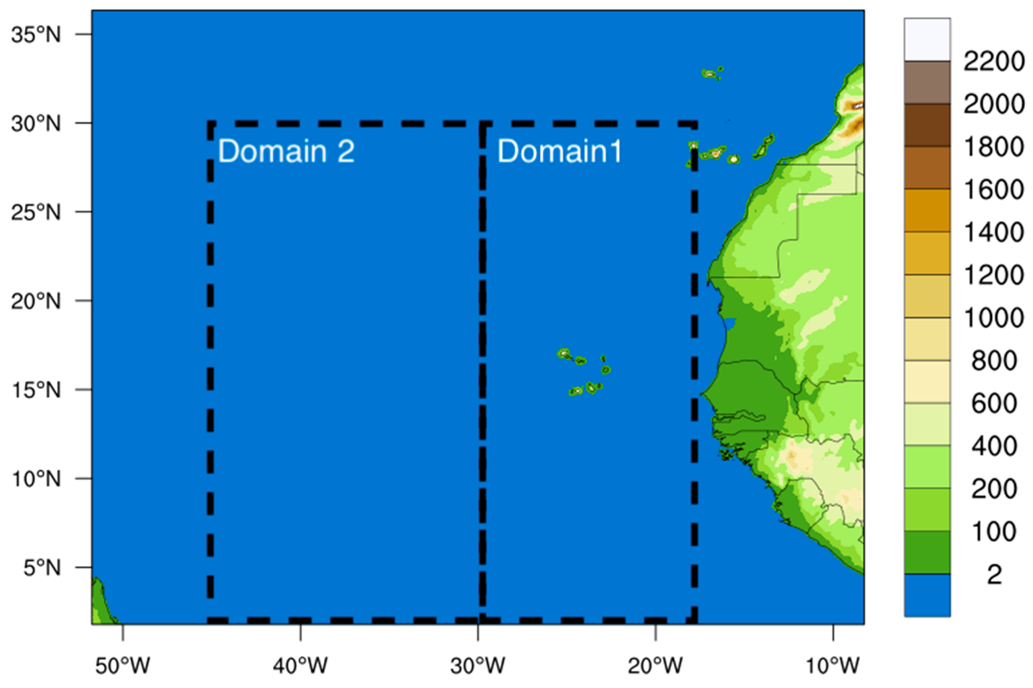
Tropical cyclones were selected with genesis processes through dust outbreaks during 2015–2018, including Florence (2018), Irma (2017), Fiona (2016), Gaston (2016), Lisa (2016), Matthew (2016), Danny (2015), and Grace (2015). The study region was divided into two domains to classify the TC formation location. As shown in Figure 1, domain 1 was defined between 18° W to 30° W while domain 2 was bounded between 45° W to 30° W. Splitting the region into two domains helps determine not only the propagation of the tropical cyclone concerning the dust outbreak but also the extent of other factors (i.e., SST, and wind shear) that play into the genesis of TCs. Generally, domain 1 presents relatively lower SST, wind-shear, and RH. In comparison, domain 2, which encompasses a large part of the main development region for TCs, reveals more favorable conditions for development. All TC cases went through genesis in domains 1 and 2 except for Matthew (2016) which developed outside of domain 2.
Satellite data from the NASA Terra/MODIS were used to examine spatial variability in dust outbreak events. NASA’s Cloud-Aerosol Lidar with Orthogonal Polarization (CALIOP) onboard the CALIPSO Satellite was employed to evaluate vertical profiles of atmospheric aerosols. Figure 2 shows the eight TCs and the overpass location of CALIPSO. The Total Attenuated Backscatter (TAB) at wavelength 532 nm measured by CALIOP Lidar was the main parameter analyzed [24]. TAB is defined as the signal received by the satellite that measures the backscatter of the lidar signal by molecules and particles in the atmosphere (Kar et al., 2018) [25]. In this study, TAB is used to illustrate the vertical distribution and magnitude of the aerosol concentration around the TC-genesis region. Filters such as the Cloud-Aerosol Distribution Score (CAD Score), Cloud Layer Fraction (CLF), and 532 nm Quality Flag (QC) are applied to reduce cloud interference and other contaminating features in the vertical profile. The CAD Score uses a confidence function to discriminate between clouds and aerosols based on their optical and physical properties (Liu et al., 2009) [26]. CAD > 90% was selected to omit the cloud interference on aerosol signatures. The CLF is used to obtain a cloud clearing fractional distribution of backscatter in each bin for aerosol backscatter. In each 5 km profile bin there are 30 single shot cloud layers. To omit ambiguous aerosol data that would misclassify an aerosol layer as a cloud layer, the CLF was set to reject anything greater than 28 for each bin. The 532 nm Quality Flag Extinction (QFE) is another layer of filtering that can assess the aerosols for quality analysis. Young and Vaughan (2018) [27] suggest that night retrievals are higher quality than daytime retrievals; therefore, a constraint of QC = 16 is implemented to identify the totally attenuating and opaque features. This additional constraint refines the data quality and cloud/noise interference. In this study, TAB restraints from 1.0 × 10⁻³ km−1sr−1 through 1.0 × 10⁻² km−1sr−1 are chosen to depict an aerosol threshold. The QC flag and CLF cleans the concentration levels where we see higher signatures that could be false, and the CAD score used in the algorithm eliminates contaminated features that have a 90% confidence level of being clouds.
In this study, the first 200–500 m were omitted to avoid sea spray contamination near the surface. Furthermore, the anomaly of the specific CALIPSO pass during genesis was then developed based on a monthly 4 year (2015–2018) average (e.g., August and September). This information exemplifies whether the aerosol concentration associated with the TC during the time of genesis was above or below the monthly 4 year average.
The European Centre for Medium-Range Weather Forecasts (ECMWF) ERA-Interim data (i.e., 0.75 degree spatial resolution) are used to develop surface analysis, wind shear, and relative humidity (RH) temporal analyses [28,29]. The surface analyses designate areas focused on a possible genesis location. Vertical wind shear (VWS) of 250 hPa and 850 hPa were used to access the wind field aloft. Furthermore, the 700 hPa RH was used to illustrate the moisture environment during the time of genesis and to assess if any dry air layer was involved. Finally, sea surface temperature data (SST) was obtained from the NOAA OI SST V2 high-resolution dataset to incorporate a two-day average before genesis occurred [30]. Ocean Heat Suite (SOHS) from the National Environmental Satellite Data and Information Service (NESDIS) was used to obtain the depth of the 26 °C isothermal layer and the ocean heat content [31]. Monthly anomalies of SST are calculated to evaluate the TC development conditions. With the combination of SST, MSLP, VWS, and RH, a comparative case analysis was constructed to evaluate to what extent aerosols played a role in developing a TC during its genesis stage. With the coherent overlap of the CALIPSO Satellite observation and reanalysis, an assessment will be carried out to understand the extent to which aerosols had a positive or negative correlation with the development of TCs during the time of genesis.
3. Results
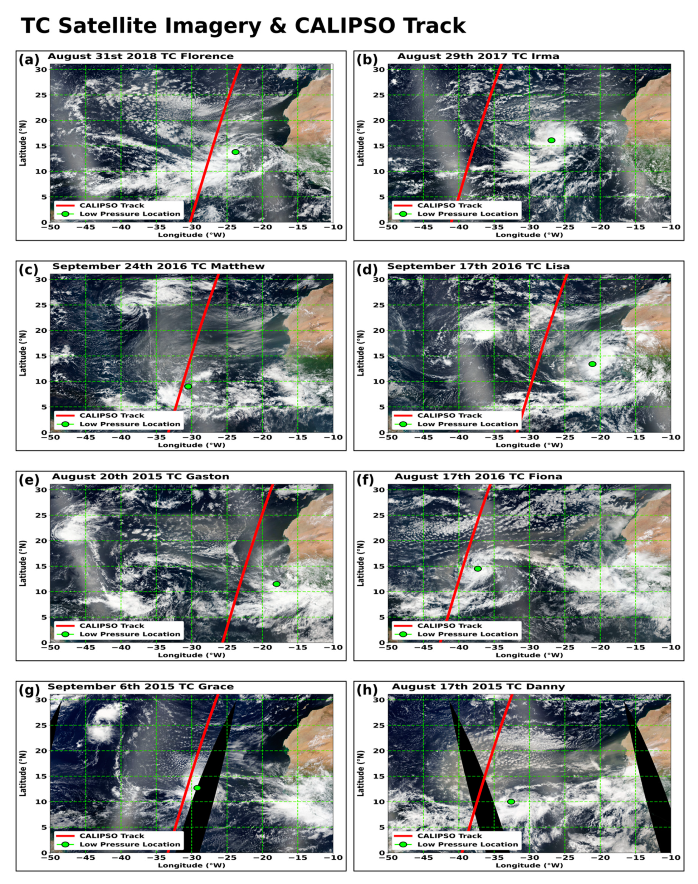
The perspective events are each shown with TERRA/MODIS visual satellite imagery with its selected CALIPSO pass in order to assess the vertical profile (Figure 2). Table 1 shows each case’s CALIPSO satellite pass date, genesis date, and domain location. As a result, five cases went through genesis in domain 1 and two cases went through genesis in domain 2. Furthermore, the majority of cases had CALIPSO pass a day before genesis took place, while others were a day or two after the pass. The importance of evaluating the dust aerosol concentration ahead of the developing TC before genesis takes place exemplifies the interaction that is bound to occur as the TC moves into the air mass. By evaluating the spatial variability of the satellite pass and the location of the AEW, a proper observational analysis of TAB can be assessed.
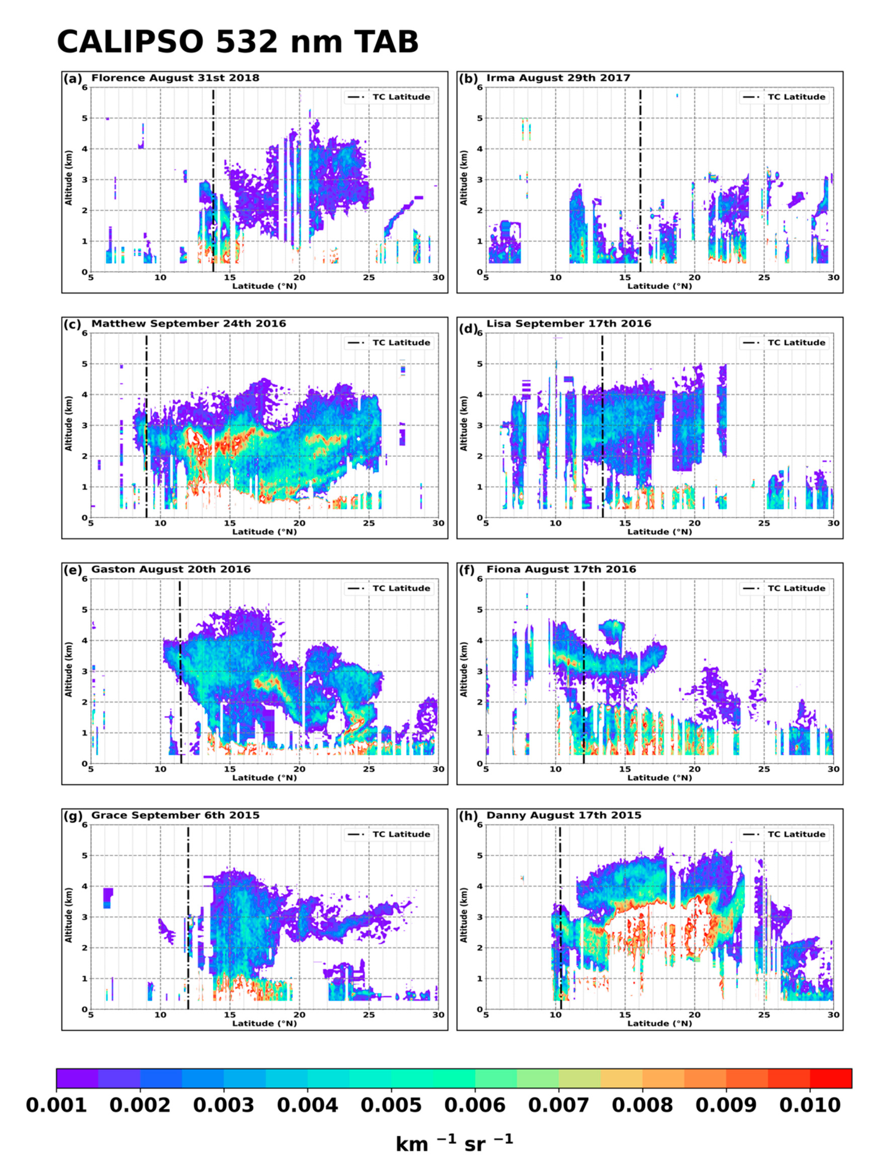
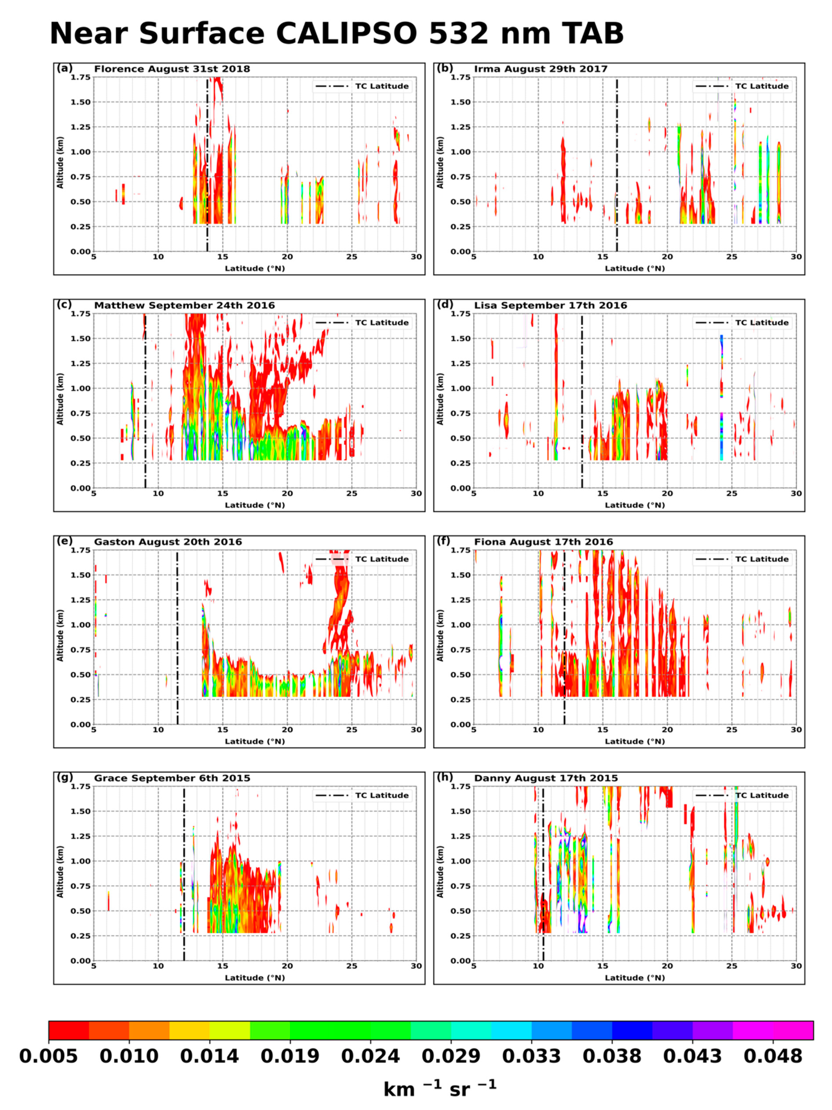
In-situ observations of TAB were examined during dust outbreak events and at the time of developing TCs. As shown in Figure 3, much of the aerosol backscatter detected for each case was occurring between the near-surface level to 5 km. It can be further broken up into two layers (i.e., above/below 1.75 km above sea level) for a specific depiction of where the aerosol backscatter is found in the vertical profile (Figure 3). The first layer can be defined around 2.5 to 5 km above sea level which consists of mostly dust aerosols that usually covers a large latitudinal area between 10° N–20° N (Figure 3). The second layer that can be seen is from the 0.25–1.75 km above sea level (Figure 4). The second layer is primarily where a dense mixture of dust and marine aerosols can be found. Therefore, spatial and concentration variability was analyzed to determine the extent of the direct relationship.
3.1. Dust Concentration Variability
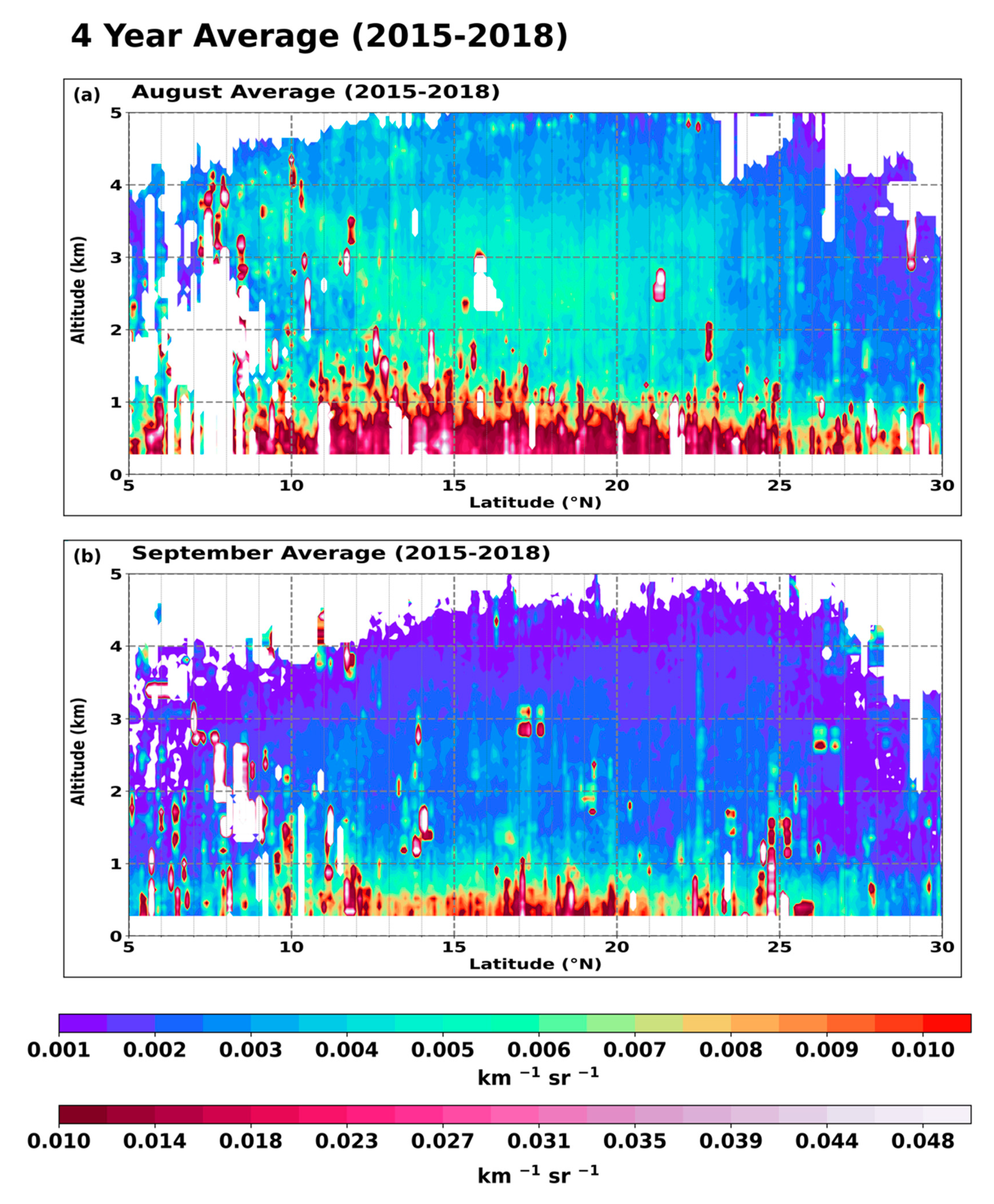
The dust concentration variability amongst cases gives further insight into the relationship of developing TCs in association with the total amount of aerosols and where they are located vertically. Figure 5 shows the 4 year (2015–2018) climatology of TAB for August and September. It can be seen that a robust aerosol concentration occurred near the surface in August. It appears that higher aerosol concentrations are observed during the ramping up of the Atlantic Hurricane season in August. Subsequently, the direct aerosol association during the TC formation stage can be seen from the TAB anomaly of each individual case and the 4 year climatology results (Figure 6).
As shown in Figure 6a,b, the weakest observed aerosol concentration cases were Florence (2018) and Irma (2017). Nevertheless, it is important to note both Irma (2017) and Florence (2018) continued to intensify after genesis had occurred as indicated by the NHC official report [32]. The observed TAB for Florence near the genesis latitude was near 0.004–0.006 km−1sr−1 at 1.5–3 km above sea level (Figure 3a), while the concentration increased to approximately 0.01–0.011 km−1sr−1 near the surface (Figure 4a). Visually seen on the satellite imagery in Figure 2a, CALIPSO made a pass approximately 2–3 degrees away from the center location of Florence. This proximity reveals a decent observational representation of the TAB concentration interacting with the developing TC. Nevertheless, not all cases had such great spatial representation for the satellite observations. Overall, within the boundary of 15°–20° N, TAB was observed at 0.001–0.004 km−1sr−1 from 1–4 km above sea level for all cases (Figure 3). These results show that aerosols are not only in layers but also in clumped areas, as is characteristic of the dust plume. For Irma (2017), a thicker dust layer near the TC is distinguished compared to the satellite pass location, which was further away (Figure 2b). For this CALIPSO pass, the observed concentration was approximately 0.001–0.004 km−1sr−1 from 1–2.5 km above sea level (Figure 3b). The majority of these observations were seen at the near-surface level, where, in some regions, TAB exceeded 0.006 km−1sr−1 (e.g., Figure 4b). The higher values at the near surface are a possible representation of denser dust aerosol particulates in that given region. However, the TAB concentration, as shown in Figure 3b, could have been higher than what was observed if the CALIPSO passed closer to the system.
After analyzing multiple cases, some similarities are evident in the following ways. First, each case’s observed CALIPSO swath was through a dust layer ahead of the AEW (e.g., Figure 2a–g). This observation suggests the dust plume and a TC interaction would be eminent within 24–48 h. Consequently, the dust layers are either already impacting the development of a TC or will with the system within 48 h. TAB concentrations for Lisa (2016), Gaston (2016), Fiona (2016), and Grace (2015) showed a distinct upper aerosol layer from the 2–4 km range averaging between 0.005 and 0.007 km−1sr−1 (Figure 3d–g). The pattern remains consistent as aerosols can also be seen rising in altitude as they approach the TC formation latitude (e.g., dash line in Figure 3e-g). It is suspected that aerosols are essential in the lower to mid part of the troposphere for CCN increase in the development process of a TC. Additionally, near-surface TAB shows excessive concentration levels amongst these cases from 0.01 to 0.02 km−1sr−1 (Figure 4d–g). In general, a very high concentration mimics that of clouds but can also be depicted as very strong scattering feedbacks coming from large dust particles. (Liu et al. 2009) [26].
Danny (2015), which underwent genesis in domain 2, observed a strong TAB signature. (Figure 1). The maximum observed TAB for Danny was approximately 0.0125 km−1sr−1 from the 2.5–5 km altitude range (Figure 3h). A thick layer of dust can also be seen on the MODIS satellite imagery covering a vast area ahead and above the TC (Figure 2h). Moreover, there is a positive anomaly associated with Danny indicating the TC was involved with above average aerosols compared to the 4 year August average (Figure 5a and Figure 6h). Despite being in a high dust concentration area, Danny went through genesis and developed into a hurricane within 48 h.
Matthew (2016) had a very different outcome in the genesis process due to the lack of organization in domain 1 and 2. On 24 September 2016, Matthew (2016) formed in association with a strong dust outbreak event (Figure 2c). Similar to Danny, Matthew also observed a positive anomaly of TAB (Figure 6c). A noteworthy feature for Matthew was that a distinct upper-aerosol layer (2 to 3 km above sea level) concentration of 0.004–0.009 km−1sr−1 (Figure 3c). Furthermore, the near-surface (0.25 to 1 km above sea level) aerosol layer was also averaging between 0.02–0.025 km−1sr−1 and can be seen rising in altitude (Figure 4c).
Figure 7 summarizes the total accumulation of TAB from 10° to 20° N that represents the swath of the CALIPSO satellite overpass. The accumulated TAB within the swath demonstrates Lisa, Gaston, Fiona, and Grace, with a concentration between 16–19 km−1sr−1. A noteworthy feature such as dust aerosols intruding into the center circulation of TC Fiona provided visual evidence of aerosol interaction while genesis was taking place. (e.g., Figure 2d).
The accumulated TAB for both Danny and Matthew had the highest total of TAB concentration amongst all the cases between 30–40 km−1sr−1 (Figure 7). One major difference between Matthew and Danny is the location of the highest aerosol concentration. As seen from Figure 6c,h, Danny observed a maximum positive anomaly primary between 2–3.5 km above sea level while, Matthew observed a maximum positive anomaly at both 0.5–1 km and 2–3 km above sea level. This result may explain why the genesis did not take place in domain 1. However, other environmental factors could have limited the process of genesis to occur rather than the dust aerosols themselves.
To further assess the magnitude of impact dust aerosols may have on tropical development a comparison between cases with dust and a case with minimal to no dust can be evaluated. Evidently, on 31 August 2017, a tropical wave emerged into the eastern Atlantic Ocean basin approximately between 9°–10° N and was associated with little to no dust aerosols as seen on NASA Worldview Terra/MODIS imagery. The NHC classified the tropical wave as a low at 06 UTC on September 4th with genesis taking place in 24 hrs at 06 UTC September 5th and it was classified as tropical storm Jose at 12 UTC [33]. Additionally, the development process took place under an environment with a lack of highly concentrated dust aerosols. As seen from the CALIPSO 532 nm TAB within a 3 degree distance from the convection activity observed dust concentration between 0.0015–0.0020 km−1sr−1 [34]. Compared to the rest of the cases in this study, this observational result of Jose was determined to be one of the smallest amongst the group. The favorable environment of high SSTs and low vertical windshear supports the genesis and development of the system to take place in such a short amount of time.
3.2. Vertical Windshear Analysis
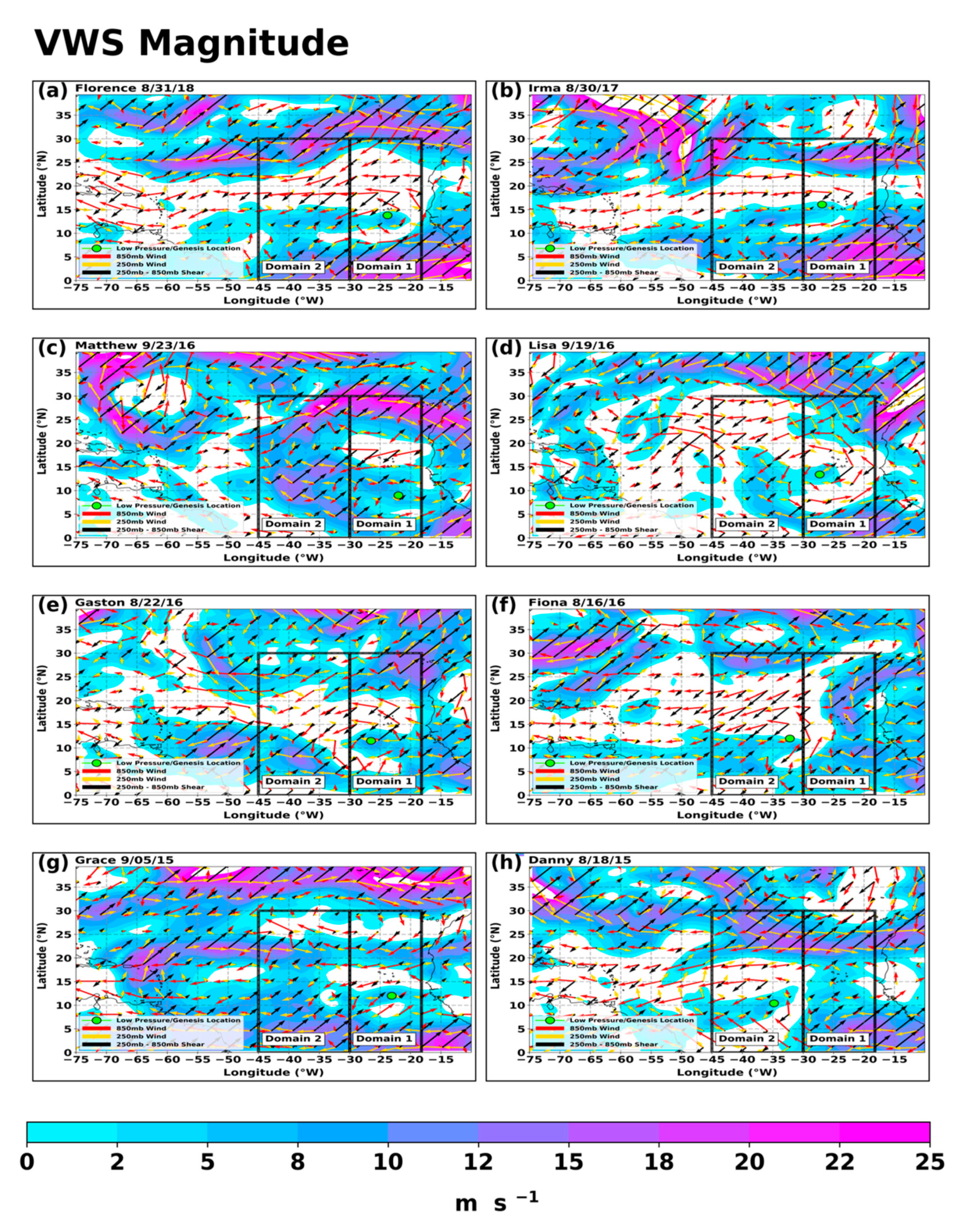
Assessment of the magnitude of vertical wind shear (VWS) of 250–850 hPa is shown in Figure 8. It was found that the VWS was moderately weak for all cases in the given location of genesis. Generally, all cases moved west or northwest due to the trade winds in the MDR and synoptic scale steering flows. Given a radius of 3 degrees from the center of the genesis location, stronger VWS did exit for some cases. However, the shear did not act as a negative influence due to a cyclonic circulation aloft behaving consistently with the flow at the near-surface level. For example, as shown in Figure 8a, Florence had a distinct 850 hPa cyclonic flow (red arrows) which weakened when approaching the 250 hPa level (yellow arrows). There was some shear present between the 250–850 hPa level (black arrows). This scenario is common in most cases, and it is likely due to the similar synoptic-scale conditions during the North Atlantic Hurricane season.
Additionally, the wind shear environment revealed a reoccurring condition which existed within newly formed TCs. For example, Fiona (2016) went through genesis under favorable conditions but started to make its way towards a more shear prone environment within 24 h (Figure 8f). Matthew (2016) was also in a favorable area on the 23rd of September; however, the flow near the surface (red arrows) was weak, preventing the wave from consolidating and going through genesis (Figure 8c). Moving forward in time, the directional shear environment within the 250–850 hPa increases, and conditions become unfavorable as the system propagates through domain 2. Grace (2015) has a belt of windshear from 8~15 ms−1 engulfing the 20° N–25° N region for both domain 1 and 2 (Figure 8g). This shear flow pattern likely kept Grace from advecting northward during the genesis process while an area of dry air was present in that region. Additionally, Gaston (2016) revealed that the storm induced shear of approximately 10 ms−1 was likely due to the broader circulation becoming more organized towards its center amongst a gyre of convergence (Figure 8e). Moreover, Florence and Irma had a very similar magnitude of shear associated with the system with the addition of a belt of shear lying ahead in domain 2 for about 5~12 ms−1 (Figure 8a,b). An interesting feature to note is the wavelike crest feature seen ahead of the location of genesis, indicating a favorable environment for intensification (Figure 8a,b).
3.3. Relative Humidity Analysis
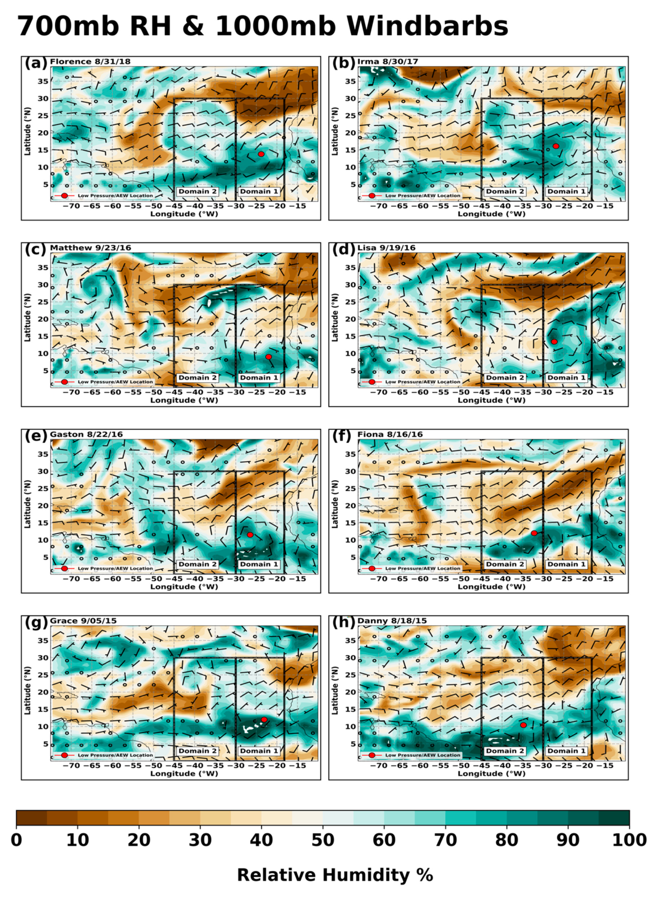
The relative humidity (RH) at the 700 hPa level was critical to the analysis due to its representation of the SAL location in the domain regions. Figure 9 displays 700 hPa RH overlayed with the 1000 hPa winds. All events showed prominent signs of an easterly and northeasterly dry airflow in domain 1 (Figure 9). The results suggest that drier air is being engulfed from the African continent into the domain’s development region. Additionally, dry air, in most cases, is also associated with dust aerosols embedded within the SAL. This inference can be made with the combination of factors shown in Figure 3, Figure 9 and Figure 10. Florence and Irma were broad circulating AEW’s with moisture consolidating in all quadrants of the system during genesis (Figure 9a,b). Lisa, Gaston, and Fiona show the dry air intruding into the system’s west and southwest quadrants (Figure 9d–f). Most of the cases had a favorable environment for development with a relative humidity at 700 hPa between 70 and 90%.
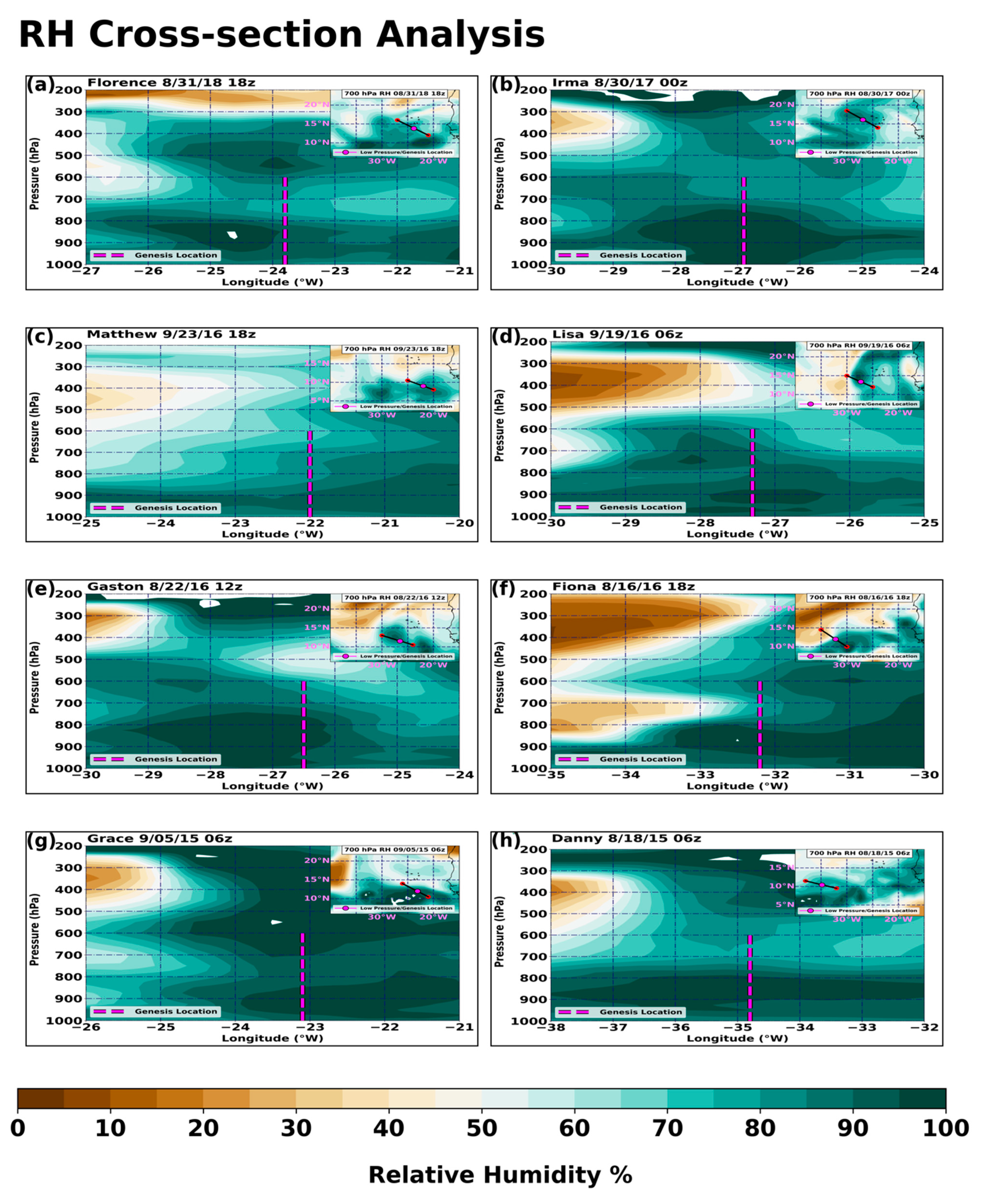
The cross-section analyses for RH illustrate a spatial representation in the horizontal and vertical direction of the atmosphere (Figure 10). For Matthew, Lisa, Fiona, and Grace the dry air intrusion is approximately 1 degree from the center’s location (Figure 10c,d,f,g). Furthermore, Florence, Irma, and Danny see some extent of SAL coming into play by a difference of only 2 degrees longitude (Figure 10a,b,h). Additionally, Fiona (2016) had the highest contrast of dryness as RH dropped to 35% with less than a degree distance from the genesis location (Figure 10f). Moreover, there were signs of a distinct layer of moisture at the 900 hPa level at the center of the genesis location with drier air intruding aloft at 700 hPa (Figure 10f).
An anomalous case such as Irma (2017) was engulfed in a thick moisture bubble from 1000 hPa to 700 hPa where RH exceeded 95% (Figure 10b). This vertical depth was greater than what was observed from Matthew, Lisa, Gaston, and Danny, which immediately started to see a drop in RH well before reaching 700 hPa (Figure 10c–e,h). An interesting feature in the cross-sectional analysis was the dry air presence behind the cases during genesis. For Florence, Irma Lisa, Gaston, and Danny, dry air was already wrapping behind the system’s 700 hPa above sea level (Figure 10a,b,d,e,h). Nearly all cases had drier air ahead of the genesis location at the 700 hPa level during the time of genesis. Despite hostile conditions aloft and displaced by 1–2 degrees of longitude from the TC genesis location, genesis still occurred in a moderate to high RH percentage between the 1000 hPa to 700 hPa vertical atmosphere level for all cases. In addition to VWS and RH, evaluating the SST and OHC is also an important factor in the genesis of TCs.
3.4. Ocean Heat Content (OHC) and Isothermal Layer Depth (ISO) Analysis
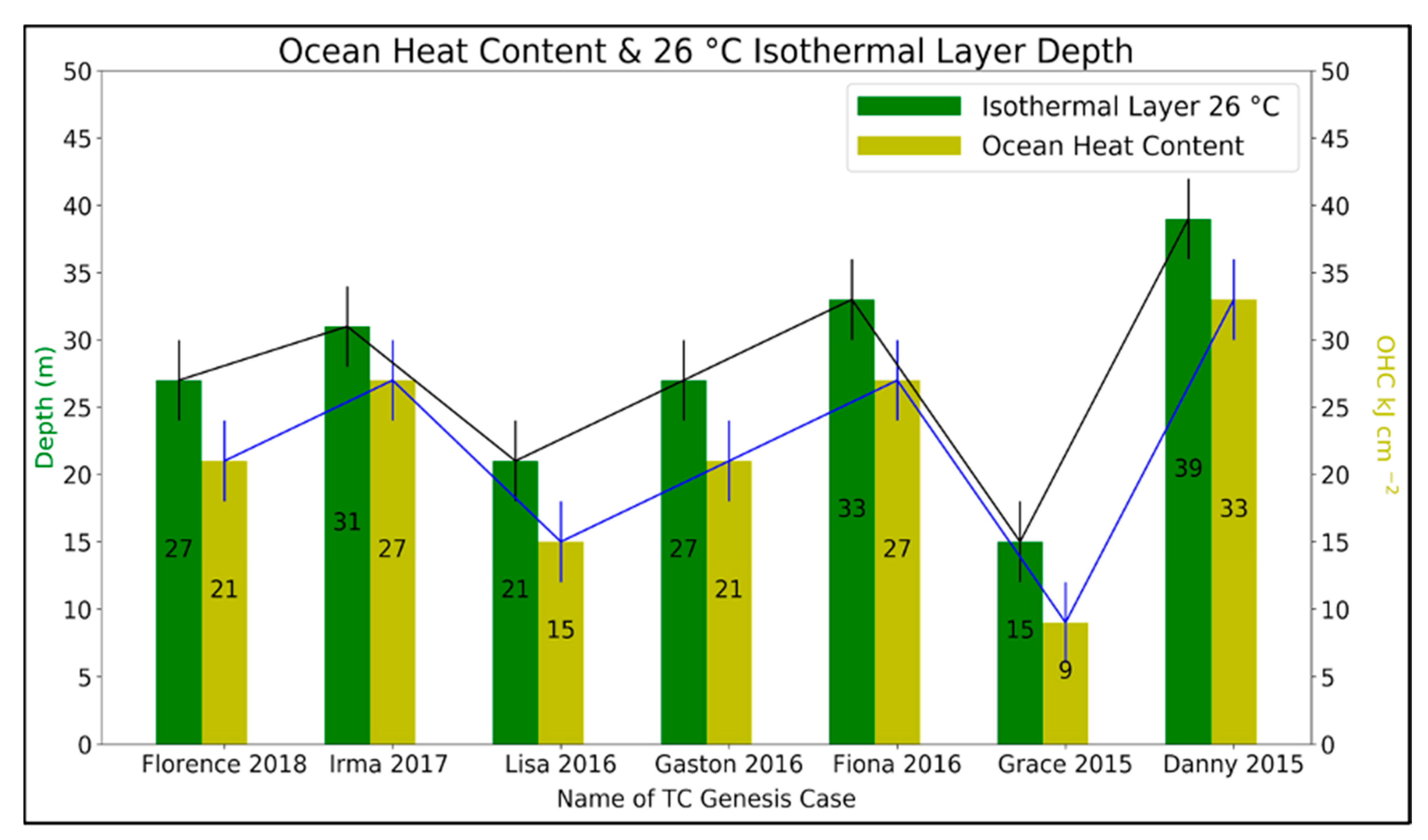
Observed results suggest the majority of the cases went through genesis in a 28–29 °C SST environment. In general, sea surface temperature anomalies (SSTA) were normally above average in the genesis region. Based on these observations, the surface environment was conducive for TC genesis to occur. However, an important understanding of the transfer of energy also needs to be evaluated during the time of genesis by the OHC (Figure 11). By understanding the SSTA to be above average, TC Matthew was not included in Figure 11 due circumstances that led to genesis not taking place.
The OHC value further exemplifies the essential fuel for the TC to develop in any favorable or unfavorable environment. For instance, TC Danny went through genesis under the highest OHC at 33 kJ cm−2 and managed to develop into a category 1 hurricane in 48 hrs. Additionally, it had the deepest isothermal layer depth (ISO) at 39 m below the surface (Figure 11).
A comparative analysis between the OHC and the ISO reveals the extent at which the energy was sustained within the ocean and at what depth. The domain 2 cases of Fiona and Danny showed a greater amount of OHC and a deeper ISO compared to the cases in domain 1 (Figure 11). In domain 1, TC Irma stood out to hold the deepest ISO and highest OHC and began rapidly intensifying after genesis occurred. However, TC Grace (2015), despite having the smallest ISO and lowest OHC at 9 kJ cm−2, still went through genesis and became a robust tropical storm in domain 1.
4. Discussion and Conclusions
The purpose of this study was to gather further insight into the relationship of probing dust aerosols and TC genesis in the Atlantic Ocean Basin. To obtain a quantitative value of observed dust concentration, the NASA CALIPSO satellite lidar at 532 nm wavelength was used. The MDR of the Atlantic Ocean Basin is conducive for TC development through various circumstances. As AEWs propagate into the Atlantic Ocean, dust aerosols are lofted into the atmosphere and carried over the basin. Visual observations from NASA’s MODIS/TERRA satellite display the evident dust outbreaks occurring with propagating AEWs. In total, eight (8) tropical cyclones were analyzed during genesis to understand the interaction of dust aerosols and supplementary environmental factors such as SSTs, VWS, and RH during the 2015–2018 time period.
Dust aerosol concentrations were different for each case resulting in varying impacts. The association with higher aerosol concentration amounts near the surface from the 0–1.75 km layer could be evidence of dense dust particulates (Table 2). Irma had the smallest total dust concentrations for both layers from 0~7 km−1sr−1 and underwent rapid intensification after genesis within a 24–48-hour time period (Table 2 and Table 3). Furthermore, the location of the dust plume was either parallel or ahead of the AEW for Grace, Lisa, Fiona, and Gaston with concentration in both layers from 6~12 km−1sr−1 (Table 2). This inference further supports the coinciding element of dust propagation with the TC activity in the MDR. It is important to note the impact dust aerosols have on the size distribution of the tropical systems forming in the MDR. For example, as seen on satellite imagery, Danny decreased in size and became a more organized tropical cyclone 24–48 h after dust interaction with higher aerosol concentrations compared to Grace which decrease in size with lower aerosol concentrations (Table 2). Interestingly, another feature that was noticed amongst the bulk of the cases was signs of rising aerosols as they approached the latitude of the genesis location. These near-surface aerosols could be entrained between the 1–3 km altitude level. However, there are also other environmental factors that could have limited the process of genesis to occur rather than the dust aerosols themselves. The case (i.e., Hurricane Jose 2017) that was discussed in Section 3.1 can be considered as an example for a condition of genesis with minimal dust aerosols but other favorable environmental variables. As observed from the official NHC Jose report [33], the system went on to become a tropical storm and a hurricane after genesis took place where minimal dust aerosols were associated during the genesis process, which was additionally validated by CALIPSO on 4 September 2017, 1 day before genesis [34]. This inference further supports the hypothesis that dust aerosols may not play a significant role in the inhibition of development and genesis when compared to the other cases that did have highly concentrated dust aerosols involved. It can be concluded that the common argument of suppression due to Saharan dust is not evident in these cases. No significant suppression of development occurred from the involvement of atmospheric dust aerosols as each case had gone through the genesis and developed into a tropical storm 24–48 h later (Table 3).
Overall, the VWS did not have a great negative influence on the cases during the time of genesis. A comparison amongst all cases shows the windshear within a 3-degree radius of the system primarily ranged from 0–10 ms−1 (Table 4). However, the environments ahead of some of those systems were becoming hostile. Generally, if the system consolidated early in domain 1 and had a defined circulation at the surface, the intensification process and genesis occurred in a more favorable environment. Danny and Fiona, which went through genesis in domain 2, faced a greater threat of windshear as the environment became less favorable.
The horizontal and vertical moisture profiles tell an intriguing story of how close the proximity of the SAL was and the depth it had with relation to the genesis location. The essential element of RH remained persistently moist amongst a 3 degree radius for each case. At the 1000 hPa level all cases ranged from 80–100% RH (Table 4). However, for Fiona, Lisa, Gaston, and Grace, RH can be seen dropping to a drier range at 50% (Table 4). In summary, the RH environmental conditions were favorable for cases such as Irma and Gaston but were neutral for cases such as Grace, Florence, and Danny. Finally, above average SST conditions were favorable for genesis to take place. The average SST amongst all cases was approximately 28 °C (Table 4). This sign from a climatology perspective suggests an increase in genesis activity to occur in the future with SST’s continuing to warm. The oceanic heat content comparison between all cases suggests Grace; a domain 1 case had the lowest OHC and ISO and still went through genesis. Domain 2 cases remained to have the highest OHC and deepest ISO compared to domain 1, which is expected due to domain 2 being further in the MDR (Figure 11).
Ultimately, observations from the CALIPSO satellite must be compared to aircraft observations and other satellite observations to quantify dust aerosol measurements in the Atlantic Ocean Basin. Additionally, it is imperative to expand future research on the dynamical and microphysical process of TC genesis with the relationship to dust aerosols using numerical models. These models should improve the scientific communities understanding about the direct and indirect influences. With this information, modeling capabilities can be improved, helping scientists assess and forecast the TCs as they propagate towards land from the MDR. This research provides further insight into the challenges associated with the relationship between dust aerosols and TC genesis. Lastly, this observational analysis can fund future research projects that can address scientific questions that can save millions of lives and prevent property damage from TCs.
Author Contributions
Conceptualization, S.C.; methodology, M.P., Q.T. and S.C.; software, M.P. and Q.T.; validation, M.P., S.C. and Q.T.; formal analysis, M.P.; investigation, M.P., Q.T. and S.C.; resources, M.P., Q.T. and S.C.; data curation, M.P. and Q.T.; writing—original draft preparation, M.P.; writing—review and editing, M.P. and S.C.; visualization, M.P.; supervision, S.C.; project administration, S.C.; funding acquisition, S.C. All authors have read and agreed to the published version of the manuscript.
Funding
This study was supported by the NASA MUREP grant (NNX15AQ02A), and NOAA/EPP Cooperative Agreement #NA16SEC4810006.
Institutional Review Board Statement
Not applicable.
Informed Consent Statement
Not applicable.
Data Availability Statement
The data presented in this study are available on request from the corresponding author.
Acknowledgments
We acknowledge the suppliers of datasets utilized in this research. We wish to express our appreciation to Paul Zechiel for the discussions and valuable suggestions. Comments and suggestions by anonymous reviewers were much appreciated.
Conflicts of Interest
The authors declare no conflict of interest.
References
- Gray, W.M. Global View of the Origin of Tropical Disturbances and Storms. Mon. Weather Rev. 1968, 96, 669–700. [Google Scholar] [CrossRef]
- Tompkins, C.; Chiao, S. Modeling studies of impacts from the Guinea Highlands in relation to tropical cyclogenesis along the West African coast. Meteorol. Atmos. Phys. 2012, 115, 51–72. [Google Scholar] [CrossRef]
- Schade, L.R. Tropical Cyclone Intensity and Sea Surface Temperature. J. Atmos. Sci. 2000, 57, 3122–3130. [Google Scholar] [CrossRef]
- Karloski, J.M. Evans, C. Seasonal Influences upon and Long-Term Trends in the Length of the Atlantic Hurricane Season. J. Clim. 2016, 29, 273–292. [Google Scholar] [CrossRef]
- Kossin, J.P. Is the North Atlantic hurricane season getting longer? Geophys. Res. Lett. 2008, 35, L23705. [Google Scholar] [CrossRef] [Green Version]
- Montgomery, M.T.; Farrell, B.F. Tropical Cyclone Formation. J. Atmos. Sci. 1993, 50, 285–310. [Google Scholar] [CrossRef] [Green Version]
- Demaria, M. The Effect of Vertical Shear on Tropical Cyclone Intensity Change. J. Atmos. Sci. 1996, 53, 2076–2088. [Google Scholar] [CrossRef] [Green Version]
- Holland, G.J. The Maximum Potential Intensity of Tropical Cyclones. J. Atmos. Sci. 1997, 54, 2519–2541. [Google Scholar] [CrossRef]
- Prospero, J.M.; Mayol-Bracero, O.L. Understanding the Transport and Impact of African Dust on the Caribbean Basin. Bull. Am. Meteor. Soc. 2013, 94, 1329–1337. [Google Scholar] [CrossRef]
- Jones, C.; Mahowald, N.; Luo, C. The Role of Easterly Waves on African Desert Dust Transport. J. Clim. 2003, 16, 3617–3628. [Google Scholar] [CrossRef] [Green Version]
- Lau, K.M.; Kim, K.M. Cooling of the Atlantic by Saharan dust. Geophys. Res. Lett. 2007, 34, L23811. [Google Scholar] [CrossRef] [Green Version]
- Sun, D.; Lau, K.; Kafatos, M. Contrasting the 2007 and 2005 hurricane seasons: Evidence of possible impacts of Saharan dry air and dust on tropical cyclone activity in the Atlantic basin. Geophys. Res. Lett. 2008, 35, L15405. [Google Scholar] [CrossRef] [Green Version]
- Jenkins, G.S.; Pratt, A.S.; Heymsfield, A. Possible linkages between Saharan dust and tropical cyclone rain band invigoration in the eastern Atlantic during NAMMA-06. Geophys. Res. Lett. 2008, 35, L08815. [Google Scholar] [CrossRef] [Green Version]
- Amiri-Farahani, A.; Allen, R.J.; Neubauer, D.; Lohmann, U. Impact of Saharan dust on North Atlantic marine stratocumulus clouds: Importance of the semidirect effect. Atmos. Chem. Phys. 2017, 17, 6305–6322. [Google Scholar] [CrossRef] [Green Version]
- Bretl, S.; Reutter, P.; Raible, C.C.; Ferrachat, S.; Poberaj, C.S.; Revell, L.E.; Lohmann, U. The influence of absorbed solar radiation by Saharan dust on hurricane genesis. J. Geophys. Res. Atmos. 2015, 120, 1902–1917. [Google Scholar] [CrossRef] [Green Version]
- Dunion, J.P.; Velden, C.S. The Impact of the Saharan Air Layer on Atlantic Tropical Cyclone Activity. Bull. Am. Meteor. Soc. 2004, 85, 353–366. [Google Scholar] [CrossRef] [Green Version]
- Grogan, D.F.; Nathan, T.R.; Chen, S. Effects of Saharan Dust on the Linear Dynamics of African Easterly Waves. J. Atmos. Sci. 2016, 73, 891–911. [Google Scholar] [CrossRef]
- Zhang, H.; McFarquhar, G.M.; Cotton, W.R.; Deng, Y. Direct and indirect impacts of Saharan dust acting as cloud condensation nuclei on tropical cyclone eyewall development. Geophys. Res. Lett. 2009, 36, L06802. [Google Scholar] [CrossRef] [Green Version]
- Braun, S.A. Reevaluating the Role of the Saharan Air Layer in Atlantic Tropical Cyclogenesis and Evolution. Mon. Weather Rev. 2010, 138, 2007–2037. [Google Scholar] [CrossRef]
- Sauter, K.; L’Ecuyer, T.S. Observational evidence for the vertical redistribution and scavenging of Saharan dust by tropical cyclones. Geophys. Res. Lett. 2017, 44, 6421–6430. [Google Scholar] [CrossRef]
- Fritz, C.; Wang, Z. A Numerical Study of the Impacts of Dry Air on Tropical Cyclone Formation: A Development Case and a Nondevelopment Case. J. Atmos. Sci. 2013, 70, 91–111. [Google Scholar] [CrossRef]
- Braun, S.A.; Sippel, J.A.; Shie, C.; Boller, R.A. The Evolution and Role of the Saharan Air Layer during Hurricane Helene (2006). Mon. Wea. Rev. 2013, 141, 4269–4295. [Google Scholar] [CrossRef] [Green Version]
- Tackett, J.L.; Winker, D.M.; Getzewich, B.J.; Vaughan, M.A.; Young, S.A.; Kar, J. CALIPSO lidar level 3 aerosol profile product: Version 3 algorithm design. Atmos. Meas. Tech. 2018, 11, 4129–4152. [Google Scholar] [CrossRef] [PubMed] [Green Version]
- NASA/LARC/SD/ASDC. CALIPSO Lidar Level 2 Aerosol Profile, V4-20 [Data set]. NASA Langley Atmospheric Science Data Center DAAC. 2018. Available online: https://0-doi-org.brum.beds.ac.uk/10.5067/CALIOP/CALIPSO/LID_L2_05KMAPRO-STANDARD-V4-20 (accessed on 15 August 2018).
- Kar, J.; Vaughan, M.A.; Lee, K.-P.; Tackett, J.L.; Avery, M.A.; Garnier, A.; Getzewich, B.J.; Hunt, W.H.; Josset, D.; Liu, Z.; et al. CALIPSO lidar calibration at 532 nm: Version 4 nighttime algorithm. Atmos. Meas. Tech. 2018, 11, 1459–1479. [Google Scholar] [CrossRef] [PubMed] [Green Version]
- Liu, Z.; Vaughan, M.; Winker, D.; Kittaka, C.; Getzewich, B.; Kuehn, R.; Omar, A.; Powell, K.; Trepte, C.; Hostetler, C. The CALIPSO Lidar Cloud and Aerosol Discrimination: Version 2 Algorithm and Initial Assessment of Performance. J. Atmos. Oceanic Technol. 2009, 26, 1198–1213. [Google Scholar] [CrossRef]
- Young, S.A.; Vaughan, M.A.; Garnier, A.; Tackett, J.L.; Lambeth, J.D.; Powell, K.A. Extinction and optical depth retrievals for CALIPSO’s Version 4 data release. Atmos. Meas. Tech. 2018, 11, 5701–5727. [Google Scholar] [CrossRef] [Green Version]
- European Centre for Medium-Range Weather Forecasts. 2009, Updated Monthly. ERA-Interim Project. Research Data Archive at the National Center for Atmospheric Research, Computational and Information Systems Laboratory. Available online: https://0-doi-org.brum.beds.ac.uk/10.5065/D6CR5RD9 (accessed on 13 April 2020).
- European Centre for Medium-Range Weather Forecasts. 2019, Updated Monthly. ERA5 Reanalysis (0.25 Degree Latitude-Longitude Grid). Research Data Archive at the National Center for Atmospheric Research, Computational and Information Systems Laboratory. Available online: https://0-doi-org.brum.beds.ac.uk/10.5065/BH6N-5N20 (accessed on 3 June 2020).
- Reynolds, R.; Thomas, W.; Smith, M.; Liu, C.; Dudley, B.; Chelton, K.; Casey, S.; Michael, G. Daily High-Resolution-Blended Analyses for Sea Surface Temperature. J. Clim. 2007, 20, 5473–5496. [Google Scholar] [CrossRef]
- Donahue, D. US DOC/NOAA > National Environmental Satellite, Data, and Information Service (NESDIS). Satellite Ocean Heat Content Suite. [Indicate Subset Used]. NOAA National Centers for Environmental Information. Dataset. 2015. Available online: https://www.ncei.noaa.gov/archive/accession/NESDIS-OHC (accessed on 25 July 2020).
- 2018 Atlantic Hurricane Season Official NHC Reports. Available online: https://www.nhc.noaa.gov/data/tcr/index.php?season=2018&basin=atl (accessed on 27 July 2021).
- 2017 Atlantic Hurricane Season Official NHC Reports. Available online: https://www.nhc.noaa.gov/data/tcr/index.php?season=2017&basin=atl (accessed on 27 July 2021).
- Trepte, C.R. 4 September 2017 CALIPSO Pass. 2021. Available online: https://www-calipso.larc.nasa.gov/products/lidar/browse_images/show_v4_detail.php?s=production&v=V4-10&browse_date=2017-09-04&orbit_time=03-31-29&page=2&granule_name=CAL_LID_L1-Standard-V4-10.2017-09-04T03-31-29ZN.hdf (accessed on 27 July 2021).
- 2015 Atlantic Hurricane Season Official NHC Reports. Available online: https://www.nhc.noaa.gov/data/tcr/index.php?season=2015&basin=atl (accessed on 27 July 2021).
- 2016 Atlantic Hurricane Season Official NHC Reports. Available online: https://www.nhc.noaa.gov/data/tcr/index.php?season=2016&basin=atl (accessed on 27 July 2021).
Figure 1.
Region of focus split into two domains for genesis. Shaded color contours represent height above sea level in meters.
Figure 1.
Region of focus split into two domains for genesis. Shaded color contours represent height above sea level in meters.

Figure 2.
TERRA/MODIS visual satellite imagery obtained from NASA Worldview. The red line represents CALIPSO Satellite track on the given satellite imagery date. (a) Florence, (b) Irma, (c) Matthew, (d) Lisa, (e) Gaston, (f) Fiona, (g) Grace, and (h) Danny.
Figure 2.
TERRA/MODIS visual satellite imagery obtained from NASA Worldview. The red line represents CALIPSO Satellite track on the given satellite imagery date. (a) Florence, (b) Irma, (c) Matthew, (d) Lisa, (e) Gaston, (f) Fiona, (g) Grace, and (h) Danny.

Figure 3.
CALIPSO Satellite 532 nm Attenuated Backscatter plot from surface to 6 km altitude. The black dashed line represents the AEW/TC location in latitude. Threshold set to 0.001–0.01 km−1sr−1. (a) Florence, (b) Irma, (c) Matthew, (d) Lisa, (e) Gaston, (f) Fiona, (g) Grace, and (h) Danny.
Figure 3.
CALIPSO Satellite 532 nm Attenuated Backscatter plot from surface to 6 km altitude. The black dashed line represents the AEW/TC location in latitude. Threshold set to 0.001–0.01 km−1sr−1. (a) Florence, (b) Irma, (c) Matthew, (d) Lisa, (e) Gaston, (f) Fiona, (g) Grace, and (h) Danny.

Figure 4.
CALIPSO Satellite 532 nm Attenuated Backscatter anomaly plot from surface to 1.756 km altitude. Threshold set to −0.01–0.01 km−1sr−1. (a) Florence, (b) Irma, (c) Matthew, (d) Lisa, (e) Gaston, (f) Fiona, (g) Grace, and (h) Danny.
Figure 4.
CALIPSO Satellite 532 nm Attenuated Backscatter anomaly plot from surface to 1.756 km altitude. Threshold set to −0.01–0.01 km−1sr−1. (a) Florence, (b) Irma, (c) Matthew, (d) Lisa, (e) Gaston, (f) Fiona, (g) Grace, and (h) Danny.

Figure 5.
CALIPSO Satellite 532 nm Attenuated Backscatter plot from surface to 5 km altitude for (a) August, and (b) September average from (2015–2018). The black dashed line represents the AEW/TC location in latitude. There are two thresholds set, first to 0.001–0.01 km−1sr−1 and secondly, 0.01–0.05 km−1sr−1 to detect the higher near surface TAB.

Figure 6.
CALIPSO Satellite 532 nm Attenuated Backscatter plot from surface to 5 km altitude. Threshold set to 0.005–0.05 km−1sr−1. The pink dashed line represents the AEW/TC location in latitude. (a) Florence, (b) Irma, (c) Matthew, (d) Lisa, (e) Gaston, (f) Fiona, (g) Grace, and (h) Danny.
Figure 6.
CALIPSO Satellite 532 nm Attenuated Backscatter plot from surface to 5 km altitude. Threshold set to 0.005–0.05 km−1sr−1. The pink dashed line represents the AEW/TC location in latitude. (a) Florence, (b) Irma, (c) Matthew, (d) Lisa, (e) Gaston, (f) Fiona, (g) Grace, and (h) Danny.

Figure 7.
The total amount of TAB for each CALIPSO pass from 10–20 N latitude.

Figure 8.
ERA-Interim magnitude vertical windshear representation with direction. Green circle indicates location of the TC, red arrows (850 hPa wind), yellow arrows (250 hPa wind), and black arrows (shear from 250–850 hPa). (a) Florence, (b) Irma, (c) Matthew, (d) Lisa, (e) Gaston, (f) Fiona, (g) Grace, and (h) Danny.

Figure 9.
ERA-Interim 700 hPa relative humidity representation with 1000 hPa wind barbs. Red circle indicates the location of/TC. (a) Florence, (b) Irma, (c) Matthew, (d) Lisa, (e) Gaston, (f) Fiona, (g) Grace, and (h) Danny.
Figure 9.
ERA-Interim 700 hPa relative humidity representation with 1000 hPa wind barbs. Red circle indicates the location of/TC. (a) Florence, (b) Irma, (c) Matthew, (d) Lisa, (e) Gaston, (f) Fiona, (g) Grace, and (h) Danny.

Figure 10.
ERA-Interim relative humidity cross-section representation at all levels. Upper right corner depicts a cross section slice location and 700 hPa RH. Violet circle and dashed line indicate location of the AEW/TC. (a) Florence, (b) Irma, (c) Matthew, (d) Lisa, (e) Gaston, (f) Fiona, (g) Grace, and (h) Danny.

Figure 11.
Case comparison of ocean heat content and isothermal layer depth at 26 °C using NESDIS’s Satellite Ocean Heat Suite (SOHS).
Figure 11.
Case comparison of ocean heat content and isothermal layer depth at 26 °C using NESDIS’s Satellite Ocean Heat Suite (SOHS).


Table 1.
Categorizes each case with its CALIPSO Pass Date, Genesis (TD) Date (i.e., NHC classified system as a TD), Days Between Pass & Genesis Date, and Domain.
Table 1.
Categorizes each case with its CALIPSO Pass Date, Genesis (TD) Date (i.e., NHC classified system as a TD), Days Between Pass & Genesis Date, and Domain.
| Name | Year | CALIPSO Pass Date | Genesis (TD) Date | Days Between Pass & Genesis Date | Domain |
|---|---|---|---|---|---|
| Florence | 2018 | 31 August 2018 | 31 August 2018 | 0 | 1 |
| Irma | 2017 | 29 August 2017 | 30 August 2017 | −1 | 1 |
| Jose | 2017 | 4 September 2017 | 5 September 2017 | −1 | 2 |
| Gaston | 2016 | 20 August 2016 | 22 August 2016 | −2 | 1 |
| Fiona | 2016 | 17 August 2016 | 16 August 2016 | +1 | 2 |
| Lisa | 2016 | 17 September 2016 | 19 September 2016 | −2 | 1 |
| Matthew | 2016 | 24 September 2016 | 28 September 2016 | −4 | NA |
| Grace | 2015 | 6 September 2015 | 5 September 2015 | +1 | 1 |
| Danny | 2015 | 17 August 2015 | 18 August 2016 | −1 | 2 |
Table 2.
Categorizes each case with its Genesis (TD) Date and TAB concentration.
| Name | Year | CALIPSO Pass Date | Genesis (TD) Date | Total TAB 0–1.75 km km−1sr−1 | Total TAB 1.75–6 km km−1sr−1 |
|---|---|---|---|---|---|
| Florence | 2018 | 31 August 2018 | 31 August 2018 | 6.63 | 3.47 |
| Irma | 2017 | 29 August 2017 | 30 August 2017 | 4.52 | 0.94 |
| Gaston | 2016 | 20 August 2016 | 22 August 2016 | 11.19 | 7.80 |
| Fiona | 2016 | 17 August 2016 | 16 August 2016 | 12.75 | 6.16 |
| Lisa | 2016 | 17 September 2016 | 19 September 2016 | 7.44 | 8.86 |
| Matthew | 2016 | 24 September 2016 | 28 September 2016 | 19.20 | 12.73 |
| Grace | 2015 | 6 September 2015 | 5 September 2015 | 10.49 | 6.70 |
| Danny | 2015 | 17 August 2015 | 18 August 2015 | 10.61 | 28.18 |
Table 3.
Displays the Genesis (TD) Date, CALIPSO pass date windspeed, +24 h windspeed, and +48 h windspeed. Data retrieved from Official NHC Reports [32,33,35,36].
| Name | Genesis (TD) Date | CALIPSO Pass Date 03Z—04Z Rounded to 06Z | During CALIPSO Pass Windspeed Intensity | +24 h Windspeed in kts from CALIPSO Pass | +48 h Windspeed in kts from CALIPSO Pass |
|---|---|---|---|---|---|
| Florence | 31 August 2018 | 31 August 2018 | 30 kts | 35 kts (01/06Z) | 50 kts (02/06Z) |
| Irma | 30 August 2017 | 29 August 2017 | <20 kts | 35 kts (30/06Z) | 65 kts (31/06Z) |
| Gaston | 22 August 2016 | 20 August 2016 | <20 kts | 20 kts (21/12Z) | 30 kts (22/12Z) |
| Fiona | 16 August 2016 | 17 August 2016 | 30 kts | 40 kts (18/06Z) | 45 kts (19/06Z) |
| Lisa | 19 September 2016 | 17 September 2016 | <20 kts | <25 kts (19/06Z) | 30 kts (20/06Z) |
| Matthew | 28 September 2016 | 24 September 2016 | NA | NA | NA |
| Grace | 5 September 2015 | 6 September 2015 | 45 kts | 45 kts (07/06Z) | 35 kts (08/06Z) |
| Danny | 18 August 2015 | 17 August 2015 | 25 kts | 30 kts (18/06Z) | 45 kts (19/06Z) |
Table 4.
Categorizes each case with its date and environmental conditions.
| Name | Genesis (TD) Date | SST °C | VWS m/s | RH850% | RH700% |
|---|---|---|---|---|---|
| Florence | 31 August 2018 | 27–28 | 5–10 | 80–100 | 50–80 |
| Irma | 30 August 2017 | 27 | 5 | 80–100 | 70–85 |
| Gaston | 22 August 2016 | 28–29 | 5–10 | 80–100 | 75–90 |
| Fiona | 16 August 2016 | 28–29 | 5 | 90–100 | 30–80 |
| Lisa | 19 September 2016 | 27 | 0 | 90–100 | 50–90 |
| Matthew | NA | 28 | 10–18 | 90–100 | 55–85 |
| Grace | 5 September 2015 | 28–29 | 5 | 90–100 | 60–90 |
| Danny | 18 August 2015 | 28–29 | 5 | 90–100 | 60–75 |
Publisher’s Note: MDPI stays neutral with regard to jurisdictional claims in published maps and institutional affiliations. |
© 2021 by the authors. Licensee MDPI, Basel, Switzerland. This article is an open access article distributed under the terms and conditions of the Creative Commons Attribution (CC BY) license (https://creativecommons.org/licenses/by/4.0/).
Share and Cite
MDPI and ACS Style
Patel, M.; Chiao, S.; Tan, Q. An Observational Study of Aerosols and Tropical Cyclones over the Eastern Atlantic Ocean Basin for Recent Hurricane Seasons. Atmosphere 2021, 12, 1036. https://0-doi-org.brum.beds.ac.uk/10.3390/atmos12081036
AMA Style
Patel M, Chiao S, Tan Q. An Observational Study of Aerosols and Tropical Cyclones over the Eastern Atlantic Ocean Basin for Recent Hurricane Seasons. Atmosphere. 2021; 12(8):1036. https://0-doi-org.brum.beds.ac.uk/10.3390/atmos12081036
Chicago/Turabian StylePatel, Mohin, Sen Chiao, and Qian Tan. 2021. "An Observational Study of Aerosols and Tropical Cyclones over the Eastern Atlantic Ocean Basin for Recent Hurricane Seasons" Atmosphere 12, no. 8: 1036. https://0-doi-org.brum.beds.ac.uk/10.3390/atmos12081036
Note that from the first issue of 2016, this journal uses article numbers instead of page numbers. See further details here.