
Impact of Radio Occultation Data on the Prediction of Typhoon Haishen (2020) with WRFDA Hybrid Assimilation


1
GPS Science and Application Research Center, National Central University, Taoyuan City 320317, Taiwan
2
Department of Atmospheric Sciences, National Central University, Taoyuan City 320317, Taiwan
*
Author to whom correspondence should be addressed.
Atmosphere 2021, 12(11), 1397; https://0-doi-org.brum.beds.ac.uk/10.3390/atmos12111397
Submission received: 15 September 2021
/
Revised: 15 October 2021
/
Accepted: 22 October 2021
/
Published: 25 October 2021
(This article belongs to the Special Issue Toward Improvement of Typhoon/Hurricane Prediction with Better-Initialization and Higher-Resolution Models)
Abstract
:FORMOSAT-7/COSMIC-2 (FS7/C2) satellite was successfully launched in June 2019. The satellite provides about 5000 radio occultation (RO) soundings daily over the tropical and partial subtropical regions. Such plentiful RO soundings with high accuracy and vertical resolution could be used to improve model initial analysis for typhoon prediction. In this study, assimilation experiments with and without the RO data were conducted with the WRFDA hybrid system for the prediction of Typhoon Haishen (2020). The experimental results show a remarkable improvement in typhoon track prediction with RO data assimilation, especially when using a nonlocal refractivity operator. Results in cycling DA and forecast are analyzed and verified for the RO data impact. Diagnostics of potential vorticity (PV) tendency budget helps explain the typhoon translation induced by different physical processes in the budget. The typhoon translation is essentially dominated by horizontal PV advection, but the track deviation can increase due to the vertical PV advection with opposite effects in the absence of RO data. Sensitivity experiments for different model initial times, physics schemes, and RO observation amounts show positive RO data impacts on typhoon prediction, mainly contributed from FS7. Complementary, an improved forecast of Typhoon Hagupit (2020) is also illustrated for the RO data impact.
1. Introduction
The northwestern Pacific basin is one of the regions where tropical cyclones are active, and the tropical cyclones or typhoons are usually accompanied by strong wind speeds and heavy precipitation, which could result in human life and economic damages. The Global Navigation Satellite System (GNSS) Radio Occultation (RO) could be useful for detecting atmospheric information over the ocean. In the past decade, many studies have shown the positive influences of GNSS RO data in multiple ways, e.g., climatological monitoring, numerical weather predictions (NWP), and a reliable calibrator for other observations, etc. [1]. In addition, GNSS RO data have been operationally used in several weather prediction centers (e.g., [2,3,4,5,6]). The FORMOsa SATellite mission-7/Constellation Observing System for the Meteorology, Ionosphere, and Climate mission-2 (FORMOSAT-7/COSMIC-2, hereafter FS7/C2), which is a follow-on mission of FORMOSAT-3/COSMIC (FS3/C), was launched on 25 June 2019, and it now can provide more than 5000 RO soundings per day within the ±45° latitudinal region. The FS7/C2 data provide not only a larger data amount but also penetrate farther to near the surface than the FS3/C data, and qualities of both data are comparable (e.g., [7,8,9]). For example, Ho et al. [8] compared the FORMOSAT-7/COSMIC-2 RO data and the radiosonde observations, and the mean difference and standard deviation (STD) of the refractivity were about 0.34% and 1.84%, respectively. A relatively larger STD is present in the lower troposphere but decreases significantly in the upper troposphere with a nearly constant STD of about 1% at 30 km. The STD variation of the refractivity compared to ECMWF global analysis is similar, as shown by Schreiner et al. [7]. Anthes et al. [10] also showed the good quality of FS7/C2 RO data in a hurricane event with an extremely moist atmosphere. The plentiful profiling observations at the lower troposphere over the ocean could be useful to derive the atmospheric moisture for use in the NWP. From an Observing System Simulation Experiment, Cucurull and Casey [11] found significant positive impacts on mass and wind fields with FS7/C2 RO data assimilation. About one year after the launch, the FS7/C2 RO data started to be used operationally in some official weather centers. For example, the RO data were implemented in both European Centre for Medium-Range Weather Forecasts (ECMWF) and National Centers for Environmental Prediction (NCEP) starting in March and May 2020, respectively. The Central Weather Bureau (CWB) in Taiwan also implemented the FS7/C2 RO data in their operating system in the later month of the year (Sep. 2020). Early results of the assessment of the FS7/C2 RO data in the NWP system can be found in Healy [12], Shao et al. [13], and Lien et al. [14], and they showed generally positive to neutral impacts and a significant effect in the tropical region.
Many investigations have been conducted for analyses of tropical cyclones by using the GNSS RO data. For example, Bonafoni et al. [15] reviewed GNSS relevant research involving space-based RO data and ground-based products in 2000–2019. The first and second ranks of the topics are the convective storms in 40% and tropical cyclones in 25%, while the tropical cyclone is the most popular topic for the space-based RO study. The GNSS RO data are important for typhoon predictions because of their high accuracy and quality and sparse observations available over the ocean. Some papers have shown promising positive impacts on tropical cyclogenesis (e.g., [16]) and typhoon prediction (e.g., [17,18,19]) over the northwestern Pacific Ocean. Chen et al. [19] assessed the RO data impacts on 11 typhoons over the northwestern Pacific in 2008–2010 and found an averaged 5% improvement in 72-h track prediction. These studies used a three-dimensional variation (3DVAR) DA approach.
For the data assimilation (DA), two DA methods are mostly used in the community, i.e., variational-based or ensemble-based assimilations. Recently, a hybrid DA algorithm has been proposed to improve the analysis by combining both methods (e.g., [20,21,22]). Schwartz et al. [23] used the 3DVAR and hybrid variational-ensemble data assimilation for the forecasts of typhoon tracks, and they found that the hybrid method produced superior predictions than the 3DVAR. For investigating the RO data impact, the hybrid DA method, called 3DEnVar, is adopted for this study. The Weather Research and Forecasting (WRF) model is equipped with a data assimilation system (called WRFDA) that provides several options for the DA methods. The hybrid scheme (3DEnVar) in WRFDA that combines 3DVAR and ensemble Kalman filter is adopted for RO data assimilation in the impact study.
Typhoon Haishen was a super typhoon over the Western North Pacific in 2020. It was a tropical depression (TD) in northeastern Guam on 1 September 2020. The TD went southwestward and then turned clockwise in northwestward with rapid intensification. At 1200 UTC on 4 September, the central sea-level pressure of the typhoon reached a minimum of 910 hPa, as reported by Japan Meteorological Agency (JMA). It continued to move northwestward toward Korea and Japan. In the meanwhile, a clear eye embedded in a rather symmetrical structure was visible on satellite imagery. On 5 September, Typhoon Haishen kept moving north–northwestward and started to weaken. Later on, Typhoon Haishen (2020) made landfall on Japan and South Korea with a category-2 intensity.
Since hybrid assimilation with FS7 RO data is still not well illustrated in literature, we aim to investigate the FS7 RO data impact on the typhoon prediction and understand the dynamic mechanism of the typhoon track with the intention to improve the knowledge base. The impact of FS7/C2 RO data on the prediction of Typhoon Haishen (2020) is investigated. Experiments with and without RO data assimilation are conducted to identify the impacts of RO data on the model initial analyses and ensuing predictions. The numerical model and GNSS RO data are introduced in Section 2. The simulated results with verification are discussed in Section 3, where the potential vorticity (PV) tendency budget is diagnosed to help explain the RO data impacts on track prediction. Sensitivity experiments regarding model initial times, physics schemes, and RO observation amounts are given in Section 4. We also show a complimentary case of Typhoon Hagupit (2020) to illustrate the positive RO data impacts on track prediction in this section. The conclusions are finally given in Section 5.
2. The Numerical Model and GNSS RO Data
2.1. Hybrid WRFDA System and Model Configurations
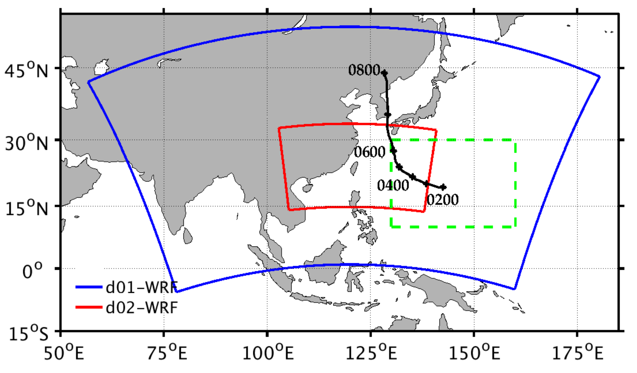
The WRF Model (WRF-ARW, [24]) is fully compressible and non-hydrostatic, and it has been widely used in the research community and many forecast centers for weather prediction. In this study, we used two model domains with horizontal resolutions of 15 km and 3 km, respectively (Figure 1), and the grid cells were 662 × 386 for the outermost domain and 1161 × 676 for the inner domain. The NCEP Final operational global analysis (FNL) [25] at a horizontal resolution of 0.25° × 0.25° was used to provide the initial and lateral boundary conditions for WRF. For the vertical domain, 52 layers with a model top of 20 hPa were used. The model physics schemes included the Goddard 4-ice microphysics scheme [26,27], the Kain–Fritsch cumulus parameterization [28], the Yonsei University (YSU) planetary boundary layer (PBL) parameterization scheme [29], and a new version of the Rapid Radiative Transfer Model (RRTMG) [30] for the radiation effects. The model domains and configurations are the same as in the CWB’s regional operational system. The forecasts in the outer domain will be used for all discussion later.
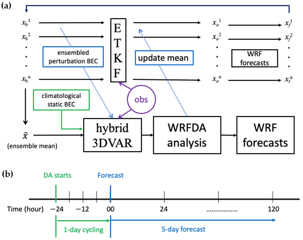
The DA system equipped with WRF is the WRFDA [31], which provides multiple options for the data analysis, including three- and four-dimensional variational DA (3D-Var and 4D-Var) [32,33], ensemble transform Kalman filter (ETKF) [34,35], and hybrid DA algorithms (3DEnVar and 4DEnVar) which combine both climatological statistics and flow-dependent background error covariances (BEC) [21,36]. In this study, we used the 3DEnVar hybrid system. The ensemble members were generated by WRFDA to calculate 32 ensemble perturbations for the ETKF in this study. The ensemble-based flow-dependent BEC can be estimated by the 6-h ensemble forecasts. For the hybrid DA, BEC can be obtained by weighting the flow-dependent BEC by 75% and the static BEC by 25%, following Hamill et al. [37] and Kleist et al. [38]. All the ensemble members and hybrid variational DA used the same model resolution. The WRF-ARW and WRFDA models in version 4.2 were adopted in this study, and the detailed descriptions of both the WRF model and WRFDA can be found in https://www.mmm.ucar.edu/weather-research-and-forecasting-model (accessed on 8 July 2020) [39].
2.2. The GNSS RO Forward Operators in the WRFDA
Both GNSS RO refractivity and bending angle are often used in data assimilation systems for operations and research (e.g., [3,4,5,6,16,40,41]). Before ingesting these RO variables into model states, a corresponding forward operator is needed to connect RO observations and model variables. Herein, the RO refractivity (N) can be related to several atmospheric variables [42], such as
where P is the pressure of the atmosphere in hPa, T the temperature in K, and q the specific humidity in kg kg−1. Both the refractivity and bending angle were derived under the assumption of spherical symmetry, as two local operators. To consider the influence of horizontal atmospheric variations, the nonlocal refractivity operator was proposed by Sokolovskiy et al. [43], and the observable, called pseudo excess phase (S), was implemented in the WRFDA system [17,44]. The pseudo excess phase takes the integration of refractivity along the ray path, which would be more beneficial to assimilation for an inhomogeneous atmosphere. It can be defined as
where l is the ray path (usually simplified by an approximately straight line). Chen et al. [16] compared the local and nonlocal refractivity operators in a single-sounding assimilation by using WRF 3DVAR. From their comparisons, the two RO operators showed similar patterns in the analysis increments, but the nonlocal refractivity exhibited an elliptical distribution of the increment along the ray path, whereas the local operator showed a more circular distribution of the increment. The nonlocal operator in a 3DVAR system has shown an outperformance in the prediction of tropical cyclogenesis compared to the local operator [16].
The local refractivity operator for the GNSS RO data assimilation is currently used in the CWB operational weather prediction. In this study, we thus compared the two operators, i.e., local and nonlocal refractivity operators, in the hybrid WRFDA system. That is the first time the two operators in a hybrid DA system have been compared for the RO data impact on typhoon predictions. The observational error and quality control criteria for the two RO operators use the default settings in the WRFDA. The observational errors for local refractivity vary with latitude and altitude. The percentage errors are 2.5% and 1.5% near the surface for a sounding located at the equator and pole, respectively. Then, the observational errors decrease to 0.3% at the height of 12 km. For the nonlocal refractivity operator, the observational error is about 1% near the surface and decreases to about 0.2% near the troposphere from Chen et al. [17]. More details about the observational error for GNSS RO in the WRFDA can be found in Chen et al. [16].
2.3. Experimental Design
In the beginning, the NCEP global analysis at 0600 UTC 1 September 2020 was adopted as the initial condition, and then a 6-h forecast was conducted by the WRF model. The 6-h forecast was then perturbed by the function RANDOMCV in WRFDA, which adds random noises to the analysis in the control variable space. This perturbed procedure results in 32 ensemble members, and the ensemble mean was adopted as a first guess for the hybrid 3DVAR. In the meanwhile, a flow-dependent BEC was also derived from the 32 ensemble members. After the minimization of the hybrid 3DVAR, the analysis was then adopted to replace the ensemble mean after the ETKF process (Figure 2a), i.e., the mean-updated process restricts the two assimilation systems (ETKF and 3DEnVar) to have a similar synoptic state, and they will not depart greatly after a long-period DA cycling. For this typhoon case, the DA process started from 1200 UTC 1 September, and continuous DA cycling with a 6-h interval was carried out. After 1-day DA cycling, a 5-day WRF simulation was conducted, i.e., 1200 UTC 2–7 September (Figure 2b). Three experiments (Table 1) were conducted to investigate the RO data impact. One experiment was conducted with assimilation with the convectional data and satellite retrieved wind only, denoted by GTS, which was the baseline control experiment (CTL). The other two experiments were the assimilation runs with the additional GNSS RO data using the local refractivity operator (hereafter REF) or the nonlocal pseudo excess phase operator (hereafter EPH).
During the 1-day period, there were about one thousand GNSS RO data within the outer domain, as shown in Figure 3. The RO soundings included FORMOSAT-7/COSMIC-2, Meteorological Operational satellites (MetOp), Korea Multi-Purpose Satellite-5 (KOMPSAT-5), and Spanish Earth Observation satellite (PAZ). For the total 959 RO profiles, there were more than seven hundred data from FORMOSAT-7, indicating that the FS7/C2 data were the major contribution (about 75%) to the RO soundings. Although the coverage of FS7 RO soundings was in the latitude of ±45 degrees, our outer model domain was located inside this region, and thus, the retrieved FS7/C2 data information (from red points in Figure 3a) influenced the entire domain. Figure 3b shows the vertical variation of the total amounts of accumulated RO soundings at each DA cycle. The data amounts decreased from 6-km height to lower altitudes, and the minimum and maximum amounts were about 80 and 170 near the surface, respectively. At higher altitudes over 5 km, the RO data amounts during the 1-day period were about 130–250.
3. Simulated Results and Discussion
3.1. Initial Analysis
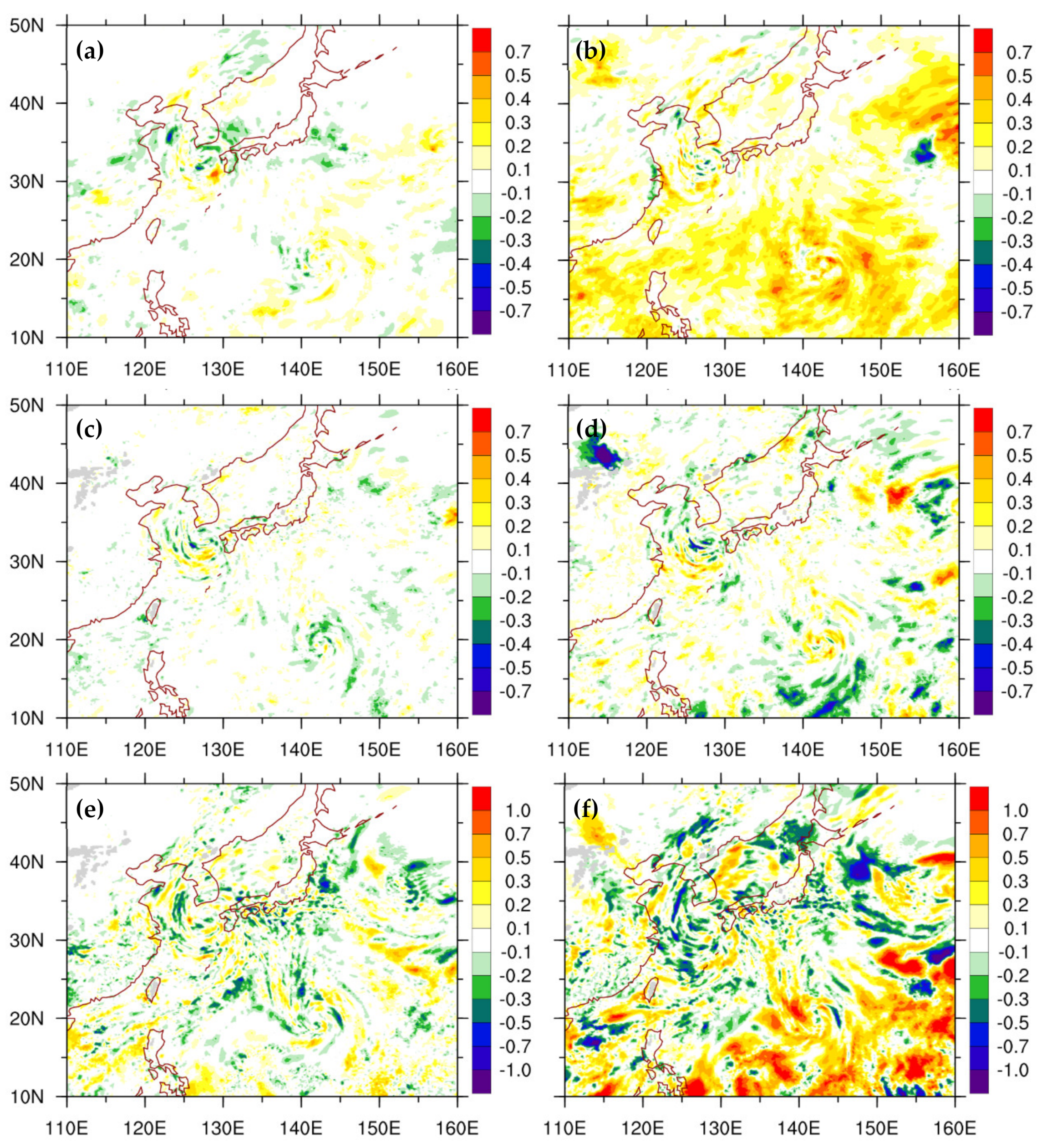
After the first DA cycle, the differences between the assimilation with and without GNSS RO data, i.e., REF-GTS and EPH-GTS, presented similar patterns in temperature and moisture analyses (Figure 4). At 500 hPa, both RO experiments (REF and EPH) provided a warmer temperature than GTS over the storm region of Typhoon Haishen. Over most of the northwestern Pacific Ocean, the RO data assimilation tended to a warm atmosphere at mid-troposphere (Figure 4a,b) and colder at the lower troposphere (Figure 4c,d). At the lower troposphere (850 hPa), they had similar patterns, but EPH showed a larger difference in the water vapor mixing ratio compared to GTS. Generally, both EPH and REF showed comparable differences relative to GTS in temperature but with relatively larger differences in moisture for EPH (Figure 4e,f).
After a few cycling assimilations, the difference in the simulations contained both the contributions of model forecast errors and the RO DA effects, making it not easy to identify the influence of RO data. Thus, the differences during the five DA cycles (1-day cycling) were averaged to exhibit a general view of the RO data impact from different operators for the case of Typhoon Haishen. The average patterns for REF and EPH were similar, as shown in Figure 5, except with larger magnitudes for the latter. In general, EPH exhibited warmer temperatures at 500 hPa over the ocean than REF and GTS, and it also showed more moisture around Typhoon Haishen and its upstream region to the east. The larger difference between EPH and GTS than that between REF and GTS may be related to the variation of horizontal atmosphere that has been considered by the nonlocal operator.
3.2. Prediction of Typhoon Haishen and Verification
The WRF simulated tracks for Typhoon Haishen and the best track from JMA are presented in Figure 6. The best track in the outer domain is also shown in Figure 1. The three simulated tracks were similar, but some differences can still be seen at earlier stages before the typhoon was closing to land (Figure 6a). Although the tracks exhibited similar movement, their moving speeds were different (Figure 6b), resulting in different track errors (Figure 6c). All the three initial vortexes after 1-day DA cycling showed a deviation of 140-km from the best track (Figure 6a,c). EPH showed a slightly reduced track error by 15.7 km than GTS. In the five-day simulation, the maximum track error for GTS exceeded 200 km, while it was much reduced for REF and EPH. Note that EPH showed a maximum track error of about 175 km, and gave a much smaller error less than 50 km near 90 h (about a reduction of 100-km than GTS). The 5-day averaged track errors for the GTS, REF, and EPH was 175, 152, and 127 km, respectively. The track prediction showed positive impacts from GNSS RO data assimilation. For the maximum wind speed of the typhoon (Vmax), all the experiments obtained similar intensity comparable with the best track for all forecast time (Figure 6d). The intensities of the mean-sea-level pressures (MSLP) for all three experiments were about 20–30 hPa weaker than the best track intensity before 72 h but agreed better in the last two days. The patterns of MSLP development were very similar for all the simulations (figures not shown).
Figure 7a shows the infrared satellite image from Himawari-8 at 1800 UTC 4 September for Haishen at 920 hPa with a clear eye and intense eyewall. Spiral cloud bands developed south and southeast of the storm center. Lower temperature is associated with overshooting of the stronger convective updraft, enabling comparisons of the simulated convections. The cloud structures at 54 h for all three experiments resembled well the observed Haishen, but with a larger eye and a wider region of the convective updraft possibly due to the use of 15-km model resolution for the experiments. The cloud bands southeast of the typhoon were better simulated for EPH than the other two experiments (Figure 7). However, GTS showed a stronger convection region to the east of the storm center (Figure 7b).
To further investigate the convection development, Figure 8 shows the vertical velocity from the NCEP analysis and WRF simulations at 54-h forecast. The NCEP analysis displayed strong updraft motions over the southeastern flank of the typhoon vortex and sparse downdrafts in the typhoon circulation (Figure 8a). All the simulations showed detailed rotating vertical motions over the typhoon vortex, while they were weaker without the spiral structure for the NCEP product (a result of global assimilation). Strong updrafts in the eyewall are evidently seen in Figure 8b–d. Although the updrafts for GTS, REF, and EPH were stronger than the NCEP global analysis, the assimilation with GNSS RO data provided weaker downdraft bands than GTS. In addition, there were slightly more updraft bands southeast of the typhoon center for REF and EPH, which agrees with the NCEP analysis and observed cloud features. From the above comparisons, EPH appears to outperform GTS and REF in simulating the convection structure of Haishen.
Besides focusing on the local circulation of the typhoon vortex, verifications over a larger region to assess the RO data impacts on the synoptic environment were conducted. NCEP FNL analysis, as mentioned in Section 2.1, was adopted for verification in the region covering from 10–30° N, 130–160° E, which was upstream of the typhoon, as indicated by the green dashed line in Figure 1. The regional verification for 48-h forecast (i.e., 1200 UTC 4 September) showed smaller root mean square errors (RMSE) in temperature, water vapor mixing ratio, and horizontal winds (U, V) at the lower troposphere (below 600 hPa) for EPH (Figure 9). For these variables, EPH gave the largest improvement in the lower troposphere, followed by REF, and then GTS. The GNSS RO refractivity or pseudo excess phase can directly induce changes in the atmospheric temperature and moisture. Consequently, such changes can dynamically influence the wind field through the model forecast. Thus, the horizontal wind was improved, as well, as seen in Figure 9c,d. From the verification, a salient difference was found near 700–850 hPa, and the RMSE between the three experiments in the meridional wind (wind-V) was about 0.4 m s−1 (Figure 9d). Note that the verification in meridional winds showed more distinguishable results than the zonal winds for GTS, REF, and EPH (Figure 9c,d). As a result, the simulated tracks were northerly, not westerly, at this time (see Figure 6).
3.3. Potential Vorticity Diagnostic for Typhoon Track
Figure 6 shows the improvement in track prediction mainly attributed to the typhoon movement. The potential vorticity (PV) tendency budget was demonstrated as a useful tool to quantify the typhoon translational speed by diagnosing the asymmetrical wavenumber-1 (WN-1) component (e.g., [45,46,47,48]). The PV is defined by and the prognostic equation of PV can be derived as follows [48]:
where using Earth rotation vector and the relative-vorticity vector . The other variables: , , , and are the 3D wind vector (u, v, w), density, pressure, and the virtual potential temperature, respectively, and ( presents the turbulent diffusion per unit mass in the momentum equation). The terms on the right-hand side of the PV tendency budget in Equation (3) are the advection term, diabatic heating term, and the terms for solenoidal effects and turbulent mixing effects.
The typhoon translational speed [48] can be given by
where q is the PV, the bar represents its vertical mean, and indices 0 and 1 indicate the symmetric and WN-1 components, respectively, for any grid point i within a specified radius of the typhoon center.
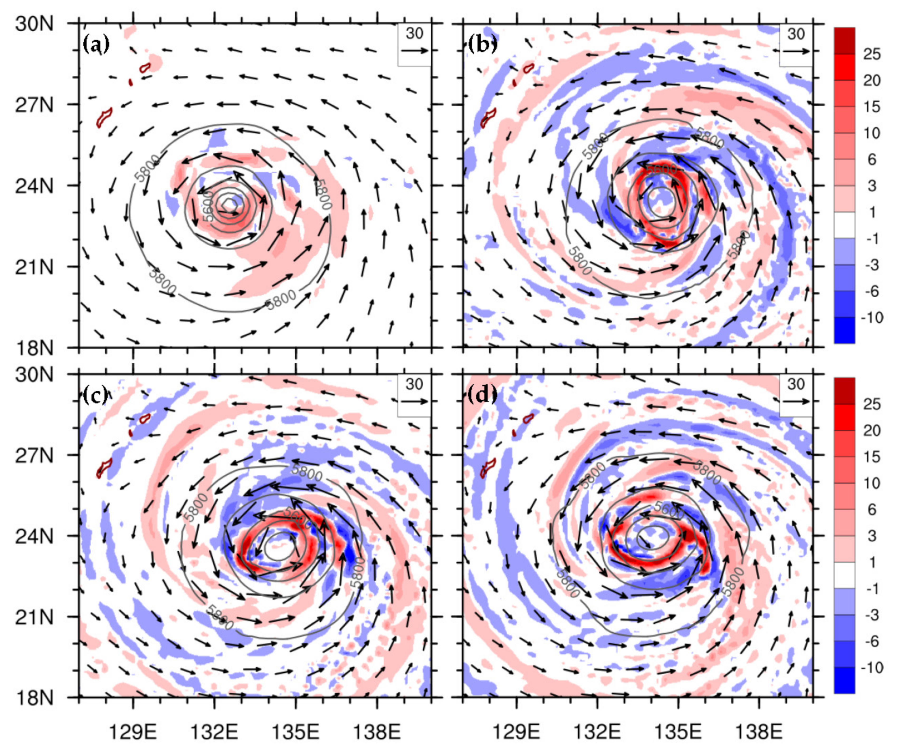
The net PV tendency budget indicates the principal direction following the major WN-1 flow direction. Thus, we used the same WN-1 PV tendency budget diagnostics as in Huang et al. [48] to quantify the contribution of each term in the PV tendency equation for the impact of GNSS RO data assimilation on typhoon translation. To diagnose the translation velocity regressed by the WN-1 flow budget in the inner vortex core, an average was computed in 1–8 km height and within a 200-km radius of the typhoon center for each term of the PV tendency budget. Figure 10 shows the net PV budget, horizontal PV advection, vertical PV advection, and differential diabatic heating terms for GTS and EPH at 48-h forecast (1200 UTC 4 September). The net WN-1 PV tendency budgets in GTS and EPH contributed northwestward translations, but EPH had a faster speed of 6.82 m s−1 than that of 2.7 m s−1 for GTS. The movements indicated by the net PV budget for EPH and GTS are consistent with the tracks in Figure 6. At this time, horizontal PV advection dominated the PV tendency budget, and it was comparable in magnitude for both GTS and EPH. Larger differences between GTS and EPH can be found in vertical PV advection and differential diabatic heating (Figure 10e–h). The vertical PV advection for EPH exhibited a westward translation which contributed to the westward component for the net PV budget. On the contrary, the vertical PV advection for GTS induced the southward vortex translation at a moving speed of about 5.5 m s−1 that largely offsets the induced northward component from horizontal PV advection. For GTS, the stronger convection at the eastern flank of the vortex in Figure 7 facilitated the southeastward translation induced by the positive upward PV advection. Some contributions may be induced by differential diabatic heating, in particular, for EPH, which showed a southward translation as 2.98 m s−1 (Figure 10g). For GTS, the contribution of differential diabatic heating was minimal (Figure 10h). Thus, GTS had a slower typhoon movement corresponding to the effect of vertical PV advection. The westward typhoon translation mainly induced by the vertical PV advection agrees with the environmental WN-1 flow, which is beneficial for the faster movement for EPH than GTS. The vertical PV advection also played an important role in the PV tendency budget at 72 h, but with opposite translations for GTS and EPH (figures not shown).
4. Sensitivity Experiments and Another Typhoon Case
4.1. Different Physical Schemes, Initial Times, and RO Observations
Model simulations may be affected by various factors, e.g., ingested observations and performed strategies of the data assimilation, physical parameterizations in the numerical model, different initial times, etc. In this study, we conducted sensitivity experiments for physics schemes, initialization time, and the number of RO observations to understand their influences on typhoon forecasts.
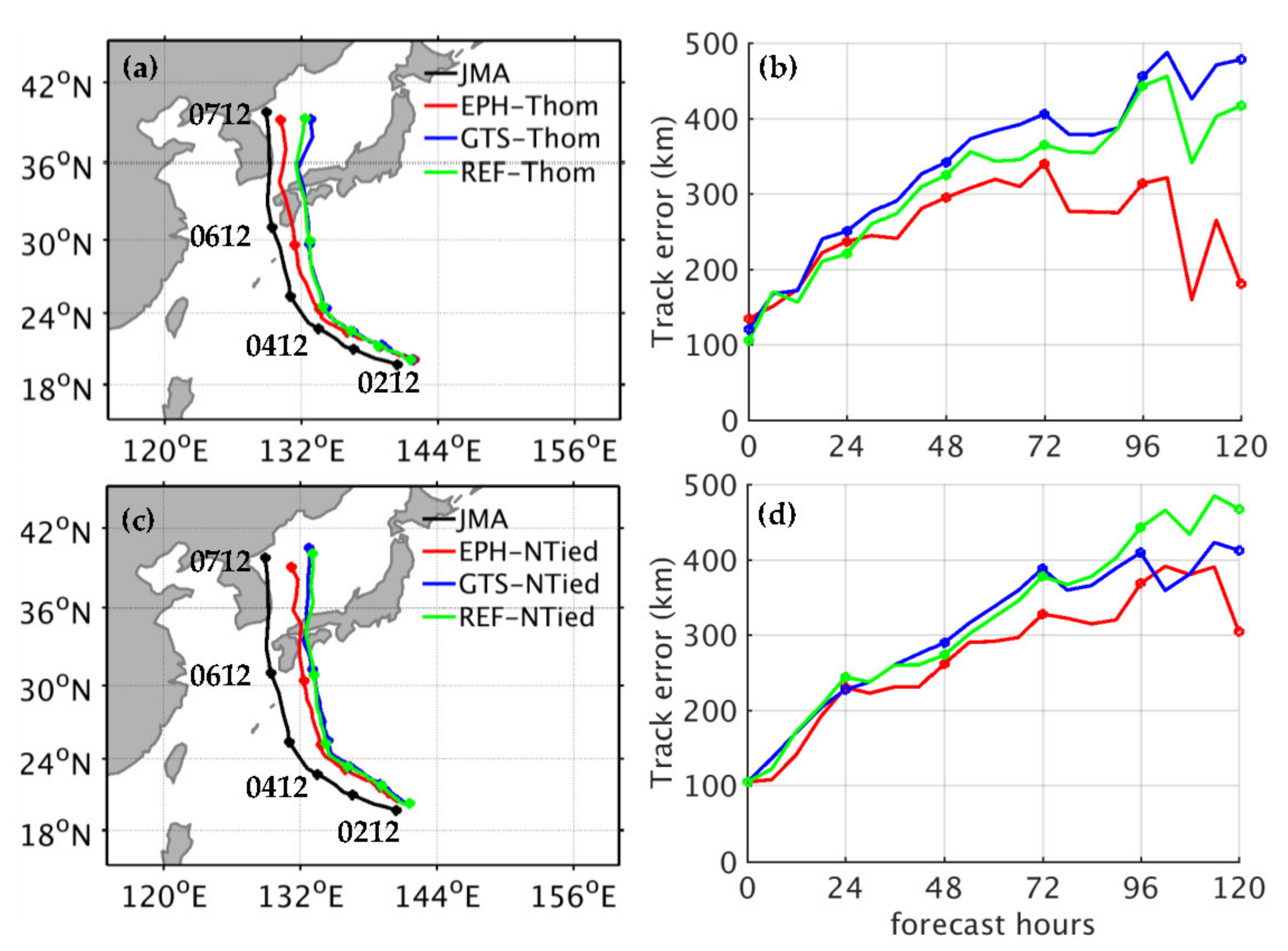
For the forecast sensitivity to physical parameterization, both microphysics and cumulus parameterization schemes are changed for both DA cycling and the WRF model integration. The replaced schemes are the Thomson scheme for the microphysics parameterization [49] and the New Tiedtke scheme for the cumulus parameterization [50]. Figure 11 shows the simulated tracks and their errors with time. With the two physics schemes, all the simulated tracks showed larger errors with an eastward deviation than those without the changes (Figure 6). For example, the track errors (Figure 11b,d) increased with time for all three experiments and were larger than the control one after the 12-h forecast (Figure 6c). Using the Thomson microphysics scheme, EPH predicted a better, more westward track than REF and GTS, with a maximum error of about 350 km at 72 h (Figure 11b). At the end of the simulation (120 h), the track was improved by more than 250 km for EPH and by only about 50 km for REF. With the New Tiedtke cumulus scheme, the simulated tracks showed similar patterns compared to those using the Thomson microphysics scheme. Clearly, EPH outperformed GTS and REF for this sensitivity test at almost all forecast time (Figure 11d). For REF, the RO data increased the track error by 50 km at 120 h compared to GTS (with no RO data assimilation).
Another sensitivity experiment used the same settings of the control run for GTS, REF, and EPH, but starting the DA 12 h earlier, i.e., performing 1-day cycling DA during 0000 UTC 1–2 September and then 5-day forecasts from 0000 UTC 2 to 7 September. The simulated tracks shown in Figure 12 were close to each other, and the track error for EPH at the initial forecast (0000 UTC 2 September) was largely reduced to 50 km (Figure 12b). Generally, the three simulated tracks were close to those of their control run (Figure 6). From Figure 12b, EPH clearly had the best performance at later stages, while GTS and REF gave nearly indistinguishable tracks throughout the simulation.
As mentioned in Section 2, the GNSS RO data came from several satellite missions in this study and were mostly contributed by FS7/C2. For the sensitivity test on RO data amounts, EPH-FS7 used the same setting as the control run, EPH, but discarded the RO soundings except for the FS7/C2 data in the data assimilation. Figure 13 shows the simulation results of EPH and EPH-FS7 for comparison. The forecasts of typhoon track and intensity were rather similar for both experiments, but their differences can be found in the typhoon moving speed that reflects the larger track errors for EPH with FS7/C2 only (Figure 13b). The track forecast was still improved after 72 h for EPH-FS7, but not as much as that for EPH (with the full RO data set). After 72 h, the performance of EPH-F7 was better than GTS (Figure 6 and Figure 13). The RO data from FS7/C2 may give comparable positive impacts when comparing this figure and Figure 6.
4.2. Typhoon Hagupit (2020)
For illustrating the impact of RO data on typhoon prediction, we conducted numerical experiments for another case, Typhoon Hagupit (2020). Typhoon Hagupit had a long life and went through several continents. First, it passed through the northern Taiwan island and then made landfall in eastern China; in the meantime, the storm rapidly developed with minimum mean-sea-level pressure (MSLP) of 975 hPa. Then the typhoon vortex turned northeastward toward Korea and Japan and brought heavy rainfall over there.
Two different initial times were conducted for WRF simulations. The initial times started at 0000 UTC and 1200 UTC on 2 August 2020, and both had a prior 1-day DA cyclin process. Figure 14 shows the simulated track and intensity and their errors with time. At an earlier initial time (0000 UTC 2 August), all the simulated tracks were close to the best track with track errors of 100–150 km before 48-h forecasts (Figure 14c). After making landfall in China, the typhoon took a more westward deflection for EPH than the other experiments but moved at slower speeds at later stages when turning eastward and offshore. These more consistent moving speeds resulted in smaller track errors after about 84 h for EPH (Figure 14a,c). The other two experiments, GTS and REF, showed faster movements than the best track after 5 August 2020. The difference in the track error between GTS and EPH exceeded 400 km at the 96-h forecast (Figure 14c). For the three DA experiments with the initial time of 1200 UTC 2 August, their tracks were less distinguishable and could be better identified after 1200 UTC 5 August. GTS predicted a southward deviation with the best track (Figure 14b), which was similar to that with the initial time 12 h earlier (Figure 14a). On the contrary, tracks for both REF and EPH closely followed the best track at later stages (Figure 14b). The simulated typhoon intensity followed the trend of the best track intensity quite well, with a reasonably captured turning point of decay near 36 h (Figure 14e) and 24 h (Figure 14f) for both EPH and REF. Although the RO impacts from the simulated results were mixed at times for Typhoon Hagupit, the GNSS RO data assimilation, particularly with the nonlocal operator (EPH), not only gave positive impacts on track forecast at later stages but also on intensity forecast at earlier stages.
5. Conclusions
FS7/C2 satellites are operating and daily provide more than 5000 thousand RO soundings over the tropical and subtropical regions, most of which have deeper penetration close to the surface with useful moisture and temperature retrievals for model analysis. In this study, we investigated the RO data impact on the prediction of Typhoon Haishen (2020) by utilizing an advanced hybrid WRFDA to assimilate RO data. Both local and nonlocal operators were available for assimilating RO retrieved refractivity, where the latter, also called excess phase operator, took into account the integrated effects of the refractivity along a GNSS ray path. The experiments using the local and nonlocal operators for RO data assimilation, denoted by REF and EPH, respectively, were conducted for comparison with the simulation without the RO data assimilation (denoted by GTS). It is the first time the impact of recently more plentiful RO data with the nonlocal operator and a hybrid system of WRFDA has been investigated. The three experiments, GTS, REF, and EPH were conducted for one-day DA with 6-h cycling and then for 5-day WRF forecasts. After DA cycling, both REF and EPH in general showed similar patterns of increments at 500 and 850 hPa, but EPH exhibited warmer temperature and more moisture around Typhoon Haishen and its upstream region than REF and GTS.
After 1-day data assimilation, the position error of the typhoon center was improved by 15.7 km for EPH in better agreement with the best track when compared to GTS. For the simulated 5-day tracks, EPH had the best performance with a mean track error of 126.5 km and a minimum error of fewer than 50 km. Compared to GTS and REF, the mean error of 5-day track prediction for EPH was reduced by about 50 km and 25 km, respectively. All three experiments captured well the intensity evolution of the observed typhoon. However, the typhoon convection was better simulated for EPH than GTS and REF. Forecast verification against the NCEP analysis for EPH also showed improvement in temperature, moisture, and wind fields at the lower troposphere. Diagnostics of PV tendency budget indicated that the translational direction of the typhoon induced by the net PV budget was consistent with the best track for EPH and GTS, but the latter had larger track errors due to the associated slower movement resulting from a larger southward component induced by vertical PV advection. On the contrary, a westward translation was induced by vertical PV advection for EPH in association with the dominant northward translation from horizontal PV advection, thus jointly producing a northwestward movement in more consistency with the best track.
In this study, sensitivity experiments for different physics schemes (cloud schemes and cumulus parameterizations), initial times, and RO data from FS7/C2 only were conducted. The physics sensitivity experiments for GTS, REF, and EPH showed larger track errors and more eastward deviations than their control runs (without changing the physics schemes). EPH still provided the best performance with significant reductions in track errors throughout the forecast. The EPH outperformance was also found for the forecast valid at an earlier initial time. FS7/C2 data contributed more than 75% of the total GNSS RO soundings during the DA period. The RO data assimilation with FS7/C2 only showed slightly larger track errors than the control run for EPH, but still gave a significant improvement on track forecast compared to that (GTS) without the RO data assimilation.
Positive impacts of RO data were also illustrated on the forecast of Typhoon Hagupit (2020) with the same experimental designs for GTS, REF, and EPH. Similarly, EPH also gave the smallest track errors at later stages. The RO data assimilation for EPH resulted in the best track forecast at later stages when Hagupit took a recurved track to move offshore from eastern China. For both RO assimilation experiments, their typhoon intensity may better follow the best track intensity than GTS.
The impacts of GNSS RO data, contributed mostly from FS7/C2, on typhoon predictions were investigated by using a hybrid DA system in this study. The hybrid system may provide more consistent flow-dependent background errors for improving the data impact in cycling assimilation. The current RO observation errors are defaults of WRFDA, which might not be optimal in the lower troposphere for the FS7 RO data. Positive RO impacts on track prediction were illustrated only for two typhoons over the WNP. We plan to investigate more typhoon cases to further demonstrate the value of RO data with updated observation errors.
Author Contributions
Conceptualization, C.-Y.H. and S.-Y.C.; Methodology, S.-Y.C.; Validation, Analysis, and Investigation, C.-Y.H., S.-Y.C. and T.-C.N.; Writing–Original Draft Preparation, S.-Y.C. and T.-C.N.; Writing–Review & Editing, S.-Y.C., C.-Y.H. and T.-C.N.; Supervision, C.-Y.H.; Project Administration, C.-Y.H. and S.-Y.C. All authors have read and agreed to the published version of the manuscript.
Funding
This study was supported by the Ministry of Science and Technology (MOST) (grant No. MOST-110-2111-M-008-014) and the National Space Organization (NSPO) (grant No. NSPO-S-109138) in Taiwan.
Institutional Review Board Statement
Not applicable.
Informed Consent Statement
Not applicable.
Data Availability Statement
The best track data are obtained from the JMA, and the model forecasts are available from the workstation of the typhoon laboratory at the Department of Atmospheric Sciences, National Central University, in contact with C.-Y. Huang and S.-Y. Chen.
Acknowledgments
The authors thank the National Center for High-Performance Computing (NCHC) for providing computational and storage resources, and Taiwan Analysis Center for COSMIC (TACC) and Central Weather Bureau (CWB) for providing observations.
Conflicts of Interest
The authors declare no conflict of interest.
References
- Ho, S.-P.; Anthes, R.A.; Ao, C.O.; Healy, S.; Horanyi, A.; Hunt, D.; Mannucci, A.J.; Pedatella, N.; Randel, W.J.; Simmons, A. The COSMIC/FORMOSAT-3 radio occultation mission after 12 years: Accomplishments, remaining challenges, and potential impacts of COSMIC-2. Bull. Am. Meteorol. Soc. 2020, 101, E1107–E1136. [Google Scholar] [CrossRef] [Green Version]
- Healy, S.; Thépaut, J.N. Assimilation experiments with CHAMP GPS radio occultation measurements. Q. J. R. Meteorol. Soc. 2006, 132, 605–623. [Google Scholar] [CrossRef]
- Cucurull, L.; Derber, J.; Treadon, R.; Purser, R. Assimilation of global positioning system radio occultation observations into NCEP’s global data assimilation system. Mon. Weather Rev. 2007, 135, 3174–3193. [Google Scholar] [CrossRef] [Green Version]
- Aparicio, J.M.; Deblonde, G. Impact of the assimilation of CHAMP refractivity profiles on Environment Canada global forecasts. Mon. Weather Rev. 2008, 136, 257–275. [Google Scholar] [CrossRef]
- Poli, P.; Beyerle, G.; Schmidt, T.; Wickert, J. Assimilation of GPS radio occultation measurements at Météo-France. In Proceedings of the GRAS SAF Workshop on Applications of GPSRO Measurements, ECMWF, Reading, UK, 16–18 June 2008; pp. 16–18. [Google Scholar]
- Rennie, M. The impact of GPS radio occultation assimilation at the Met Office. Q. J. R. Meteorol. Soc. 2010, 136, 116–131. [Google Scholar] [CrossRef]
- Schreiner, W.S.; Weiss, J.; Anthes, R.A.; Braun, J.; Chu, V.; Fong, J.; Hunt, D.; Kuo, Y.H.; Meehan, T.; Serafino, W. COSMIC-2 radio occultation constellation: First results. Geophys. Res. Lett. 2020, 47, e2019GL086841. [Google Scholar] [CrossRef]
- Ho, S.-P.; Zhou, X.; Shao, X.; Zhang, B.; Adhikari, L.; Kireev, S.; He, Y.; Yoe, J.G.; Xia-Serafino, W.; Lynch, E. Initial assessment of the COSMIC-2/FORMOSAT-7 neutral atmosphere data quality in NESDIS/STAR using in situ and satellite data. Remote Sens. 2020, 12, 4099. [Google Scholar] [CrossRef]
- Chen, S.-Y.; Liu, C.-Y.; Huang, C.-Y.; Hsu, S.-C.; Li, H.-W.; Lin, P.-H.; Cheng, J.-P.; Huang, C.-Y. An Analysis Study of FORMOSAT-7/COSMIC-2 Radio Occultation Data in the Troposphere. Remote Sens. 2021, 13, 717. [Google Scholar] [CrossRef]
- Anthes, R.; Sjoberg, J.; Rieckh, T.; Wee, T.-K.; Zeng, Z. COSMIC-2 radio occultation temperature, specific, humidity, and precipitable water in Hurricane Dorian (2019). Terr. Atmos. Ocean. Sci. 2021. [Google Scholar] [CrossRef]
- Cucurull, L.; Casey, S. Improved impacts in observing system simulation experiments of radio occultation observations as a result of model and data assimilation changes. Mon. Weather Rev. 2021, 149, 207–220. [Google Scholar] [CrossRef]
- Healy, S. ECMWF starts assimilating COSMIC-2 data. ECMWF Newsl. 2020, 163, 5–6. [Google Scholar]
- Shao, H.; Bathmann, K.; Zhang, H.; Huang, Z.; Cucurull, L.; Vandenberghe, F.; Treadon, R.; Kleist, D.; Yoe, J. COSMIC-2 NWP assessment and implementation at JCSDA and NCEP. In Proceedings of the 5th International Conference on GPS Radio and Occultation, Taipei, Taiwan, 21–23 October 2020. [Google Scholar]
- Lien, G.-Y.; Lin, C.-H.; Huang, Z.-M.; Teng, W.-H.; Chen, J.-H.; Lin, C.-C.; Ho, H.-H.; Huang, J.-Y.; Hong, J.-S.; Cheng, C.-P. Assimilation Impact of Early FORMOSAT-7/COSMIC-2 GNSS Radio Occultation Data with Taiwan’s CWB Global Forecast System. Mon. Weather Rev. 2021, 149, 2171–2191. [Google Scholar]
- Bonafoni, S.; Biondi, R.; Brenot, H.; Anthes, R. Radio occultation and ground-based GNSS products for observing, understanding and predicting extreme events: A review. Atmos. Res. 2019, 230, 104624. [Google Scholar] [CrossRef]
- Chen, S.-Y.; Kuo, Y.-H.; Huang, C.-Y. The impact of GPS RO data on the prediction of tropical cyclogenesis using a nonlocal observation operator: An initial assessment. Mon. Weather Rev. 2020, 148, 2701–2717. [Google Scholar] [CrossRef]
- Chen, S.-Y.; Huang, C.-Y.; Kuo, Y.-H.; Guo, Y.-R.; Sokolovskiy, S. Assimilation of GPS refractivity from FORMOSAT-3/COSMIC using a nonlocal operator with WRF 3DVAR and its impact on the prediction of a typhoon event. Terr. Atmos. Ocean. Sci. 2009, 20, 133–154. [Google Scholar] [CrossRef] [Green Version]
- Kueh, M.-T.; Huang, C.-Y.; Chen, S.-Y.; Chen, S.-H.; Wang, C.-J. Impact of GPS Radio Occultation Refractivity Soundings on a Simulation of Typhoon Bilis (2006) upon Landfall. Terr. Atmos. Ocean. Sci. 2009, 20, 115–131. [Google Scholar] [CrossRef] [Green Version]
- Chen, Y.-C.; Hsieh, M.-E.; Hsiao, L.-F.; Kuo, Y.-H.; Yang, M.-J.; Huang, C.-Y.; Lee, C.-S. Systematic evaluation of the impacts of GPSRO data on the prediction of typhoons over the northwestern Pacific in 2008–2010. Atmos. Meas. Tech. 2015, 8, 2531–2542. [Google Scholar] [CrossRef] [Green Version]
- Hamill, T.M.; Snyder, C. A hybrid ensemble Kalman filter–3D variational analysis scheme. Mon. Weather Rev. 2000, 128, 2905–2919. [Google Scholar] [CrossRef]
- Wang, X.; Barker, D.M.; Snyder, C.; Hamill, T.M. A hybrid ETKF–3DVAR data assimilation scheme for the WRF model. Part II: Real observation experiments. Mon. Weather Rev. 2008, 136, 5132–5147. [Google Scholar] [CrossRef] [Green Version]
- Bannister, R. A review of operational methods of variational and ensemble-variational data assimilation. Q. J. R. Meteorol. Soc. 2017, 143, 607–633. [Google Scholar] [CrossRef] [Green Version]
- Schwartz, C.S.; Liu, Z.; Huang, X.-Y.; Kuo, Y.-H.; Fong, C.-T. Comparing limited-area 3DVAR and hybrid variational-ensemble data assimilation methods for typhoon track forecasts: Sensitivity to outer loops and vortex relocation. Mon. Weather Rev. 2013, 141, 4350–4372. [Google Scholar] [CrossRef]
- Skamarock, W.C.; Klemp, J.B.; Dudhia, J.; Gill, D.O.; Barker, D.M.; Wang, W.; Powers, J.G. A description of the Advanced Research WRF version 3. In NCAR Technical Note-475+ STR; National Center for Atmospheric Research: Boulder, CO, USA, 2008. [Google Scholar]
- Research Data Archive at the National Center for Atmospheric Research, Computational and Information Systems Laboratory. Available online: https://rda.ucar.edu/datasets/ds083.3/ (accessed on 14 September 2021).
- Tao, W.-K.; Simpson, J.; McCumber, M. An ice-water saturation adjustment. Mon. Weather Rev. 1989, 117, 231–235. [Google Scholar] [CrossRef] [Green Version]
- Tao, W.K.; Wu, D.; Lang, S.; Chern, J.D.; Peters-Lidard, C.; Fridlind, A.; Matsui, T. High-resolution NU-WRF simulations of a deep convective-precipitation system during MC3E: Further improvements and comparisons between Goddard microphysics schemes and observations. J. Geophys. Res. Atmos. 2016, 121, 1278–1305. [Google Scholar] [CrossRef]
- Kain, J.S. The Kain–Fritsch convective parameterization: An update. J. Appl. Meteorol. 2004, 43, 170–181. [Google Scholar] [CrossRef] [Green Version]
- Hong, S.-Y.; Noh, Y.; Dudhia, J. A new vertical diffusion package with an explicit treatment of entrainment processes. Mon. Weather Rev. 2006, 134, 2318–2341. [Google Scholar] [CrossRef] [Green Version]
- Iacono, M.J.; Delamere, J.S.; Mlawer, E.J.; Shephard, M.W.; Clough, S.A.; Collins, W.D. Radiative forcing by long-lived greenhouse gases: Calculations with the AER radiative transfer models. J. Geophys. Res. Atmos. 2008, 113, D13103. [Google Scholar] [CrossRef]
- Barker, D.; Huang, Z.-Y.; Liu, Z.; Auligné, T.; Zhang, X.; Rugg, S.; Ajjaji, R.; Bourgeoi, A.; Bray, J.; Chen, Y.; et al. The weather research and forecasting model’s community variational/ensemble data assimilation system: WRFDA. Bull. Am. Meteorol. Soc. 2012, 93, 831–843. [Google Scholar] [CrossRef] [Green Version]
- Barker, D.M.; Huang, W.; Guo, Y.-R.; Bourgeois, A.; Xiao, Q. A three-dimensional variational data assimilation system for MM5: Implementation and initial results. Mon. Weather Rev. 2004, 132, 897–914. [Google Scholar] [CrossRef] [Green Version]
- Huang, X.-Y.; Xiao, Q.; Barker, D.M.; Zhang, X.; Michalakes, J.; Huang, W.; Henderson, T.; Bray, J.; Chen, Y.; Ma, Z. Four-dimensional variational data assimilation for WRF: Formulation and preliminary results. Mon. Weather Rev. 2009, 137, 299–314. [Google Scholar] [CrossRef] [Green Version]
- Bishop, C.H.; Etherton, B.J.; Majumdar, S.J. Adaptive sampling with the ensemble transform Kalman filter. Part I: Theoretical aspects. Mon. Weather Rev. 2001, 129, 420–436. [Google Scholar] [CrossRef]
- Wang, X.; Bishop, C.H. A comparison of breeding and ensemble transform Kalman filter ensemble forecast schemes. J. Atmos. Sci. 2003, 60, 1140–1158. [Google Scholar] [CrossRef]
- Wang, X.; Barker, D.M.; Snyder, C.; Hamill, T.M. A hybrid ETKF–3DVAR data assimilation scheme for the WRF model. Part I: Observing system simulation experiment. Mon. Weather Rev. 2008, 136, 5116–5131. [Google Scholar] [CrossRef] [Green Version]
- Hamill, T.M.; Whitaker, J.S.; Kleist, D.T.; Fiorino, M.; Benjamin, S.G. Predictions of 2010’s tropical cyclones using the GFS and ensemble-based data assimilation methods. Mon. Weather Rev. 2011, 139, 3243–3247. [Google Scholar] [CrossRef] [Green Version]
- Kleist, D.T. An Evaluation of Hybrid Variational-Ensemble Data Assimilation for the NCEP GFS; University of Maryland: College Park, MD, USA, 2012. [Google Scholar]
- National Center for Atmospheric Research, Mesoscale & Microscale Meteorology Laboratory. Available online: https://www.mmm.ucar.edu/weather-research-and-forecasting-model (accessed on 14 September 2021).
- Yang, S.-C.; Chen, S.-H.; Chen, S.-Y.; Huang, C.-Y.; Chen, C.-S. Evaluating the impact of the COSMIC RO bending angle data on predicting the heavy precipitation episode on 16 June 2008 during SoWMEX-IOP8. Mon. Weather Rev. 2014, 142, 4139–4163. [Google Scholar] [CrossRef] [Green Version]
- Huang, C.-Y.; Chen, S.-Y.; Anisetty, S.P.R.; Yang, S.-C.; Hsiao, L.-F. An impact study of GPS radio occultation observations on frontal rainfall prediction with a local bending angle operator. Weather Forecast. 2016, 31, 129–150. [Google Scholar] [CrossRef]
- Smith, E.K.; Weintraub, S. The constants in the equation for atmospheric refractive index at radio frequencies. Proc. IRE 1953, 41, 1035–1037. [Google Scholar] [CrossRef] [Green Version]
- Sokolovskiy, S.; Kuo, Y.-H.; Wang, W. Assessing the accuracy of a linearized observation operator for assimilation of radio occultation data: Case simulations with a high-resolution weather model. Mon. Weather Rev. 2005, 133, 2200–2212. [Google Scholar] [CrossRef] [Green Version]
- Zhang, X.; Kuo, Y.-H.; Chen, S.-Y.; Huang, X.-Y.; Hsiao, L.-F. Parallelization strategies for the GPS radio occultation data assimilation with a nonlocal operator in the weather research and forecasting model. J. Atmos. Ocean. Technol. 2014, 31, 2008–2014. [Google Scholar] [CrossRef]
- Wu, L.; Wang, B. A potential vorticity tendency diagnostic approach for tropical cyclone motion. Mon. Weather Rev. 2000, 128, 1899–1911. [Google Scholar] [CrossRef] [Green Version]
- Chan, J.C.; Ko, F.M.; Lei, Y.M. Relationship between potential vorticity tendency and tropical cyclone motion. J. Atmos. Sci. 2002, 59, 1317–1336. [Google Scholar] [CrossRef]
- Li, D.Y.; Huang, C.Y. The influences of orography and ocean on track of Typhoon Megi (2016) past Taiwan as identified by HWRF. J. Geophys. Res. Atmos. 2018, 123, 11492–411517. [Google Scholar] [CrossRef]
- Huang, C.-Y.; Huang, C.-H.; Skamarock, W.C. Track deflection of Typhoon Nesat (2017) as realized by multiresolution simulations of a global model. Mon. Weather Rev. 2019, 147, 1593–1613. [Google Scholar] [CrossRef] [Green Version]
- Thompson, G.; Field, P.R.; Rasmussen, R.M.; Hall, W.D. Explicit forecasts of winter precipitation using an improved bulk microphysics scheme. Part II: Implementation of a new snow parameterization. Mon. Weather Rev. 2008, 136, 5095–5115. [Google Scholar] [CrossRef]
- Zhang, C.; Wang, Y. Projected future changes of tropical cyclone activity over the western North and South Pacific in a 20-km-mesh regional climate model. J. Clim. 2017, 30, 5923–5941. [Google Scholar] [CrossRef]
Figure 1.
The model domains with 15-km and 3-km resolutions for the outermost domain (blue) and the inner domain (red), respectively. The best track of Typhoon Haishen (2020) from JMA is indicated by the black line with plus symbols at a 6-h interval. The green dashed box indicates the region for forecast verification.

Figure 2.
(a) The flowchart of the hybrid WRFDA data assimilation system. The ETKF employs 32 members with the outermost domain to provide the background error covariance. Both ETKF and 3DEnVar were conducted for the domain with the 15-km resolution, and the final analysis was adopted for the two domains of 15-km and 3-km resolutions. (b) The experimental design. Each simulation was carried out by 1-day cycling data assimilation with a 6-h cycling interval and then forecast for 5 days.

Figure 3.
(a) The horizontal distribution of GNSS RO data during the 1-day DA period. There was a total of 959 RO soundings in the outermost domain, including 724 data from FORMOSAT-7/COSMIC2 (red), 222 from MetOp (blue), 7 from KOMPSAT-5 (green), and 6 from PAZ (brown). (b) The vertical variation of the amounts of accumulated RO soundings at each DA cycling, e.g., 01_12 indicates the DA time at 1200 UTC 01 September 2020 (the first DA cycle), and 02_12 is for the DA time at the final DA cycle.

Figure 4.
(a) Difference in temperature (shaded colors; K) at 500 hPa between REF and GTS after the first DA cycle at 1200 UTC 1 September. (b) as in (a), but between EPH and GTS. (c,d) as in (a,b), respectively, but at 850 hPa. (e,f) as in (c,d), respectively, but for water vapor mixing ratio (shaded colors; g kg−1). The dot points indicate the locations of GNSS RO, and the circled cross symbol indicates the center location of Typhoon Haishen at 1200 UTC 1 September reported by JMA.

Figure 5.
As in Figure 4, but for the time-averaged differences.
Figure 5.
As in Figure 4, but for the time-averaged differences.

Figure 6.
(a) The best track (black) from JMA of Typhoon Haishen (2020) and WRF simulated tracks for GTS (blue), REF (green), and EPH (red) during 1200 UTC 2–7 September 2020. (b) Same as in (a), but for the zoomed region indicated by the black-dashed box in (a). (c) The track errors of Typhoon Haishen (2020) for GTS (blue), REF (green), and EPH (red) during 1200 UTC 2–7 September 2020. (d) as in (c), but are the maximum wind speed (Vmax, in m s−1) for simulated typhoon intensities and best track (in black). Circle symbols indicate the outputs every 24 h.

Figure 7.
(a) Infrared satellite image from Himawari-8, and the simulated outgoing longwave radiation flux (W m−2) at 1800 UTC 4 September 2020 (54-h forecast) for (b) GTS, (c) REF, and (d) EPH.
Figure 7.
(a) Infrared satellite image from Himawari-8, and the simulated outgoing longwave radiation flux (W m−2) at 1800 UTC 4 September 2020 (54-h forecast) for (b) GTS, (c) REF, and (d) EPH.

Figure 8.
Simulated horizontal wind (wind vectors; m s−1), geopotential height (contour lines; gpm), and vertical velocity (shaped colors; m s−1) at 500 hPa for (a) NCEP, (b) GTS, (c) REF, and (d) EPH at 54-h forecast (i.e., 1800 UTC 4 September 2020).
Figure 8.
Simulated horizontal wind (wind vectors; m s−1), geopotential height (contour lines; gpm), and vertical velocity (shaped colors; m s−1) at 500 hPa for (a) NCEP, (b) GTS, (c) REF, and (d) EPH at 54-h forecast (i.e., 1800 UTC 4 September 2020).

Figure 9.
The RMSE of the model forecast for the experiments EPH (red), GTS (blue), and REF (green) verified against the NCEP analysis over 10–30° N, and 130–160° E, for (a) temperature (K), (b) water vapor mixing ratio (g kg−1), (c) east–west wind component (u), and (d) north–south wind component (v), at 48-h forecast (1200 UTC 4 September 2020).

Figure 10.
The horizontal wind and wavenumber-1 (WN-1) PV tendency budget (shaded colors, 10−5 PVU s−1) averaged in 1–8 km height at 1200 UTC 4 September 2020 for EPH for (a) net PV budget, (c) horizontal PV advection, (e) vertical PV advection, and (g) differential diabatic heating. (b,d,f,h) as in (a,c,e,g), respectively, but for GTS. The bold reference wind vector (in m s−1) at the vortex center indicates the induced net translation velocity, and a reference wind vector (m s−1) is given in the upper right of each panel for the wind speed.

Figure 11.
(a) Simulated tracks of Haishen for EPH-Thom (red line), GTS-Thom (blue line), and REF-Thom (green line) experiments and the best tracks of JMA (black line). The Thompson microphysics scheme was used in the three experiments. (b) as in (a) but for track error. (c) as in (a) but using the New Tiedtke cumulus parameterization. (d) as in (c) but for track error. Circle symbols in (a,b) mark the typhoon centers every 24 h.

Figure 12.
(a) Simulated tracks of Haishen for 090200-EPH (red line), 090200-GTS (blue line), and 090200-REF (green line) experiments and the best tracks of JMA (black line). The simulated time was from 0000 UTC 2 September to 0000 UTC 7 September 2020. (b) as in (a) but for track error. Circle symbols mark the typhoon centers every 24 h.

Figure 13.
(a) Simulated tracks for EPH (red) and EPH-F7 (blue) and the best tracks from JMA (black). (b–d) as in (a), but for the (b) track errors (in km), (c) MSLP (hPa), and (d) maximum wind speed (Vmax in m s−1), respectively. Circle symbols mark the typhoon centers every 24 h.
Figure 13.
(a) Simulated tracks for EPH (red) and EPH-F7 (blue) and the best tracks from JMA (black). (b–d) as in (a), but for the (b) track errors (in km), (c) MSLP (hPa), and (d) maximum wind speed (Vmax in m s−1), respectively. Circle symbols mark the typhoon centers every 24 h.

Figure 14.
(a) Simulated tracks of Hagupit for experiments, GTS (blue), REF (green), and EPH (red), and the best tracks from JMA (black). The simulated time was from 0000 UTC 2–7 August 2020. (b) as in (a) but for the simulated time from 1200 UTC 2–7 August 2020. (c,d) as in (a,b), respectively, but for track error (km). (e,f) as in (a,b), respectively, but for MSLP (hPa). Circle symbols in (a,b) mark the typhoon centers every 24 h.


Table 1.
Experimental design for Typhoon Haishen (2020).
| Name | Description |
|---|---|
| GTS (CTL) | Control assimilation with the convectional data and satellite retrieved wind |
| REF | Same as GTS, but assimilating additional GNSS RO data with the local REFractivity operator |
| EPH | Same as REF, but using the nonlocal pseudo–Excess PHase operator |
Publisher’s Note: MDPI stays neutral with regard to jurisdictional claims in published maps and institutional affiliations. |
© 2021 by the authors. Licensee MDPI, Basel, Switzerland. This article is an open access article distributed under the terms and conditions of the Creative Commons Attribution (CC BY) license (https://creativecommons.org/licenses/by/4.0/).
Share and Cite
MDPI and ACS Style
Chen, S.-Y.; Nguyen, T.-C.; Huang, C.-Y. Impact of Radio Occultation Data on the Prediction of Typhoon Haishen (2020) with WRFDA Hybrid Assimilation. Atmosphere 2021, 12, 1397. https://0-doi-org.brum.beds.ac.uk/10.3390/atmos12111397
AMA Style
Chen S-Y, Nguyen T-C, Huang C-Y. Impact of Radio Occultation Data on the Prediction of Typhoon Haishen (2020) with WRFDA Hybrid Assimilation. Atmosphere. 2021; 12(11):1397. https://0-doi-org.brum.beds.ac.uk/10.3390/atmos12111397
Chicago/Turabian StyleChen, Shu-Ya, Thi-Chinh Nguyen, and Ching-Yuang Huang. 2021. "Impact of Radio Occultation Data on the Prediction of Typhoon Haishen (2020) with WRFDA Hybrid Assimilation" Atmosphere 12, no. 11: 1397. https://0-doi-org.brum.beds.ac.uk/10.3390/atmos12111397
Note that from the first issue of 2016, this journal uses article numbers instead of page numbers. See further details here.