Article

Bottom–Up Inventory of Residential Combustion Emissions in Poland for National Air Quality Modelling: Current Status and Perspectives

Institute of Environmental Protection–National Research Institute, Krucza 5/11D, 00-548 Warsaw, Poland
*
Author to whom correspondence should be addressed.
Submission received: 30 September 2021 / Revised: 26 October 2021 / Accepted: 28 October 2021 / Published: 4 November 2021
(This article belongs to the Special Issue Air Quality in Poland)

Abstract

:
For many years, the Polish air quality modelling system was decentralized, which significantly hampered the appropriate development of methodologies, evaluations, and comparisons of modelling results. The major contributor to air pollution in Poland is the residential combustion sector. This paper demonstrates a novel methodology for residential emission estimation utilized for national air quality modelling and assessment. Our data were compared with EMEP and CAMS inventories, and despite some inequalities in country totals, spatial patterns were similar. We discuss the shortcomings of the presented method and draw conclusions for future improvements.

1. Introduction

One of the best sources of air quality (AQ) information is a network of atmospheric measurements sites. In order to provide comprehensive AQ assessment, data collected by such observational stations should be supplemented with AQ modelling, which can provide full spatial coverage over vast areas. AQ modelling is dependent on the emission input data, models used, and methodologies applied. AQ models are frequently evaluated [1,2,3,4,5], but some studies have identified emission inventories as one of the primary sources of uncertainty in the modelling chain [6,7]. This is connected with the fact that the estimation of atmospheric pollution emissions is very challenging, primarily because of the lack of appropriate activity data due to several reasons. First of all, it is common in many countries that there is no centralized database that can provide spatially resolved and consistent information about fuel sales or fuel usage on a national scale. Secondly, the data are frequently trade secrets or incomplete and uncertain. Thirdly, many entities (e.g., cities or local governments) create their databases, which are, in many cases, not comparable with each other. This inevitably leads to significant discrepancies in AQ modelling results.
Pollutant emissions are connected with specific human activities, some of which are commonly observed. For example, road traffic (similarly to agricultural production) is often monitored because of their significance for economy. Although the main goal of collecting such data is not emission estimation, it can be easily adopted. Unfortunately, human activities (besides population) connected with residential combustion are typically not monitored directly. It is hard to connect residential combustion to a measurable output, as can be done in other economy sectors e.g. electricity is the output of the power generation sector and goods are the output of the industrial sector. Hence, it can be a source of significant uncertainties in emission inventories [8]. Moreover, various furnaces and fuels are used, and it is difficult to analyze and catalogue them or formulate emission factors. Although there are examples of comprehensive emission inventories for the residential sector based on fuel consumption [9,10], data access for emission estimation is problematic in many countries. For example, investigators in Norway use a web-crawler that uses online estate adverts in order to collect data [11]; some investigations in China employ indirect methods such as regression models for fuel consumption estimation [12]; and surveys have been utilized for data collection in Vietnam [13], China [14,15], and Lombardy (Italy) [16]. Other approaches utilize comprehensive measurement campaigns as a basis for emission inventories [17,18] or GIS-based gap-filling [19].
Poor AQ was a basis for the Court of Justice of the European Union (CJEU) sentence (from 28 February 2018) against Poland for permanent exceedances of PM10 norms (established in EU Parliament and Council Directive 2008/50/WE on 21 May 2008). Even though many activities have been undertaken to reduce emissions throughout the last two decades, AQ in Poland is still unsatisfactory. PM10, PM2.5, and B(a)P limit values are often exceeded in many parts of the country. The major source of those pollutants is residential fuel combustion for heating purposes.
Like in other countries, Poland had no comprehensive database that can provide consistent information for national AQ modelling for many years. Such data are necessary for any national air protection system to operate. Recently, much effort has been put into residential wood combustion (RWC) emission estimation [17,20,21,22,23]. In Poland, in terms of national residential combustion emission inventory, RWC is not a priority issue at the moment, since the most currently challenging issue the collection and unification of various data from diversified sources into a consistent and comprehensive database that can allow for the best possible AQ modelling results. There are still many gaps in our knowledge, e.g., access to grid heating, renewable energy sources, fuels consumption (including wood), and building insulation.
Air quality modelling in Poland was initially done by separate regional Environment Protection Inspection groups, often using different models or methodologies. In practice, tasks were performed using varying methods and materials (such as emission inventories and meteorological data). Since 2013, attempts have been made to implement centralized AQ modelling. However, tasks were assigned as short-term contracts. Moreover, the system did not have stable funding, which seriously hampered scientific development and improvement possibilities.
In the year 2019, a novel legal act was introduced that changed how the national AQ modelling system was organized. From then on, AQ modelling and the preparation of an emission database is the duty of the Institute of Environmental Protection–National Research Institute (IEP–NRI). This change allowed for the consequent development and enhancement of AQ modelling and emission inventory in one central institution. The IEP–NRI is responsible for emission estimation from all of existing sources (Central Emission Database—CED) from all sectors, namely residential, transport, industry, agriculture, natural sources, and other (such as landfills, excavation sites, and mining heaps). The inventory was created for the purpose of national AQ modelling. It is utilized as an input for the GEM-AQ model [24]. The results of modelling serve as supplements for in situ AQ monitoring, which constitutes the basis of the ChIEP (Chief Inspectorate for Environmental Protection) Air Quality Annual Assessments.
The main goal of this manuscript was to present the current methodology of residential emission estimation, discuss perspectives for development, and compare existing data with well-known inventories: EMEP and CAMS. Our methodology has clear advantages: it is a bottom–up inventory (which allows for the indirect inclusion of local databases) and was designed for individual buildings that allow for almost any AQ modelling spatial resolution.

2. Materials and Methods

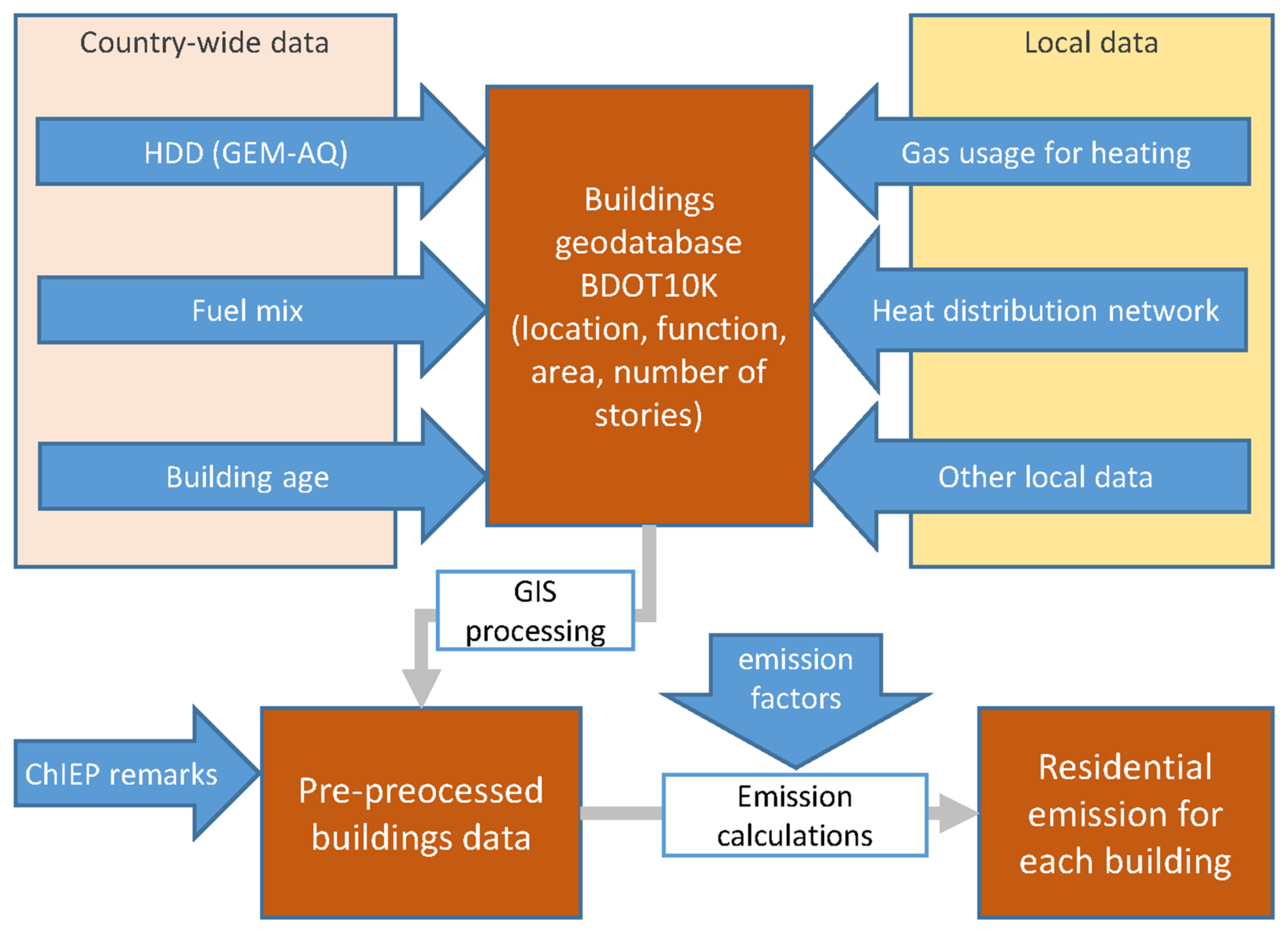
2.1. CED Emission Inventory

The CED inventory follows a bottom–up methodology. The data presented here were prepared in late 2020 and early 2021, were based on data from 2019, and were utilized in the 2020 ChIEP AQ Annual Assessment [25].
Residential emission estimation in the CED is dependent on several inputs (Table 1). The spatial resolution is not equal for all data, and some datasets do not have resolution since accurate vector geometries with spatial reference represent them. For example, heating degree days (HDD) are calculated in a grid using GEM-AQ data with a resolution of 0.025 degrees for the entire country. At the same time, the fuel mix is available not in a regular grid but as table data for each “district unit” (administrative units without uniform spatial coverage—we distinguished 3592 such units for our purposes). All of the data were assigned to buildings using their geographical location.
Since input data were taken from various sources, unification was a challenge. For example, heat distribution network data are stored in various formats following different standards in each of Poviat Centers for Geodetic and Cartographic Documentation (380 in Poland). Building a uniform database with a country-wide database required sending an official request for data access. When it was granted, the data were downloaded and processed to be included in the CED. The heat distribution network and other data served as proxies to determine which buildings have individual heat sources (and thus emit pollution) and which do not. This is a critical step in our methodology. We present a flowchart of our methodology in Figure 1.
The ChIEP evaluates the CED on a regular basis. Experts check groups or individual buildings and provide coded notes if some changes are necessary. Several building features are considered, e.g., link to heat or gas network, fuel mix, and building function. These features are included when emissions are processed for GEM-AQ model input.
The first step of emission processing is to combine all country-wide and local data for individual buildings. The second step is to calculate heat demand (HD) and to address ChIEP remarks. The last step is to calculate emissions using appropriate emission factors. For the ChIEP AQ Annual Assessment, the discharge of 8 pollutants (SOx, NOx, PM10, PM2.5, TSP, CO, NMVOC, and B(a)P) is estimated.
Below, we present currently utilized emission factors (Table 2) and annual country totals (Table 3). The annual emission discharge per cell (spatial pattern) values of SOx, NOx, and PM10 are presented in Figure 2.
Since emissions are calculated via simple multiplication (Factor x HD), slight changes in the values of factors strongly impact the resulting emission discharge. Therefore, any changes in emission factors must be applied with extreme care.
The CED is regularly improved. New heat distribution networks are included once they are obtained from data providers. Fuel mixes are evaluated with the help of the ChIEP and by using local emission inventories, which are systematically analyzed and included in the CED. Currently, the main focus of residential sector improvement is on aspects such as new data inclusion, cooperation with the ChIEP, and fuel mixes. For more information, please refer to the discussion section.

2.2. EMEP and CAMS-REG Emission Inventories
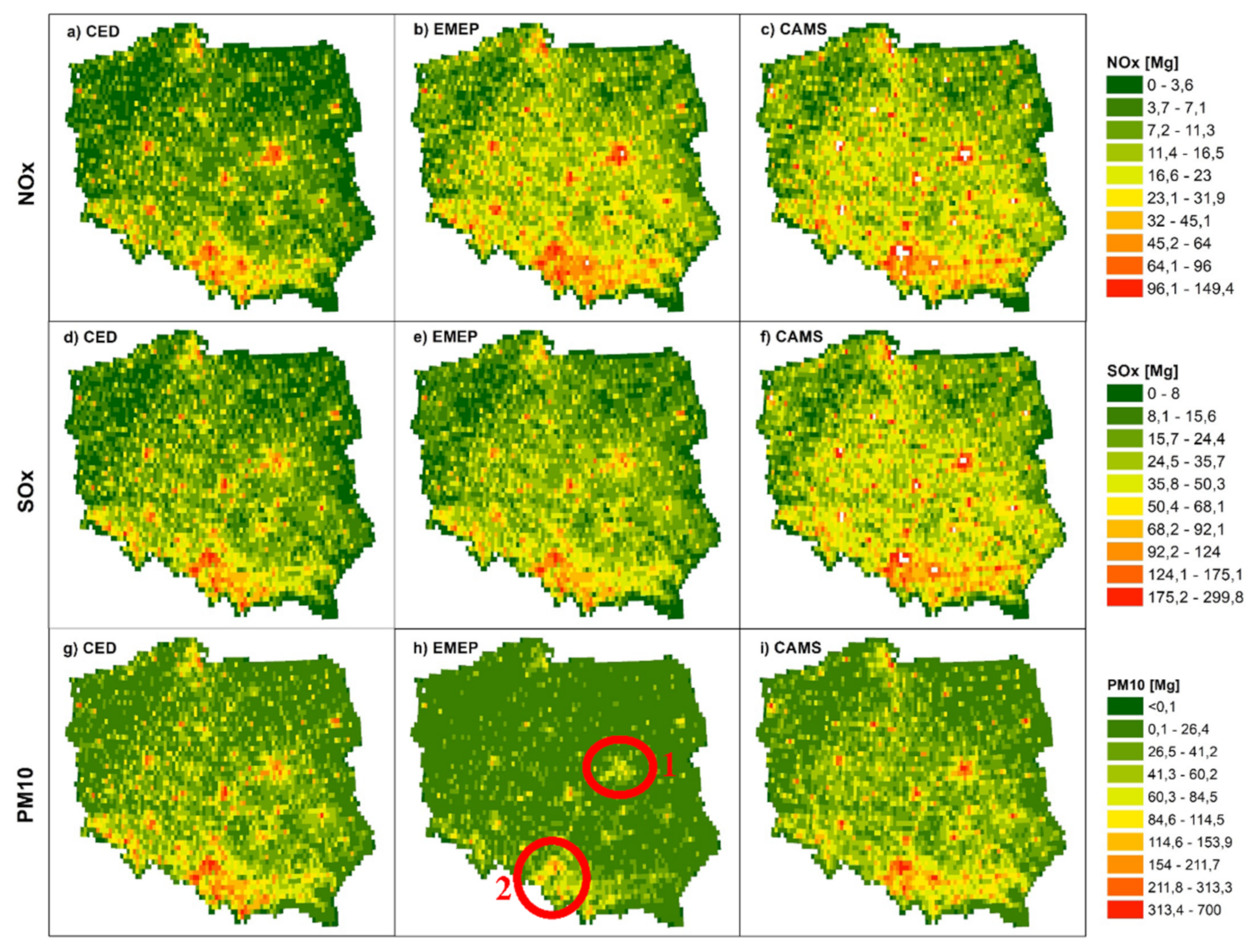
The EMEP (European Monitoring and Evaluation Programme) is a scientifically based and policy-driven framework under the Convention on Long-Range Transboundary Air Pollution (CLRTAP). Poland, among other countries, is obliged to report national totals of pollutants. The reported data are spatially disaggregated into regular grids [26,27].
The Copernicus Atmosphere Monitoring Service (CAMS) is one of six services that form Copernicus, the European Union’s Earth observation framework. Copernicus offers information services based on satellite Earth observation (i.e., Sentinel), in situ data, and modelling. The CAMS is focused on Europe, but it also offers global products. The core of the CAMS-REG-v4 inventory are the country totals reported to the EMEP, which are re-gridded following the methodology described in [28]. Emission estimation has roots in the previous TNO-MACC II inventories [29,30]. Both the CAMS and EMEP are top–down inventories and are often utilized in emission science [7,31,32,33].
We used actual EMEP data from 2019 (re-gridded in 2021) and CAMS data from 2017 (the newest available). There was a mismatch between the topicalities of the compared data. Moreover, each inventory is based on a different methodology and has a different spatial resolution (EMEP: 0.1 deg; CAMS: 0.1 × 0.05 deg). Since CED data have no fixed spatial resolution, they were utilized in the national AQ modelling with a homogeneous spatial resolution (0.0025 deg for most of the country and 0.005 deg for the biggest cities). However, given the objective of this paper, which was to present the methodology used in national AQ modelling in terms of residential emission estimation, it did not hamper our analyses.
One possible way to evaluate residential emission estimates included in the CED is to compare them to the existing inventories. In the next section, we present the results of a comparison between the CED, EMEP, and CAMS.

3. Results

To compare the CED with the CAMS and EMEP inventories, we present a set of maps showing the spatial patterns of three primary pollutants (NOx, Sox, and PM10) in Figure 2 and country totals in Table 3.
In the case of NOx, CED data provided the smallest values—about twice lower than those of the CAMS and EMEP (Table 3). Most CED NOx emissions were found to be concentrated in the biggest cities, while the contribution of rural sites was much lower (Figure 2a–c). When SOx emissions were compared, we noticed that the CED and EMEP country totals were very close, and the SOx spatial patterns were also very similar (Figure 2d,e).CAMS data provided much higher total values than the CED or EMEP (Table 3), as confirmed in the spatial pattern (Figure 2f). The last pollutant discussed—PM10—again presented a different situation (Figure 2g–i). This time, the CAMS and CED country totals were very close to each other, while the EMEP data provided the lowest country totals—less than half those of the other inventories (Table 3). The cases of PM2.5 and NMVOC were also similar. Moreover, although the spatial distribution of the CAMS and CED data was comparable, the EMEP provided low PM10 values for the majority of Poland. Even the Warsaw agglomeration (Figure 2h1) had relatively low PM10 values compared to other urbanized areas (such as Silesia in the southern part of the country—Figure 2h2).
In summation, each emission inventory provided different results. For NOx and SOx, the CED data totals were the lowest, but they were highest for NMVOC, TSP, and CO. The PM10 and PM2.5 CED country totals were very close to those of the CAMS and relatively close in the case of CO. The EMEP was in the middle for SOx, CO, and NOx, but its obtained country totals were much lower than in other inventories for particulate matter. In general, disparities in the presented country totals are acceptable and can be explained by the different applied methodologies. Such discrepancies are not alarming since inconsistencies between emission inventories are well-documented [17,31,32,34,35,36,37].

4. Discussion

The comparison of different emission inventories is a challenging but necessary task. It is well-established in the scientific literature that emission inventories can have serious discrepancies [35,36,38,39,40]. Moreover, local inventories might be significantly different from national inventories [41]. Additionally, spatial disaggregation methods are essential [34]. Trombetti et al. [31] compared the European top–down emission inventories of NOx, SO2, VOC, and PM2.5 from the road transport, residential combustion, and industry sectors, and they provided some recommendations for inventory harmonization. Similarly, the authors of [34] indicated that reasons for discrepancies between inventories may be connected with spatial disaggregation; this might be true in the case of the CAMS and EMEP data presented here. CAMS data are based on CLRTAP (EMEP) country totals, but the gridding procedures are different. On the other hand, CED data are based on a bottom–up approach that typically provides different results than top–down estimates [32]. Moreover, the IEP–NRI is still working on the emission factor improvements.
Since the CED emission inventory was created for the purpose of national AQ modelling, the critical test of its performance is the evaluation of AQ modelling results using in situ observations. Such an evaluation is regularly conducted as a part of the ChIEP AQ Annual Assessment [42]. It is impossible to evaluate the residential emission inventory using in situ measurement stations without the consideration of other emission sectors. Hence, other methods must be applied. In this context, inverse atmospheric chemistry modelling [43] and source apportionment [44,45] are utilized, in some cases with the conjunction of satellite observations [46,47]. However, such analysis significantly exceeds the scope of the presented study.
Valuable data for residential sectors might be available in local inventories in some parts of Poland (individual cities or regions). Some of them were created, for example, for AQ improvement plans. Such inventories often contain very detailed and accurate data (e.g., fuel type, fuel consumption, and type of installations), and they can be beneficial in the emission estimation process because they are based on “local knowledge”. Fortunately, the design of our methodology allows for the inclusion of local databases. In fact, individual buildings may have unique data. However, reciprocal links between local and national inventories are complex [41]. Therefore, including new data must be justified and have a positive effect, and some trade-offs might be accepted. Unfortunately, in many cases, is it impossible to directly include local Polish inventories in the CED since the emission estimation approach could be incompatible and national AQ modelling must always be based on consistent data.
The data that are useful for residential combustion emission estimation are very scattered and diversified in Poland. A critical step is to differentiate buildings with individual furnaces from those connected to heat distribution networks. One might assume that the easiest way to determine “non-emitting” buildings is to obtain appropriate data from commercial companies that distribute heat. However, such data are confidential and commonly regarded as trade secrets. Hence, other approaches must be applied for our purposes. In this context, vector geometries of heat distribution networks are very useful but must be processed with care. Data collected by Poviat Centers for Geodetic and Cartographic Documentation are fit for land surveying and construction purposes. Hence, only standalone heat distribution pipes are described but connections between adjacent buildings are not. Such a situation is widespread in densely urbanized city centers (e.g., old parts of cities), where heat pipes are located underneath groups of buildings.
Moreover, many furnaces are still used to provide heat for a small group of buildings. The operators of such furnaces frequently do not report fuel usage, and their characteristics and, therefore, emission discharges are unknown. Moreover, this problem is not only present in rural areas.
It takes considerable effort, additional knowledge, and alternative data sources to determine whether specific buildings are connected to a heating network. To the best of our knowledge, the IEP–NRI is the only institution in Poland that systematically gathers such data. This has been an ongoing process since the year 2018. The “non-emitting” building identification process is an excellent example of a novel approach for residential emission estimation in Poland.

Perspectives

The CED is constantly under improvement, and we have identified several aspects that need urgent enhancement. First of all, the fuel mix database has an inconsistent spatial coverage—it is on a district level in some cities and more general in others Moreover, fuel mix values in specific areas are very uncertain. The IEP–NRI, in cooperation with the ChIEP, is looking for various ways to improve fuel mix data on a regular basis. Secondly, building ages are incorporated as statistical data on the poviat scale. We plan to enhance the building age data (insulation factor) for more details, but it is once again hard to find appropriate sources of information. Finally, we plan to address the spatio–temporal profiles of residential emissions and the spatial variability of emission factors in the future.
In the future, the core of residential emission inventory will be based on the CERB (Central Emission Registry for Buildings). Reporting is obligatory and includes the heat source, furnace class, number of residents, fuel type, and fuel consumption. Consistent throughout the whole country, such data will comprise a new standard and allow for much better emission estimation. The first works to use our adjusted methodologies will begin in 2022 when the first data are available. The CERB is planned to be fully operational in 2023.
Nowadays, the quality of consumed fuel (despite legal regulations) remains an issue in Poland. Unfortunately, lowest class furnaces are still very common, especially in rural and poorer parts of the country. In this context, the data currently used for the CED might be insufficient and could cause the underestimation of discharged pollutants.
Citizens’ awareness of their impact on AQ is also an issue. For example, it was common for several decades (during communism) for Polish mines to sell the lowest-quality coal to their employees. In the short term, people benefited from such a policy because they had access to extremely cheap fuel that was used for residential combustion. However, the long-term usage of such fuels deteriorates AQ and has profound health impacts [48]. Currently, there is still a pressing need to educate citizens, partially due to the facts that high-quality, low-emission fuels are more expensive and a significant fraction of the poorest part of society lives in rural areas with no access to gas/heat distribution networks.
Fortunately, there have been many positive efforts to enhance AQ in Poland through improvements in the residential combustion sector. For example, on a local scale, authorities have banned the usage of still fuels (Cracow Municipality) or the usage of the lowest quality (please refer to local AQ improvement regulations—pol. uchwały antysmogowe). On the national scale, it is worth mentioning the “Clean Air” furnace exchange subsidiary program sponsored by the National Fund for Environmental Protection and Water Management.

5. Conclusions

The present paper demonstrates the methodology used for residential emission estimation utilized in the national air quality modelling system. Inventory is based on a variety of input data that are diversified through spatial scales and regional coverage. This methodology is free from fixed spatial resolution, which enables broad possibilities of enhancement and the inclusion of additional data. The database is constantly improved with the cooperation of the ChIEP and air-quality modelling experts.
The presented CED was compared with commonly available EMEP and CAMS inventories. Despite apparent differences in country totals, spatial patterns were found to be relatively similar. We conclude that the CED is in line with similar inventories for European countries.
We have also drawn up plans for further improvements once new data are available. We suspect that in a few years, the Polish national residential emission inventory will be based on the Central Emission Registry for Buildings, which is currently under development.

Author Contributions

Conceptualization, L.G.; data curation, L.G. and K.S.; formal analysis, L.G., K.S., and D.K.; methodology, L.G., K.S., D.K., E.M., K.M., M.S. and J.M.; supervision, J.M.; validation, L.G., K.S., D.K. and E.M.; visualization, L.G. and K.S.; writing—original draft, L.G.; writing—review and editing, L.G., K.S., and D.K. All authors have read and agreed to the published version of the manuscript.

Funding

This research was created in cooperation with the Institute of Environmental Protection—National Research Institute as a part of the Klimada 2.0 project i.e. “Knowledgebase on climate change and adapting to climate change impacts, together with knowledge dissemination channels, to strengthen economic, environmental and societal resilience as well as to support management of extraordinary risks associated with climate change” co-financed by the European Union funds from the Infrastructure and Environment Operational Program. This research was also funded by resources from the National Fund for Environmental Protection and Water Management within the tasks carried out by the National Centre for Emissions Management.

Institutional Review Board Statement

Not applicable.

Informed Consent Statement

Not applicable.

Data Availability Statement

CAMS and EMEP data are available from the website https://eccad.aeris-data.fr/ (accessed on: 2 November 2021). CED emission inventory and GEM-AQ model results belong to operational air quality forecast, which is run at the IEP-NRI, Poland—a subcontractor of the Polish Chief Inspectorate of Environment (ChIEP). As a state-ordered calculations—results are available on request.

Conflicts of Interest

The authors declare no conflict of interest.

References

  1. Struzewska, J.; Zdunek, M.; Kaminski, J.W.; Łobocki, L.; Porebska, M.; Jefimow, M.; Gawuc, L. Evaluation of the GEM-AQ Model in the Context of the AQMEII Phase 1 Project. Atmos. Chem. Phys. 2015, 15, 3971–3990. [Google Scholar] [CrossRef] [Green Version]
  2. Szymankiewicz, K.; Kaminski, J.W.; Struzewska, J. Interannual Variability of Tropospheric NO2 Column over Central Europe—Observations from SCIAMACHY and GEM-AQ Model Simulations. Acta Geophys. 2014, 62, 915–929. [Google Scholar] [CrossRef]
  3. Solazzo, E.; Bianconi, R.; Hogrefe, C.; Curci, G.; Tuccella, P.; Alyuz, U.; Balzarini, A.; Baró, R.; Bellasio, R.; Bieser, J.; et al. Evaluation and Error Apportionment of an Ensemble of Atmospheric Chemistry Transport Modeling Systems: Multivariable Temporal and Spatial Breakdown. Atmos. Chem. Phys. 2017, 17, 3001–3054. [Google Scholar] [CrossRef] [Green Version]
  4. Dennis, R.; Fox, T.; Fuentes, M.; Gilliland, A.; Hanna, S.; Hogrefe, C.; Irwin, J.; Rao, S.T.; Scheffe, R.; Schere, K.; et al. A Framework for Evaluating Regional-Scale Numerical Photochemical Modeling Systems. Environ. Fluid Mech. 2010, 10, 471–489. [Google Scholar] [CrossRef] [PubMed] [Green Version]
  5. Huijnen, V.; Eskes, H.J.; Poupkou, A.; Elbern, H.; Boersma, K.F.; Foret, G.; Sofiev, M.; Valdebenito, A.; Flemming, J.; Stein, O.; et al. Comparison of OMI NO2 Tropospheric Columns with an Ensemble of Global and European Regional Air Quality Models. Atmos. Chem. Phys. 2010, 10, 3273–3296. [Google Scholar] [CrossRef] [Green Version]
  6. Russell, A.; Dennis, R. NARSTO Critical Review of Photochemical Models and Modeling. Atmos. Environ. 2000, 34, 2283–2324. [Google Scholar] [CrossRef]
  7. Clappier, A.; Thunis, P. A Probabilistic Approach to Screen and Improve Emission Inventories. Atmos. Environ. 2020, 242, 117831. [Google Scholar] [CrossRef]
  8. Bond, T.C.; Streets, D.G.; Yarber, K.F.; Nelson, S.M.; Woo, J.-H.; Klimont, Z. A Technology-Based Global Inventory of Black and Organic Carbon Emissions from Combustion. J. Geophys. Res. Atmos. 2004, 109. [Google Scholar] [CrossRef] [Green Version]
  9. Kannari, A.; Tonooka, Y.; Baba, T.; Murano, K. Development of Multiple-Species 1km×1km Resolution Hourly Basis Emissions Inventory for Japan. Atmos. Environ. 2007, 41, 3428–3439. [Google Scholar] [CrossRef]
  10. Kara, M.; Mangir, N.; Bayram, A.; Elbir, T. A Spatially High Resolution and Activity Based Emissions Inventory for the Metropolitan Area of Istanbul, Turkey. Aerosol Air Qual. Res. 2014, 14, 10–20. [Google Scholar] [CrossRef] [Green Version]
  11. Lopez-Aparicio, S.; Grythe, H.; Vogt, M.; Pierce, M.; Vallejo, I. Webcrawling and Machine Learning as a New Approach for the Spatial Distribution of Atmospheric Emissions. PLoS ONE 2018, 13, e0200650. [Google Scholar] [CrossRef] [PubMed] [Green Version]
  12. Zhu, M.; Liu, L.; Yin, S.; Zhang, J.; Wang, K.; Zhang, R. County-Level Emission Inventory for Rural Residential Combustion and Emission Reduction Potential by Technology Optimization: A Case Study of Henan, China. Atmos. Environ. 2020, 228, 117436. [Google Scholar] [CrossRef]
  13. Huy, L.N.; Oanh, N.T.K.; Phuc, N.H.; Nhung, C.P. Survey-Based Inventory for Atmospheric Emissions from Residential Combustion in Vietnam. Environ. Sci. Pollut. Res. 2021, 28, 10678–10695. [Google Scholar] [CrossRef] [PubMed]
  14. Cai, S.; Li, Q.; Wang, S.; Chen, J.; Ding, D.; Zhao, B.; Yang, D.; Hao, J. Pollutant Emissions from Residential Combustion and Reduction Strategies Estimated via a Village-Based Emission Inventory in Beijing. Environ. Pollut. 2018, 238, 230–237. [Google Scholar] [CrossRef] [PubMed]
  15. Zhou, Y.; Huang, D.; Lang, J.; Zi, T.; Chen, D.; Zhang, Y.; Li, S.; Jiao, Y.; Cheng, S. Improved Estimation of Rural Residential Coal Emissions Considering Coal-Stove Combinations and Combustion Modes. Environ. Pollut. 2021, 272, 115558. [Google Scholar] [CrossRef] [PubMed]
  16. Pastorello, C.; Caserini, S.; Galante, S.; Dilara, P.; Galletti, F. Importance of Activity Data for Improving the Residential Wood Combustion Emission Inventory at Regional Level. Atmos. Environ. 2011, 45, 2869–2876. [Google Scholar] [CrossRef]
  17. Denier van der Gon, H.A.C.; Bergström, R.; Fountoukis, C.; Johansson, C.; Pandis, S.N.; Simpson, D.; Visschedijk, A.J.H. Particulate Emissions from Residential Wood Combustion in Europe—Revised Estimates and an Evaluation. Atmos. Chem. Phys. 2015, 15, 6503–6519. [Google Scholar] [CrossRef] [Green Version]
  18. Kulmala, M.; Asmi, A.; Lappalainen, H.K.; Baltensperger, U.; Brenguier, J.-L.; Facchini, M.C.; Hansson, H.-C.; Hov, Ø.; O’Dowd, C.D.; Pöschl, U.; et al. General Overview: European Integrated Project on Aerosol Cloud Climate and Air Quality Interactions (EUCAARI)—Integrating Aerosol Research from Nano to Global Scales. Atmos. Chem. Phys. 2011, 11, 13061–13143. [Google Scholar] [CrossRef] [Green Version]
  19. Fagbeja, M.; Jennifer, H.; Tim, C.; James, L.; Joseph, A. Residential-Source Emission Inventory for the Niger Delta—A Methodological Approach. J. Sustain. Dev. 2013, 6, 98. [Google Scholar] [CrossRef]
  20. López-Aparicio, S.; Vogt, M.; Schneider, P.; Kahila-Tani, M.; Broberg, A. Public Participation GIS for Improving Wood Burning Emissions from Residential Heating and Urban Environmental Management. J. Environ. Manag. 2017, 191, 179–188. [Google Scholar] [CrossRef]
  21. Kukkonen, J.; López-Aparicio, S.; Segersson, D.; Geels, C.; Kangas, L.; Kauhaniemi, M.; Maragkidou, A.; Jensen, A.; Assmuth, T.; Karppinen, A.; et al. The Influence of Residential Wood Combustion on the Concentrations of PM2.5 in Four Nordic Cities. Atmos. Chem. Phys. 2020, 20, 4333–4365. [Google Scholar] [CrossRef] [Green Version]
  22. Glasius, M.; Ketzel, M.; Wåhlin, P.; Jensen, B.; Mønster, J.; Berkowicz, R.; Palmgren, F. Impact of Wood Combustion on Particle Levels in a Residential Area in Denmark. Atmos. Environ. 2006, 40, 7115–7124. [Google Scholar] [CrossRef]
  23. Plejdrup, M.S.; Nielsen, O.-K.; Brandt, J. Spatial Emission Modelling for Residential Wood Combustion in Denmark. Atmos. Environ. 2016, 144, 389–396. [Google Scholar] [CrossRef] [Green Version]
  24. Kaminski, J.W.; Neary, L.; Struzewska, J.; McConnell, J.C.; Lupu, A.; Jarosz, J.; Toyota, K.; Gong, S.L.; Côté, J.; Liu, X.; et al. GEM-AQ, an on-Line Global Multiscale Chemical Weather Modelling System: Model Description and Evaluation of Gas Phase Chemistry Processes. Atmos. Chem. Phys. 2008, 8, 3255–3281. [Google Scholar] [CrossRef] [Green Version]
  25. Air Quality Assessment for the Year 2020. Chief Inspectorate for Environmental Protection. Available online: https://powietrze.gios.gov.pl/pjp/content/show/1002921 (accessed on 2 November 2021).
  26. Mareckova, K.; Marion Pinterits, M.; Ullrich, B.; Wankmueller, R.; Markus, A.; Schindlbacher, S. Inventory Review 2020 (Technical Report 2020/4). EMEP Centre on Emission Inventories and Projections, Convention on Long-Range Transboundary Air Pollution. 2020. Available online: https://www.ceip.at/review-of-emission-inventories/technical-review-reports/rr2020 (accessed on 2 November 2021).
  27. Veldeman, N.; van der Maas, W. EMEP/EEA Air Pollutant Emission Inventory Guidebook: Spatial Mapping of Emissions 2019; European Environment Agency: Copenhagen, Denmark, 2019; Available online: https://www.eea.europa.eu/publications/emep-eea-guidebook-2019/part-a-general-guidance-chapters/7-spatial-mapping-of-emissions/view (accessed on 2 November 2021).
  28. Kuenen, J.; Dellaert, S.; Visschedijk, A.; Jalkanen, J.-P.; Super, I.; Denier van der Gon, H. CAMS-REG-v4: A State-of-the-Art High-Resolution European Emission Inventory for Air Quality Modelling. Earth Syst. Sci. Data Discuss. 2021, 1–37, preprint. [Google Scholar] [CrossRef]
  29. Kuenen, J.J.P.; Visschedijk, A.J.H.; Jozwicka, M.; Denier van der Gon, H.A.C. TNO-MACC_II Emission Inventory; a Multi-Year (2003-2009) Consistent High-Resolution European Emission Inventory for Air Quality Modelling. Atmos. Chem. Phys. 2014, 14, 10963–10976. [Google Scholar] [CrossRef] [Green Version]
  30. Granier, C.; Darras, S.; Denier van der Gon, H.; Doubalova, J. The Copernicus Atmosphere Monitoring Service Global and Regional Emissions (April 2019 Version); Research Report; Copernicus Atmosphere Monitoring Service: Bonn, Germany, 2019. [Google Scholar]
  31. Trombetti, M.; Thunis, P.; Bessagnet, B.; Clappier, A.; Couvidat, F.; Guevara, M.; Kuenen, J.; López-Aparicio, S. Spatial Inter-Comparison of Top-down Emission Inventories in European Urban Areas. Atmos. Environ. 2018, 173, 142–156. [Google Scholar] [CrossRef]
  32. Guevara, M.; Lopez-Aparicio, S.; Cuvelier, C.; Tarrason, L.; Clappier, A.; Thunis, P. A Benchmarking Tool to Screen and Compare Bottom-Up and Top-down Atmospheric Emission Inventories. Air Qual. Atmos. Health 2017, 10, 627–642. [Google Scholar] [CrossRef] [Green Version]
  33. Guevara, M.; Jorba, O.; Tena, C.; van der Gon, H.D.; Kuenen, J.; Elguindi, N.; Darras, S.; Granier, C.; Perez Garcia-Pando, C. Copernicus Atmosphere Monitoring Service TEMPOral Profiles (CAMS-TEMPO): Global and European Emission Temporal Profile Maps for Atmospheric Chemistry Modelling. Earth Syst. Sci. Data 2021, 13, 367–404. [Google Scholar] [CrossRef]
  34. Ferreira, J.; Guevara, M.; Baldasano, J.M.; Tchepel, O.; Schaap, M.; Miranda, A.I.; Borrego, C. A Comparative Analysis of Two Highly Spatially Resolved European Atmospheric Emission Inventories. Atmos. Environ. 2013, 75, 43–57. [Google Scholar] [CrossRef]
  35. López-Aparicio, S.; Guevara, M.; Thunis, P.; Cuvelier, K.; Tarrasón, L. Assessment of Discrepancies between Bottom-Up and Regional Emission Inventories in Norwegian Urban Areas. Atmos. Environ. 2017, 154, 285–296. [Google Scholar] [CrossRef]
  36. Thunis, P.; Crippa, M.; Cuvelier, C.; Guizzardi, D.; de Meij, A.; Oreggioni, G.; Pisoni, E. Sensitivity of Air Quality Modelling to Different Emission Inventories: A Case Study over Europe. Atmos. Environ. X 2021, 10, 100111. [Google Scholar] [CrossRef]
  37. Thunis, P.; Degraeuwe, B.; Cuvelier, K.; Guevara, M.; Tarrason, L.; Clappier, A. A Novel Approach to Screen and Compare Emission Inventories. Air Qual. Atmos. Health 2016, 9, 325–333. [Google Scholar] [CrossRef] [PubMed] [Green Version]
  38. Wang, H.; Fu, L.; Lin, X.; Zhou, Y.; Chen, J. A Bottom-Up Methodology to Estimate Vehicle Emissions for the Beijing Urban Area. Sci. Total Environ. 2009, 407, 1947–1953. [Google Scholar] [CrossRef]
  39. Timmermans, R.M.A.; Denier van der Gon, H.A.C.; Kuenen, J.J.P.; Segers, A.J.; Honoré, C.; Perrussel, O.; Builtjes, P.J.H.; Schaap, M. Quantification of the Urban Air Pollution Increment and Its Dependency on the Use of Down-Scaled and Bottom-Up City Emission Inventories. Urban Clim. 2013, 6, 44–62. [Google Scholar] [CrossRef]
  40. Zhao, Y.; Nielsen, C.P.; Lei, Y.; McElroy, M.B.; Hao, J. Quantifying the Uncertainties of a Bottom-Up Emission Inventory of Anthropogenic Atmospheric Pollutants in China. Atmos. Chem. Phys. 2011, 11, 2295–2308. [Google Scholar] [CrossRef] [Green Version]
  41. Paunu, V.-V.; Karvosenoja, N.; Segersson, D.; López-Aparicio, S.; Nielsen, O.-K.; Plejdrup, M.S.; Thorsteinsson, T.; Niemi, J.V.; Vo, D.T.; Denier van der Gon, H.A.C.; et al. Spatial Distribution of Residential Wood Combustion Emissions in the Nordic Countries: How Well National Inventories Represent Local Emissions? Atmos. Environ. 2021, 264, 118712. [Google Scholar] [CrossRef]
  42. Air Quality Assessment for the Year 2020: Model Evaluation. Chief Inspectorate for Environmental Protection. Available online: https://powietrze.gios.gov.pl/pjp/publications/card/23102 (accessed on 2 November 2021).
  43. Maksyutov, S.; Oda, T.; Saito, M.; Janardanan, R.; Belikov, D.; Kaiser, J.W.; Zhuravlev, R.; Ganshin, A.; Valsala, V.K.; Andrews, A.; et al. Technical Note: A High-Resolution Inverse Modelling Technique for Estimating Surface CO2 Fluxes Based on the NIES-TM–FLEXPART Coupled Transport Model and Its Adjoint. Atmos. Chem. Phys. 2021, 21, 1245–1266. [Google Scholar] [CrossRef]
  44. Clappier, A.; Belis, C.A.; Pernigotti, D.; Thunis, P. Source Apportionment and Sensitivity Analysis: Two Methodologies with Two Different Purposes. Geosci. Model Dev. 2017, 10, 4245–4256. [Google Scholar] [CrossRef] [Green Version]
  45. Thunis, P.; Clappier, A.; Tarrason, L.; Cuvelier, C.; Monteiro, A.; Pisoni, E.; Wesseling, J.; Belis, C.A.; Pirovano, G.; Janssen, S.; et al. Source Apportionment to Support Air Quality Planning: Strengths and Weaknesses of Existing Approaches. Environ. Int. 2019, 130, 104825. [Google Scholar] [CrossRef] [PubMed]
  46. Geng, G.; Zhang, Q.; Martin, R.V.; Lin, J.; Huo, H.; Zheng, B.; Wang, S.; He, K. Impact of Spatial Proxies on the Representation of Bottom-Up Emission Inventories: A Satellite-Based Analysis. Atmos. Chem. Phys. 2017, 17, 4131–4145. [Google Scholar] [CrossRef] [Green Version]
  47. Curier, R.L.; Kranenburg, R.; Segers, A.J.S.; Timmermans, R.M.A.; Schaap, M. Synergistic Use of OMI NO2 Tropospheric Columns and LOTOS–EUROS to Evaluate the NOx Emission Trends across Europe. Remote Sens. Environ. 2014, 149, 58–69. [Google Scholar] [CrossRef]
  48. Butt, E.W.; Rap, A.; Schmidt, A.; Scott, C.E.; Pringle, K.J.; Reddington, C.L.; Richards, N.A.D.; Woodhouse, M.T.; Ramirez-Villegas, J.; Yang, H.; et al. The Impact of Residential Combustion Emissions on Atmospheric Aerosol, Human Health, and Climate. Atmos. Chem. Phys. 2016, 16, 873–905. [Google Scholar] [CrossRef] [Green Version]
Figure 1. Flowchart of residential heating emission calculation.
Atmosphere 12 01460 g001
Figure 2. Annual emission per cell of NOx (ac), SOx (df), and PM10 (gi). White cells indicate values exceeding the color scale. Spatial resolution was unified (0.1 deg).
Atmosphere 12 01460 g002
Table 1. Input data used for residential emission estimation.
DataSpatial Coverage
(Resolution, Form)
Source
Building location, area, number of stories, functionCountry (vector)Topographic Objects Database (BDOT10k)
HDDCountry (0.025 deg, raster)GEM-AQ
Fuel mix
(gas, wood, coal, oil)
Country (district units, table)ChIEP, municipality offices
Gas usage for heating4/16 Voivodships (district unit, tables)Polish Gas Distribution Group
Building age
(insulation factor)
Country (fixed for poviats, tables)Main Statistics Office
Heat distribution network geometriesPoviat (vector)Poviat Centers for Geodetic and Cartographic Documentation, Institute for Territorial Development, heat power companies
Access to a heat distribution networkLocal (tables or vectors)Local heating plants, heat power companies
Table 2. Emission factors used for residential emission estimation.
[g/GJ]GasOilWoodCoal
NOx515150110
SOx0.37011350
PM100.51.9760404
PM2.50.51.9740398
B(a)P [mg/GJ]0.0005620.08250300
TSP0.51.9800444
CO265740004600
NMVOC1.90.69600484
PM2.50.51.9740398
Table 3. Country totals for the compared inventories from the residential sector.
Pollutant [Mg]CED (2019)EMEP (2019)CAMS (2017)
NOx46,222.373,794.585,722.7
SOx109,346.3116,409.4170,871.0
PM10188,776.288,073.0190,596.6
PM2.5185,236.358,318.0187,384.5
B(a)P113.559.7not available
NMVOC200,052.799,537.4116,151.6
CO1,758,858.81,273,909.31,505,800.4
TSP204,473.8117,225.8not available
Publisher’s Note: MDPI stays neutral with regard to jurisdictional claims in published maps and institutional affiliations.

