
Grassland Phenology’s Sensitivity to Extreme Climate Indices in the Sichuan Province, Western China


College of Resources and Environment, Gansu Agricultural University, Lanzhou 730070, China
*
Author to whom correspondence should be addressed.
Atmosphere 2021, 12(12), 1650; https://0-doi-org.brum.beds.ac.uk/10.3390/atmos12121650
Submission received: 4 October 2021
/
Revised: 6 December 2021
/
Accepted: 6 December 2021
/
Published: 9 December 2021
(This article belongs to the Topic Climate Change and Environmental Sustainability)
Abstract
:Depending on the vegetation type, extreme climate and drought events have a greater impact on the end of the season (EOS) and start of the season (SOS). This study investigated the spatial and temporal distribution characteristics of grassland phenology and its responses to seasonal and extreme climate changes in Sichuan Province from 2001 to 2020. Based on the data from 38 meteorological stations in Sichuan Province, this study calculated the 15 extreme climate indices recommended by the Expert Team on Climate Change Detection and Indices (ETCCDI). The results showed that SOS was concentrated in mid-March to mid-May (80–140 d), and 61.83% of the area showed a significant advancing trend, with a rate of 0–1.5 d/a. The EOS was concentrated between 270–330 d, from late September to late November, and 71.32% showed a delayed trend. SOS was strongly influenced by the diurnal temperature range (DTR), yearly maximum consecutive five-day precipitation (RX5), and the temperature vegetation dryness index (TVDI), while EOS was most influenced by the yearly minimum daily temperature (TNN), yearly mean temperature (TEMP_MEAN), and TVDI. The RX5 day index showed an overall positive sensitivity coefficient for SOS. TNN index showed a positive sensitivity coefficient for EOS. TVDI showed positive and negative sensitivities for SOS and EOS, respectively. This suggests that extreme climate change, if it causes an increase in vegetation SOS, may also cause an increase in vegetation EOS. This research can provide a scientific basis for developing regional vegetation restoration and disaster prediction strategies in Sichuan Province.
Keywords:
ridge regression method; Hurst index; NDVI; dynamic thresholds; Sichuan province; SOS; EOS1. Introduction
Phenology is defined as the study of the timing of recurrent biological events, the causes of their timing in terms of biotic and abiotic forces, and the interrelationship between the phases of the same or different species [1,2]. The Intergovernmental Panel on Climate Change (IPCC) stated that vegetation phenology is the most direct and effective indicator of climate change because it can effectively represent the broad interrelationships among ground-level, pedosphere, biospheric, and atmospheric biogeochemical features [2,3]. The average surface temperature of the world has increased substantially since the twentieth century, especially in the last 20 years (from 1951 to 2012, the global average surface temperature increased by 0.72 °C) [4,5], and vegetation phenology has changed dramatically in response [5]. Climate change encompasses both significance and severity [6,7]. Some studies have shown that extreme weather events have more significant and direct impacts than normal climate events, with extreme climate events occurring with increasing frequency and intensity [5,8]. As a result of global climate change, more and more scientists are studying the effects of climate change on vegetation dynamics [8,9,10,11]. The phenological status of vegetation not only regulates the duration of photosynthesis of the vegetation cover, but also has a significant impact on the carbon balance of terrestrial ecosystems [12,13,14], as it allows researchers to analyze the seasonal variation of vegetation. Climate variability is one of the most important drivers of vegetation development, and extreme climate changes appear to have a greater impact on vegetation dynamics than the average climate state [6,15]. Extreme events can disrupt vegetative activity and cause certain species to sprout earlier than expected or even fail to complete their flowering cycle [16]. In a study of vegetation phenology in the United States, researchers found that [17] an increase in daily maximum temperature was the most important factor in earlier SOS. Xie et al. (2015) studied the effects of drought, frost, heat, and humidity on autumn phenology in Greenland [18] and found that an increasing cold index caused forests to end the growing season earlier, while an increased heat index and drought stress delayed dormancy. According to some researchers, extreme temperature events on the Tibetan Plateau have a greater impact on EOS than extreme precipitation. An increase in the heat index during extreme temperature events causes a delay in vegetation EOS, while an increase in the cold index can lead to an earlier end of vegetation EOS, with warmer days and nights in Inner Mongolia also causing delays in autumn phenology [19]. This suggests that extreme climate events have a greater impact on vegetation phenology in areas affected by climate change than average climate values. Extreme events such as the European heatwave of 2003 and the Australian bushfires of 2019 [20,21] can affect vegetation dynamics and carbon balance, leading to a carbon sink being displaced by carbon sources.
Sichuan province is the most important agricultural province in western China, with rich natural resources that play an important role in the long-term sustainability of economic and environmental development. Considering its large area and geographical features, the relationship between vegetation and climate is spatially heterogeneous, which has led to some controversies about the effects of climatic factors on vegetation growth. It is therefore very important to study the response to climatic indices in this province. Previous scholars have quantified the phenology of the Zoigê Plateau in Sichuan and found that with the deterioration of mean temperatures and total annual precipitation from low to high elevations and from south to north, SOS was gradually delayed and EOS slowly advanced [22]. Recent studies have shown that there is a significant correlation between the normalized difference vegetation index (NDVI), annual mean temperature, and precipitation index in the hilly area of central Sichuan province [23].
However, these studies focused either on the effects of mean climate on phenology or the response of vegetation to extreme climatic conditions, rather than on the sensitivity of phenological changes in the vegetation community to extreme climatic conditions. Therefore, studying the phenology of grassland vegetation and its response to catastrophic climate change could lead to a better understanding of the mechanisms behind vegetation changes due to global warming, which is both ecologically valuable and practical. In this study, data on SOS and EOS from 2001 to 2020 and fifteen extreme climate indices were used to analyze the spatial differentiation of the sensitivity of different vegetation phenologies to climate indices. The objective of this study was to assess the sensitivity of vegetation phenological response to climate extremes by analyzing temporal, spatial, and inter-annual changes in grassland vegetation phenology. This research will serve as the scientific basis for local responses to extreme weather events, disaster prevention and mitigation, and environmental protection.
2. Materials and Methods
2.1. Study Area
Sichuan Province (97°–109° E, 26°–35° N) is the fifth largest province in China, with an area of 481,400 km2 [24] and an altitude of 186–6304 m. The average temperature in January is 5–8 °C, the average temperature in July is 25–29 °C, and the average annual temperature is 15–19 °C. The average annual rainfall ranges from 500–1200 mm, with rainfall during the rainy season (May to October) accounting for 70% to 90% of the total annual rainfall. Sichuan is located in western China and is an important link between the southwest, northwest, and central parts of the country. It is surrounded by the Tibetan plateau to the west, the mountains of the Min, Bayankala, and Daba ranges to the north, and the Yunnan and Guizhou plateaus to the south. Since Sichuan’s geography slopes from west to east and from the surrounding mountains to the core basin, climatic changes are highly dependent on altitude [25]. The northwestern Sichuan Plateau and the southwestern Sichuan Mountains are located on the eastern edge of the Tibetan Plateau. The regions have a typical monsoon climate, with the southwest monsoon from the Bay of Bengal and the Indian Ocean and the southeast monsoon from the Pacific Ocean dominating the weather. The easternmost glaciated areas of China are also located here, strongly influenced by the monsoon from the Tibetan Plateau and the western circulation [26,27]. The Eastern Sichuan Basin lies at a relatively low elevation and is surrounded by the northwestern Sichuan Plateau and the southwestern Sichuan Mountains to the west, Mount Longmen and Mount Daba to the north, and Mount Dalou and Mount Daliang to the south. The Sichuan Basin is under the influence of the East Asian monsoon, the Indian monsoon, and the circulation systems of the Tibetan Plateau, resulting in higher temperatures than other regions at the same latitude [28]. Due to its relatively large agricultural area, abundant natural resources, and high population density, Sichuan has become one of the most rapidly developing economic zones in western China. On the other hand, climate change has not only caused serious ecological problems such as floods, droughts, and other natural disasters, but also social and economic losses. Therefore, understanding and analyzing the spatial and temporal trends of extreme climate change is crucial for planning regional growth in agriculture, industry, and tourism. It will also serve as a scientific basis for tracking, diagnosing, analyzing, and predicting climate change and its consequences (Figure 1).
2.2. Data Source
We selected the dataset MODIS NDVI (normalized difference vegetation index) provided by the Google Earth Engine platform (https://code.earthengine.google.com, accessed on 5 March 2021) with a period of 2001–2020 to extract the vegetation phenological parameters. The NDVI data were obtained from the National Aeronautics and Space Administration’s MOD13A1 product (NASA) (Washington, DC, USA) with a spatial resolution of 250 m and a temporal resolution of 16 days. The standard level 3 product was subjected to geometric correction and atmospheric correction. In this work, the Savitzky–Golay (S–G) global filtering method was used to fit the maximum synthetic NDVI data for 16 d, using = 0.05 as the threshold for excluding non-vegetation areas.
Land surface temperature (LST) was derived using MOD11A2 of the (https://code.earthengine.google.com, accessed on 10 March 2021), with a spatial resolution of 1 km and temporal resolution of 8 days. The TVDI product was calculated using data from LST adjusted for terrain from 2001 to 2020.
Digital elevation models (DEM) were obtained from the Resource and Environmental Science Data Platform of the Chinese Academy of Sciences (http://www.resdc.cn, accessed on 15 March 2021) at 1 km resolution. Data were classified and extracted using ArcGIS to match the spatial resolution of the phenological data.
Evapotranspiration (ET) was generated using the MOD16A2 product of the Google Earth Engine platform (https://code.earthengine.google.com, accessed on 24 March 2021) with a spatial resolution of 500 m and a temporal resolution of 8 days. Inputs included vegetation cover, albedo, air temperature, barometric pressure, relative humidity, and other information, as well as daily average meteorological analysis data from MODIS and 8-d remote sensing data on vegetation attribute dynamics. The Penman–Monteith algorithm was used to obtain surface evapotranspiration data. Previous studies have shown that although the accuracy of MOD16A2 has been overestimated or underestimated in some areas, it can meet the requirements of large-scale applications [29,30].
Phenological validation data were obtained from the National Ecological Science Data Center (http://rs.cern.ac.cn/order/myDataOrders, accessed on 20 March 2021), including phenological observation data from Gongga Mountain and Maoxian Station (Figure 1), which monitor vegetation at the stages of germination, flowering, seed formation, seed dispersal, and leaf yellowing. Since the phenological period of ground observation was observed at the individual plant level, for better comparability of verification data, reference was made to Hou et al. [31].
Climate data were derived from the daily dataset of the China Meteorological Data Network (http://data.cma.cn, accessed on 20 March 2021) throughout 2001–2020. Previous studies have shown that changes in climate conditions in autumn and winter of the previous year cause hysteresis and an accumulating effect on vegetation development the following year [32,33,34]. The accumulating effect lasts 5 to 10 months, while the hysteresis effect lasts 2–3 months [33]. Since the vegetation EOS in Sichuan Province occurs from late September to late November, this study determined the extreme climate from September 1 to August 31 of the current year [32]. There are 158 surface meteorological stations [24] in Sichuan province. 38 stations with 20-year records were selected as candidate stations based on the record length. The collected data were first visually inspected for outliers and other problems that could lead to inaccuracies or biases in measuring changes in the seasonal cycle or variance of the data using RclimDex [35], and 38 meteorological stations in the study area were selected (Figure 1c). The indices listed in Table 1 were then selected using the common climate indices proposed by the Expert Team on Climate Change Detection and Indices (ETCCDMI). The aim was to capture the extreme state of temperature events and the marginal state of precipitation events [36,37]. The interannual time series of each index was created using RclimDex and MATLAB [38] software, and the annual scale data were interpolated into a dataset using ANUSPLINE [39].
2.3. Methods
2.3.1. Phenological Extraction Method
Since the NDVI image synthesized by Maximum Value Composite (MVC) is strongly affected by clouds and the atmosphere, it is necessary to reduce the noise and smooth the image. Filtering the NDVI time-series data by the S–G method can remove abnormal points and local mutation points as well as trends, and is not limited by the spatial and temporal scale of the data and sensor. This method is determined based on the following equation:
where is the fitted sequence data, represents each scene, is the original sequence data, is the coefficient for the i-th NDVI value of the filter, and is the number of convolved integers and is equal to the size of the smoothing window (2 m + 1), where m is half the width of the smoothing window [40].
There are numerous approaches to deriving grassland phenology from the time series of the grassland index obtained by remote sensing. The most commonly used methods are the cumulative frequency method, maximum slope method, dynamic threshold method, and the maximum ratio method [41,42,43,44]. Considering the scale of the study area, computational efficiency, feasibility of the methods, and characteristics of NDVI changes, the dynamic threshold method proposed by White et al. (1997) was used to calculate and extract the phenological information of NDVI from 2001–2020 on the grid point [45]. The dynamic thresholds for grassland SOS and EOS were set at 20% and 50%, respectively, based on the phenological information recorded in the field and repeated trials. Finally, since the TIMESAT 3.2 software can only extract n − 1 years of phenological parameters from n years of data, the phenological data from 2001 to 2019 were used in this work.
where are the dynamic thresholds, and and are the maximum and minimum values of the annual NDVI, respectively. The date on which the NDVI first exceeds the threshold was defined as the start of the season (SOS), and the date on which the NDVI first falls below the threshold was defined as the end of the season (EOS).
In addition, this study evaluated the observed phenological data from the phenological sites at the ground stations (Figure 1). The phenological periods observed on the ground were observed at the individual plant level. To increase the stability of the validation data, records whose recording date was more than 30 days away from the rest of the data were excluded according to the study by Hou et al. [46]. The germination period and the blight period of the data from the ground observation stations were defined as the grassland SOS and EOS, respectively [47,48].
2.3.2. Trend Analysis
From 2001 to 2020, the Mann–Kendall (MK) trend test was used to assess the significance of phenological patterns. The M–K test is a nonparametric statistical test that evaluates the significance of a changing trend within a time series in the absence of recurrent differences or other sequences [49,50,51]. It is widely used to detect trends in hydrological, climatic, and ecological aspects. It is known that the M–K test, developed for independent data, rejects the null hypothesis of no trend more often than the significance level applied to autocorrelated series [52,53,54]. To reduce the impact of serial autocorrelation on trend detection of data series, autocorrelated series were whitened before performing the M–K test [52]. The null hypothesis (H0) of the M–K test is that there is no trend for an independently distributed time series (x1, x2, …, xn). The significance of the pattern of change was determined using the test statistics S (if n ≤ 8) or Z (if n > 8), which are calculated as follows:
when n ≥ 8, the statistical variables Var(S) must conform to the normal distribution, the mean is 0, and the calculation method for the variance of S is as follows:
, following the standard normal distribution, is an upward trend if it is greater than 0, and is a downward trend if it is less than 0.
β is used to measure the range of trend change horizontally:
where Median is the median function and Xj and Xi are the values of the grassland index of the jth and the ith year (j > i) (2001 ≤ i < j ≤ 2020), respectively. Grasslands index values that were similar were combined into one level. Grassland index values that had different values were grouped. The size of a plane was denoted by , while the number of planes was denoted by m. A negative value indicated a downward trend, while a positive value indicated an upward trend. When the absolute rate , the H0 hypothesis was rejected and the grassland index values were found to be statistically significant at a 95% confidence level. (When the absolute value of Zs is greater than or equal to 1.615, 1.943, or 2.518, it passed the significance tests at 90%, 95%, and 98%, respectively).
2.3.3. Temperature Vegetation Dryness Index (TVDI)
When the study area has a different land cover, such as water, sparse vegetation, or lush vegetation, the scatter plot of surface temperature and vegetation index is often triangular [55] or trapezoidal [56]. Sandholt developed a temperature vegetation drought indicator based on the NDVI-Ts space (TVDI) [57]. The TVDI was calculated as follows:
where represents the surface temperature, was the highest temperature on the surface corresponding to the NDVI, and represents the lowest surface temperature corresponding to the NDVI. The calculations of and are as follows:
where , , , and are the coefficients of the equation for dry and wet edge adjustment.
2.3.4. Analysis of the Persistence of Phenological Changes Using Hurst Exponent and Rescaled Range (R/S) Analysis
R/S analysis is the oldest and best-known method for estimating the Hurst index and effectively describing self-similarity and long-term dependence, widely used in the fields of climate, hydrology, seismology, and geology. In this paper, the changing trend of phenology was calculated pixel by pixel based on the Rescaled Range (R/S) analysis method, which reflects the continuity of the changing trend. The Hurst index expands from 0 to 1 according to Hurst [58] and Mandelbrot and Wallis [59,60]. If the value was equal to 0.5, the time series was a stochastic series without continuity, indicating that the future change trend of the time series was not related to that of the study period. If the value was greater than 0.5, the time series was a consistent time series, indicating the same trend of the time series in the future, with a larger value representing stronger consistency. The primary calculation methods were as follows:
2.3.5. Sensitivity Analysis
To evaluate the effects of climate indices on vegetation phenology and the significance of each variable, the random forest regression model was applied. We chose random forest model because it can be used for regression tasks, as its nonlinear nature gives it an advantage over linear algorithms. The model evaluated the impact of each independent variable on the dependent variables using the percentage increase in mean square error (%Inc MSE) [18]. First, the ntree (the set of decision trees) of the decision tree model was constructed, and the mean square error of random substitution out-of-bag (OOB) was determined, which was recorded as in the matrix below:
The significant score was calculated as follows:
where n is the number of original data samples and m is the number of variables.
Ridge regression is often used in the real regression process as an improved approach to least squares estimation because it can minimize collinearity between independent variables and eliminate the unbiased aspect of the least squares method. Ridge regression was used to examine the sensitivity of phenology to climate indices in this study. The basic principle is as follows:
where X is the observation matrix of the independent variable, K is the ridge parameter, I is the identity matrix, and is the sensitivity coefficient of the independent variable to the dependent variable [61].
3. Results
3.1. Assessment of the MOD13A1 Data
The results of the assessment of the accuracy of the MOD13A1 data, based on comparisons with ground observation data from 2001 to 2020, are shown in Figure 2. According to the ground observations, the SOS of grassland vegetation ranges from 70 to 115 days, while the SOS of the MOD13A1 phenological product ranges from 70 to 105 days. The r was 0.619, the significance level was p < 0.05, the bias and RMSE were 0.597 and 8.13 days, respectively, and the points with less than 10 days error accounted for 71.4 % of all verification points. The EOS of grassland vegetation observed on the ground was between 280 and 320 days, but the EOS that was calculated from the MOD13A1 phenological product ranged from 275 to 325 days. The correlation coefficient (r) was 0.607, the bias was 0.613, and the RMSE was 8.87 days. The validation results showed that the remotely sensed vegetation SOS and EOS had earlier dates than the ground-based observations, and the error between the remotely sensed and ground-based phenology was less than 10 days; however, the results were still well correlated. These results showed that the NDVI of phenology data from MOD13A1 can be used to calculate the SOS and EOS of grassland vegetation in Sichuan Province, and the error is within an acceptable range considering the temporal resolution of the remotely sensed images.
3.2. Spatial Distribution Patterns of Grassland Vegetation Phenology
Analysis of the multi-year average spatial distribution patterns of phenology (Figure 3) indicates considerable spatial and vertical heterogeneity of grassland SOS and EOS in Sichuan Province between 2001 and 2020. The vegetation SOS of Sichuan Province was mainly concentrated in the period of 80–140 d (pixels accounted for 61.83%), and the SOS was gradually delayed with the topography from west to east of the whole grassland area (from mid-March to mid-May). The SOS of steppe, coniferous, and broad-leaved mixed forest and deciduous forest started earlier and was concentrated before the period of 100 d, with area percentages of 61.26%, 50.65%, and 53.86%, respectively. Tussock and meadow SOS were mainly concentrated in the period of 90–130 d and 100–140 d, respectively. The SOS of alpine vegetation was more advanced than that of the other vegetation types; 83.2% of the area was concentrated after the period of 120 d, while 16.7% was concentrated before the period of 120 d.
In the topographic region of Sichuan Province, the earliest SOS (<80 d) were mainly in the Chengdu Plain and the plain of the eastern Sichuan Basin. The vegetation types in this area are mainly deciduous forest, coniferous forest, and steppe due to the subtropical humid climate. In the northwestern Sichuan Plateau, SOS concentrated in the period of 100–130 d and the vegetation types in this area are mainly tussock, meadow, shrub, and steppe. The latest SOS was focused in the mountainous area in southwestern Sichuan; the vegetation types are mainly coniferous forest and SOS was mostly found after the 130-d period. The statistical results of SOS for different vegetation types showed that the concentration interval of SOS varied significantly. Alpine vegetation has a more advanced SOS than other grassland types.
From 2001 to 2020, the vegetation EOS of Sichuan Province was advanced and mainly concentrated in the period of 270–330 d (71.32% of pixels), and there were differences among the phenological parameters of different vegetation types. The onset of EOS for tussock vegetation was the earliest, and 88.0% concentrated before 300 d. EOS of steppe and deciduous forest vegetation were mainly concentrated after 300 d, and EOS of shrub, meadow, coniferous forest, coniferous and broad-leaved mixed forest, and alpine vegetation types were concentrated in the range of 300–320 d. In the Sichuan topographic region, the southwestern Sichuan EOS was the latest, concentrating after 310 d, followed by the Chengdu Plain and eastern Sichuan Basin, which were concentrated between 310–330 d. The earliest EOS was concentrated in the plateau region of northeastern Sichuan in the period before 310 d.
3.3. Analysis of Interannual Phenological Variation
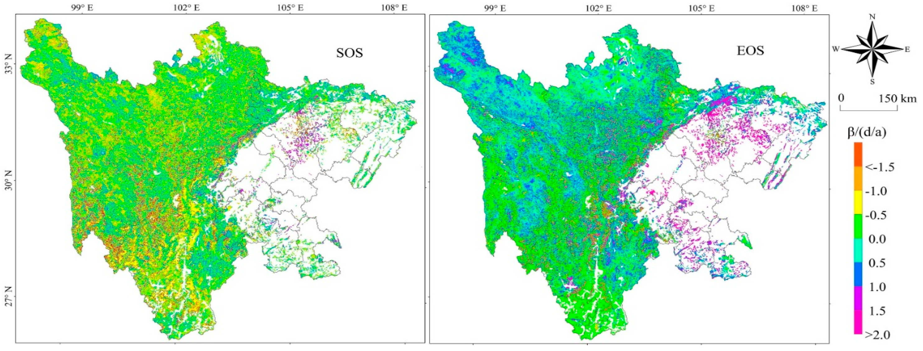
To fully understand the dynamic patterns of grassland phenology in Sichuan Province, we examined the phenology of grassland vegetation at the pixel level using MATLAB software and a combination of Theil–Sen trend analysis and Mann–Kendall tests (Figure 4). From 2001 to 2020, vegetation SOS of Sichuan Province was mainly concentrated in the 80–140 d period (61.83% of pixels). SOS advanced gradually, with the most obvious trend concentrated in the northwestern Sichuan Plateau. The average advance rate throughout the study area was basically above 1.0 d/a. 38.17% of SOS exhibited a delayed trend distributed among the mountainous area of southwest Sichuan, the Chengdu Plain, and the eastern Sichuan Basin Plain. The region with the highest delay rates was the Chengdu Plain, followed by the eastern Sichuan Basin Plain and the mountainous area of southwest Sichuan. The overall average delay rate was concentrated above 1.0 d. From the perspective of different vegetation types, steppe, deciduous forest, and coniferous forest lagged at the rates of 0.656 d, 0.241 d, and 0.168 d, respectively, but SOS showed a significant trend of advance from 2006 to 2007. Shrub, tussock, meadow, coniferous and broad-leaved mixed forest, and alpine vegetation all showed an insignificant advance trend. Among them, the advance rate of tussock was the highest, with an average advance rate of 0.182 d.
In Sichuan province, 71.32% of the vegetation EOS showed a lagging trend (67.13% of the total pixels by the significance test, p = 0.05). The regions with the highest EOS delay rate were concentrated around the eastern Sichuan Basin Plain, and the average delay rate in 20 years was over 1.5 d. The areas where EOS showed an early trend were concentrated in the mountainous area of southwestern Sichuan and the areas bordering Tibet on the northwestern Sichuan Plateau, and the lag rate was 0–0.5 d/a. The curves of interannual variation of different vegetation types all show a significant trend of lag. The vegetation type with the most significant lag trend was steppe, with an average lag rate of 0.894 d, followed by coniferous forest, with an average lag rate of 0.542 d. The vegetation type with the least lag rate was shrub, with an average lag rate of 0.372 d, followed by meadow, with an average lag rate of 0.426 d. The EOS change curve of alpine vegetation is clearly jagged.
3.4. Analysis of the Future Viability of the Phenological Period
Analysis of the sustainability of vegetation SOS and EOS in Sichuan Province from 2001 to 2020 was performed using the Hurst index (Figure 5). The future change trend of vegetation SOS in Sichuan Province exhibits a Hurst phenomenon with an average Hurst value of 0.44, i.e., the change trend of vegetation SOS in the future will have a weak opposite trend to the change trend in the period 2001–2020, i.e., vegetation SOS may be delayed. In 88.81% of the pixels, the Hurst index was between 0 and 0.5. Except for the pixels with Hurst index more than 0.5 in the eastern Sichuan Basin Plain, the Hurst index in the other regions (northwest Sichuan Plateau, Chengdu plain and mountainous area of southwestern Sichuan) was basically less than 0.5. The number of pixels with Hurst = 0.5 accounted for 3.15% of the total number of pixels, indicating that the change of vegetation SOS on a few pixels has nothing to do with the vegetation SOS in the period 2001–2020.
From 2001 to 2020, pixels with a Hurst value of more than 0.5 of the trend of vegetation change EOS in Sichuan Province accounted for 23.16% of the total pixels and they were concentrated in the Sichuan basin and mountainous regions in southwest Sichuan. The sustainability of vegetation EOS indicates that in the future, Sichuan province will continue the trend of the average level of change over the past 20 years and a shift will occur. Pixels below 0.5 account for 75.54% of the total pixels, which means that 75.54% of the pixel changes of EOS are opposite to the past and will have an upward trend in the future.
3.5. The Significant Influence of Extreme Climate Indices on Phenological Variables
The random forest regression model can convert the value of a variable into an integer, with larger values indicating higher significance. The model was used in this study to see how the fifteen extreme climate indices (Table 1) affect the parameters of vegetation phenology in Sichuan Province (Figure 6). The significant effects of several extreme climate indices on the changes of different vegetation phenology characteristics were different. SOS was mainly influenced by the yearly maximum consecutive five-day precipitation (RX5), diurnal temperature range (DTR), and temperature vegetation drought index (TVDI), with over 40% Inc MSE. EOS was mainly influenced by the yearly minimum value of daily minimum temperature (TNN), yearly mean value of temperature (TEMP_MEAN), and temperature vegetation dryness index (TVDI), with over 30% Inc MSE. The model was used here to determine the effects of extreme climate indices (Table 1) on various parameters of vegetation phenology in Sichuan Province. The focus was on the response of SOS, EOS, and overall regional vegetation phenology to extreme climate indices (Figure 6).
Therefore, the five extreme climate indices (RX5, DTR, TDVI, TNN, and TEMP_MEAN) were selected for the subsequent ridge regression sensitivity analysis based on the importance of the fifteen climate indices to vegetation phenology (Figure 7).
3.6. Analysis of Phenology Sensitivity to Extreme Climate Indices
The spatial distribution of phenology sensitivity to extreme climate indices (yearly maximum consecutive five-day precipitation (RX5), diurnal temperature range (DTR), yearly minimum value of daily minimum temperature (TNN), yearly mean value of temperature (TEMP_MEAN), and temperature vegetation dryness index (TVDI) in Sichuan Province from 2001 to 2020 were evaluated (Figure 7). Vegetation phenology showed different spatial differentiation concerning the five climate indices. The phenology measures SOS and EOS showed different spatial distributions with respect to the five climate indices (RX5, DTR, TVDI, TNN, TEMP_MEAN, and TVDI), respectively. The sensitivity coefficient of SOS was positive, while that of EOS was negative. The indices of yearly maximum consecutive five-day precipitation (RX5) and temperature vegetation dryness (TVDI) showed a positive sensitivity coefficient for SOS, and diurnal temperature range (DTR) showed negative sensitivity coefficient for SOS (Figure 7a). The yearly minimum value of daily minimum temperature (TNN) index showed a positive sensitivity coefficient for EOS in the mountainous area of southwestern Sichuan and a negative sensitivity coefficient for EOS in other regions (northwest Sichuan Plateau, Chengdu Plain and eastern Sichuan Basin Plain). The yearly mean values of temperature (TEMP_MEAN) and temperature vegetation dryness index (TVDI) showed a negative sensitivity coefficient for EOS in the mountainous area of southwestern Sichuan. The spatial distribution of the coefficients was relatively consistent, but not significant. The temperature vegetation dryness index (TVDI) was negative in northwest Sichuan Plateau and Chengdu Plain. The sensitivity coefficients of phenology for temperature indices were significantly higher than those for precipitation indices. The temperature vegetation dryness index (TVDI) showed positive and negative sensitivity to SOS and EOS, respectively.
4. Discussion
4.1. The Relationship between Grassland SOS and EOS, and Ground Observation and Remote Sensing Inversion Methods
According to Shen et al. [11], temporal trends in SOS differ significantly between remote sensing data and ground observations. Shen et al. [11] studied the phenological responses of plants to climate change on the Tibetan Plateau Satellite and found that remote sensing can only capture the leaf phenology of those species that are strongly represented in a community at the time of observation. If the sequence of leaf unfolding changes for different species within a community due to changing environmental conditions, the species with the highest cover at a given time may change. Satellite-based SOS is based on the greenness of a pixel, whereas ground-based observations are based on the morphological changes of individual plants. In evaluating satellite-based remote sensing of foliage phenology, the first problem is the data quality of the NDVI. Satellite images are usually acquired around midday and are contaminated by the target indicator, as well as by inaccurate atmospheric correction procedures for the sensors. In addition, the spectral configuration can be refracted and scattered by atmospheric components such as water vapor [62] and aerosols [63], leading to errors. Validation of satellite-based phenology is usually based on ground observations of phenology in cropland and deciduous forests at the species level [45]. In comparison, it is difficult to validate satellite-based phenology in natural grasslands using such species-level observations because a large number of species coexist within a pixel and have different phenological stages. Shen et al. (2015) determined the timing of spring green-up for the years 1982 to 1999 from data obtained from AVHRR NDVI using five different methods and for the years 2000 to 2011 using the same five methods from NDVIs observed by AVHRR, MODIS, and SPOT, and at MODIS EVI. The AVHRR sensor was renewed in late 2000 and since then it is suspected that the quality of the data from AVHRR NDVI had decreased from 2001 onwards [64]; the spring vegetation data of Zhang et al. [64] consist of three periods: from 1982 to 1997, obtained from the data of AVHRR NDVI, for 1998–1999, from the AVHRR and SPOT NDVI data, and from 2000–2011, from the NDVI datasets observed by MODIS and SPOT. For 1982–2011, consistent variability was found between SOS and remote sensing-based results. Che et al. [65] investigated the interannual variability of the averaged growing season end dates extracted from AVHRR LAI data on the Tibetan Plateau during 1982–2011 and Yu et al. [43] investigated the averaged growing season end dates of meadows extracted from AVHRR NDVI on the Tibetan Plateau. The extracted EOS showed a high degree of correspondence. In this study, the NDVI from MOD13A1 was used and the validation results showed that remotely sensed vegetation data SOS and EOS had earlier dates than the ground-based observations, with an error of less than 10 days between the remotely sensed and ground-based measurements of phenology; however, the results were still well correlated.
4.2. Trends in Grassland SOS and EOS
The change in the phenology of grasslands is a cyclical and continuous dynamic process. Many factors influence phenological change and there are certain relationships among the different factors. Cong et al. [66] and Slayback et al. [67] studied the phenological dynamics of different grasslands types in the northern Hemisphere from 1982 to 2009 and found that the evolution of grassland vegetation is more significant than that of forest vegetation over many years. The study found that the rate of phenological change in steppe was the largest among all vegetation types, followed by tussock vegetation, which is consistent with the conclusions of the study by Cong et al. [66]. Studies have shown that the rate of phenological change is significantly higher in grassland vegetation than in forests. The main reason for this is that grasslands are sensitive to climate change. Therefore, the increase in average temperature and the occurrence of climate extremes in recent years directly affect the productivity and carbon balance of grasslands. As a result of global warming, the SOS of grassland vegetation has changed drastically, leading to a shift in the global carbon cycle and climate adaptation [66,68]. Our research results also show that SOS of grassland vegetation was significantly delayed and EOS advanced. The differences in reported phenological changes among studies might be related to the different climatic conditions and vegetation types in the study areas [69].
4.3. The Relationship between Grassland Phenology and Extreme Climate Indices
Extreme temperature events influence vegetation growth and development by affecting the activities of photosynthetic and respiratory enzymes [18]. Extreme rainfall events inhibit growth by reducing the amount of available water in the soil where vegetation develops [69]. According to Piao et al. [41], high temperatures had a greater impact on northern vegetation than precipitation. Nagy et al. [16] found that extreme climate indices affect phenology. They pointed out that the flowering dates of temperate vegetation were almost one month earlier and some plant species could not complete their flowering cycle, but high precipitation events had little effect on the phenology of the observed plants. The sensitivity of phenological responses of different vegetation types to extreme climatic events is complicated. We found that the sensitivity of SOS was mainly influenced by the yearly maximum consecutive five-day precipitation (RX5), diurnal temperature range (DTR), and temperature vegetation dryness index (TVDI), while EOS was mainly influenced by the yearly minimum value of daily minimum temperature (TNN), yearly mean value of temperature (TEMP_MEAN), and TVDI. The SOS showed a negative sensitivity coefficient for DTR. If the diurnal temperature difference causes grassland phenology to begin earlier in the spring, this will lead to an earlier end of the growing season in the fall. SOS showed an advancing trend that could be attributed to warming, as the greater difference between TEMP_MAX and TEMP_MIN could favor growth. The increase in yearly maximum consecutive five-day precipitation (RX5) delayed the SOS, as cumulative precipitation is not a reliable measure of crop water supply. The timing and intensity of precipitation, soil freeze/thaw, snowmelt, evaporation, and permafrost decomposition can alter water availability and thus phenology. Unusual warming can boost plant activity, but this is not beneficial for vegetation development, as it leads to an early end of the growing season and shortens the vegetation growth cycle, as plants need to be exposed to lower temperatures before the end of the dormant period. Another possibility is that when vegetation is stressed by the environment, it uses its ever-changing signals—mainly hormones and signaling molecules—to regulate phenology, such as germination, leaf senescence, and growth stagnation. To protect itself from environmental stress, vegetation ends its growing season early. Moreover, a harsh climate is expected to make the seasonal trajectories of vegetative activities more vulnerable [70,71]. Vegetation phenology is both a periodic and a continuously dynamic process influenced by several interrelated influencing factors [34,72]. According to some studies, climate change is the most important element affecting vegetation phenology [72,73]. In this study, we focused on phenological changes caused by extreme climate indices, but we discovered during the analysis that the advance of vegetation SOS can indirectly lead to the advance of vegetation EOS. If vegetation EOS is affected by extreme climate indices in one year, it may also lead to changes in vegetation SOS in the following year. For this reason, we conducted a correlation analysis between SOS and EOS and the four seasons in this study (Figure 8).
There was a positive correlation between vegetation SOS and precipitation in four seasons (spring, summer, autumn, and winter). SOS had a significant negative correlation with temperature in spring and summer and a positive correlation with temperature in autumn and winter. EOS was negatively correlated with temperature in summer and winter and positively correlated with precipitation in summer, autumn, and winter.
4.4. Limitations
This study examines how grassland vegetation was affected by extreme climatic factors in Sichuan Province. However, grassland types are numerous and exhibit considerable vertical zonality, and different grassland types and flowering functional groups vary in sensitivity to changes in environmental factors in Sichuan. Grasslands were more vulnerable to climate change compared to other vegetation types [74,75]. Therefore, studying areas with low climate variability may be valuable for assessing the effects of climate change on grassland vegetation phenology. In addition, the effects of precipitation and temperature accumulation on plant phenophase should be further investigated. Other factors affecting vegetation in drylands are the timing and duration of precipitation [76], the water storage capacity of the soil, and evapotranspiration [77]. In addition to meteorological considerations, grassland phenology is influenced by a variety of environmental factors, including freeze-thaw processes, extreme weather events, atmospheric CO2 concentrations, and their combined impacts [78,79,80]. In this study, the future trend of vegetation dynamics is also quantified using the Hurst exponent, although the close correlation between future and past trends of vegetation dynamics was also found in the case study. However, the R/S analysis proposed in this study using the Hurst exponent could not answer the following question: how long do you think the expected trend in vegetation dynamics will last? It was more important to emphasize that time must be considered in predicting future vegetation dynamics. Future research in Sichuan Province will focus on gaining a full understanding of the combined environmental influences on grassland phenology. In addition, further case studies and theoretical research should be conducted on the detailed processes of future vegetation types.
5. Conclusions
The study discussed in this paper analyzes fifteen extreme climate indices in Sichuan Province using daily maximum and minimum temperatures and precipitation data from 38 meteorological stations from 2001 to 2020. The study highlights the spatio-temporal patterns and changing trends of vegetation phenology in the study area using NDVI from MOD13A1 data, and addresses the effects of climate events and trends on vegetation phenology. The results showed:
- The SOS vegetation in Sichuan Province gradually evolves with the geography of the slopes from west to east and from the surrounding mountains to the core basin. Climatic changes are strongly dependent on elevation, with most vegetation in the study area showing a trend of advancing SOS. Phenological EOS values of the different vegetation types differed and showed a trend towards delayed EOS. The development of grassland vegetation SOS was gradually delayed from mid to high altitudes, while it advanced at EOS. The tendency towards delayed SOS could be caused by insufficient cooling due to the warming climate in late autumn and winter.
- The future viability of grassland based on Hurst exponents showed that the changing trend of SOS and the changing trend between 2001 and 2020 were generally weak and opposite; i.e., grassland SOS could be delayed, which means that future trends are more random and have no clear direction. Pixels with a Hurst exponent greater than 0.5 in the Sichuan Basin indicate that the sustainability of vegetation EOS in the future will continue the same trend as the average level of change over the past 20 years, and there will be a shifting trend. To avoid the risk of ecological degradation, we need to take a series of measures to protect the plateau ecosystem: environmental protection projects should be further promoted, natural ecological reserves should be established, local people’s awareness of environmental protection and nature conservation should be raised, afforestation and artificial grassland construction should take place, and excessive development should be avoided. In addition, reasonable resource planning and allocation will help to better manage environmental security problems in the province.
- Grassland SOS was mainly influenced by the yearly maximum consecutive five-day precipitation, diurnal temperature, and temperature-vegetation dryness index, while EOS was mainly influenced by yearly minimum daily temperature, yearly mean temperature, and temperature-vegetation dryness index. Vegetation phenology in Sichuan province showed heterogeneous regional differentiation in response to different climate indices, with positive sensitivity coefficients between SOS and the climate indices compared to negative sensitivity coefficients between EOS and the climate indices. This suggests that extreme climate change leading to an advance in vegetation SOS may indirectly leads to an advance in vegetation EOS. SOS and EOS were strongly influenced by extreme climate and drought, implying that high temperatures lead to evaporation of moisture from the soil, resulting in a lack of rainfall leading to drought. SOS correlated positively with the yearly maximum consecutive five-day precipitation and temperature-vegetation dryness index, implying that precipitation and drought had a strong influence on vegetation growth.
Author Contributions
Writing—review and editing, B.A. and G.Q.; supervision, C.L. and J.W. All authors have read and agreed to the published version of the manuscript.
Funding
This work was supported by the National Natural Science Foundation of China (Grant No. 31760693).
Institutional Review Board Statement
Not applicable.
Informed Consent Statement
Not applicable.
Data Availability Statement
Not applicable.
Conflicts of Interest
The authors declare no conflict of interest.
References
- Lieth, H. Purposes of a phenology book. In Phenology and Seasonality Modeling; Springer: Berlin/Heidelberg, Germany, 1974; pp. 3–19. [Google Scholar]
- Schwartz, M.D. Phenology: An Integrative Environmental Science; Springer: Berlin/Heidelberg, Germany, 2003. [Google Scholar]
- Lee, H. Intergovernmental Panel on Climate Change. 2007. Available online: https://www.ipcc.ch/site/assets/uploads/2018/03/ar4_wg2_full_report.pdf (accessed on 2 December 2021).
- Qin, D. Climate change science and sustainable development. Prog. Geogr. 2014, 33, 874–883. [Google Scholar]
- IPCC. The Physical Science Basis, Summary for Policymakers, Contribution of WGI to the Fifth Assessment Report of the Intergovernmental Panel on Climate Change, 2013; Cambridge University Press: Cambridge, UK, 24 March 2014. [Google Scholar]
- Pei, T.; Ji, Z.; Chen, Y.; Wu, H.; Hou, Q.; Qin, G.; Xie, B. The Sensitivity of Vegetation Phenology to Extreme Climate Indices in the Loess Plateau, China. Sustainability 2021, 13, 7623. [Google Scholar] [CrossRef]
- Huang, H.; Zhang, B.; Huang, T.; Wang, H.-j.; Ma, B.; Wang, X.-d.; Cui, Y.-q. Quantifying and predicting spatial and temporal variations in extreme temperatures since 1990 in Gansu Province, China. Arid Land Geogr. 2020, 43, 319–328. [Google Scholar]
- Siegmund, J.F.; Wiedermann, M.; Donges, J.F.; Donner, R.V. Impact of temperature and precipitation extremes on the flowering dates of four German wildlife shrub species. Biogeosciences 2016, 13, 5541–5555. [Google Scholar] [CrossRef] [Green Version]
- Duan, H.; Xue, X.; Wang, T.; Kang, W.; Liao, J.; Liu, S. Spatial and Temporal Differences in Alpine Meadow, Alpine Steppe and All Vegetation of the Qinghai-Tibetan Plateau and Their Responses to Climate Change. Remote Sens. 2021, 13, 669. [Google Scholar] [CrossRef]
- Yang, B.; He, M.; Shishov, V.; Tychkov, I.; Vaganov, E.; Rossi, S.; Ljungqvist, F.C.; Bräuning, A.; Grießinger, J. New perspective on spring vegetation phenology and global climate change based on Tibetan Plateau tree-ring data. Proc. Natl. Acad. Sci. USA 2017, 114, 6966–6971. [Google Scholar] [CrossRef] [PubMed] [Green Version]
- Shen, M.; Piao, S.; Dorji, T.; Liu, Q.; Cong, N.; Chen, X.; An, S.; Wang, S.; Wang, T.; Zhang, G. Plant phenological responses to climate change on the Tibetan Plateau: Research status and challenges. Natl. Sci. Rev. 2015, 2, 454–467. [Google Scholar] [CrossRef] [Green Version]
- Richardson, A.D.; Andy Black, T.; Ciais, P.; Delbart, N.; Friedl, M.A.; Gobron, N.; Hollinger, D.Y.; Kutsch, W.L.; Longdoz, B.; Luyssaert, S. Influence of spring and autumn phenological transitions on forest ecosystem productivity. Philos. Trans. R. Soc. B Biol. Sci. 2010, 365, 3227–3246. [Google Scholar] [CrossRef] [PubMed] [Green Version]
- Barichivich, J.; Briffa, K.; Osborn, T.; Melvin, T.; Caesar, J. Thermal growing season and timing of biospheric carbon uptake across the Northern Hemisphere. Glob. Biogeochem. Cycles 2012, 26. [Google Scholar] [CrossRef]
- Keenan, T.F.; Gray, J.; Friedl, M.A.; Toomey, M.; Bohrer, G.; Hollinger, D.Y.; Munger, J.W.; O’Keefe, J.; Schmid, H.P.; Wing, I.S. Net carbon uptake has increased through warming-induced changes in temperate forest phenology. Nat. Clim. Chang. 2014, 4, 598–604. [Google Scholar] [CrossRef]
- Piao, S.; Tan, J.; Chen, A.; Fu, Y.H.; Ciais, P.; Liu, Q.; Janssens, I.A.; Vicca, S.; Zeng, Z.; Jeong, S.-J. Leaf onset in the northern hemisphere triggered by daytime temperature. Nat. Commun. 2015, 6, 6911. [Google Scholar] [CrossRef] [Green Version]
- Nagy, L.; Kreyling, J.; Gellesch, E.; Beierkuhnlein, C.; Jentsch, A. Recurring weather extremes alter the flowering phenology of two common temperate shrubs. Int. J. Biometeorol. 2013, 57, 579–588. [Google Scholar] [CrossRef] [PubMed]
- Bokhorst, S.; Tømmervik, H.; Callaghan, T.V.; Phoenix, G.K.; Bjerke, J.W. Vegetation recovery following extreme winter warming events in the sub-Arctic estimated using NDVI from remote sensing and handheld passive proximal sensors. Environ. Exp. Bot. 2012, 81, 18–25. [Google Scholar] [CrossRef]
- Xie, Y.; Wang, X.; Silander, J.A. Deciduous forest responses to temperature, precipitation, and drought imply complex climate change impacts. Proc. Natl. Acad. Sci. USA 2015, 112, 13585–13590. [Google Scholar] [CrossRef] [Green Version]
- Ying, H.; Zhang, H.; Zhao, J.; Shan, Y.; Zhang, Z.; Guo, X.; Rihan, W.; Deng, G. Effects of spring and summer extreme climate events on the autumn phenology of different vegetation types of Inner Mongolia, China, from 1982 to 2015. Ecol. Indic. 2020, 111, 105974. [Google Scholar] [CrossRef]
- Ciais, P.; Reichstein, M.; Viovy, N.; Granier, A.; Ogée, J.; Allard, V.; Aubinet, M.; Buchmann, N.; Bernhofer, C.; Carrara, A. Europe-wide reduction in primary productivity caused by the heat and drought in 2003. Nature 2005, 437, 529–533. [Google Scholar] [CrossRef]
- Cleland, E.E.; Chuine, I.; Menzel, A.; Mooney, H.A.; Schwartz, M.D. Shifting plant phenology in response to global change. Trends Ecol. Evol. 2007, 22, 357–365. [Google Scholar] [CrossRef]
- Haoming, X.; Ainong, L.; Wei, Z.; Jin, H.; Lei, G.; Bian, J.; Tan, J. Spatio-temporal variation and driving forces in alpine grassland phenology in the Zoigê plateau from 2001–2013. In Proceedings of the 2014 International Symposium on Geoscience and Remote Sensing (IGARSS), Quebec City, QC, Canada, 13–18 July 2014. [Google Scholar]
- Luo, X.; Yang, W.; Liu, L.; Zhang, Y. Spatial-Temporal variations of vegetation and the relationship with precipitation in the summer—A case study in the hilly area of central Sichuan province. In Proceedings of the 2018 3rd International Conference on Advances in Energy and Environment Research (ICAEER 2018), Guilin, China, 10–12 August 2018; p. 03060. [Google Scholar]
- Huang, J.; Sun, S.; Xue, Y.; Li, J.; Zhang, J. Spatial and temporal variability of precipitation and dryness/wetness during 1961–2008 in Sichuan province, west China. Water Resour. Manag. 2014, 28, 1655–1670. [Google Scholar] [CrossRef]
- Wang, S.; Jiao, S.; Xin, H. Spatio-temporal characteristics of temperature and precipitation in Sichuan Province, Southwestern China, 1960–2009. Quat. Int. 2013, 286, 103–115. [Google Scholar] [CrossRef]
- Li, Z.; He, Y.; Wang, C.; Wang, X.; Xin, H.; Zhang, W.; Cao, W. Spatial and temporal trends of temperature and precipitation during 1960–2008 at the Hengduan Mountains, China. Quat. Int. 2011, 236, 127–142. [Google Scholar] [CrossRef]
- Li, J.; Feng, Z.; Kang, J. Glacial deposits and environment in the Hengduan Mountains. In Glaciers in the Hengduan Mountains; Li, J., Su, Z., Eds.; Science Press: Beijing, China, 1996; pp. 157–173. [Google Scholar]
- Xu, Y.; Gao, X.; Shen, Y.; Xu, C.; Shi, Y.; Giorgi, A. A daily temperature dataset over China and its application invalidating an RCM simulation. Adv. Atmos. Sci. 2009, 26, 763–772. [Google Scholar] [CrossRef]
- Dong, Q.; Zhan, C.; Wang, H.; Wang, F.; Zhu, M. A review on evapotranspiration data assimilation based on hydrological models. J. Geogr. Sci. 2016, 26, 230–242. [Google Scholar] [CrossRef] [Green Version]
- Kong, J.; Hu, Y.; Yang, L.; Shan, Z.; Wang, Y. Estimation of evapotranspiration for the blown-sand region in the Ordos basin based on the SEBAL model. Int. J. Remote Sens. 2019, 40, 1945–1965. [Google Scholar] [CrossRef]
- Hou, X.; Gao, S.; Niu, Z.; Xu, Z. Extracting grassland vegetation phenology in North China based on cumulative SPOT-VEGETATION NDVI data. Int. J. Remote Sens. 2014, 35, 3316–3330. [Google Scholar] [CrossRef]
- He, Z.; Du, J.; Chen, L.; Zhu, X.; Lin, P.; Zhao, M.; Fang, S. Impacts of recent climate extremes on spring phenology in arid-mountain ecosystems in China. Agric. For. Meteorol. 2018, 260, 31–40. [Google Scholar] [CrossRef]
- Zhao, A.; Yu, Q.; Feng, L.; Zhang, A.; Pei, T. Evaluating the cumulative and time-lag effects of drought on grassland vegetation: A case study in the Chinese Loess Plateau. J. Environ. Manag. 2020, 261, 110214. [Google Scholar] [CrossRef] [PubMed]
- Kong, D.; Zhang, Q.; Huang, W.; Gu, X. Vegetation phenology change in Tibetan Plateau from 1982 to 2013 and its related meteorological factors. Acta Oceanol. Sin. 2017, 72, 39–52. [Google Scholar]
- Zhang, X.; Yang, F. RClimDex (1.0) User Manual; Climate Research Branch Environment Canada: Gatineau, QC, Canada, 10 September 2004; p. 22.
- Wang, H.; Pan, Y.; Li, S.; Chen, Z.; Zhao, Z.; Mi, H. Risk Assessment and Zonation of Meteorological Disasters Based on Rasterization in Jiangsu Province. J. Liaocheng Univ. Nat. Sci. Ed. 2019, 32, 99–110. [Google Scholar]
- Ranzi, R.; Caronna, P.; Tomirotti, M. Impact of climatic and land-use changes on river flows in the Southern Alps. In Sustainable Water Resources Planning and Management under Climate Change; Springer: Berlin/Heidelberg, Germany, 2017; pp. 61–83. [Google Scholar]
- Wills, A.; Mills, A.; Ninness, B. A matlab software environment for system identification. IFAC Proc. Vol. 2009, 42, 741–746. [Google Scholar] [CrossRef] [Green Version]
- Hutchinson, M.F.; Xu, T. Anusplin Version 4.2 User Guide; Centre for Resource and Environmental Studies, The Australian National University: Canberra, Australia, 2004; p. 54. [Google Scholar]
- Chen, J.; Jönsson, P.; Tamura, M.; Gu, Z.; Matsushita, B.; Eklundh, L. A simple method for reconstructing a high-quality NDVI time-series data set based on the Savitzky–Golay filter. Remote Sens. Environ. 2004, 91, 332–344. [Google Scholar] [CrossRef]
- Piao, S.; Fang, J.; Zhou, L.; Ciais, P.; Zhu, B. Variations in satellite-derived phenology in China’s temperate vegetation. Glob. Chang. Biol. 2006, 12, 672–685. [Google Scholar] [CrossRef]
- Zhou, L.; Tucker, C.J.; Kaufmann, R.K.; Slayback, D.; Shabanov, N.V.; Myneni, R.B. Variations in northern vegetation activity inferred from satellite data of vegetation index during 1981 to 1999. J. Geophys. Res. Atmos. 2001, 106, 20069–20083. [Google Scholar] [CrossRef]
- Yu, H.; Luedeling, E.; Xu, J. Winter and spring warming result in delayed spring phenology on the Tibetan Plateau. Proc. Natl. Acad. Sci. USA 2010, 107, 22151–22156. [Google Scholar] [CrossRef] [Green Version]
- Kafaki, S.B.; Mataji, A.; Hashemi, S.A. Monitoring growing season length of deciduous broadleaf forest derived from satellite data in Iran. Am. J. Environ. Sci. 2009, 5, 647–652. [Google Scholar]
- White, M.A.; Thornton, P.E.; Running, S.W. A continental phenology model for monitoring vegetation responses to interannual climatic variability. Glob. Biogeochem. Cycles 1997, 11, 217–234. [Google Scholar] [CrossRef]
- Hou, X.-H.; Niu, Z.; Gao, S. Phenology of forest vegetation in the northeast of China in ten years using remote sensing. Spectrosc. Spectr. Anal. 2014, 34, 515–519. [Google Scholar]
- Klosterman, S.; Hufkens, K.; Gray, J.; Melaas, E.; Sonnentag, O.; Lavine, I.; Mitchell, L.; Norman, R.; Friedl, M.; Richardson, A. Evaluating remote sensing of deciduous forest phenology at multiple spatial scales using PhenoCam imagery. Biogeosciences 2014, 11, 4305–4320. [Google Scholar] [CrossRef] [Green Version]
- Zhang, X.; Friedl, M.A.; Schaaf, C.B.; Strahler, A.H.; Hodges, J.C.; Gao, F.; Reed, B.C.; Huete, A. Monitoring vegetation phenology using MODIS. Remote Sens. Environ. 2003, 84, 471–475. [Google Scholar] [CrossRef]
- Sicard, P.; Mangin, A.; Hebel, P.; Malléa, P. Detection and estimation trends linked to air quality and mortality on French Riviera over the 1990–2005 period. Sci. Total Environ. 2010, 408, 1943–1950. [Google Scholar] [CrossRef]
- Zhang, A.; Zheng, C.; Wang, S.; Yao, Y. Analysis of streamflow variations in the Heihe River Basin, northwest China: Trends, abrupt changes, driving factors, and ecological influences. J. Hydrol. Reg. Stud. 2015, 3, 106–124. [Google Scholar] [CrossRef] [Green Version]
- Zhang, B.; He, C.; Burnham, M.; Zhang, L. Evaluating the coupling effects of climate aridity and vegetation restoration on soil erosion over the Loess Plateau in China. Sci. Total Environ. 2016, 539, 436–449. [Google Scholar] [CrossRef] [PubMed]
- Bayazit, M.; Önöz, B. To prewhiten or not to prewhiten in trend analysis? Hydrol. Sci. J. 2007, 52, 611–624. [Google Scholar] [CrossRef]
- Von Storch, H. Misuses of statistical analysis in climate research. In Analysis of Climate Variability; Springer: Berlin/Heidelberg, Germany, 1999; pp. 11–26. [Google Scholar]
- Yue, S.; Wang, C.Y. Applicability of prewhitening to eliminate the influence of serial correlation on the Mann-Kendall test. Water Resour. Res. 2002, 38, 4-1–4-7. [Google Scholar] [CrossRef]
- Carlson, T.N.; Gillies, R.R.; Perry, E.M. A method to make use of thermal infrared temperature and NDVI measurements to infer surface soil water content and fractional vegetation cover. Remote Sens. Rev. 1994, 9, 161–173. [Google Scholar] [CrossRef]
- Xu, K.; Yang, D.; Yang, H.; Li, Z.; Qin, Y.; Shen, Y. Spatio-temporal variation of drought in China during 1961–2012: A climatic perspective. J. Hydrol. 2015, 526, 253–264. [Google Scholar] [CrossRef]
- Sandholt, I.; Rasmussen, K.; Andersen, J. A simple interpretation of the surface temperature/vegetation index space for assessment of surface moisture status. Remote Sens. Environ. 2002, 79, 213–224. [Google Scholar] [CrossRef]
- Hurst, H.E. Long-term storage capacity of reservoirs. Trans. Am. Soc. Civ. Eng. 1951, 116, 770–799. [Google Scholar] [CrossRef]
- Mandelbrot, B.B.; Wallis, J.R. Robustness of the rescaled range R/S in the measurement of noncyclic long-run statistical dependence. Water Resour. Res. 1969, 5, 967–988. [Google Scholar] [CrossRef]
- Mandelbrot, B.B.; Wallis, J.R. Some long-run properties of geophysical records. Water Resour. Res. 1969, 5, 321–340. [Google Scholar] [CrossRef] [Green Version]
- Walker, E.; Birch, J.B. Influence measures in ridge regression. Technometrics 1988, 30, 221–227. [Google Scholar] [CrossRef]
- Tanre, D.; Holben, B.N.; Kaufman, Y.J. Atmospheric correction algorithm for NOAA-AVHRR products: Theory and application. Inst. Electr. Electron. Eng. Trans. Geosci. Remote Sens. 1992, 30, 231–248. [Google Scholar] [CrossRef]
- Nagol, J.R.; Vermote, E.F.; Prince, S.D. Effects of an atmospheric variation on AVHRR NDVI data. Remote Sens. Environ. 2009, 113, 392–397. [Google Scholar] [CrossRef]
- Zhang, G.; Zhang, Y.; Dong, J.; Xiao, X. Green-up dates in the Tibetan Plateau have continuously advanced from 1982 to 2011. Proc. Natl. Acad. Sci. USA 2013, 110, 4309–4314. [Google Scholar] [CrossRef] [Green Version]
- Che, M.; Chen, B.; Innes, J.L.; Wang, G.; Dou, X.; Zhou, T.; Zhang, H.; Yan, J.; Xu, G.; Zhao, H. Spatial and temporal variations in the end date of the vegetation growing season throughout the Qinghai–Tibetan Plateau from 1982 to 2011. Agric. For. Meteorol. 2014, 189, 81–90. [Google Scholar] [CrossRef]
- Cong, N.; Shen, M.; Yang, W.; Yang, Z.; Zhang, G.; Piao, S. Varying responses of vegetation activity to climate changes on the Tibetan Plateau grassland. Int. J. Biometeorol. 2017, 61, 1433–1444. [Google Scholar] [CrossRef]
- Slayback, D.A.; Pinzon, J.E.; Los, S.O.; Tucker, C.J. Northern hemisphere photosynthetic trends 1982–99. Glob. Chang. Biol. 2003, 9, 1–15. [Google Scholar] [CrossRef]
- Liu, Q.; Fu, Y.H.; Zeng, Z.; Huang, M.; Li, X.; Piao, S. Temperature, precipitation, and insolation effects on autumn vegetation phenology in temperate China. Glob. Chang. Biol. 2016, 22, 644–655. [Google Scholar] [CrossRef] [PubMed]
- Lupascu, M.; Welker, J.; Seibt, U.; Xu, X.; Velicogna, I.; Lindsey, D.; Czimczik, C. The amount and timing of precipitation control the magnitude, seasonality, and sources (14 C) of ecosystem respiration in a polar semi-desert, northwestern Greenland. Biogeosciences 2014, 11, 4289–4304. [Google Scholar] [CrossRef] [Green Version]
- Butt, N.; Seabrook, L.; Maron, M.; Law, B.S.; Dawson, T.P.; Syktus, J.; McAlpine, C.A. Cascading effects of climate extremes on vertebrate fauna through changes to low-latitude tree flowering and fruiting phenology. Glob. Chang. Biol. 2015, 21, 3267–3277. [Google Scholar] [CrossRef] [PubMed] [Green Version]
- Crabbe, R.A.; Dash, J.; Rodriguez-Galiano, V.F.; Janous, D.; Pavelka, M.; Marek, M.V. Extreme warm temperatures alter forest phenology and productivity in Europe. Sci. Total Environ. 2016, 563, 486–495. [Google Scholar] [CrossRef]
- Xie, B.; Qin, Z.; Wang, Y.; Chang, Q. Monitoring vegetation phenology and their response to climate change on Chinese Loess Plateau based on remote sensing. Trans. Chin. Soc. Agric. Eng. 2015, 31, 153–160. [Google Scholar]
- Peñuelas, J.; Rutishauser, T.; Filella, I. Phenology feedbacks on climate change. Science 2009, 324, 887–888. [Google Scholar] [CrossRef] [PubMed] [Green Version]
- Liu, H.; Tian, F.; Hu, H.C.; Hu, H.P.; Sivapalan, M. Soil moisture controls on patterns of grass green-up in Inner Mongolia: An index-based approach. Hydrol. Earth Syst. Sci. 2013, 17, 805–815. [Google Scholar] [CrossRef] [Green Version]
- Wang, H. The variability of vegetation growing season in northern China based on NOAA NDVI and MSAVI from 1982 to 1999. Acta Ecol. Sin. 2007, 27, 504–515. [Google Scholar]
- Cong, N.; Wang, T.; Nan, H.; Ma, Y.; Wang, X.; Myneni, R.B.; Piao, S. Changes in satellite-derived spring vegetation green-update and its linkage to the climate in China from 1982 to 2010: A multimethod analysis. Glob. Chang. Biol. 2013, 19, 881–891. [Google Scholar] [CrossRef] [PubMed]
- Jin, H.; He, R.; Cheng, G.; Wu, Q.; Wang, S.; Lü, L.; Chang, X. Changes in frozen ground in the Source Area of the Yellow River on the Qinghai–Tibet Plateau, China, and their eco-environmental impacts. Environ. Res. Lett. 2009, 4, 045206. [Google Scholar] [CrossRef]
- Chen, H.; Zhu, Q.; Wu, N.; Wang, Y.; Peng, C.-H. Delayed spring phenology on the Tibetan Plateau may also be attributable to other factors than winter and spring warming. Proc. Natl. Acad. Sci. USA 2011, 108, E93. [Google Scholar] [CrossRef] [Green Version]
- Reyes-Fox, M.; Steltzer, H.; Trlica, M.; McMaster, G.S.; Andales, A.A.; LeCain, D.R.; Morgan, J.A. Elevated CO2 further lengthens growing season under warming conditions. Nature 2014, 510, 259–262. [Google Scholar] [CrossRef]
- Yang, Y.; Guan, H.; Shen, M.; Liang, W.; Jiang, L. Changes in autumn vegetation dormancy onset date and the climate controls across temperate ecosystems in China from 1982 to 2010. Glob. Chang. Biol. 2015, 21, 652–665. [Google Scholar] [CrossRef] [PubMed]
Figure 1.
(a) The geographical position of Sichuan Province; (b) a map of the types of vegetation in Sichuan Province; (c) a topographical map and the distribution of meteorological stations in Sichuan Province.
Figure 1.
(a) The geographical position of Sichuan Province; (b) a map of the types of vegetation in Sichuan Province; (c) a topographical map and the distribution of meteorological stations in Sichuan Province.

Figure 2.
Correlation of grassland vegetation (a) SOS and (b) EOS between the NDVI from MOD13A1 data and ground observations.
Figure 2.
Correlation of grassland vegetation (a) SOS and (b) EOS between the NDVI from MOD13A1 data and ground observations.

Figure 3.
Spatial distribution of annual mean phenological values ((a) Start of the season and (b) End of the season) and vegetation percentages ((c) Start of the season and (d) End of the season) of the eight grassland types (I: shrub; II: steppe; III;: tussock; IV: meadow; V: coniferous forest; VI: coniferous and broad-leaved mixed forest; VII: deciduous forest; VIII: alpine vegetation) in the Sichuan Province from 2001–2020.

Figure 4.
The trend of change in the spatial distribution of (a) grassland SOS, (b) grassland EOS, and the trend of interannual variation in vegetation phenology of SOS and EOS. (I: shrub; II: steppe; III: tussock; IV: meadow; V: coniferous forest; VI: coniferous and broad-leaved mixed forest; VII: deciduous forest; VIII: alpine vegetation).

Figure 5.
Analysis of the phenological sustainability of grasslands in Sichuan Province using the Hurst exponent (β(d/a).
Figure 5.
Analysis of the phenological sustainability of grasslands in Sichuan Province using the Hurst exponent (β(d/a).

Figure 6.
The importance of the climate indices for the phenological parameters start of the growing season (SOS) and end of the growing season (EOS), estimated as the percentage increase in the mean square error (% Inc MSE) of the different vegetation types.
Figure 6.
The importance of the climate indices for the phenological parameters start of the growing season (SOS) and end of the growing season (EOS), estimated as the percentage increase in the mean square error (% Inc MSE) of the different vegetation types.

Figure 7.
The sensitivity of vegetation phenology in Sichuan Province to extreme climate indices. The proportion of pixels with p < 0.01 is less than 10%. The sensitivity response of start of the growing season (SOS) to RX5 (a), the sensitivity response of SOS to DTR (b), the sensitivity response of SOS to TVDI (c), the sensitivity response of end of the growing season (EOS) to TNN (d), the sensitivity response of EOS to TEMP_MEAN (e), the sensitivity response of EOS to TVDI (f).

Figure 8.
Partial correlation analysis between SOS and EOS and precipitation and temperature over the four seasons with significance at the p = 0.05 level. Partial correlation between SOS and precipitation in (a) spring, (b) summer, (c) autumn, (d) winter; partial correlation between SOS and temperature in (e) spring, (f) summer, (g) autumn, (h) winter; partial correlation between EOS and precipitation in (i) spring, (j) summer, (k) autumn, (l) winter; partial correlation between EOS and temperature in (m) spring, (n) summer, (o) autumn, (p) winter.


Table 1.
The definitions and classifications of climate indices.
| Indicators | Description |
|---|---|
| DEM | Digital elevation model |
| RS | Solar radiation |
| ET | Evapotranspiration |
| TVDI | Temperature vegetation dryness index |
| PER | Yearly mean accumulated precipitation |
| RX1 | Yearly maximum consecutive one-day precipitation |
| RX5 | Yearly maximum consecutive five-day precipitation |
| DTR | Diurnal temperature range |
| TEMP_MEAN | Yearly mean value of temperature |
| TEMP_MAX | Yearly mean value of daily maximum temperature |
| TEMP_MIN | Yearly mean value of daily minimum temperature |
| TNN | Yearly minimum value of daily minimum temperature |
| TNX | Yearly maximum value of daily minimum temperature |
| TXN | Yearly minimum value of daily maximum temperature |
| TXX | Yearly maximum value of daily maximum temperature |
Publisher’s Note: MDPI stays neutral with regard to jurisdictional claims in published maps and institutional affiliations. |
© 2021 by the authors. Licensee MDPI, Basel, Switzerland. This article is an open access article distributed under the terms and conditions of the Creative Commons Attribution (CC BY) license (https://creativecommons.org/licenses/by/4.0/).
Share and Cite
MDPI and ACS Style
Adu, B.; Qin, G.; Li, C.; Wu, J. Grassland Phenology’s Sensitivity to Extreme Climate Indices in the Sichuan Province, Western China. Atmosphere 2021, 12, 1650. https://0-doi-org.brum.beds.ac.uk/10.3390/atmos12121650
AMA Style
Adu B, Qin G, Li C, Wu J. Grassland Phenology’s Sensitivity to Extreme Climate Indices in the Sichuan Province, Western China. Atmosphere. 2021; 12(12):1650. https://0-doi-org.brum.beds.ac.uk/10.3390/atmos12121650
Chicago/Turabian StyleAdu, Benjamin, Gexia Qin, Chunbin Li, and Jing Wu. 2021. "Grassland Phenology’s Sensitivity to Extreme Climate Indices in the Sichuan Province, Western China" Atmosphere 12, no. 12: 1650. https://0-doi-org.brum.beds.ac.uk/10.3390/atmos12121650
Note that from the first issue of 2016, this journal uses article numbers instead of page numbers. See further details here.