Article

Venus’ Cloud-Tracked Winds Using Ground- and Space-Based Observations with TNG/NICS and VEx/VIRTIS †

1
Institute of Astrophysics and Space Sciences, Observatório Astronómico de Lisboa, Ed. Leste, Tapada da Ajuda, 1349-018 Lisbon, Portugal
2
Institute of Space and Astronautical Science, Japan Aerospace Exploration Agency—3-1-1, Yoshinodai, Chuo-ku, Sagamihara 252-5210, Japan
3
Departamento de FAMN, Facultad de Física, Universidad de Sevilla, 41012 Seville, Spain
*
Author to whom correspondence should be addressed.
Based on Observations Made with the Italian Telescopio Nazionale Galileo (TNG) Operated on the Island of La Palma by the Fundación Galileo Galilei of the INAF (Istituto Nazionale di Astrofisica) at the Spanish Observatorio del Roque de los Muchachos of the Instituto de Astrofisica de Canarias.
Submission received: 20 December 2021 / Revised: 24 January 2022 / Accepted: 13 February 2022 / Published: 17 February 2022
(This article belongs to the Special Issue Planetary Atmospheres: From Solar System to Exoplanets)

Abstract

:
Characterizing the wind speeds of Venus and their variability at multiple vertical levels is essential for a better understanding of the atmospheric superrotation, constraining the role of large-scale planetary waves in the maintenance of this superrotation, and in studying how the wind field affects clouds’ distribution. Here, we present cloud-tracked wind results of the Venus nightside, obtained with unprecedented quality using ground-based observations during July 2012 with the near-infrared camera and spectrograph (NICS) of the Telescopio Nazionale Galileo (TNG) in La Palma. These observations were performed during 3 consecutive days for periods of 2.5 h starting just before dawn, sensing the nightside lower clouds of Venus close to 48 km of altitude with images taken at continuum K filter at 2.28 μ m. Our observations cover a period of time when ESA’s Venus Express was not able to observe these deeper clouds of Venus due to a failure in the infrared channel of its imaging spectrometer, VIRTIS-M, and the dates were chosen to coordinate these ground-based observations with Venus Express’ observations of the dayside cloud tops (at about 70 km) with images at 380 nm acquired with the imaging spectrometer VIRTIS-M. Thanks to the quality and spatial resolution of TNG/NICS images and the use of an accurate technique of template matching to perform cloud tracking, we present the most detailed and complete profile of wind speeds ever performed using ground-based observations of Venus. The vertical shear of the wind was also obtained for the first time, obtained by the combination of ground-based and space-based observations, during the Venus Express mission since the year 2008, when the infrared channel of VIRTIS-M stopped working. Our observations exhibit day-to-day changes in the nightside lower clouds, the probable manifestation of the cloud discontinuity, no relevant variations in the zonal winds, and an accurate characterization of their decay towards the poles, along with the meridional circulation. Finally, we also present the latitudinal profiles of zonal winds, meridional winds, and vertical shear of the zonal wind between the upper clouds’ top and lower clouds, confirming previous findings by Venus Express.

1. Introduction

The atmosphere of Venus is in superrotation, a state in which its averaged angular momentum is much greater than that corresponding to corotation with the surface. The circulation up to the cloud tops is characterised by an increasing zonal retrograde wind (in the east–west direction). The retrograde zonal superrotation (RZS) wind starts to build up at 10 km and amplifies with altitude, reaching a maximum at cloud tops (∼70 km), where the atmosphere rotates about 60 times faster than the surface [1].
At visible wavelengths, the Venus disk appears totally covered by thick clouds. Although the clouds are almost featureless in visible light, there are prominent features in UV and infrared wavelengths. The cloud deck extends in altitude from 45 to 70 km, and can be divided into 3 main regions, the lower cloud deck—centred at 48 km of altitude, extending from the cloud base, at an altitude of 44 up to roughly 50 km—the middle cloud deck, centred at 54 km (covering the altitude range from 50 to 55 km), and finally the upper cloud deck, centred at 60 km, spanning from 55 km to the cloud tops at nearly 70 km [2,3]. The lower cloud deck is where fundamental dynamical exchanges that help maintain superrotation are thought to occur [4].
Venus possesses an extremely dense atmosphere, if compared with Earth, with a surface pressure of 93 bars and a mean surface temperature of 735 K. The lower Venusian atmosphere is a strong source of thermal radiation, with the gaseous CO 2 component allowing radiation to escape in windows at 1.74 and 2.28 μ m. At these wavelengths, radiation originates below 35 km, and unit opacity is reached at the lower cloud level, close to 48 km. Therefore, in these windows, it is possible to observe the horizontal cloud structure, with thicker clouds seen silhouetted against the bright thermal background from the lower atmosphere. Our objective is to provide direct wind measurements and a map of cloud distribution at the lower cloud level in the Venus mesosphere, in order to complement Venus Express (VEx). VEx was a European space mission to Venus that was operative in the period April 2006–December 2014, including Akatsuki (Akatsuki is currently the only space mission monitoring the planet) and other ground-based observations of the cloud layer wind regime. By continuous monitoring of the horizontal cloud structure at 2.28 μ m (Kcont filter), it is possible to determine wind fields using the cloud tracking technique.
The motion of the cloud features is strongly correlated with the prevailing winds at their estimated altitude range [5]—while radiation at UV wavelengths is scattered at Venus’ dayside cloud tops, at nearly 70 km altitude, it is possible to sound the nightside bottom of the cloud level (48 km) using the 1.74 and 2.28 μ m NIR windows, which will sense the opacity variability of the clouds at these levels. The cloud tracking techniques, that follow the motion of the cloud patterns with time, allow the wind’s velocity field retrieval at different heights, contributing to study the dynamics of the Venus atmosphere.
In December 2015, JAXA’s Akatsuki mission (formerly Venus Climate Orbiter or VCO) successfully performed its Venus’ orbital insertion manoeuvre [6]. The Akatsuki’s equatorial orbit and its payload instruments—as is the case of the onboard infrared cameras IR1 and IR2, and the UVI instrument that senses Venus’ atmosphere in shorter wavelengths—performed observations that allowed important new discoveries regarding the Venus’ atmosphere dynamics [7,8,9].
Ground-based observations also contribute in a decisive way to a better understanding of the processes governing the atmosphere dynamics. On the one hand, ground-based observations improve the temporal baseline of space-based observations of Akatsuki and Venus Express, among others, allowing the continuation of long-term study of wind variability. On the other hand, the intrinsic complementarity of ground observations can improve the latitudinal coverage, or increase the quality of specific measurements due to the use of dedicated techniques, in the case of high-resolution spectroscopic Doppler methods that allowed researchers to retrieve meridional wind velocities with high precision [10,11,12].
First attempts to use ground-based, near-infrared Venus observations to explore nightside lower clouds include Allen and Crawford [13], Crisp et al. [14], and Chanover et al. [15]. The first relevant nightside dynamical results include Crisp et al. [16] and Limaye et al. [17], using ground-based, near-infrared observations (at 2.3 μ m transparency window), and Tavenner et al. [18], who produced a bottom cloud deck map relying on observations made with NASA’s Infrared Telescope Facility (IRTF). Early space-based contributions to the study of the wind field at the bottom clouds’ level include the results from Pioneer Venus entry probe and the observations carried out in the infrared domain from Galileo/NIMS [19]. From 2006, the southern hemisphere lower cloud deck was thoroughly studied with Venus Express (VEx) observations and the related wind field was explored with unprecedented precision [5,20,21].
Recently, with the advent of the Akatsuki space probe and its equatorial orbit, it was possible to analyse with great detail the clouds and dynamics of the lower-to-middle Venus’ atmosphere layers, in both hemispheres [22,23]. The accuracy of Akatsuki IR2 camera images were aligned with the long-term observations of the deep Venusian atmosphere, allowing researchers to retrieve striking new features, as this is the case in the planetary-scale, bow-shaped equatorial discontinuity [9] and the profusion of mesoscale vortices [23]. Since the IR1 and IR2 cameras stopped working in December 2016 [24], ground-based NIR observations constitute the only way of resuming the outstanding Akatsuki’s infrared atmospheric research.
Recent developments in ground-based techniques in enhancing the precision of the images obtained and improving accuracy in the images’ navigation (i.e., extreme precision in the attribution of latitude/longitude coordinates in the observed images from ground telescopes) allowed researchers to improve the contribution of ground-based NIR observations on Venus’ nightside lower cloud deck investigation. In fact, the use of an improved cloud tracking method, based on phase correlation between images [22], and the use of NASA SPICE kernels [25], combined with a more accurate adjustment of the planetary limb to the coordinates grid, increased the precision in the identification of telescope observation images’ pixel-related planetary coordinates.
The study of the lower cloud wind field (∼48–55 km), on both Venus’ hemispheres, could provide crucial hints in understanding the source of the atmospheric angular momentum excess that leads to the superrotation phenomena observed on Venus’ atmosphere. We note that, in the period between the failure of the visible and infrared thermal imaging spectrometer (VIRTIS) on board the Venus Express [26] infrared channel and the Akatsuki Venus’ orbital insertion, and after the Akatsuki/IR2 camera stopped working in 2016 [24], it was not possible to sense and study Venus’ dynamics at the bottom of the cloud level using space-based observations. We also note that the ground-based NIR dataset presented in this work is a unique way to study the Venus’ atmosphere dynamics at the cloud bottom layer for 2012.
Taking in account the relevance of presenting results from coordinated observations, coming from different instruments and wavelength ranges, we took advantage of a coordinated observational campaign between space-based VEx and ground-based observations with TNG/NICS. This multi-instrument and multi-technique observation method has largely proved its efficiency in previous studies [10,11,27,28,29].
In this work, we present nightside wind velocity results, these results were retrieved from ground-based TNG/NICS observations (see Figure 1) in the 2.28 μ m NIR windows sounding the bottom of the cloud level (∼48 km). Our observational efforts were coordinated with VEx/VIRTIS-M cloud tops dayside observations; therefore, we will also present simultaneous dayside winds measured at the cloud top level (∼70 km) and, finally, we will present a first approach to the vertical wind shear between the altitudes, sensed in the context of the present work. We will also compare the obtained results with GCM modelling predictions (LMD). The fact that the zonal wind at the bottom of the cloud layer is highly stable [30] allowed the researchers to present, here, an estimate of the vertical shear of the wind between the two altitudes sensed in the context of this study (the lower and top cloud layers).

2. Observations and Image Processing

In this work, we present results based on observations carried out with the near-infrared camera and spectrograph (NICS) of the Telescopio Nazionale Galileo (TNG), in La Palma, between 10 and 12 July 2012 (Figure 1). We observed for periods of 2.5 h starting just before dawn, for 3 consecutive nights (Figure 2 shows the observation’s geometry for each one of the observing days). We acquired a set of images of the nightside of Venus with the continuum K filter at 2.28 μ m ( k c o n t ), which allowed us to monitor motions at the lower cloud level of the atmosphere of Venus, close to 48 km altitude. We acquired a series of short exposures of the Venus disk (exposure time of 3 s). These observations were part of the network of ground-based observations of Venus coordinated with ESA’s Venus Express orbiter for the 2012 Venus transit campaign [31].

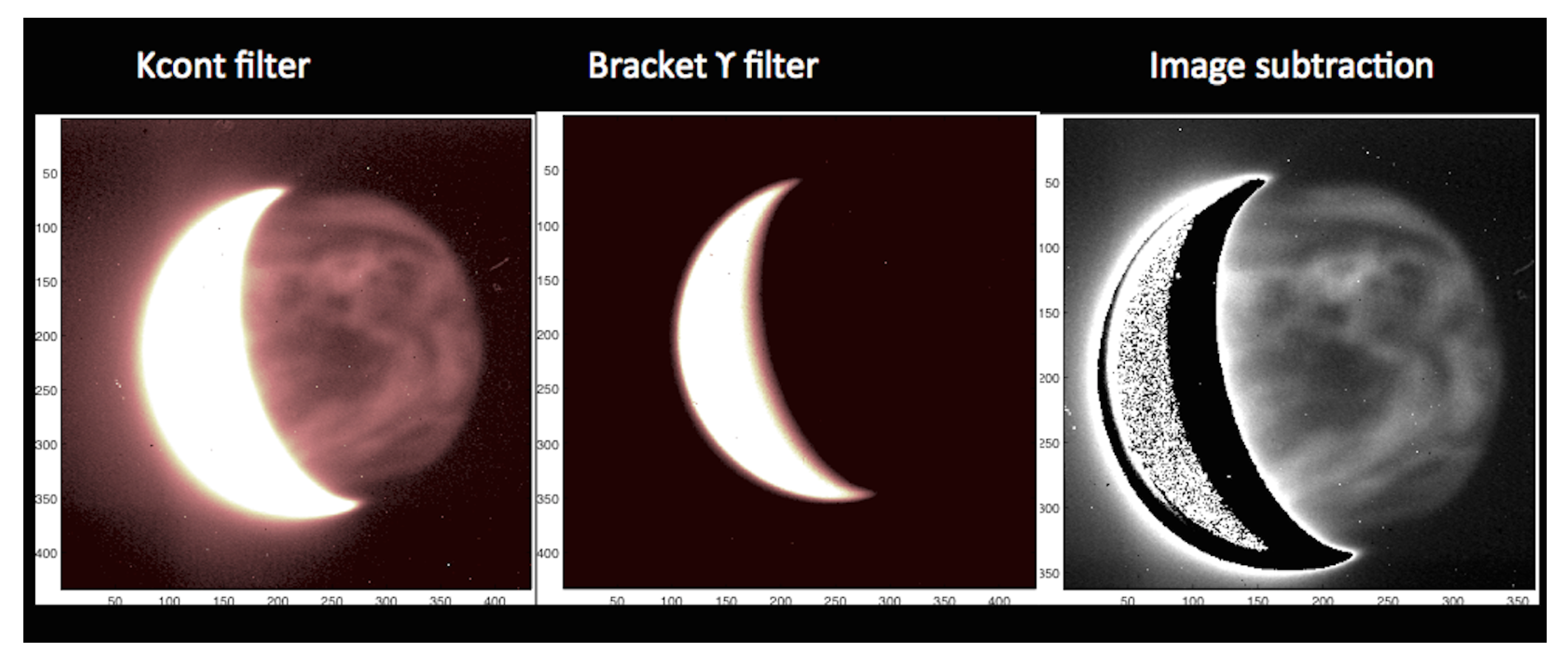
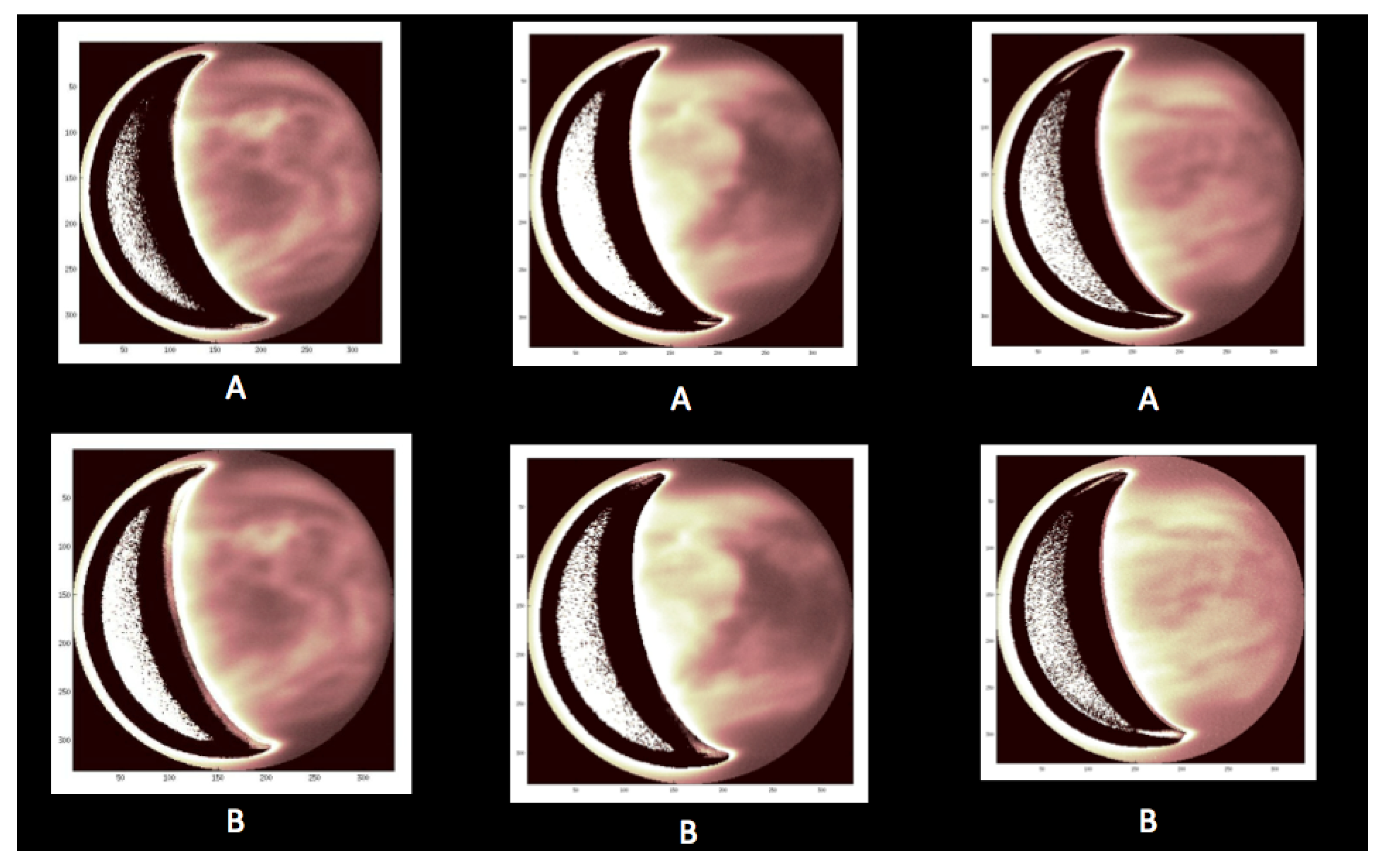
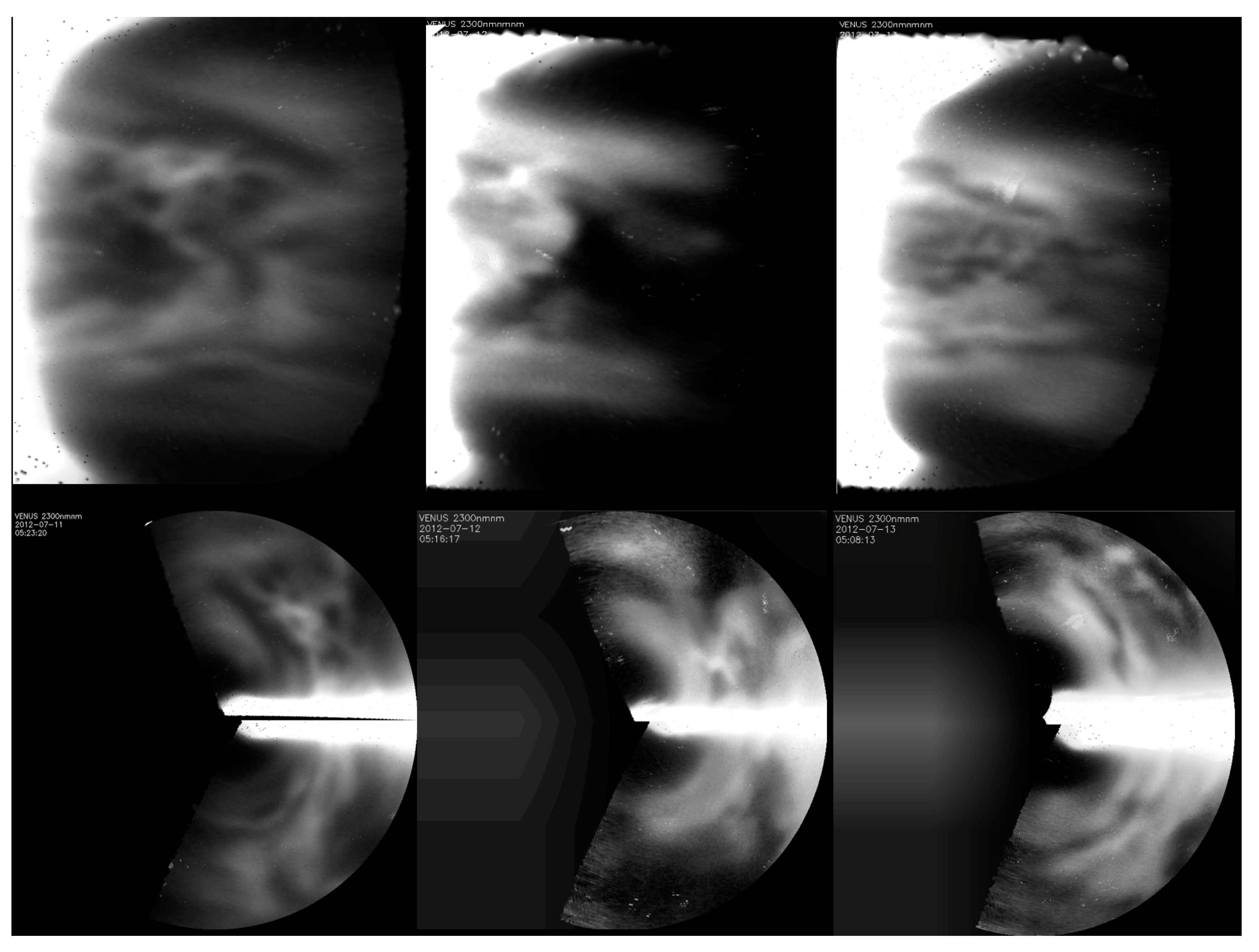
2.1. Ground-Based Observations with TNG/NICS

Venus’ apparent diameter at observational dates was greater than 36 arcsec, allowing a high spatial resolution. Even though the pixel scale of the NICS narrow field camera is 0.13 arcsec, the atmospheric seeing during our observations (ranging 0.8–1.0 arcsec) limited the effective spatial resolution of our images. Super-resolution imaging for Venus can be attained using the lucky imaging technique [32,33,34], and, in previous works, the lucky imaging technique allowed researchers to obtain stacked images of Venus that improved, by a factor of 3, the spatial resolution imposed by the atmospheric seeing [29]. In this work, we selected the best-aligned frames where turbulence was not present, stacked those frames, and obtained an ultra-high-resolution image below the typical seeing, though it was limited by the pixel size of the NICS camera. Lucky imaging has been proven to improve the spatial resolution under a varied set of seeing conditions [35], and although resolutions as small as 0.1 have been reported in some cases [36], we assessed that a more conservative resolution of 0.2 arcsec per pixel matched the resolution of our stacked images better. Note that this value is typical of the resolutions achieved at very high altitude observatories or with adaptive optics [37].
The absolute spatial resolution, averaged across the 3 days of observations, on the disk was ∼106 km/px at disk centre. Since the observing nights, we obtained two stacked images, obtained from sets of images separated by a time interval of about 60 min, assuming wind speeds of the order of 60 m/s [22] we expect that clouds would move approximately 216 km (above 2 pixels) between the pair of images.
In order to correct for scattered light from the (saturated) dayside crescent into the nightside, a set of observations with a Bracket gamma (Br γ ) filter, centred at 2.169 μ m, were performed (Figure 3). Cloud patterns are not observable with this filter due to the high optical depth of the gaseous CO 2 component. Subtracting k c o n t and Br γ images allowed us to efficiently correct the pollution due to this scattered light from the saturated dayside [18].
The correction of the scattered light with the Br γ images also helped to improve the visualization of the planetary limb and, hence, to obtain a more accurate position of the coordinates’ grid. Besides, co-adding the best images and cross-correlating regions of clouds (Figure 4) helped us to obtain an effective resolution significantly by overcoming the seeing-limited resolution.
In order to prevent image saturation, even on the nightside, when using the k c o n t filter, we used a Gray 5 attenuator filter (which reduces the flux between 4.8 and 5.7 magnitudes in the wavelength range from 1.03 to 2.15 μ m with a 0.3 magnitude accuracy).
On the other hand, since we started observing Venus still with low elevation (airmass ∼3), we were obliged to increase the exposure time at the beginning of each day, observing the run. Accordingly, the used exposure time was 10 s until the airmass reached approximately 2.5. With this caution, we could obtain—even at the beginning of each day’s run—images with enough contrast which allowed us to perform cloud tracking. With the steady decrease in the airmass, we were forced to use a 3 s exposure time to prevent nightside image saturation and maintain the optimal contrast at Venus’ lower cloud deck. Orbital geometry and observational characteristics are displayed on Table 1.

2.2. Coordinated Space-Based Observations with VEx/VIRTIS-M

VEx/VIRTIS-M is a 2-channel imaging spectrometer operating in the visible and infrared (0.3–1 μ m and 1–5 μ m) wavelength ranges [26]. The visible channel maps the dayside at ultraviolet wavelengths of about 380 nm, probing UV features at an altitude of 66–73 km. We selected pairs of VIRTIS-M ultraviolet (UV) images at 380 nm to retrieve wind speeds from the motions of the clouds on the dayside of Venus. To improve the measurement accuracy, the time interval between images was maximized (typically ∼1 h). The motions of the UV upper cloud features were visually measured on equirectangular projections of these VIRTIS-M images, which were previously processed to enhance the visualization of the cloud patterns following the same procedure as in previous works [21,38].
Coordinated VEx observations included in this work comprised a set of UV dayside images acquired during VEx orbit numbers from 2272 to 2273, during the days 11–12 of July 2012, respectively. Since the quality of these VEx/VIRTIS-M images was variable, we discarded the images with lower signal–noise ratio (SNR) for our purpose of measuring wind speeds by manually tracking cloud tracers. The selected pairs of images were separated by a time interval of around 60 min, encompassing a latitude range from the equator to 80 S. Planetary local hours spanned from 10 h to 17 h (see Table 2). These observations were chose to match the same observing dates as our ground-based observations with TNG/NICS (see Table 2).
The original VIRTIS-M images were navigated and processed to improve the SNR ratio using the convolution with the directional filter described by Hueso et al. [38]. As the position of the spacecraft changes along with the instant where each image was acquired, each couple of images were cylindrically or polar projected depending on whether they were sensing regions closer to the equator or to the South Pole. Figure 5 shows 2 examples of VIRTIS-M images at 380 nm after being processed and geometrically projected. In all the cases, a grid with a spatial resolution of 0.2 was employed.

3. Wind Determination Methods

Tracking the motions of the clouds in images has long been regarded as a trustworthy method for estimating the wind speeds of Venus within the cloud layer [3], and the results have been repeatedly validated by comparison with in situ measurements by entry probes and balloons [40]. For winds at the cloud tops (∼70 km above the surface), these are usually evaluated using UV images of the dayside of Venus [5,8,41,42], while for the deeper winds at the middle-to-lower clouds (approximately at 47.5–56.5 km of altitude), we use images of the dayside taken at visible and near-infrared wavelengths [42,43] and infrared images at bands 1.7 and 2.3 μ m for nightside clouds, seen as opacity patterns against the background emission from the deep atmosphere of Venus [3,17,22].

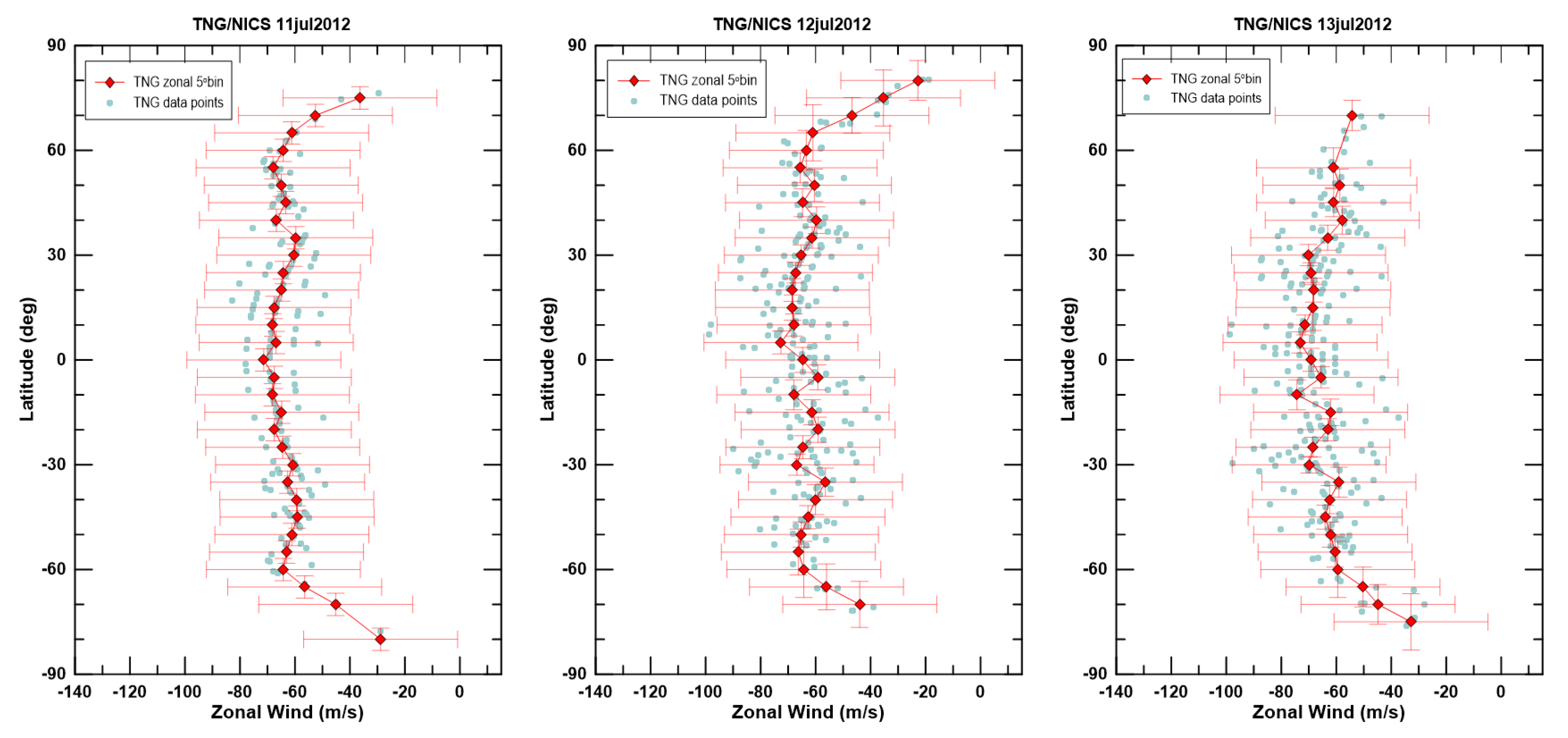
3.1. Cloud-Tracked Winds on the Nightside Using TNG/NICS

In the case of the ground-based k c o n t images taken by TNG/NICS, we used image pairs, such as those in Figure 4, and a semi-automatic technique relying on phase correlation to perform the template matching [22]. On the other hand, the navigation of the images (i.e., attributing latitude and longitude coordinates to each image’s pixel) obtained with ground-based telescope benefit from the used of SPICE kernels.
Our observing strategy was similar to the one used previously by Tavenner et al. [18] at IRTF (Figure 3).

SPICE Kernels: Enhancing TNG/NICS Image’s Navigation Accuracy

SPICE is a system developed by NASA’s Navigation and Ancillary Information Facility (NAIF) to assist scientists in planning and interpreting scientific observations from space-based instruments onboard planetary spacecrafts, such as Venus Express or Galileo, and it is also used in engineering tasks associated with space missions. This system’s main focus is on solar system geometry, concerning the ephemeris of objects in the solar system; the orientations of both the object and the observer; the sizes, shapes and time conversions between systems; and the lapse rates [25,44].
To measure wind velocities by tracking the displacement of contrasting features on the observed atmospheric layer of a planet, a high level of accuracy on the geographical position of such features is paramount. With SPICE, this accuracy is achieved using a wealth of available data on the ephemeris of a great number of objects in the solar system. Ephemeris data on the trajectory of the different objects are reached by carefully calculating the light travel time between observer and target on a designated reference frame, contained in data available on hundreds of kernels (SPICE data files). The precision of such computations can reach an accuracy in the order of 4.0 × 10 11 s [25], which in turn offer a position error of 1.2 cm at 50 A.U. Hence, the position error from SPICE image navigation on these observations will be less than a centimetre. Since SPICE is openly available to the community, its contents are also subject to a high level of scrutiny, and every piece of data is always updated with the latest results that improve these archives, which are reviewed periodically.
Using the same software as Peralta et al. [22], the images of the nightside of Venus taken by TNG/NICS were navigated with SPICE, and the position and orientation of the computed grid of coordinates (latitude, longitude, and local time) was adjusted visually to match the disk of Venus in the images using a limb-fitting technique, obtaining a precision of about 1 pixel for the position of the grid. The size of the grid was determined using the angular size of Venus predicted by SPICE and the pixel scale of the camera NICS (0.13 arcsec per pixel).

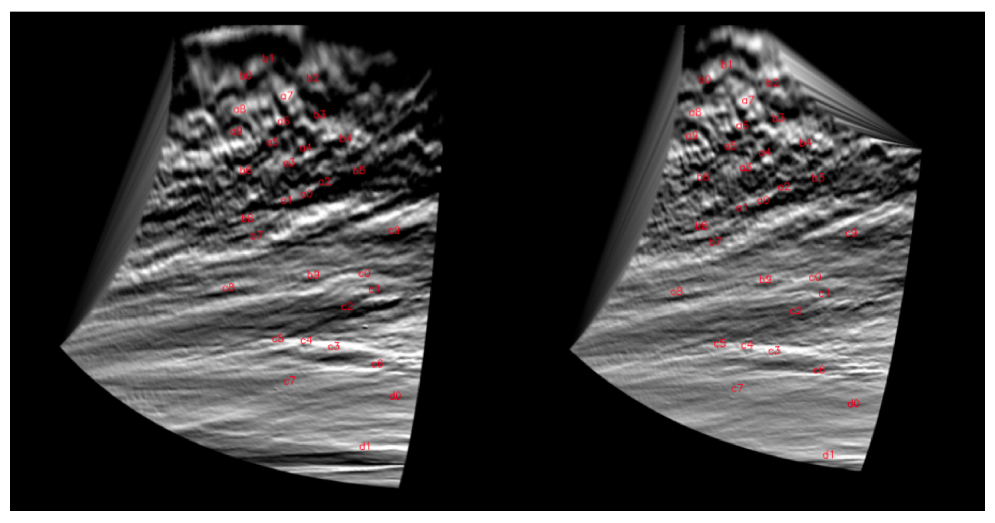
3.2. Cloud Tracking (CT) Wind Retrieval with VEx/VIRTIS-M

The long integration time needed to obtain a single VIRTIS data cube in the visible channel (∼12 min), along with the highly eccentric polar orbit of VEx with its apocenter located near south pole, limits VIRTIS-M observations (and cloud tracking) to the southern hemisphere. The spatial resolution in the images of these cubes vary between 45 km per pixel for high latitudes and about 15 km per pixel for lower latitudes. As a first step, the UV images from VIRTIS-M were processed and then projected onto equirectangular or polar coordinates (depending on the latitudinal coverage) with an angular resolution compatible with the worst spatial resolution for the images in the pair. The apparent motions of features observed in the images were measured manually, while pairs of images with a time separation of about 1 h were chosen. This time interval arose from the compromise and maximizing the precision of the speed measurements and ensuring that the shape of most of the cloud tracers remained coherent and clear for identification.

3.3. Cloud Tracking Method, Cloud Features Tracers, and Accuracy
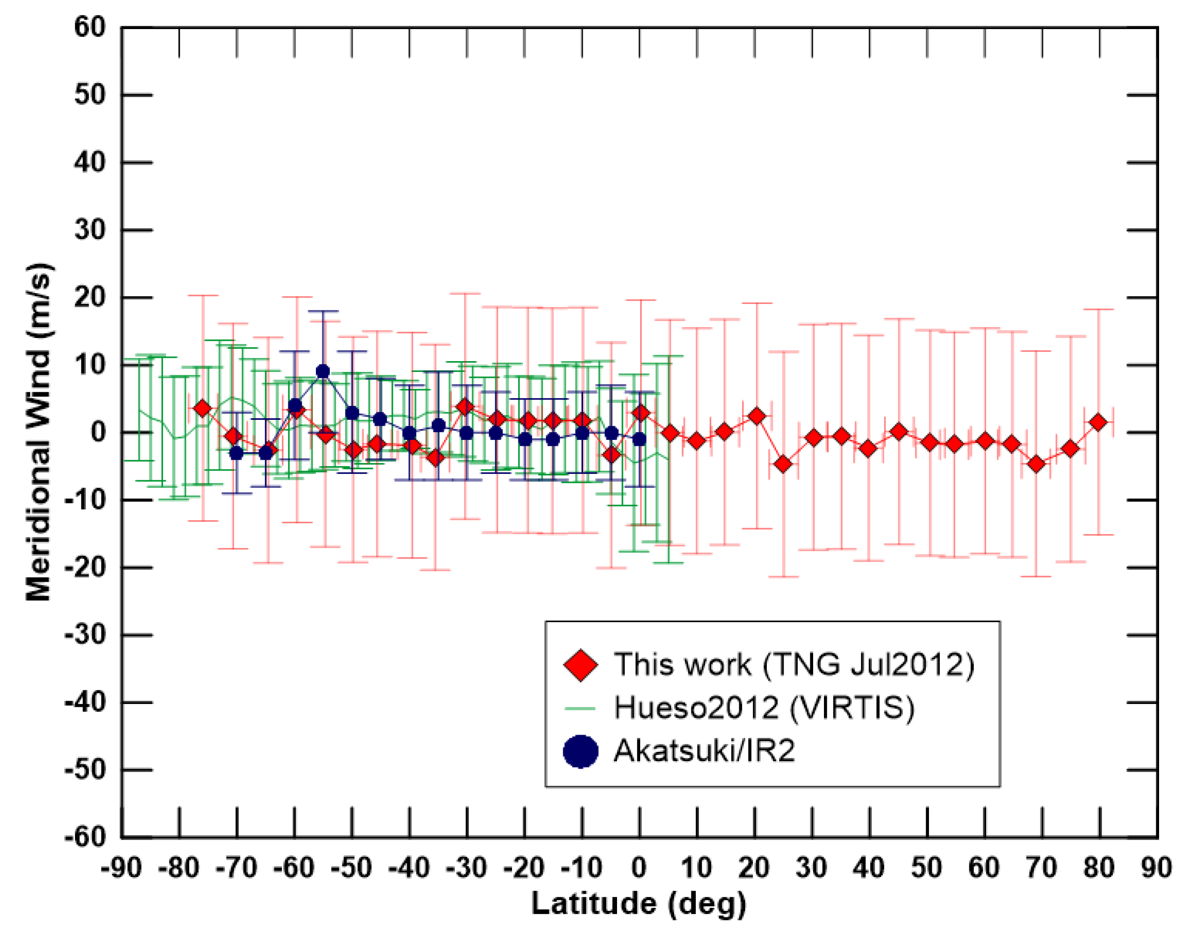
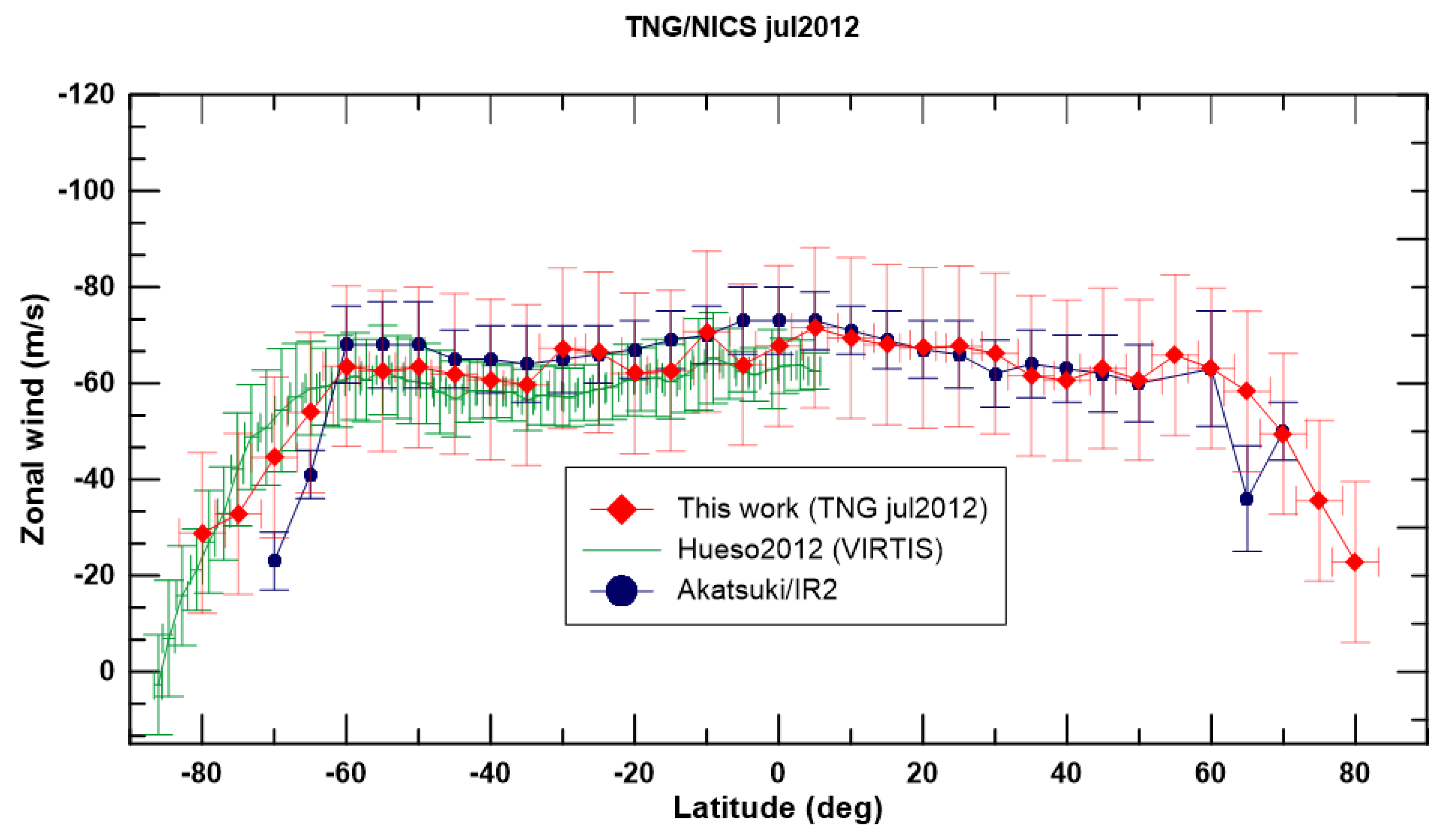
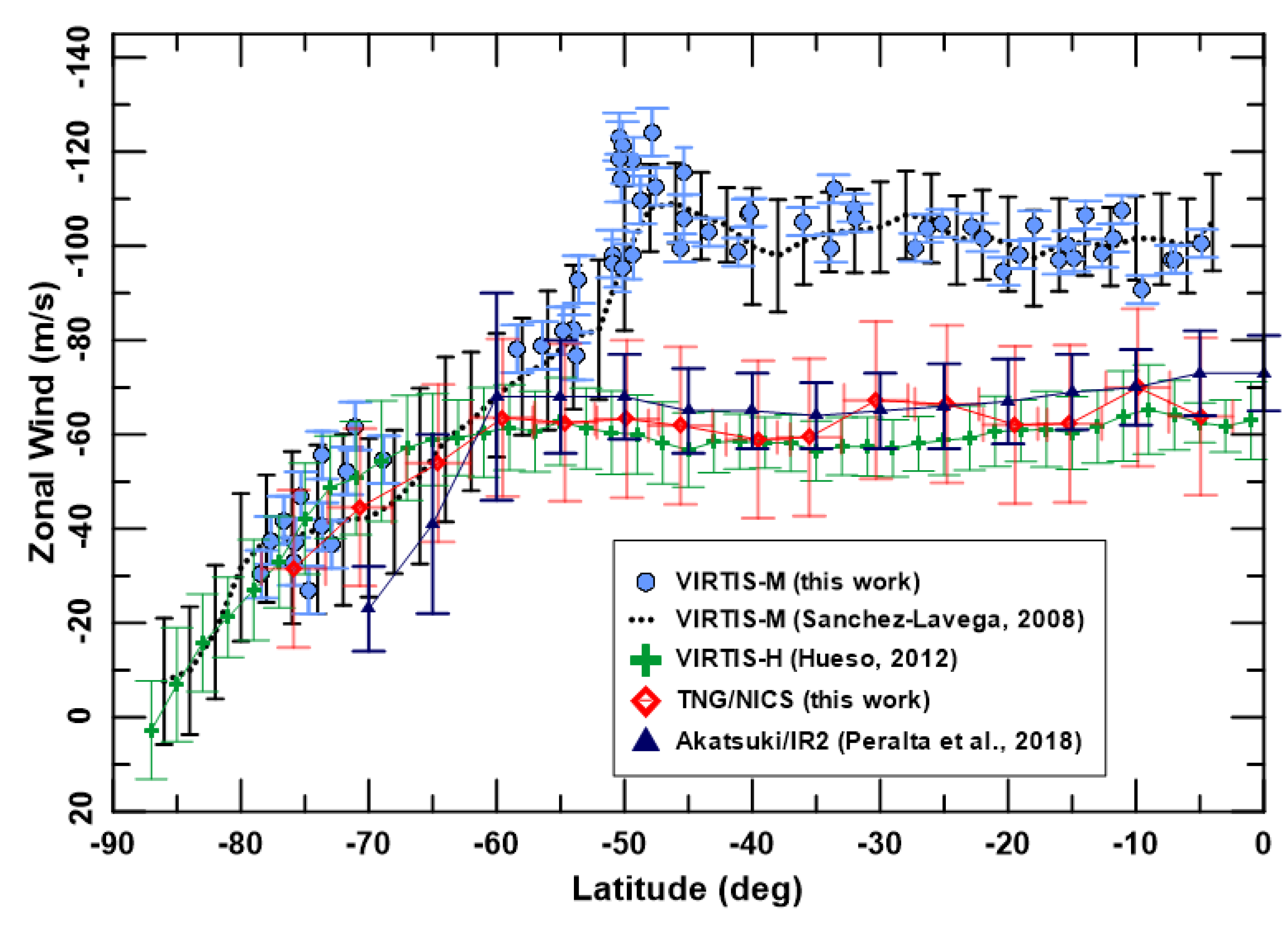
We used the same methodology as in Machado et al. [10,11], Gonçalves et al. [12], Peralta et al. [22] to retrieve the zonal and meridional winds in the VEx/VIRTIS-M and TNG/NICS images. We obtained cloud-tracked winds from VEx/VIRTIS-M following the temporal apparent motions of UV upper cloud features on Venus’ dayside (Venus/VIRTIS-M). A total of 72 cloud tracers from 2 pairs of dayside images, separated by a time interval of about 1 h (see Table 2), were identified to carry out the calculation of the wind velocities.
Concerning the near-infrared (1.74, 2.28 μ m), we used the same cloud tracking technique as for the VIRTIS-M UV (380 nm) images; although, the cloud patterns to be tracked on the nightside images keep some important differences. As mentioned before, on the dayside hemisphere, at visible/UV wavelengths, features can be distinguished as moving cloud patterns in the upper clouds, particularly thanks to the unknown UV absorber, which causes high-contrast patterns to form as solar radiation is absorbed and reflected back to the observer (VEx). On the nightside images at near-infrared wavelengths, the moving features we observe are formed by opacity patterns against the bright thermal emission from the deeper and warmer atmosphere, below the cloud layer.
To perform this method in the different dynamical regimes on both cloud layers, other factors should be considered as well. Previous nightside cloud tracking winds using space-based infrared images [5,21,22] have stated that the lower clouds at the bottom cloud deck, in contrast to the upper clouds, stay coherent for longer timescales (more than 2 h) and generally suffer less variability in the zonal wind speed [22]. For these reasons, the approximately one hour time interval (between images A and B) was perfectly suitable for our cloud tracking purposes when applied to TNG/NICS observations of the bottom cloud layer.
The following expressions were used for the calculation of the wind components:
u = ( a + H ) · cos λ · Δ ϕ Δ t · π 180
v = ( a + H ) · Δ λ Δ t · π 180
where u represents the zonal wind, v is the meridional wind component, a is the Venus radius, H is the height above the surface, ϕ and λ are the longitude and latitude in degrees, and Δ t is the time difference between the images (in seconds). Here, zonal wind means a horizontal (velocity vector along the same altitude) system of winds parallel to equator, while the meridional component represents winds in the north–south direction. The errors associated with both components of the cloud-tracked winds were calculated in the same way as in previous works [5,10,11,12,28]. Considering that the error in time δ t is quite small, the absolute errors for both components of the winds will be given by the following expressions, taken from the general forms described in Bevington et al. [45], i.e., δ u δ X / Δ t and δ v s . δ Y / Δ t , where δ X and δ Y are absolute errors for the spatial displacement of the clouds.
Concerning VEx/VIRTIS, the grids used for cloud tracking had a spatial resolution of 0 . 2 (for both latitudes and longitudes). Hence, δ X and δ Y were about 21 km, implying wind velocity measurements errors of ∼5 m·s 1 . Regarding ground-based TNG/NICS images, the grids used for cloud tracking purposes had a spatial resolution of 0 . 4 , and the retrieved zonal and meridional winds were affected by an error of about 30 m·s 1 .

4. Results

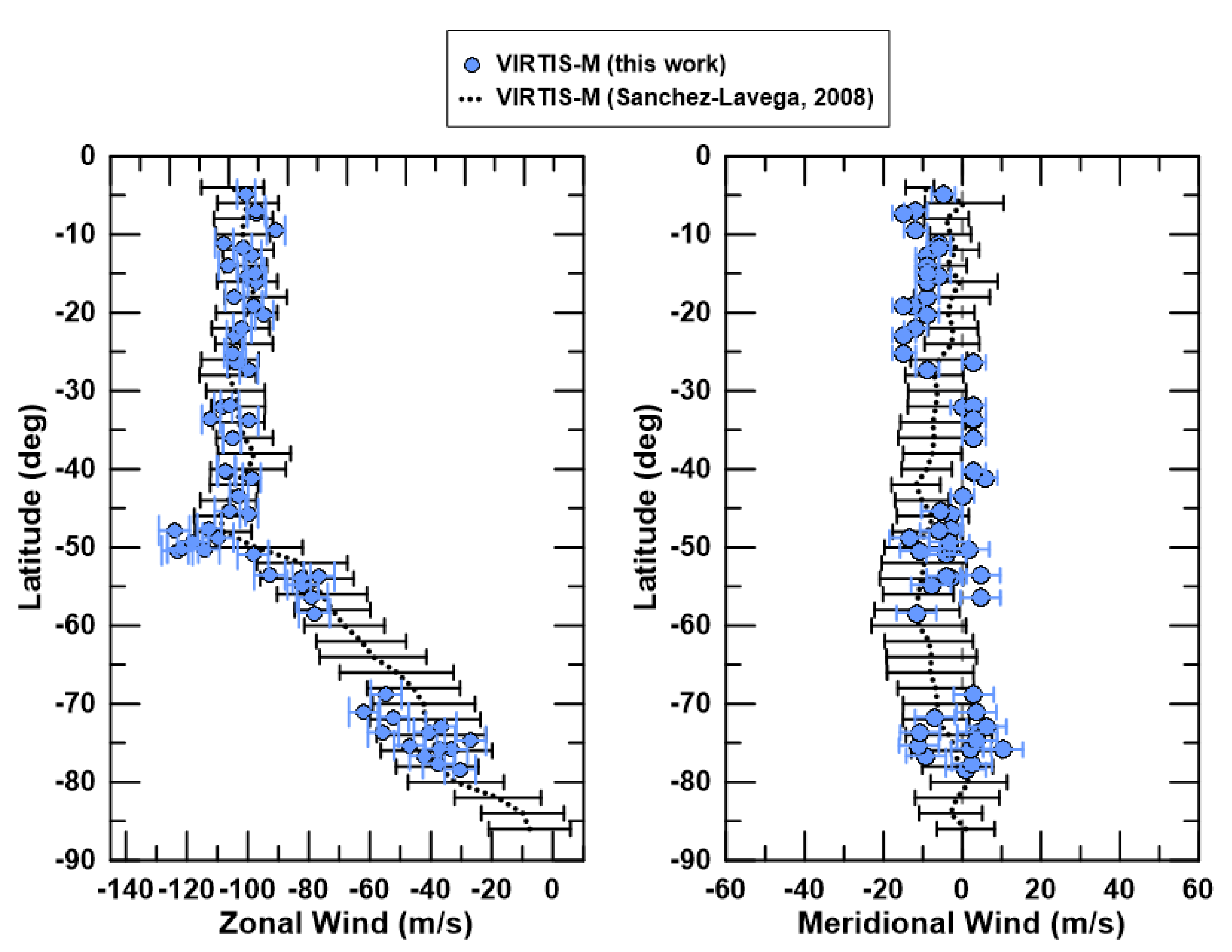
4.1. Winds at the Dayside Cloud Tops with VEx/VIRTIS-M

To perform cloud tracking with the VIRTIS-M images, we chose pairs of images separated by 60 min for the case of VEx orbit 2273, and about 45–60 min for orbit 2272. Sometimes we can observe noticeable differences between cloud patterns, these transiting from “patchy” to more “plain”, from lower to higher latitudes (see Figure 5).
Figure 6 shows our individual wind measurements along with the latitudinal profiles of zonally averaged speeds from Sanchez-Lavega et al. [5]. The results for the zonal component of the wind are displayed in the left graph, while the meridional component is shown on the right graph. The reference profiles from Sanchez-Lavega et al. [5] are based on cloud-tracked winds averaged along latitude bins of 2 , and the graphs exhibit the mean value and the corresponding standard deviation. One can note that, in both zonal and meridional latitudinal wind profiles, there is a gap in the covered latitudes (between 65 and 70 South). This was caused by the difficulty of finding reliable cloud tracers for this latitudinal region were cloud details were not easy to discern. Concerning the zonal wind (left side), we can note the presence of a nearly uniform zonal wind between the equator and about 45 S, where the zonal velocity of the wind is approximately constant with latitude. Around 50 S, a pronounced mid-latitude jet is apparent, a phenomenon already reported by Sanchez-Lavega et al. [5]. For higher latitudes, we observe a steady decrease in the zonal wind towards the pole. With respect to the meridional wind, results in Figure 6 (right side) exhibit no clear trend, discarding—at the time of the observations—net poleward circulation at the cloud tops. The results of a latitudinal wind profile (zonal and meridional winds), retrieved from Venus’ dayside space-based VEx/VIRTIS-M data at cloud tops level (around ∼70 km altitude) are in good agreement those from Sanchez-Lavega et al. [5], though the mid-latitude jet seems more enhanced than reported in other works.

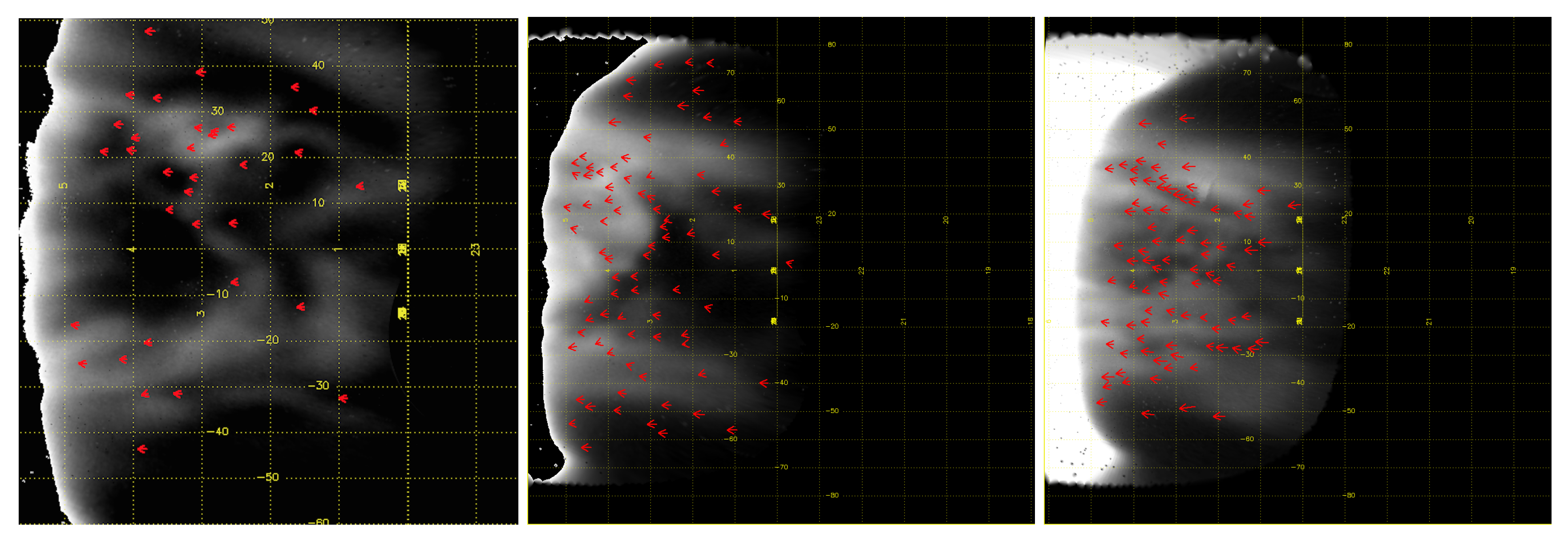
4.2. Cloud Patterns and Winds at the Nightside Lower Clouds with TNG/NICS

Due to the variable opacity of the deeper clouds, the infrared thermal radiation coming from the super-heated low atmosphere of Venus can be observed as high-contrasted markings at the lower clouds’ layer in the TNG/NICS images [17,18], with dark areas being related to thicker clouds (higher local opacity) and thin clouds seen as bright regions in the images since they allow the transmission of higher infrared thermal radiation fluxes coming from the hot lower atmosphere [13,18,21,46] (see Figure 7). We also studied the motions of these markings to retrieve wind velocity field on the nightside lower clouds of Venus [21,22].

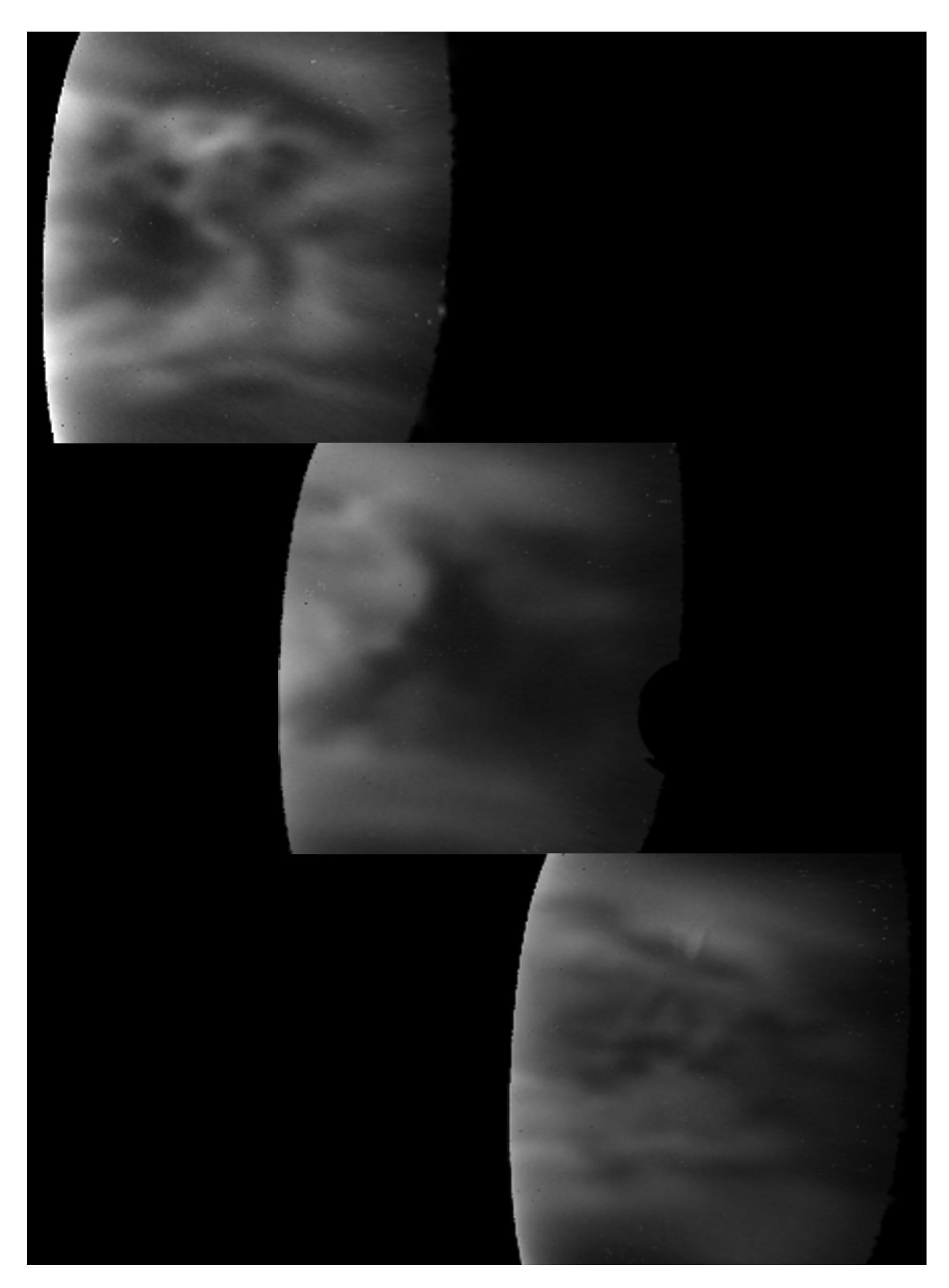
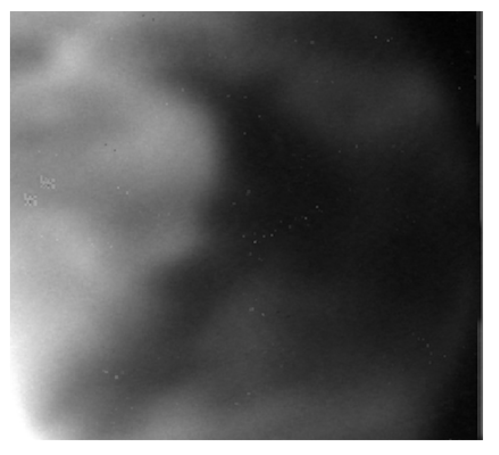
Morphology of the Nightside Lower Clouds with TNG/NICS Images

During the 3 consecutive days of our TNG/NICS observations, the morphology of the nightside lower clouds exhibited a huge diversity and fast variability (see Figure 7). Especially striking was how the morphology of the clouds changed from one day to the next, and the strong hemispherical asymmetries that were previously reported by Crisp et al. [14]. In our observations, the mid-latitude region is prone to show bright bands of clouds roughly aligned with the equator and hence correlated with the zonal wind. The limited spatial resolution of ground-based images prevents the visualization of many atmospheric phenomena identified in images from space missions, such as mesoscale waves, dark spots, mushroom-shaped clouds, vortexes, or patterns resembling shear instabilities [23,47,48,49]. Other features with larger scales, such as the sharp dark streaks, circumequatorial belts, or the bright equatorial wall, are infrequent [23], and they seemed missing during our TNG/NICS observations. The hemispherical symmetry observed for the bright mid-latitude bands during our observations and their orientation northwest-to-southeast (see Figure 7) suggests the manifestation of other large patterns, such as the bright planetary-scale streaks [50]; although, the limited spatial resolution of our images inhibits us from confirming whether these patterns are composed of thinner bright streaks [50].

4.3. Was the Planetary-Scale Cloud Discontinuity Present?

Peralta et al. [9] reported the astonishing discovery of a sharp equatorial discontinuity or “disruption” propagating at the middle and lower clouds of Venus, where no planetary wave had been identified before, except for mesoscale waves [23,51]. This discontinuity manifests as a dark band with cyclical behaviour that has remained recurrent for decades, rotating around the planet faster than the mean zonal flow. The related sharp cloud discontinuity spans along the mid-latitude region, almost at a planetary scale. Peralta et al. [9] suggests that this disruption may be the physical manifestation of a new type of Kelvin wave that propagates trapped about the equator, dissipates before arriving at the upper clouds, and significantly alters the spatial distribution of clouds’ aerosols [9].
In the present work, based on ground observations, the evidence of a planetary-scale homogeneous dark clouds is clear, such as an atmospheric wall (see Figure 8). This striking atmospheric feature was coherent with all the images we obtained for the second day of observations (12 July 2012). Nevertheless, it is not clear whether this event can be directly associated with a manifestation of the cloud discontinuity reported by Peralta et al. [9], since Kelvin waves are expected to propagate faster than the zonal mean flow. During 2016, Peralta et al. [9] estimated that the zonal phase speed of the discontinuity was, on average, 23 ± 9 m·s 1 faster than the mean zonal flow—a difference hard to detect given the accuracy of our wind speeds with TNG/NICS (∼30 m·s 1 ). In fact, no faster speeds were detected during 12 July 2012 (see Figure 9).

Dynamics of the Nightside Lower Clouds with TNG/NICS Images

Following the same method as Peralta et al. [29], we performed cloud tracking using phase correlation for template matching, being able to retrieve wind speeds that were comparable with some cases measurements from space orbiters (see Figure 9). A set of cloud patterns were selected attending to their shape coherence along time and they were tracked along time to characterize their motions and, therefore, the wind speeds (see in Figure 10). For each one of the three days of observations, we retrieved the velocity based on each pair of related tracers (from image A to B). We measured both horizontal components (zonal and meridional) of the wind.
For the zonal component of the wind, we built a latitudinal profile of zonally averaged velocity values in latitude bins of 5 for each day of observations (see Figure 9). The error bars associated with each velocity were derived from the calculations described in Section 3.3. These were a direct consequence of the observing conditions, mainly from the images’ resolution and the time interval between the exposures that produced images A and B. They also correspond to the standard deviation, related to the set of wind velocities retrieved within each latitude bin.
In Figure 9, one can clearly see that equatorward of 60 , the zonal wind is around 60 m·s 1 in both hemispheres, with a variability ranging 5–10 m·s 1 . Near the 60 latitude, in both hemispheres, there are hints of a weak jet, although this cannot confirmed out of the error bars. At higher latitudes, we observed the expected steady decrease towards the poles already reported in previous works [5,21,22,52].
In relation to the meridional flow of the wind, despite covering a wide range of latitudes and local time positions, the accuracy of our velocity measurements prevents us from discerning any clear trend in the zonally averaged profile out of the error bars (see Figure 11), consistent with previous reports from VEx [21] and Akatsuki [22].
The results concerning the zonal component of the wind velocity at the lower cloud deck of Venus is undoubtedly a major result from this analysis, given past measurements with ground-based observations [17,18,22]. We can see, in Figure 12, a consolidated latitudinal profile of the zonal wind from all cloud-tracked measurements from all days of our TNG/NICS observational run. The retrieved zonal winds have the particularity that they were measured with an improved cloud tracking method that uses phase correlation between images. In Figure 12, we can note the high consistency between previous space-based (VEx/VIRTIS) zonal wind latitudinal profile from Hueso et al. [21] and Peralta et al. [22] (Akatsuki/IR2) at lower cloud deck of Venus, and the latitudinal zonal wind velocity profile coming from ground-based observations in this study (TNG/NICS); although, in this study, the presence of an equatorial jet is not evident.

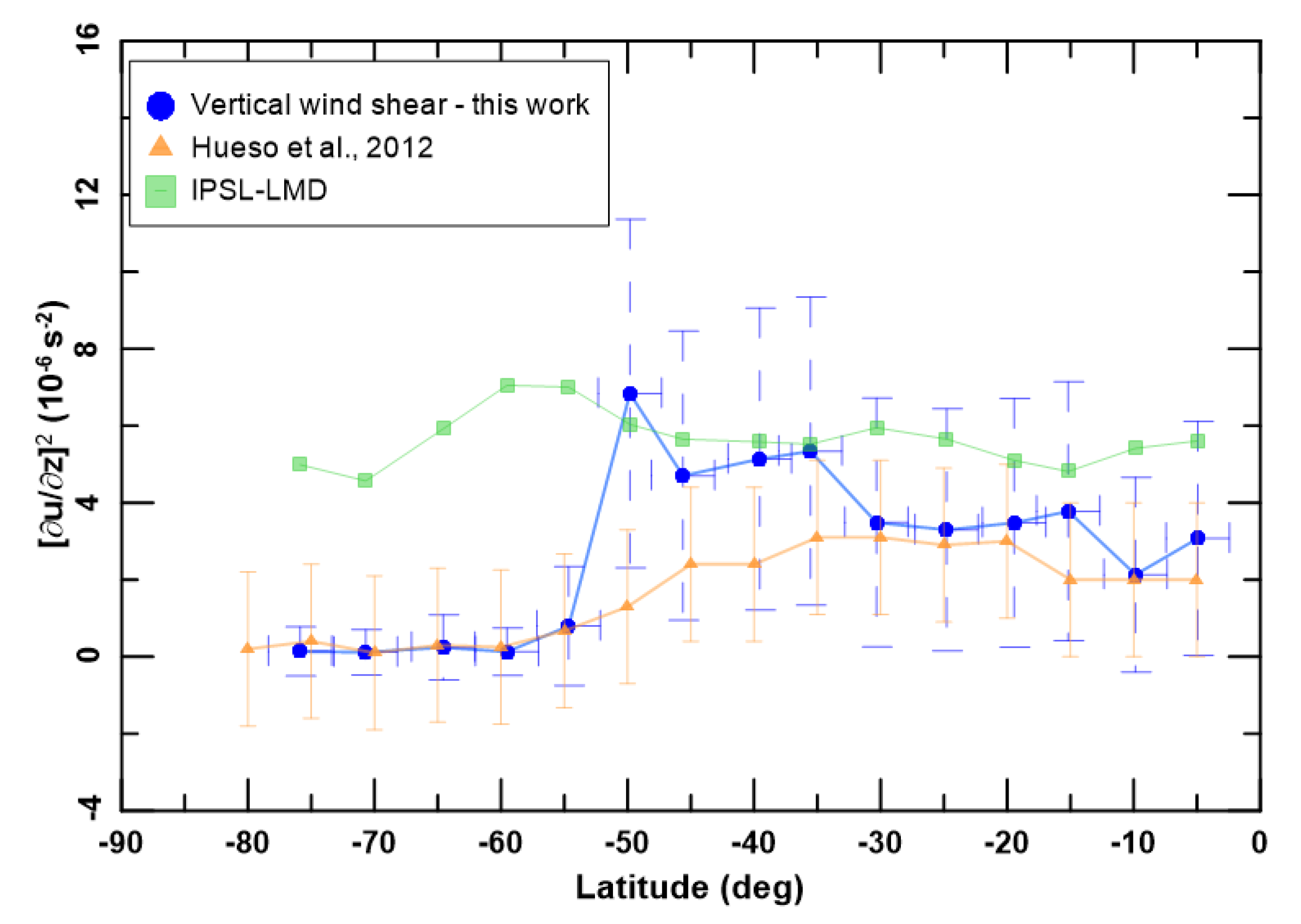
5. Discussion and Conclusions

The ground-based data obtained with TNG/NICS during 11–13 of July 2012 have allowed us to monitor the wind variability on the nightside lower cloud deck of Venus. The latitudinal zonal wind profile obtained from our ground-based observations are consistent with previous space-based results. Given that, from the Earth, it is possible to observe both hemispheres of Venus simultaneously, our observations helped us to extend the monitoring of deeper winds at the northern hemisphere with a quality closer to the observations by Akatsuki/IR2 [22], and drastically improve past ground-based observations [16,17], confirming zonal winds that can be regarded as hemispherically symmetric in contrast to the cloud morphology. Our measurements during 11–13 July 2012 also discard the presence of the equatorial jets reported during 2016 with Akatsuki/IR2 data [22,48].
As already stated, our measurements of the nightside meridional winds display no clear trend at the lower cloud deck, a result in agreement with previous reports from VEx [21] and Akatsuki [22]. Nevertheless, using higher-accuracy wind measurements and the larger data set from VIRTIS-M, Gorinov et al. [52] showed that meridional winds at the nightside lower clouds exhibit abrupt changes in its sign at lower latitudes, a result to be confirmed with our further studies via more accurate measurements. In any case, results of meridional wind velocities from both ground-based observations and space missions (VEx/VIRTIS and Akatsuki/IR2) [21,22,52] seem inconsistent with a Hadley cell circulation at the lower clouds.
We detected a significant variability in the opacity of lower clouds’ morphology along the different days of observations (see Figure 1 and Figure 7), a phenomenon already reported in previous works [16,22]. Even though the cloud pattern visible in the TNG/NICS images during 12 July 2012 (see Figure 8) can be attributed to the cloud discontinuity reported by Peralta et al. [9], caution must be taken since its associated zonal speeds do not seem faster than the background zonal flow above the error bars.
The dayside cloud-tracked winds obtained based on VIRTIS-M, reported in this work, are consistent with previous results (from Sanchez-Lavega et al. [5] and with local time averaged zonal wind profiles from Horinouchi et al. [8]). The zonal wind retrieved at mid-latitudes cloud tops indicates an almost homogeneous flow of the zonal wind (around 100 m·s 1 ), with a steep decrease at the latitudes where it is expected to find the so-called cold collar (nearly 60 S). Figure 13 shows two levels of the atmosphere of Venus sounded in the framework of the coordinated observations undertaken in this project. We can see the averaged zonal velocities of dayside cloud tops ranging around 100 m·s 1 in the mid-latitudes region with a steep decrease for higher latitudes. However, the nightside NIR observations sensing the lower clouds present an almost steady zonal wind profile of the order of 60 m·s 1 , again in the mid-latitude region with a rapid decrease at higher latitudes. The results obtained are consistent with the expected increase in the zonal wind speed from lower layers of the atmosphere to the cloud top altitude.
The coordinated observations between Venus nightside lower cloud layer with TNG/ NICS (ground-based), and VEx/VIRTIS-M dayside cloud tops observations allowed us to compare the dynamics of Venus simultaneously at the two different atmospheric altitude levels of the lower clouds and top of the upper clouds. This made it possible to also have an integrated view of the atmospheric dynamics of Venus in the dayside and nightside of the planet, since in situ wind measurements by space missions indicate that the zonal wind speeds at the deeper clouds are similar on the day and night sides: Pioneer Venus Day and Night probes exhibited zonal speeds discrepancies below 7 m·s 1 within altitudes ranging 50–60 km [40], while VEGA balloons (propagating along a similar range of altitudes from the night to the dayside) generally displayed, for the zonal speeds, Doppler residuals below 4 m·s 1 , with a maximum of 16 m·s 1 [53]. This similarity between the deeper winds at the day and night sides are also supported by numerical simulations [30]. The new modelling tool, the Venus Climate Database (VCD), from 2021 [4,54], also highly suggests in its simulations and predictions that the zonal wind at the bottom cloud level on the atmosphere of Venus is stable along all planetary local times. Therefore, we can consider that the zonally averaged profile of zonal winds at the nightside lower clouds is also representative of their dayside counterpart, and our results for the wind speeds at the upper (VIRTIS-M) and lower clouds (NICS) can be combined to estimate the vertical shear of the zonal wind on the dayside of Venus.
If we consider that the lower clouds are located within altitudes ∼48–55 km [29] and the top of the upper clouds within ∼70–74 km [42], their vertical separation to be roughly estimated to be 20 ± 4 km. Figure 14 displays our estimation of the vertical shear of the zonal wind between these two atmospheric layers, compared with the same type of profile estimated with only VIRTIS-M by Hueso et al. [21]. Note that these values of the vertical shear cannot be representative for the real vertical distribution of the shear, since the largest values (higher than mean values represented here) are concentrated between the upper and bottom of the upper clouds (60–70 km) [21]. Figure 14 shows that our estimations of ( u / z ) 2 during 11–13 July 2012 are consistent with those obtained by Hueso et al. [21] with VEx/VIRTIS-M data during the years 2006–2008. Some discrepancy shown at about 50 of latitude could be a consequence of the notorious mid-latitudes jet measured by us at the top of the clouds, which appears smoother on the results from Hueso et al. [21], perhaps due to the longer time interval that produced their averaged winds and to the known temporal variability of the mid-latitudes’ jets, so the observed differences may be attributed to the amount of data and time coverage used in each case. Regarding the comparison with the IPSL-VGCM (LMD) modelling profile, [55,56], it is notorious that the predicted vertical wind shear profile shows consistency with the observation-based profile between mid-latitudes; however, for higher latitudes (higher than the location of the so-called cold collar), there is some lack of agreement between observations and the prediction profile—this was already pointed out by Machado et al. [27] for the case of zonal wind comparison, due to a decrease in the winds’ velocity at higher latitudes than in the observations’ profile.
Regarding the behaviour with latitude, both profiles of ( u / z ) 2 exhibit a gradual increase from equator to mid-latitudes, followed by a steeper decrease up to about 60 S. The lower values for ( u / z ) 2 at higher latitudes are expected since the difference between zonal speeds at distinct cloud layers becomes smaller when winds decrease towards to the poles [5,21,28,42]. Furthermore, the highest value for ( u / z ) 2 occurs at ∼50 S, close to the edge of the cold collar and a region where vertical instabilities cloud be favoured [28].
In this work, we used an improved cloud tracking method based on a phase correlation between images. We also improved the accuracy of the latitudes and longitudes assignment (i.e., navigation) to the tracers marked on the ground-based images in order to optimize the determination of shifts in cloud features between images. The attributed coordinates to each tracer came from the precise navigation of telescope images by the use of SPICE kernels; in this manner, each image pixel benefited from an accurate navigation process, which increased the precision of the retrieved wind velocities.
Ground-based infrared observations allied to the evolved cloud tracking method used in this work comprise an effective tool to explore and study the lower cloud deck of Venus. Ground-based observations obtained with telescopes and infrared detectors, in Earth’s atmospheric infrared transparency windows, constitute a complementary and competitive technique for studying the atmosphere dynamics of the lower cloud layer on the nightside of Venus.
In order to enhance the spatial resolution and accuracy of retrieval of wind velocity, we intend to consider using deep machine learning methods applied to ground-based observations of extended sources. This method has recently been used with success in the context of solar investigations by Baso et al. [57], Xiangchun et al. [58], Dash et al. [59].
However, adaptive optics is also a prospect to consider in future observations in order to better compensate for atmospheric turbulence. A technique, also coming from solar physics, was successfully used in obtaining a homogeneous seeing improvement over a wide field by Schmidt et al. [60]. The adaptation of this recent method also opens a window to future improvements in studies of the atmosphere of Venus based upon ground-based observations.

Author Contributions

Conceptualization, P.M. and J.P.; data curation, P.M., J.P., J.E.S., F.B. and R.G.; formal analysis, P.M., J.P., J.E.S., and F.B.; investigation, P.M. and J.P.; methodology, P.M. and J.P.; resources, F.B. and M.S.; software, J.P.; supervision, P.M. and J.P.; validation, P.M. and J.P.; visualization, J.E.S., F.B., M.S. and R.G.; writing—original draft, P.M. and J.P.; writing—review and editing, J.P., P.M., J.E.S., F.B. and R.G. All authors have read and agreed to the published version of the manuscript.

Funding

This research was funded by the Portuguese Fundação Para a Ciência e Tecnologia under project P-TUGA Ref. PTDC/FIS-AST/29942/2017 through national funds and by FEDER through COMPETE 2020 (Ref. POCI-01-0145 FEDER-007672). It was also funded by JAXA’s Top Young Fellowship (ITYF) and EMERGIA program granted by Junta de Andalucía (Spain).

Data Availability Statement

Data available in a publicly accessible repository. The data presented in this study are openly available in “Machado, Pedro (2021)”, Venus’ cloud-tracked winds using ground and space based observations with TNG/NICS and VEx/VIRTIS, Mendeley Data, V1, doi: 10.17632/sbkw5g579t.1.

Acknowledgments

We credit the European Space Agency, and the associated funding bodies Centre National d’Etudes Spatiales (France) and Agenzia Spaziale Italiana (Italy), as well as the VIRTIS PIs, Giuseppe Piccioni (IASF-INAF), and Pierre Drossart (LESIA) for providing the VIRTIS-M data. We acknowledge support from the Portuguese Fundação Para a Ciência e a Tecnologia (ref. PD/BD/128019/2016 (R.G.), 2021.05455.BD (F.B.) and project P-TUGA ref. PTDC/FIS-AST/29942/2017 (P.M., J.P., R.G., F.B., and M.S.)) through national funds and by FEDER through COMPETE 2020 (ref. POCI-01-0145 FEDER-007672). J.E.S. acknowledges support from the University of Lisbon through the BD2017, program approved by law 89/2014. Javier Peralta acknowledges funding from JAXA’s International Top Young Fellowship (ITYF2014) and EMERGIA20_00414 by Junta de Andalucía (Spain). We gratefully acknowledge the collaboration of the TNG staff at La Palma (Canary Islands, Spain)—the observations were made with the Italian Telescopio Nazionale Galileo (TNG) operated on the island of La Palma by the Fundacion Galileo Galilei of the INAF (Istituto Nazionale di Astrofisica) at the Spanish Observatorio del Roque de los Muchachos of the Instituto de Astrofisica de Canarias.

Conflicts of Interest

The authors declare no conflict of interest.

References

  1. Mueller, N.T.; Helbert, J.; Erard, S.; Piccioni, G.; Drossart, P. Rotation period of Venus estimated from Venus Express VIRTIS images and Magellan altimetry. Icarus 2011, 217, 474–483. [Google Scholar] [CrossRef] [Green Version]
  2. Ignatiev, N.I.; Titov, D.V.; Piccioni, G.; Drossart, P.; Markiewicz, W.J.; Cottini, V.; Manoel, N. Altimetry of the Venus cloud tops from the Venus Express observations. J. Geophys. Res. 2009, 114, E00B43. [Google Scholar] [CrossRef]
  3. Titov, D.V.; Ignatiev, N.I.; McGouldrick, K.; Wilquet, V.; Wilson, C.F. Clouds and Hazes of Venus. Space Sci. Rev. 2018, 214, 126. [Google Scholar] [CrossRef] [Green Version]
  4. Lebonnois, S.; Hourdin, F.; Eymet, V.; Crespin, A.; Fournier, R.; Forget, F. Superrotation of Venus’ atmosphere analyzed with a full general circulation model. J. Geophys. Res. 2010, 115, E06006. [Google Scholar] [CrossRef]
  5. Sanchez-Lavega, A.; Hueso, R.; Piccioni, G.; Drossart, P.; Peralta, J.; Perez-Hoyos, S.; Lebonnois, S. Variable winds on Venus mapped in three dimensions. Geophys. Res. Lett. 2008, 35, L13204. [Google Scholar] [CrossRef] [Green Version]
  6. Nakamura, M.; Imamura, T.; Ishii, N.; Abe, T.; Kawakatsu, Y.; Hirose, C.; Kamata, Y. AKATSUKI returns to Venus. Earth Planets Space 2016, 68, 201668. [Google Scholar] [CrossRef] [Green Version]
  7. Fukuhara, T.; Futaguchi, M.; Hashimoto, G.L.; Horinouchi, T.; Imamura, T.; Iwagaimi, N.; Kouyama, T.; Murakami, S.-Y.; Nakamura, M.; Ogohara, K.; et al. Large stationary gravity wave in the atmosphere of Venus. Nat. Geosci. 2017, 10, 85–88. [Google Scholar] [CrossRef]
  8. Horinouchi, T.; Kouyama, T.; Lee, Y.J.; Murakami, S.; Ogohara, K.; Takagi, M.; Imamura, T.; Nakajima, K.; Peralta, J.; Yamazaki, A. Mean winds at the cloud top of Venus obtained from two wavelength UV imaging by Akatsuki. Earth Planets Space 2018, 70, 10. [Google Scholar] [CrossRef]
  9. Peralta, J.; Navarro, T.; Vun, C.W.; Sánchez-Lavega, A.; McGouldrick, K.; Horinouchi, T.; Imamura, T.; Hueso, R.; Boyd, J.P.; Schubert, G.; et al. A long-lived sharp disruption on the lower clouds of Venus. Geophys. Res. Lett. 2020, 42, 705–711. [Google Scholar] [CrossRef]
  10. Machado, P.; Widemann, T.; Luz, D.; Peralta, J. Wind circulation regimes at Venus’ cloud tops: Ground-based Doppler velocimetry using CFHT/ESPaDOnS and comparison with simultaneous cloud tracking measurements using VEx/VIRTIS in February 2011. Icarus 2014, 243, 249–263. [Google Scholar] [CrossRef]
  11. Machado, P.; Widemann, T.; Peralta, J.; Gonçalves, R.; Donati, J.; Luz, D. Venus cloud-tracked and doppler velocimetry winds from CFHT/ESPaDOnS and Venus Express/VIRTIS in April 2014. Icarus 2017, 285, 8–26. [Google Scholar] [CrossRef]
  12. Gonçalves, R.; Machado, P.; Widemann, T.; Peralta, J.; Watanabe, S.; Yamazaki, A.; Silva, J. Venus’ cloud top wind study: Coordinated Akatsuki/UVI with cloud tracking and TNG/HARPS-N with Doppler velocimetry observations. Icarus 2020, 335, 113418. [Google Scholar] [CrossRef]
  13. Allen, D.A.; Crawford, J.W. Cloud structure on the dark side of Venus. Nature 1984, 307, 222–224. [Google Scholar] [CrossRef]
  14. Crisp, D.; Sinton, W.M.; Hodapp, K.W.; Ragent, B.; Gerbault, F.; Goebel, J.H.; Probst, R.G.; Allen, D.A.; Pierce, K.; Stapelfeldt, K.R. The Nature of the Near-Infrared Features on the Venus Night Side. Science 1989, 246, 506–509. [Google Scholar] [CrossRef] [PubMed]
  15. Chanover, N.J.; Glenar, D.A.; Hillman, J.J. Multispectral near-IR imaging of Venus nightside cloud features. J. Geophys. Res. 1998, 103, 31335. [Google Scholar] [CrossRef]
  16. Crisp, D.; McMuldroch, S.; Stephens, S.K.; Sinton, W.M.; Ragent, B.; Hodapp, K.W.; Probst, R.G.; Doyle, L.R.; Allen, D.A.; Elias, J. Ground-Based Near-Infrared Imaging Observations of Venus during the Galileo Encounter. Science 1991, 253, 1538. [Google Scholar] [CrossRef]
  17. Limaye, S.S.; Warell, J.; Bhatt, B.C.; Fry, P.M.; Young, E. Multi-observatory observations of night-side of Venus at 2.3 micron—Atmospheric circulation from tracking of cloud features. Bull. Astron. Soc. India 2006, 34, 189–201. [Google Scholar]
  18. Tavenner, T.; Young, E.F.; Bullock, M.A.; Murphy, J. Global mean cloud coverage on Venus in the near-infrared. Planet Space Sci. 2008, 56, 1435–1443. [Google Scholar] [CrossRef]
  19. Carlson, R.W.; Baines, K.H.; Encrenaz, T.; Taylor, F.W.; Drossart, P.; Kamp, L.W.; Pollack, J.B.; Lellouch, E.; Collard, A.D.; Calcutt, S.B.; et al. Galileo infrared imaging spectroscopy measurements at Venus. Science 1991, 253, 1541–1548. [Google Scholar] [CrossRef]
  20. Hueso, R.; Sánchez-Lavega, A.; Piccioni, G.; Drossart, P.; Gérard, J.C.; Khatuntsev, I.; Zasova, L.; Migliorini, A. Morphology and dynamics of Venus oxygen airglow from Venus Express/visible and infrared thermal imaging spectrometer observations. J. Geophys. Res. Planets 2008, 113. [Google Scholar] [CrossRef] [Green Version]
  21. Hueso, R.; Peralta, J.; Sanchez-Lavega, A. Assessing the long-term variability of Venus winds at cloud level from VIRTIS-Venus Express. Icarus 2012, 217, 585–598. [Google Scholar] [CrossRef]
  22. Peralta, J.; Muto, K.; Hueso, R.; Horinouchi, T.; Sánchez-Lavega, A.; Murakami, S.Y.; Luz, D. Nightside Winds at the Lower Clouds of Venus with Akatsuki/IR2: Longitudinal, Local Time, and Decadal Variations from Comparison with Previous Measurements. Astrophys. J. Suppl. Ser. 2018, 239, 29. [Google Scholar] [CrossRef] [Green Version]
  23. Peralta, J.; Sánchez-Lavega, A.; Horinouchi, T.; McGouldrick, K.; Garate-Lopez, I.; Young, E.F.; Bullock, M.A.; Lee, Y.J.; Imamura, T.; Satoh, T.; et al. New cloud morphologies discovered on the Venus’s night during Akatsuki. Icarus 2019, 333, 177–182. [Google Scholar] [CrossRef]
  24. Iwagami, N.; Sakanoi, T.; Hashimoto, G.L.; Sawai, K.; Ohtsuki, S.; Takagi, S.; Takagi, K.; Ueno, M.; Kameda, S.; Murakami, S.-Y.; et al. Initial products of Akatsuki 1-μm camera. Earth Planets Space 2018, 70, 6. [Google Scholar] [CrossRef] [Green Version]
  25. Acton, C.; Bachman, N.; Semenov, B.; Wright, E. A look towards the future in the handling of space science mission geometry. Planet Space Sci. 2018, 150, 9–12. [Google Scholar] [CrossRef]
  26. Drossart, P.; Piccioni, G.; Gérard, J.C.; Lopez-Valverde, M.A.; Sanchez-Lavega, A.; Zasova, L.; Hueso, R.; Taylor, F.W.; Bézard, B.; Adriani, A.; et al. A dynamic upper atmosphere of Venus as revealed by VIRTIS on Venus Express. Nature 2007, 450, 641–645. [Google Scholar] [CrossRef]
  27. Machado, P.; Widemann, T.; Peralta, J.; Gilli, G.; Espadinha, D.; Silva, J.E.; Brasil, F.; Ribeiro, J.; Goncalves, R. Venus Atmospheric Dynamics at Two Altitudes: Akatsuki and Venus Express Cloud Tracking, Ground-Based Doppler Observations and Comparison with Modelling. Atmosphere 2021, 12, 506. [Google Scholar] [CrossRef]
  28. Peralta, J.; Hueso, R.; Sánchez-Lavega, A. A reanalysis of Venus winds at two cloud levels from Galileo SSI images. Icarus 2007, 190, 469–477. [Google Scholar] [CrossRef]
  29. Peralta, J.; Lee, Y.J.; Hueso, R.; Clancy, R.T.; Sandor, B.; Sànchez-Lavega, A.; Imamura, T.; Omino, M.; Machado, P.; Lellouch, E.; et al. The Winds of Venus during the Messenger’s Flyby. Geophys. Res. Lett. 2017, 44, 3907–3915. [Google Scholar] [CrossRef]
  30. Garate-Lopez, I.; Lebonnois, S. Latitudinal Variation of Clouds’ Structure Responsible for Venus’ Cold Collar. Icarus 2018, 314, 1–11. [Google Scholar] [CrossRef] [Green Version]
  31. Venus Coordinated Campaign Transit of Venus. 2012. Available online: https://lesia.obspm.fr/venus-atm-wiki/index.php/Venus_coordinated_campaign_Transit_of_Venus (accessed on 18 December 2021).
  32. Farsiu, S.; Robinson, M.D.; Elad, M.; Milanfar, P. Fast and robust multiframe super resolution. IEEE Trans. Image Process. 2004, 13, 1327–1344. [Google Scholar] [CrossRef] [PubMed]
  33. Mendikoa, I.; Sánchez-Lavega, A.; Pérez-Hoyos, S.; Hueso, R.; Rojas, J.F.; Aceituno, J.; Aceituno, F.; Murga, G.; De Bilbao, L.; García-Melendo, E. PlanetCam UPV/EHU: A Two-channel Lucky Imaging Camera for Solar System Studies in the Spectral Range 0.38–1.7 μm. Astron. Instrum. Telesc. Obs. Site Charact. 2016, 128, 035002. [Google Scholar] [CrossRef] [Green Version]
  34. Sanchez-Lavega, A.; Peralta, J.; Gomez-Forrellad, J.M.; Hueso, R.; Pérez-Hoyos, S.; Mendikoa, I.; Rojas, J.F.; Horinouchi, T.; Lee, Y.J.; Watanabe, S. Venus Cloud Morphology and Motions from Ground-Based Images at the Time of the Akatsuki Orbit Insertion. Astrophys. J. Lett. 2016, 833, L7. [Google Scholar] [CrossRef] [Green Version]
  35. Mackay, C.D.; Baldwin, J.; Law, N.; Warner, P. High-resolution imaging in the visible from the ground without adaptive optics: New techniques and results. In Proceedings Ground-Based Instrumentation for Astronomy; SPIE Astronomical Telescopes + Instrumentation: Glasgow, UK, 2004; Volume 5492. [Google Scholar] [CrossRef]
  36. Lodieu, N.; Zapatero Osorio, M.R.; Martín, E.L. Lucky Imaging of M subdwarfs. Astron. Astrophys. 2009, 499, 729–736. [Google Scholar] [CrossRef] [Green Version]
  37. Gallaway, M. An Introduction to Observational Astrophysics; Springer: New York, NY, USA, 2020. [Google Scholar]
  38. Hueso, R.; Legarreta, J.; Rojas, J.F.; Peralta, J.; Pérez-Hoyos, S.; Del Río-Gaztelurrutia, T.; Sánchez-Lavega, A. The Planetary Laboratory for Image Analysis (PLIA). Adv. Space Res. 2010, 46, 1120–1138. [Google Scholar] [CrossRef]
  39. Cardesín, A. Study and Implementation of the End-to-End Data Pipeline for the VIRTIS Imaging Spectrometer on Board Venus Express: From Science Operation Planning to Data Archiving and Higher Level Processing. Ph.D. Thesis, Centro Interdipartimentale di Studi e Attività Spaziali (CISAS), Universita degli Studi di Padova, Padova, Italy, January 2010. [Google Scholar]
  40. Sánchez-Lavega, A.; Lebonnois, S.; Imamura, T.; Read, P.; Luz, D. The Atmospheric Dynamics of Venus. Space Sci. Rev. 2017, 212, 1541–1616. [Google Scholar] [CrossRef]
  41. Khatuntsev, I.; Patsaeva, M.; Titov, D.; Ignatiev, N.; Turin, A.; Limaye, S.; Markiewicz, W.; Almeida, M.; Roatsch, T.; Moissl, R. Cloud level winds from the Venus Express Monitoring Camera imaging. Icarus 2013, 226, 140–158. [Google Scholar] [CrossRef]
  42. Hueso, R.; Peralta, J.; Garate-Lopez, I.; Bados, T.V.; Sanchez-Lavega, A. Six years of Venus winds at the upper cloud level from UV, visible and near-infrared observations from VIRTIS on Venus Express. Planet Space Sci. 2015, 113–114, 78–99. [Google Scholar] [CrossRef]
  43. Peralta, J.; Iwagami, N.; Sánchez-Lavega, A.; Lee, Y.J.; Hueso, R.; Narita, M.; Imamura, T.; Miles, P.; Wesley, A.; Kardasis, E.; et al. Morphology and Dynamics of Venus’s Middle Clouds with Akatsuki/IR1. Geophys. Res. Lett. 2019, 46, 2399–2407. [Google Scholar] [CrossRef] [Green Version]
  44. Acton, C.H. Ancillary Data Services of NASA’s Navigation and Ancillary Information Facility. Planet Space Sci. 1996, 44, 65–70. [Google Scholar] [CrossRef]
  45. Bevington, P.R.; Robinson, D.K. Data Reduction and Error Analysis for the Physical Sciences, 2nd ed.; McGraw-Hill: New York, NY, USA, 1992. [Google Scholar]
  46. McGouldrick, K.; Momary, T.W.; Baines, K.H.; Grinspoon, D.H. Quantication of middle and lower cloud variability and mesoscale dynamics from Venus Express/VIRTIS observations at 1.74 microns. Icarus 2012, 217, 615–628. [Google Scholar] [CrossRef]
  47. Satoh, T.; Sato, T.M.; Nakamura, M.; Kasaba, Y.; Ueno, M.; Suzuki, M.; Ohtsuki, S. Performance of Akatsuki/IR2 in Venus orbit: The first year. Earth Planets Space 2017, 69, 154. [Google Scholar] [CrossRef] [Green Version]
  48. Horinouchi, T.; Murakami, S.; Satoh, T.; Peralta, J.; Ogohara, K.; Kouyama, T.; Young, E.F. Equatorial jet in the lower to middle cloud layer of Venus revealed by Akatsuki. Nat. Geosci. 2017, 10, 646–651. [Google Scholar] [CrossRef]
  49. Limaye, S.S.; Watanabe, S.; Yamazaki, A.; Yamada, M.; Satoh, T.; Sato, T.M.; Ocampo, A.C. Venus looks different at different wavelengths: Morphology from Akatsuki multispectral images. Earth Planets Space 2018, 70, 38. [Google Scholar] [CrossRef] [Green Version]
  50. Kashimura, H.; Sugimoto, N.; Takagi, M.; Matsuda, Y.; Ohfuchi, W.; Enomoto, T.; Nakajima, K.; Ishiwatari, M.; Sato, T.M.; Hashimoto, G.L.; et al. Planetary-scale streak structure reproduced in high-resolution simulations of the Venus atmosphere with a low-stability layer. Nat. Commun. 2019, 10, 23. [Google Scholar] [CrossRef] [Green Version]
  51. Peralta, J.; Hueso, R.; Sánchez-Lavega, A. Characterization of mesoscale gravity waves in the upper and lower clouds of Venus from VEx-VIRTIS images. J. Geophys. Res. 2018, 113, E00B18. [Google Scholar] [CrossRef]
  52. Gorinov, D.A.; Zasova, L.V.; Khatuntsev, I.V.; Patsaeva, M.V.; Turin, A.V. Winds in the Lower Cloud Level on the Nightside of Venus from VIRTIS-M (Venus Express) 1.74 μm Images. Atmosphere 2021, 12, 186. [Google Scholar] [CrossRef]
  53. Preston, R.A.; Hildebrand, C.E.; Purcell, G.H., Jr.; Ellis, J.; Stelzried, C.T.; Finley, S.G.; Sagdeev, R.Z.; Linkin, V.M.; Kerzhanovich, V.V.; Altunin, V.I.; et al. Determination of Venus Winds by Ground-Based Radio Tracking of the VEGA Balloons. Science 1986, 231, 1414–1416. [Google Scholar] [CrossRef]
  54. Lebonnois, S.; Sugimoto, N.; Gilli, G. Wave analysis in the atmosphere of Venus below 100-km altitude, simulated by the LMD Venus GCM. Icarus 2016, 278, 38–51. [Google Scholar] [CrossRef] [Green Version]
  55. Gilli, G.; Lebonnois, S.; Gonzalez-Galindo, F.; Lopez-Valverde, M.A.; Stolzenbach, A.; Lefevre, F.; Chaufray, J.Y.; Lott, F. Thermal structure of the upper atmosphere of Venus simulated by a ground-to-thermosphere GCM. Icarus 2017, 281, 55–72. [Google Scholar] [CrossRef]
  56. Gilli, G.; Navarro, T.; Lebonnois, S.; Trucmuche, A. Venus’ upper atmosphere revealed by a GCM: II. Validation with temperature and densities measurements. Icarus 2021, 366, 114432. [Google Scholar] [CrossRef]
  57. Baso, C.J.D.; Ramos, A. Enhancing SDO/HMI images using deep learning. Astron. Astrophys. 2018, 614, A5. [Google Scholar] [CrossRef] [Green Version]
  58. Liu, X.; Chen, Z.; Song, W.; Li, F.; Yang, Y. Data Matching of Solar Images Super-Resolution Based on Deep Learning. Comput. Mater. Contin. 2021, 68, 4017–4029. [Google Scholar] [CrossRef]
  59. Dash, A.; Ye, J.; Wang, G. High Resolution Solar Image Generation Using Generative Adversarial Networks; Cornell University: Ithaca, NY, USA, 2021. [Google Scholar]
  60. Schmidt, D.; Gorceix, N.; Goode, P.R.; Marino, J.; Rimmele, T.; Berkefeld, T.; Wöger, F.; Zhang, X.; Rigaut, F.; von der Lühe, O. Clear widens the field for observations of the Sun with multi-conjugate adaptive optics. Astron. Astrophys. 2017, 597, L8. [Google Scholar] [CrossRef] [Green Version]
Figure 1. Venus’ lower cloud deck as seen from the Earth’s point of view with the Telescopio Nazionale Galileo (TNG). These images were obtained in the near-infrared Earth transparency window at 2.28 μ m with the camera NICS after daylight correction. Given the diversity of cloud’s morphological features and their high variability, we note that these images were obtained over three consecutive days.
Atmosphere 13 00337 g001
Figure 2. Left: we can see the geometry of the ground-based observations. It also shows the apparent size of Venus on 11th of June 2012, as it was seen at the Telescopio Nazionale Galileo (TNG) site at the La Palma’s observatory. Right: example of observations of the nightside of Venus where our use of SPICE kernels provided accurate positional referencing of the images. In the observations that we performed, we note that by using SPICE kernels for obtaining an accurate positional reference, we were able to very accurately assign to each pixel in the image their latitude and longitude data (besides the presented grid).
Atmosphere 13 00337 g002
Figure 3. From left to right, a continuum K image, an image obtained with a Bracket gamma filter, and the result of subtracting a Br γ image from the one taken with k c o n t . On these images, the dark regions are clouds, the bright regions are optically thinner areas between the clouds that allow thermal emission from the lower atmosphere to escape, and the outlined crescent is the saturated dayside of the planet. Images from 11 July 2012.
Atmosphere 13 00337 g003
Figure 4. Images A and B are produced from a selection of the best 10% taken, which were registered to a common coordinate system and finally co-added to form the present images. The images A and B were taken with approximately one hour interval between them. In this way, we can apply the cloud tracking technique in order to retrieve the wind field at the bottom layer of Venus’ cloud deck (∼48 km). A and B images at the left were obtained in the first day of observations, the pair in the middle were taken at the second day and, finally, the A and B images on the right side of the figure were obtained at the last observing day.
Atmosphere 13 00337 g004
Figure 5. Example of a pair of Venus’ dayside VIRTIS-M/VEx images coordinated with the TNG/NICS observations. The tracers of correspondent cloud features in both images are marked in red. The time gap between the exposure related to image A and B was of one hour. In these images we can see the morphology of the upper cloud deck observed by Venus Express/VIRTIS-M images at 380 nm on the 11 July 2012. Apparent motions of UV upper cloud features were manually tracked on projected and processed VIRTIS’ cubes images [39] of the same area. The figure shows VIRTIS-M UV-visible channel images from orbit 2273 and after image processing and equirectangular projection.
Atmosphere 13 00337 g005
Figure 6. Latitudinal profile of the cloud-tracked zonal and meridional wind results (m·s 1 ) obtained from our coordinated space-based observations with VEx/VIRTIS-M on 11 July 2012. Our individual measurements along with the corresponding error are displayed with blue circles and error bars. The black dotted line solid error bars stand for the reference profile of zonally averaged winds by Sanchez-Lavega et al. [5], covering winds from April 2006 to June 2007.
Atmosphere 13 00337 g006
Figure 7. The upper row presents the cylindrical projections of nightside images in the mid-latitude region of Venus. These images show the bottom cloud level (∼48 km of altitude) and were obtained with a TNG/NICS camera, in the near-infrared domain at a wavelength of 2.28 μ m (from left to right: 11–13 July 2012). On the bottom row we present polar projections for the high latitude region around the north pole of Venus (again, from left to right: 11–13 July 2012). We note that white zones in the image are related to thinner clouds and darker regions imply a zone with thicker clouds.
Atmosphere 13 00337 g007
Figure 8. Evidence of a major cloud discontinuity on the lower cloud layer of Venus (∼48 km of altitude) detected on the 12 July 2012, in our ground-based observations obtained in the near-infrared (2.28 μ m K continuum filter) with the Telescope Galileo and the near-infrared camera NICS in La Palma observatory. This disruption in the clouds spread between ∼40 latitude in both hemispheres and is seen as a huge dark band, almost at planetary scale.
Atmosphere 13 00337 g008
Figure 9. Latitudinal profile of the zonal wind velocities measured with cloud tracking using TNG/NICS infrared images in the wavelength window at 2.28 μ m, probing the bottom of the cloud deck of the nightside of Venus. From left to right, we present zonal wind results retrieved from our observations from 11 to 13 July 2012. The light-blue dots show the results related to each pair of tracers, and the red diamonds show the velocities averaged in a binning of 5 in latitude.
Atmosphere 13 00337 g009
Figure 10. From left to right: examples of tracers marking the position of precise patterns in the clouds (opacity variability) from the observations from 11 to 13 July 2012 at TNG.
Atmosphere 13 00337 g010
Figure 11. Latitudinal profile of the meridional wind: in red, we present the averaged meridional wind from the ground-based observations obtained with TNG/NICS from 11 to 13 July 2012. The results shown here are the outcome of a 5 binning in latitude. For comparison purposes we also present the meridional wind velocity results from Hueso et al. [21] using space-based Venus Express (VIRTIS) observations (shown in green). The blue dots are related with the Akatsuki/IR2 latitudinal profile of the meridional wind [22].
Atmosphere 13 00337 g011
Figure 12. Latitudinal profile of the zonal wind at the bottom cloud deck on Venus (∼48 km of altitude), obtained using ground-based, near-infrared observations (shown as red diamonds) from the Telescope Galileo (TNG) and the near-infrared camera (NICS). The results shown here are the averaged outcome of a 5 binning in latitude made from all our measurements and comprising all observational days (11–13 July 2012). For comparative reasons, we also present the latitudinal profile of the zonal wind obtained using space-based data from the infrared channels of VIRTIS instrument from Venus Express space probe (green in the figure, from Hueso et al. [21]) and from the IR2 camera on the Akatsuki orbiter (blue dots, Peralta et al. [22]). We note that VEx/VIRTIS results only cover the southern hemisphere of Venus due to orbital constraints that allowed the obtention of suitable images for performing cloud tracking, only in the southern hemisphere, while the Akatsuki’s equatorial orbit enable the probing of both hemispheres of Venus. For an interpretation of the references to colour in this figure caption, the reader is referred to the web version of this article.
Atmosphere 13 00337 g012
Figure 13. Comparison between two levels of the atmosphere is latitudinal profile of the zonal wind coming from coordinated ground-based TNG/NICS Venus nightside observations (NIR at 2.28 μ m) sensing the bottom of the cloud layer (∼48 km of altitude) on 11–13 July 2012, and the dayside cloud tops zonal wind velocities obtained from our coordinated space-based observations with VEx/VIRTIS-M on 11 July 2012. For the ground-based case, we used a latitudinal binning of 5 degrees, while for the space-based observations, a 1 degree binning was used. For comparison purposes, we also plot reference results from VEx/VIRTIS-M [5] at cloud tops, VEx/VIRTIS-H IR channel, which senses the bottom of the clouds [21], and also from the Akatsuki IR2 camera [22].
Atmosphere 13 00337 g013
Figure 14. Squared vertical wind shear ( u / z ) 2 between the top of the upper clouds (VEx/VIRTIS-M) and the lower clouds (TNG/NICS), using the wind speeds during 11–13 of July 2012 and a vertical separation of about 20 ± 4 km. For comparison, we also display ( u / z ) 2 , as estimated by Hueso et al. [21], using only VIRTIS-M data during the years 2006–2008. It is worth noting that modelling simulations predict that the zonal wind at the bottom of the cloud layer is stable (both on the dayside and on the nightside) along all the planetary local times at a given latitude Garate-Lopez and Lebonnois [30], which enables, as a first approach, an estimation of a latitudinal vertical shear wind’s profile on the southern hemisphere of Venus. For comparison reasons, a prediction profile from the IPSL-VGCM is also shown in light green [55,56].
Atmosphere 13 00337 g014
Table 1. Orbital geometry and circumstances of ground-based observations: (1–2) Date/UT interval; (3–5) disk aspect; (6) sub-observer longitude and latitude (planetocentric); (7–9) observing conditions and geometry. The image pixel scale in km (9) was computed at disk centre and using NICS camera resolution, at the TNG telescope, of 0.13 arcsec/pix.
(1)(2)(3)(4)(5)(6)(7)(8)(9)
DateUTPhase AngleIll. FractionAng. Diam.Ob-Lon/LatAirmassSeeingPixel Size
Φ ( )(%)( )( ) ( )(km)
11 July 201205:18–07:48119.925.6338.0724.16/ 3.642.98–1.280.8–0.741.3
12 July 201205:12–07:32118.826.4437.4726.09/ 3.662.99–1.320.6–0.942.0
13 July 201205:01–07:27117.727.3536.8928.05/ 3.683.02–1.350.8–1.142.7
Table 2. ESA Venus Express/VIRTIS-M UV-visible channel at 380 nm observations circumstances: (1) orbit number; (2) UT date; (3) time interval between selected image pairs; (4–5) corresponding latitude and solar local time range. The imaging spatial resolution varies between 15 km per pixel for polar latitudes and about 45 km per pixel for equatorial ones.
(1)(2)(3)(4)(5)
VEx OrbitDateTime IntervalLatitudeSolar Local Time
(yyyy/mm/dd)(min)RangeRange
22722012/07/114940  S–80  S10 h–17 h
22732012/07/11600  S–55  S12 h–15 h
Publisher’s Note: MDPI stays neutral with regard to jurisdictional claims in published maps and institutional affiliations.

