
Wind Estimation with Multirotor UAVs


1
Geodetic Engineering Laboratory, École Polytechnique Fédérale de Lausanne (EPFL), Station 18, CH-1015 Lausanne, Switzerland
2
Centre for Autonomous Marine Operations and System (AMOS), Department of Engineering Cybernetics, Norwegian University of Science and Technology (NTNU), NO-7491 Trondheim, Norway
3
Department of Arctic Technology, University Centre of Svalbard (UNIS), NO-9171 Longyearbyen, Norway
*
Authors to whom correspondence should be addressed.
Atmosphere 2022, 13(4), 551; https://0-doi-org.brum.beds.ac.uk/10.3390/atmos13040551
Submission received: 18 February 2022
/
Revised: 17 March 2022
/
Accepted: 25 March 2022
/
Published: 29 March 2022
(This article belongs to the Special Issue Atmospheric Measurements Using Unmanned Systems)
Abstract
:Unmanned Aerial Vehicles (UAVs) have benefited from a tremendous increase in popularity over the past decade, which has inspired their application toward many novel and unique use cases. One of them is the use of UAVs in meteorological research, in particular for wind measurement. Research in this field using quadcopter UAVs has shown promising results. However, most of the results in the literature suffer from three main drawbacks. First, experiments are performed as numerical simulations or in wind tunnels. Such results are limited in their validity in real-life conditions. Second, it is almost always assumed that the drone is stationary, which limits measurements spatially. Third, no attempts at estimating vertical wind are made. Overcoming these limitations offer an opportunity to gain significant value from using UAVs for meteorological measurements. We address these shortcomings by proposing a new dynamic model-based approach, that relies on the assumption that thrust can be measured or estimated, while drag can be related to air speed. Moreover, the proposed method is tested on empirical data gathered on a DJI Phantom 4 drone. During hovering, our method leads to precision and accuracy comparable to existing methods that use tilt to estimate the wind. At the same time, the method is able to estimate wind while the drone is moving. This paves the way for new uses of UAVs, such as the measurement of shear wind profiles, knowledge of which is relevant in Atmospheric Boundary Layer (ABL) meteorology. Additionally, since a commercial off-the-shelf drone is used, the methodology can be replicated by others without any need for custom hardware development or modifications.
1. Introduction
Boundary-layer meteorology studies atmospheric processes taking place in the air layer in contact with the Earth’s surface. One critical parameter required to understand those processes is wind speed and direction. However, wind observations with high spatial and temporal resolution are difficult to acquire due to limited mobility of ground-based sensors, logistical challenges, as well as environmental impact when deploying balloon-based sensors [1]. Hence, Unmanned Aerial Vehicles (UAVs) (also known as Unmanned Aircraft Systems (UAS), Remotely Piloted Aircraft Systems (RPAS), or simply drones) for wind observation represents a flexible, cost-effective, and repeatable tool for observing the Atmospheric Boundary Layer (ABL) [2,3]. For example, the use of UAVs in remote areas and in harsh environments, such as polar regions, has gained huge popularity [4]. Moreover, UAVs were already used in various successful missions to study the polar ABL [5]. Hence, further developing these platforms is of great interest to the research community to better understand atmospheric but also climatic processes. Additionally, UAV-based wind observations are also of great interest to the wind energy production sector, as it enables flexible observation of wake, e.g., [6,7,8]. The proposed methodology also addresses the wider community as educators since it is based on commercial hardware and its software is open-source, allowing for easy integration in courses and fieldwork.
UAVs can be grouped into two categories: fixed-wing and rotary-wing, both of which come with unique advantages when it comes to wind estimation [9]. This work will focus on Multirotor UAVs (MUAVs) (in this manuscript, the expressions UAV, MUAV, and drones are used interchangeably) due to their ease of operation, allowing for easy deployment, and due to their ability to follow vertical trajectories, which is interesting for observing shear wind profiles. (Nevertheless, fixed-wing UAVs should not be forgotten since they feature sensors for direct airflow observations, such as pitot tubes. Using these observations, shear wind profiles can be measured by following helical trajectories [10].)
To estimate wind, the research community has taken approaches that can be classified into two categories: on-board flow sensor based and inertial plus power based [9]. In the first approach, a flow sensor is mounted directly on the UAV allowing for direct measurement of airflow, for example with a pitot tube or a sonic anemometer. However, MUAVs are not well suited for this approach since their propellers heavily impact the airflow around the drone [8,9]. In the latter approach, which is the one taken in this article, only inertial and navigation data is used to infer wind speeds. The UAV is considered as a dynamic system with an input: the autopilot commands; an output: the drone’s position and attitude, and an external perturbation: the wind. Hence, provided that the drone’s aerodynamic model, the autopilot commands, the drone’s position, and the drone’s attitude are known or observed, then the wind can be estimated. This approach has the advantage that it does not rely on any additional hardware, thus greatly reducing implementation complexity and costs, while also improving reliability.
The main publications describing multirotor and inertial-based estimations from 2018 onward are listed in Table 1. The publications in the table are classified by the employed method, type of data the method was tested with, required flight type, and whether vertical wind speed is also estimated. The publications listed below focus on methods explicitly developed for wind estimation. However, publications, such as [11,12], employing model-based/inertial integration that aims at improving UAV navigation with or without satellite positioning should not be omitted, because the wind-estimation is implicit without the system even in the absence of differential pressure sensor(s).
The tilt method correlates the drone’s attitude to wind speed during hovering. This method is described in Section 2.2. All other methods are model-based and thus define a more or less generic [21] or complex [18] systems and estimate the model parameters using various methods such as machine learning, system identification, or filtering. Data used for parameter tuning may be produced by simulation, wind tunnel tests, or field tests. Most of the listed methods assume a stationary drone. Finally, all listed publications but one do not estimate vertical wind or may even assume it to be zero. Such an assumption is generally valid as vertical wind typically has a small effect on the drone relative to the horizontal wind, thus it can be removed as an unknown in model-based approaches without significant consequence.
We argue, first, that it is important to validate any given method on empirical data; second, that the need to hover to observe wind severely limits the usefulness of drones; finally, that vertical winds should be estimated as well. Hence, this paper presents two original wind estimation methods which address the above-mentioned issues. Additionally, the methodology is validated on empirical data generated with a DJI Phantom 4, a commercially available drone. Using an off-the-shelf drone has the advantage that the method can be easily replicated and with very low barriers. This is in contrast to the existing work in the literature which uses customized UAVs. The methods presented in this work can essentially be implemented on any DJI Phantom drone and thus have a very low barrier to implement in research or for teaching methods. This comes at the disadvantage that the UAV’s autopilot behavior is unknown (black box).
The generated data as well as the software used to process it are publicly available (see the Data Availability Statement) so that experiments performed in this work can be verified and the general technique replicated.
The first method is based on the tilt method (Section 2.2) and the second is model-based (Section 2.3). Note that Appendix A defines the notation conventions used throughout this work.
2. Methods and Materials
2.1. Wind Triangle
In the methods described hereafter, the air speed vector with respect to the aircraft, , is estimated. However, the air speed with respect to the local-level frame is needed, which is the physical (as opposed to geographical wind, the physical wind vector points in the same direction as the airflow) wind . The relation between air speed and wind speed (known as the aviation triangle) depends on the platform speed and attitude :
where indicates the quaternion’s rotation operator.
2.2. Wind Estimation from Tilt (Stationary Drone)
2.2.1. General Description
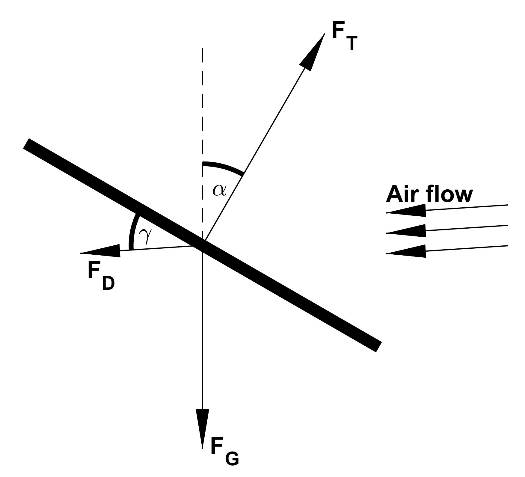
The idea behind this approach is very elegant in its simplicity. Assuming the drone is perfectly stationary, i.e., the drone has an autopilot capable of keeping the drone at the same position regardless of the wind conditions (see Appendix A.3 for a formal definition), then the tilt angle of the drone is correlated to the wind velocity. Indeed, to remain stationary under windy conditions, the autopilot has to tilt the drone such that part of the thrust force compensates for the forces generated by the wind. Figure 1 shows a force diagram of such a situation. From this figure, it becomes clear that the larger the drag (), the bigger the tilt angle ().
2.2.2. Wind Speed
There is a correlation between the drone’s tilt angle and the wind speed it experiences. According to empirical findings (see Section 3.1), this relation is best captured by a split regression of the form:
where represents the Euclidean norm, is the tilt angle and , , and are parameters to be tuned. Their values are presented in Section 3.1.
2.2.3. Wind Direction
The wind direction in the azimuthal plane is directly given by the tilt direction, i.e., the direction toward which the drone is facing when tilting.
2.3. Wind Estimation from Dynamic Model (Moving Drone)
2.3.1. General Description
This methodology aims to estimate all wind components (including vertical) and in dynamic flights. To achieve this, the method establishes a Dynamical Model (DM) of the flying drone from which wind can be inferred as a difference between model-specified and observed forces. Two specific forces influencing the drone can be identified: drag and thrust. Hence, if the total specific force and the thrust are known (observed) then the drag can be computed (Newton’s second law). Fortunately, the total specific force is known thanks to the Inertial Measurement Unit (IMU) and thrust can be estimated from the rotor speed (which is measured). Drag is the product of airflow and the resistance response of the aircraft structure plus propeller. Hence, if the latter is known thanks to an appropriate model the former can be estimated. To sum up, in order to compute air velocity one needs:
- a force model, which establishes the relation between forces in their reference frame (Section 2.3.2),
- a thrust model, which relates rotor speed to thrust (Section 2.3.4), and
- a drag model, which relates drag to air speed (Section 2.3.5 and Section 2.3.6).
The physical model proposed hereafter is inspired by the following publications about model-based navigation on small multirotor UAVs: [24,25,26]. In this work, two drag models are considered (linear and quadratic). Additionally, vertical drag is alternatively estimated or assumed to be zero (the latter removing the need for any thrust model). Hence, there are four different combinations resulting in four different estimation methods labeled as follows:
- DM, Linear and No Vertical Drag
- DM, Linear and Vertical Drag
- DM, Quadratic and No Vertical Drag
- DM, Quadratic and Vertical Drag
2.3.2. Force Model
Two specific forces are considered to act on the aircraft: thrust, which is generated by the propellers, and drag, which is generated by the flow of air around the drone. Note that lift, in the sense of deflection of air mass induced by the drone body, is not considered in this model since there are only very small lift-generating surfaces on the UAV used for testing (with the obvious exception of the propeller blades, but this is taken into account in the thrust force). Instead, the lift overcoming gravity is considered to come entirely from thrust. Hence, the expression of specific force holds:
where is the total specific force, is the specific thrust in the body frame, is the specific drag in the body frame, is the thrust in the body frame acting on the mass m, is the drag in the body frame acting on the mass m, and where the mass of the Phantom 4 RTK UAV kg. Note, that is observed directly by the IMU. Hence, using (3), the drag force can be expressed as:
Moving to the local-level frame:
In this expression, and are known through their observation and within the Inertial Navigation System (INS). Thus only the thrust force remains to be determined, which can be done as described in Section 2.3.4.
2.3.3. Force Model Assuming No Vertical Drag
With the thrust applied along the upward body axis (see Section 2.3.4) and assuming no drag in the local vertical direction, the horizontal drag components can be estimated by rewriting (5) as:
and grouping all three unknowns (, and ) in a vector , (6) can be rearranged as:
with given by:
and given by:
where indicates the inverse matrix of and designates the component on the ith line and jth column of the matrix.
2.3.4. Thrust
A simple thrust model in the body frame is commonly described by [27]:
where is the air density, b is the thrust constant of a single motor, and is the rotation rate of the i-th motor. In the case of the considered UAV, the motor thrust constant can be inferred from data produced in [28]. (The thrust constant could also be measured by observing a hovering flight with no wind, since, in this situation, thrust corresponds to weight. However, outdoor flights usually are impacted by some wind and indoor flights prevent the use of Global Navigation Satellite Systems (GNSS) which is useful for the control of hovering.) These data contain total force measurements at a given rotor speed (same for all four rotors) for a DJI Phantom 3 drone. In this case, the model can be expressed as follows:
where is the total thrust constant (since there are four identical motors) and thus
is the overall rotor speed (this relation can be found by equaling (10) and (11) and using the fact that ).
2.3.5. Quadratic Drag Model
The drag model describes a relation between the force and air speed . Along the airflow axis, the magnitude of drag can be expressed using the classic Raleigh drag equation [14]:
where is the air density, K is the drag coefficient which is dependent on the incidence angle (this assumes that the drone has a cylindrical symmetry, i.e., air flowing from the side or from the front has the same effect on the drone) (see Figure 1), and the overall rotor speed (12), and finally V is the airflow magnitude. The air speed V is the quantity of interest. All other quantities are known, except for K which is determined by leveraging that data from [28]. Selecting an experimental run in [28] with the same incidence angle and overall rotor speed, one can write:
where every quantity is known, except for K. The expression of from data in [28] is described in Section 2.3.7. V can be obtained by dividing Equation (13) by (14):
2.3.6. Linear Drag Model
Alternatively, another empirical drag model is tested where the drag force relates linearly to the air speed. In this case (13) becomes:
Thus following the same reasoning as in Section 2.3.5, air speed can be expressed as:
2.3.7. Drag from Force Data
In [28], the drag force was estimated indirectly, via the forces acting on the body that were measured. The detailed derivation of the relation between drag magnitude and measured force is presented in [29]. For a given incidence angle and overall rotor speed , the final expression is:
where is the incidence angle, is the measured force acting on the body and is the thrust force which can be estimated as described in Section 2.3.4.
2.4. Statistical Performance Metrics
2.4.1. Error, Bias, and Standard Deviation
Performance will be defined as the Euclidean distance between the reference () and the estimated quantity (). However, since wind processes are different vertically and horizontally and since two of the estimation methods consider vertical wind to be zero, the results hereafter will separate the vertical direction (local down axis) from the horizontal directions (local north and east axes). Hence horizontal wind error is defined as:
and the vertical wind error as:
Based on this error definition, bias and standard deviation are defined as usual.
2.4.2. Ground Truth
As will be discussed in Section 5.2.1, the reference sensors do not measure the wind exactly at the drone’s position. Hence, to mitigate the impact of local effects the ground truth wind is defined as the instantaneous mean of the top three sensors on the mast:
where is the wind vector as measured by the sensor placed at height h above the ground at time t.
2.4.3. Filtering in Time
The performance of filtered data will also be evaluated. The chosen filter is a low-pass finite impulse response filter with a cutoff frequency of 0.1 Hz and of order 50. This filter is applied twice on the data of interest, once in the forward direction and once in the backward direction to obtain a zero phase delay and a squared response magnitude.
2.5. Sensors
Data can be classified into two categories: flight data and reference data. Flight data contains sensor output generated by an aircraft during flight. This is the data used to make the wind estimation. Reference data contain readings of stationary wind sensors (weather stations) and is used to validate and/or calibrate drone-based wind estimations. All data is time-stamped using Coordinated Universal Time (UTC) time and acquired at a frequency of 10 Hz.
2.5.1. Flight Data
Flights were performed in Switzerland and in Norway (see Section 2.6 for flight details). In Switzerland, a DJI Phantom 4 RTK MUAV was used and, in Norway, a DJI Phantom 4 Pro MUAV was used. Both drones are the same except for the added Real-Time Kinematic (RTK) functionality of the Phantom 4. The RTK GNSS function provides the potential for positioning at centimeter-level accuracy. The RTK was set with respect to Virtual Reference Stations (VRS) provided by the Swiss Federal Office of Topography through AGNES [30]. In the rest of this work, it is assumed that both drones are the same and feature the same performance. Finally, this work uses the navigation solution (position, velocity, acceleration, and attitude) provided by the proprietary autopilot of the drone from its sensor inputs.
2.5.2. Reference Data
Reference data were produced by three different sources:
- UNISAWS: University of Svalbard (UNIS) Automatic Weather Station (AWS), situated in Adventdalen (Norway). The station measures wind at 2 and 10 m above ground together with several other atmospheric parameters. Its sensor characteristics can be found in Table 2.
- MoTUS: Urban microclimate measurement mast, situated on the campus of the École Polytechique Fédéral de Lausanne (EPFL) (Switzerland). The mast features seven sonic anemometers, spread vertically up to a height of approx. 22 m above ground. Table 3 details its sensor characteristics.
- TOPOAWS: TOPO Automatic Weather Station. This is a small portable weather station developed by the Geodetic Engineering Lab (TOPO) at EPFL. Wind is measured using a cup anemometer and an 8-direction wind vane. Table 4 describes the sensor characteristics.
2.6. Flight Campaign
During this work, two flight campaigns were performed: one in Norway and one in Switzerland. A total of 75 flights were conducted, where a flight is defined as the time interval between take-off and landing. The drone used is a DJI Phantom 4 (see Section 2.5.1 for details).
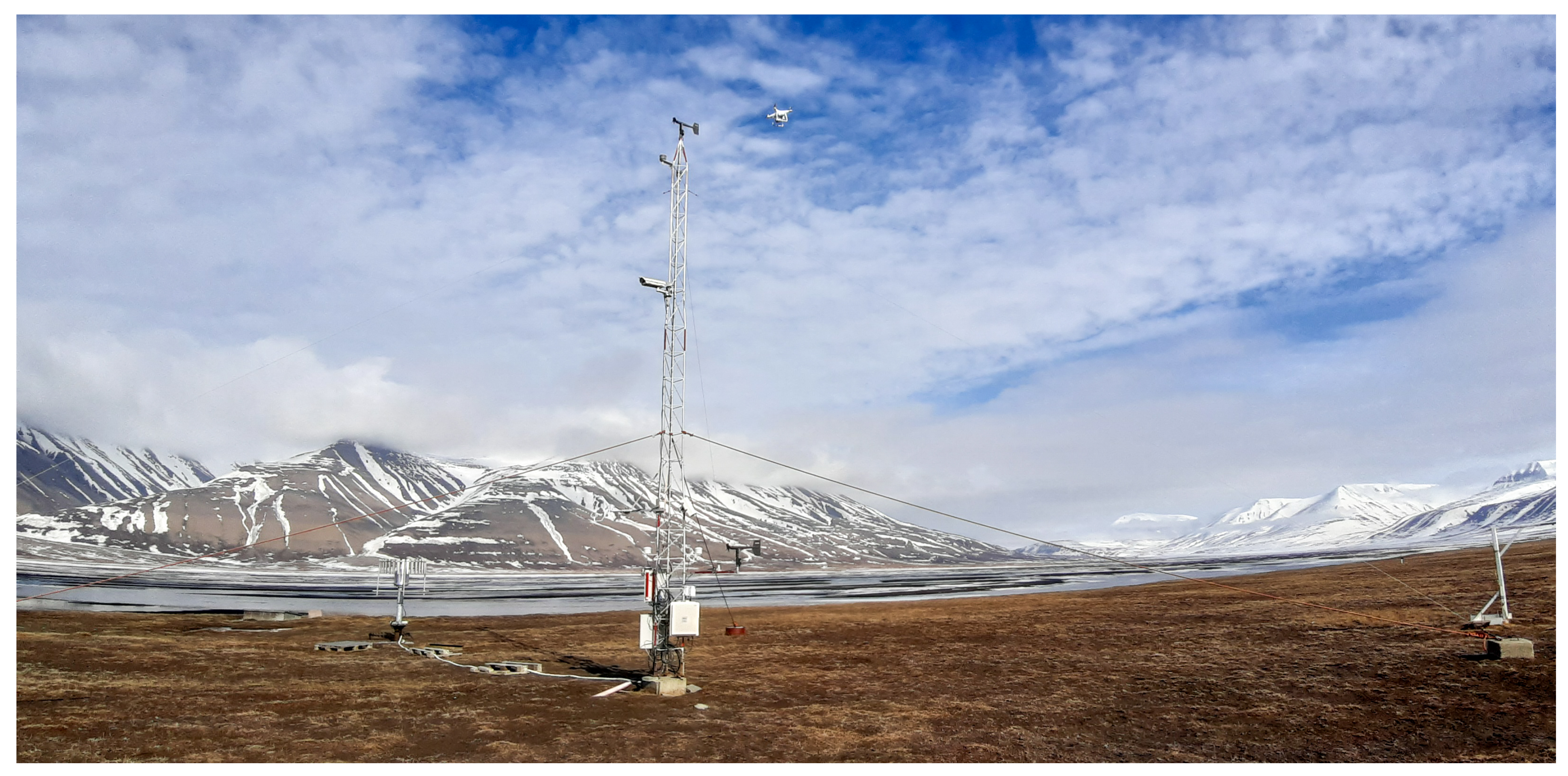
In Norway, 19 flights spread over 12 different days were executed. Flights were performed in Adventdalen next to the UNISAWS which is the source of the reference measurements used for these flights. This flight campaign only features stationary flights at an altitude of 2 m and 10 m above ground and at a distance of 10 m from the weather station. Figure 2 shows the position of the weather station with respect to Longyearbyen.
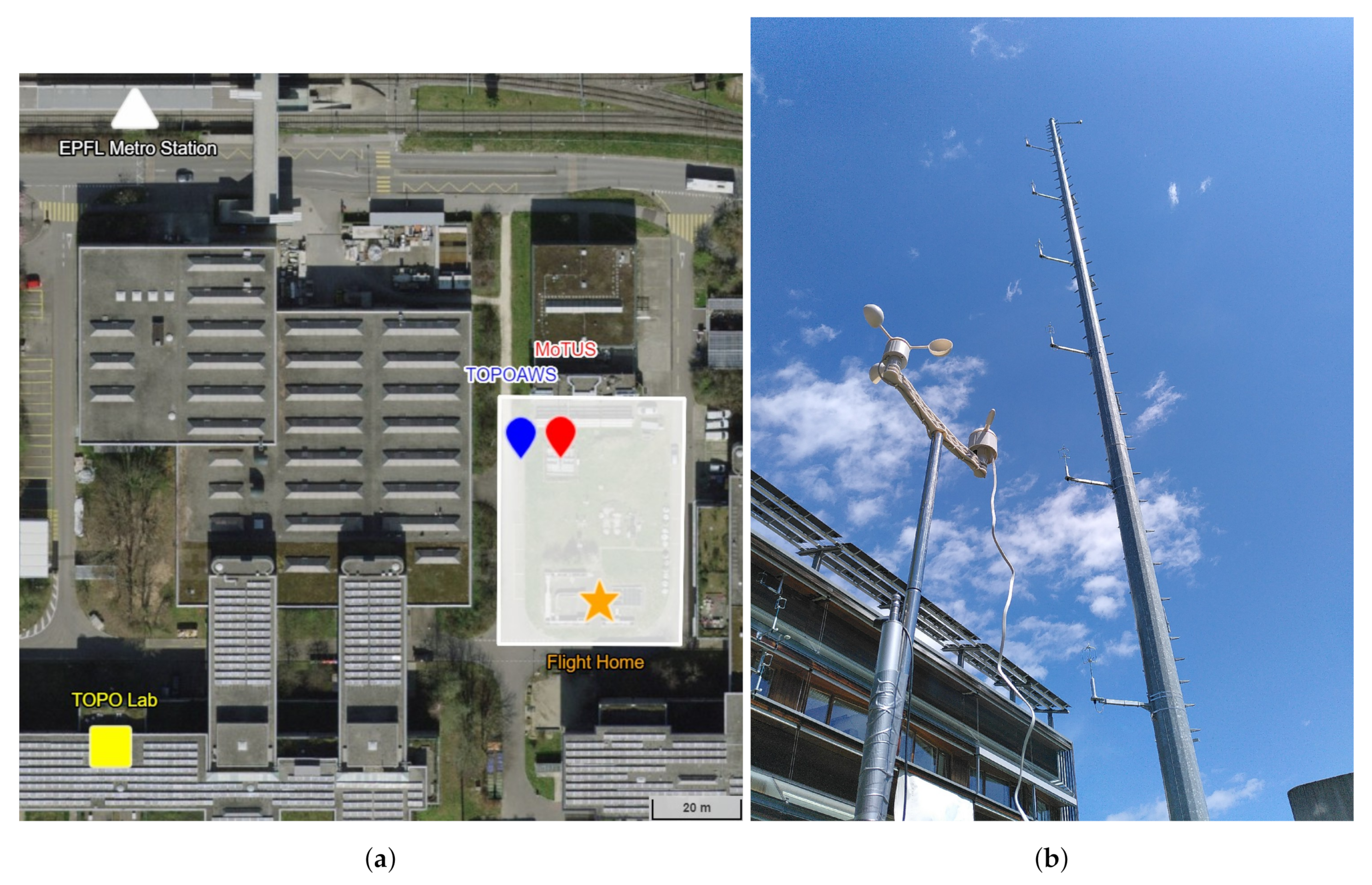
In Switzerland, 56 flights spread over 6 different days were executed. Flights were performed on EPFL’s campus in the flight zone shown in Figure 3. This location was chosen because of the presence of the MoTUS weather mast from which wind reference measurements were obtained. All flights were performed above roof height, i.e., approximately 15 m above ground or higher, to mitigate the effect of turbulence generated by buildings.
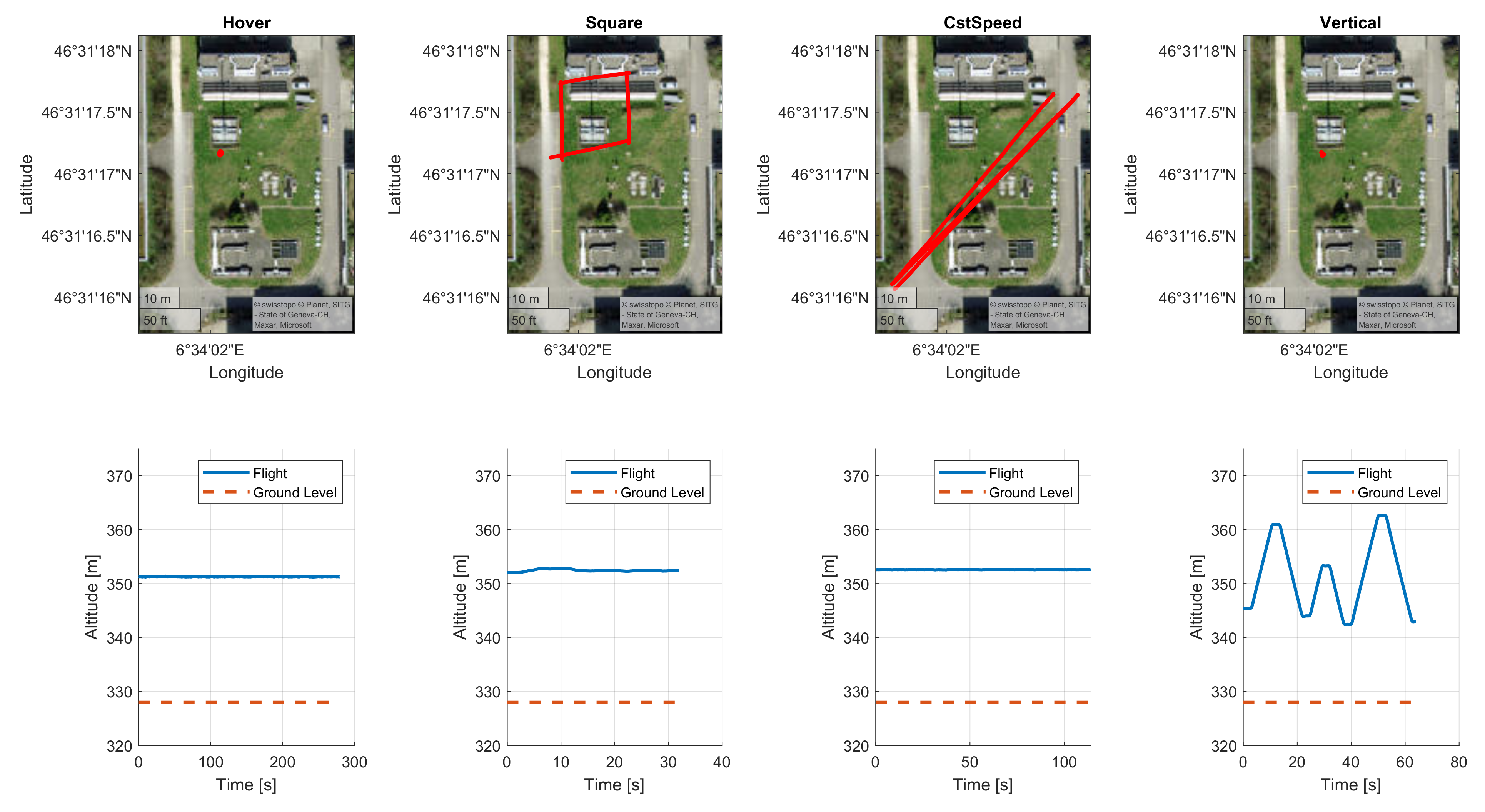
The flights were performed using the Phantom’s autopilot in waypoint mode, which allows a set of waypoints to be defined over which the drone will fly as well as a maximal cruising speed. A waypoint is defined by its latitude, longitude, altitude, and heading. A set of waypoints and their cruising speed is stored as a flight plan in the drone’s remote control and will be called a flight type in this work. Ten different flight types were defined that can be grouped into four categories (see Figure 4):
- Hover: Using two waypoints (a flight plan with only one waypoint is not valid on the DJI Phantom 4 RTK), the drone moves to an altitude of approximately 20 m above ground and 10 m to the south of the weather mast. Once the final waypoint is reached the drone hovers (holds its position), its body x-axis pointing roughly toward the north. The pilot decides when the position hold ends, typically after 5 to 10 min.
- Square: The drone moves in an approximate square with a side length of 20 m. The square is centered on the weather mast. The drone’s attitude is such that the body x-axis is pointed toward the weather mast during the whole flight (i.e., the drone’s camera is always looking at the mast).
- Constant speed (cstSpeedXms): The drone moves approximately from the northeast corner of the flight zone to its southwest corner then back and then to the southwest corner again (three segments in total). The heading is always in the travel direction. This flight plan is repeated four times at cruising speeds of 2, 6, 10, and 13 m/s, respectively (Thus the flights are named cstSpeed2ms, cstSpeed6ms, cstSpeed10ms, and cstSpeed13ms respectively).
- Vertical (VerticalXms): The drone moves to the same horizontal position as during the hover flight, but at an altitude of 15 m above ground. Then it moves up and down three times to approximately 30 m above ground and back to 15 m. During the maneuver, the body x-axis is always pointing north. This flight plan is repeated four times at cruising speeds of 2, 3, 4 and 5 m/s, respectively (thus the flights are named Vertical2ms, Vertical3ms, Vertical4ms, and Vertical5ms respectively).
Figure 4.
Flight types. Plots on the upper row show a typical flight as seen from above (see Figure 3). Plots on the lower row show the drone’s altitude over time. From left to right, plotted flights are hover, square, cstSpeed2ms, and Vertical2ms.
Figure 4.
Flight types. Plots on the upper row show a typical flight as seen from above (see Figure 3). Plots on the lower row show the drone’s altitude over time. From left to right, plotted flights are hover, square, cstSpeed2ms, and Vertical2ms.

3. Model Parameters
3.1. Tilt Model
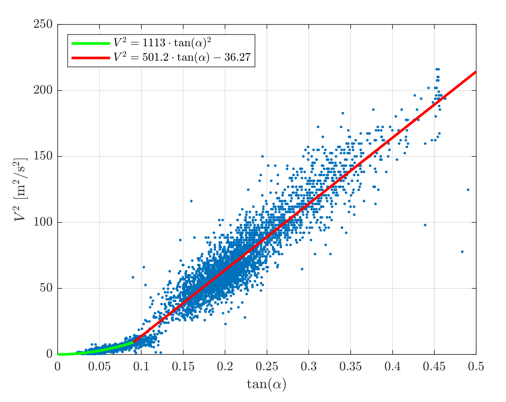
Figure 5 shows the calibration dataset for a DJI Phantom 4 Pro. This dataset is composed of flights performed in Norway next to the UNISAWS sensors (see Section 2.6). The figure indicates the correlation between the tangent of the tilt angle, , and the air velocity squared . The tuned parameters to be used in Equation (2) for the Phantom 4 are listed in Table 5.
3.2. Thrust Model
3.3. Drag Model
4. Results
This section will evaluate the wind estimation of three arbitrarily chosen flights from the EPFL campaign:
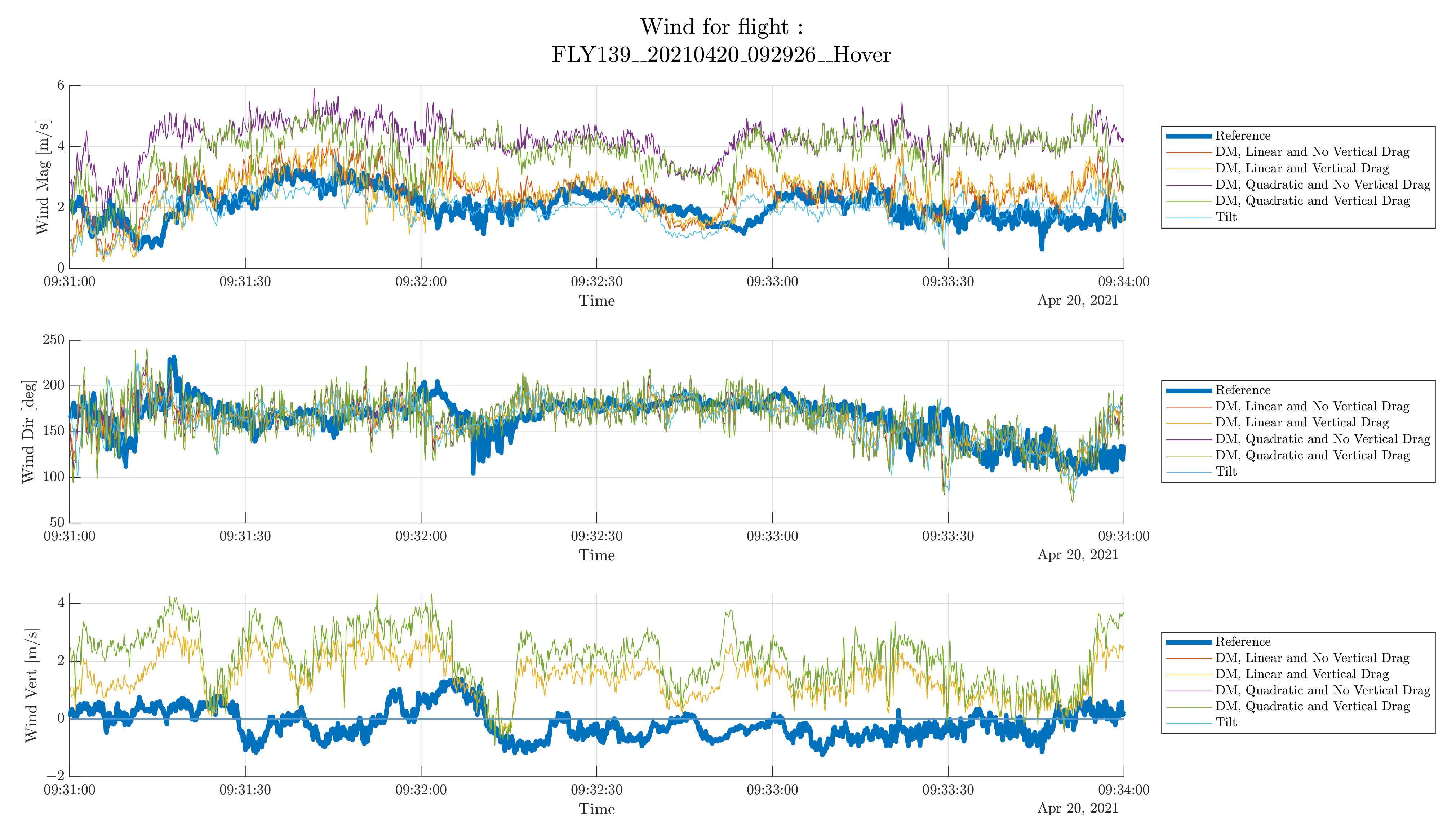
Note that no flight of type cstSpeed is detailed here, as this scenario shows very similar performance to square flights at high flight speeds and to hover flights at low speed. Figure 7 shows the wind vector decomposed as horizontal wind speed (top plot), horizontal wind direction (center plot), and vertical wind (bottom plot). On each plot, the thick blue curve represents the ground-truth data acquired from the external anemometer and the other curves represent the data resulting from each estimation method. Table 6 shows the statistical performance of each method as defined in Section 2.4. It is worth noting that for the horizontal wind, the norm of the bias is shown (not the bias vector). The three selected flights will be evaluated individually below.
4.1. Hover
The hover flight type is important to consider as it is the only flight type where the assumptions underlying the Tilt estimation method (see Section 2.2) are respected. In other words, it is the only flight type where the tilt estimation method has a “fair” comparison. On the other hand, any estimation method should perform at least as well as the tilt method in this simple case. Note that the data plotted in Figure 7 show only three min of the total flight in order to allow for detailed features of the measurements visible.
4.1.1. Horizontal Wind Speed
Starting with the horizontal wind magnitude and looking at the tilt estimation (light blue curve), it can be seen that it produces a good approximation of the actual horizontal wind. Variations in the wind speed seem to be reflected in the estimation. An exception to this could be the small wind gust present around 09:33 (blue highlight in Figure 7). In the reference data, this gust crosses the 2 m/s mark at 09:32:59, and in the tilt estimation at 09:32:54, this is a difference of 5 s. Knowing that the drone flies approximately 10 m to the south of the wind reference and that the wind is coming from the south, it seems reasonable to assume that the cause of this delay is due to the propagation time of this wind gust and not a data synchronization issue. Considering the proposed estimation methods, they can be grouped in pairs: the two methods using the linear drag model perform very similarly and are also a good estimation of the true wind speed (bias of 0.29 m/s and standard deviation of 0.82 m/s for the filtered DM with vertical drag); the two methods using the quadratic drag model perform also very similar but seem to feature an important bias (1.9 m/s for the DM with no vertical drag). This highlights two important observations. First, assuming that the vertical wind speed is zero has minimal impact on the estimation of horizontal wind speed. This will be further discussed in Section 5.1.1. Second, the choice of drag model has a significant impact on the estimation. This will be further discussed in Section 5.1.2. Additionally, the filtered estimations show an improved performance of approximately 20 % on the standard deviation, as could be expected from filtering.
4.1.2. Horizontal Wind Direction
Observing the wind direction on the middle plot, it can be seen that all five estimation methods perform very similarly and give a fairly good estimation of the wind direction. The only slight difference concerns the two methods using the quadratic drag model, which have higher variability. There seems to be a “directional wind gust” around 09:32 (red highlight in Figure 7), which results in what appears to be a timing mismatch between estimation and measurement. However, as for wind speed, it seems fair to assume that this is due to wind gust propagation time between the respective position of the drone and its reference.
4.1.3. Vertical Wind
Finally, looking at the vertical wind speed, it can first be seen that even if the vertical wind speed is not zero, in the evaluated use case it remains close to 0 m/s. Thus, assuming that there is no vertical wind speed is a reasonable assumption. In this case, the methods estimating vertical wind have worse performance than the errors caused by the assumption of the vertical wind being null.
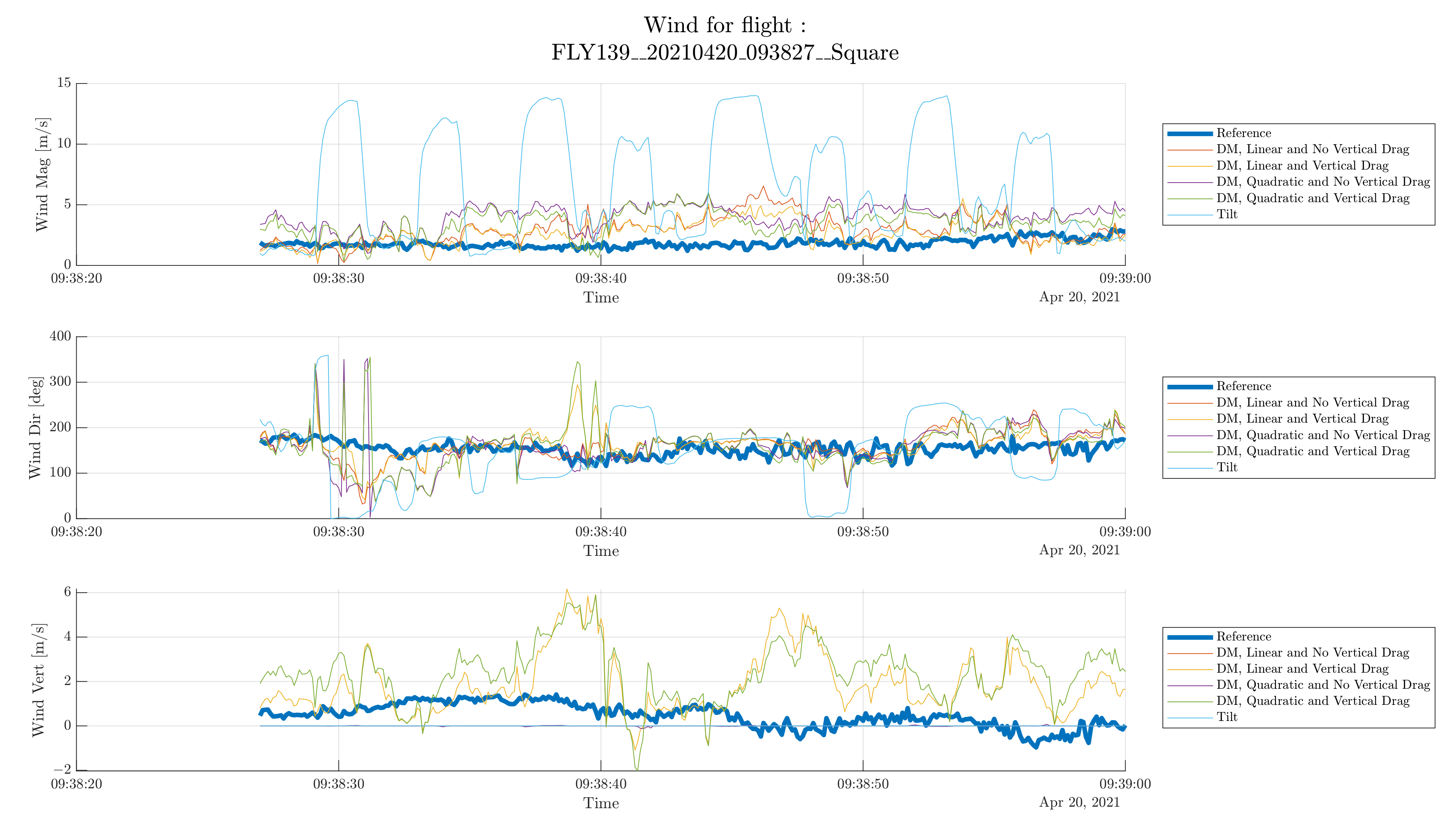
4.2. Square
The square flight is interesting due to its dynamics: accelerations are high when reaching or leaving the corner of the square thus inducing tilting of the UAV due to forward motion. The first obvious observation to be made about the estimations seen in Figure 8, is that the tilt estimation is failing at estimating wind speed and direction in such a flight scenario, which is expected. The error peaks (as for example in the blue highlight in Figure 8) can be traced back to the moments of drone acceleration or deceleration. On the other hand, the dynamic model-based methods, seem to be able to filter out the impact of the vehicle acceleration. Although this comes at the cost of some loss in accuracy, as can be seen by comparing Table 6 and Table 7. Wind direction seems to be estimated correctly most of the time by the dynamic model-based methods, except for some occurrences where its estimation is completely wrong, such as around 09:38:30 (red highlight) or 09:38:40 (yellow highlight). It is unclear why this is happening. However, the low wind speed estimated (less than 1 m/s) during both time intervals may have reduced the reliability of this polar parameterization. Concerning vertical wind, the same observations can be made as those in the hover flight.
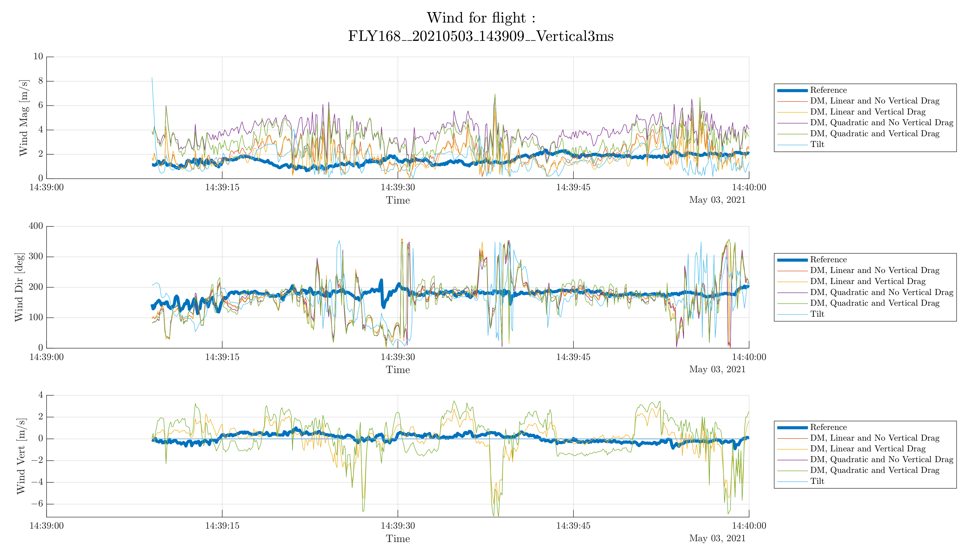
4.3. Vertical
The vertical flight is interesting for its application in shear wind estimation. The most important observation to make in Figure 9 is that there are three phases where the estimation significantly deviates from the reference. These phases are highlighted in red and correspond to the moments where the drone is descending. Moving downward is notoriously difficult for a drone since it flies inside the downwash produced by its propellers. For this reason, the downward flight is very unstable, resulting in large and fast attitude variation, in turn leading to poor wind estimations. However, estimation during the ascending phase (highlighted in blue) seems to produce accurate results, in particular for tilt and linear drag dynamic model estimation methods.
5. Discussion
5.1. Outcomes
5.1.1. Impact of Vertical Wind Estimation
As presented in Section 1, vertical wind is rarely considered in the literature, either to reduce estimation complexity or to remove the need for rotor thrust estimations. It also removes the need to have a reference capable of measuring vertical wind, such as a through use of a sonic anemometer. Two important observations can be made based on the results presented in Section 4. First, horizontal wind estimation performance for the methods assuming no vertical wind is not different from those which estimate vertical wind. This is likely due to the fact that the vertical wind was close to zero during all flights which were conducted at low altitudes. Thus estimating thrust using the wind tunnel data leads to similar results as computing it from Equation (7). However, before choosing methods including vertical drag over methods assuming no vertical drag, it would be relevant to compare the performance of both approaches on data featuring significant vertical wind. Second, for methods estimating vertical wind, the estimation is rather poor. The error is smaller by assuming the value of vertical wind to be zero. This is somewhat surprising as air speed is computed in the body frame, and thus one should assume that the estimation accuracy of vertical and horizontal wind should be similar. The observed discrepancy may be due to the fact that the thrust is much larger than the drag in the vertical direction but not in the horizontal direction. Hence, even a small error in thrust estimation leads to a large error in vertical wind estimation.
5.1.2. Linear or Quadratic Drag Model
Two drag models were explored during this work: a quadratic model, presented in Section 2.3.5 and a linear model, presented in Section 2.3.6. The quadratic model is well tested for spherical objects and widely used to model drag forces on MUAVs [39]. However, in this work, for low wind speeds (less than 10 m/s), the linear drag model performs better in the estimation of wind speed. This is somewhat surprising given that all publications presented in Section 1 which employ a physical model for drag, use a quadratic drag model. However, this observation is not new in MUAV modeling: for example [39] analytically derives and experimentally validates a linear drag relation using Blade Element Momentum (BEM) theory. Plus, the well-known open-source Gazebo simulator also implements a linear drag model for MUAVs [40]. According to this model the total drag force is dominated by drag generated by air passing through the rotors in the xy-body-plane, i.e., perpendicularly to the thrust direction. More explicitly, the drag model for a single rotor is given by:
This is not the linear model implemented in this work, but both models are equivalent under the assumptions that the rotor angular rates are constant and the drone is not tilting. Note also that BEM-based approaches start to fail at high air speeds and other approaches are needed to correct drag modeling, see for example [41], where BEM is combined with a neural network trained to estimate drag residuals that BEM theory is not able to predict.
5.2. Dataset Limitations
5.2.1. Distance to Reference Sensors
Reference measurements in UAV based wind measurements are always a challenge since there is a geometrical separation between the UAV’s position and the reference sensor. Additionally, the further the reference sensor is placed from the drone, the higher the chances that local wind gusts affect either only the drone or the reference sensor or affect both at different times. In an extreme case, when the flow is purely turbulent, it is not meaningful to compare wind speed from two sensors if they are not at the same position (if the experiment takes place in a wind tunnel providing good laminar flow, these problems can be avoided at the cost of a less realistic wind behavior). In this dataset, the drone was flying approximately 10 to 15 m away from the reference sensor. This separation ensured the safety of hardware and infrastructure but constitutes a significant distance to the reference sensors. For example, at a wind speed of 2 m/s, this can represent a propagation delay of 5 s.
5.2.2. Environmental Variability
The validation dataset was acquired over one flight zone (Figure 3), which has its typical environmental conditions. It would be interesting to introduce more variability of environmental conditions to explore their effects. Interesting environments to explore could be for example open field (without buildings), high altitude above sea level and above ground, low temperature (close to freezing), high latitude, terrain with high convection current, etc. Obviously, the main challenge in such experiments is to obtain a reliable reference measurement that allows the evaluation of the estimation performance. Additionally, acquisitions in stronger winds would also improve the dataset.
5.2.3. Ground Truth Quality
The quality of ground truth was assessed by computing the difference between each of the three reference sensors and their mean. In other words, the error (as defined in (19) and (20)) for all the reference sensors. Let this error be the ground truth error. The reference sensor data is shown in Figure 10 and the ground truth error statistics are shown in Table 9. The ground truth error is expected to be small if there is no turbulence and no local effects, which is a necessary assumption to compare the drone’s wind estimation to the reference. However, the ground truth error can get large. In this sample flight, the difference between the mean and a given sensor can be on the order of 1 m/s (yellow highlight in Figure 10). Note also that the wind gusts identified in Figure 7 also correspond to moments of high ground truth error (blue and red highlight in both figures). This leads to the conclusion that the impact of turbulence might have been underestimated in the test environment and that many cases are approaching the accuracy of the reference.
The quality of the reference represents a hard limit to the development of new estimation methods because it prevents the evaluation of their performance beyond the reference accuracy. It is essential to find some alternative reference, that provides measurements that are closer to the aircraft body. This remains an open question, but two possible approaches can be explored here. First, consider only time-averaged data over longer periods (averaging time greater than one min): this approach is easy to implement and should remove most of the high-frequency variability, at the cost of reducing the estimation’s bandwidth. Second, perform indoor flights where there is no wind: in this scenario, the air speed is equal to the vehicle speed, thus the method can be validated by verifying how well it estimates vehicle speed for which a ground truth can be provided by a motion capture system. This approach is similar to what is done in [41]. However, this solution assumes that the effect of traveling at a given speed in still air is the same as hovering in a wind of the same speed. Plus, the used drone must be able to navigate without access to GNSS positioning, since the reception of satellite signals is not available indoors.
5.3. Method Trade-Off
This section lists pros (+) and cons (−) of the tested estimation methods. The estimation methods using the quadratic drag model are not included since, within the conducted experiments, they are out-performed by the other methods. Still, these may be worth considering at higher wind speeds than those encountered in this work.
- DM, Linear without Vertical Drag
- +
- Most precise and accurate during dynamic maneuvers, thus enabling continuous profiling.
- +
- Does not need to estimate thrust.
- +
- Relies only on pose estimation not on the drone’s control loop.
- −
- Does not estimate vertical wind, which may impact estimation accuracy.
- −
- Less precise than tilt method in hovering conditions.
- −
- Needs wind tunnel data (for each UAV type) to compute drag coefficients.
- DM, Linear with Vertical Drag
- +
- Most precise and accurate during dynamic maneuvers, thus enabling continuous profiling.
- +
- Relies only on pose estimation not on the drone’s control loop.
- (+)
- Attempts to estimate vertical wind, but results are poor.
- −
- Less precise than tilt in hovering conditions.
- −
- Needs wind tunnel data (for each UAV type) to compute drag coefficients.
- Tilt
- +
- Most accurate and precise during hovering.
- +
- Simple to describe and implement.
- +
- Simple to extrapolate to other platforms, provided calibration flights are possible.
- −
- Limited to hovering and slowly ascending flights.
- −
- Does not estimate vertical wind, which may impact estimation accuracy.
- −
- Depends on the performance of autopilot control.
5.4. Comparison with On-Board Flow Sensor Approach
Here we relate the performance of the proposed methods to that presented in [8] that employs dedicated wind sensor (four-hole pressure probe, pitot tube) mounted far away from the rotor-blades on a MULTIROTOR G4 Eagle drone. The comparison with this work is especially relevant since the experiments took place at the same location on the campus (see Figure 3) and using the same sonic anemometers as a reference. Table 10 compares the statistical evaluation of the hover wind estimation within the flight presented in Section 4.1 with the performance obtained in [8] (only DM, Linear wind, No Vertical Drag is shown for clarity). Test 4, presented in Table 2 of [8], was chosen for comparison since it featured the most similar wind conditions.
It is interesting to see that both approaches feature a similar bias, but the precise onboard flow sensor has a considerably lower standard deviation. Overall, the performance of the two approaches is very similar. However, the approach presented in this work does not require the additional integration of a custom-made special sensor on the UAV. This impacts the cost, size, and reliability of the instrumentation. Additionally, the necessity of the long arm on which the wind sensor needs to be mounted is likely to make the drone less stable. Additionally, the use of a single pressure probe makes the navigation more complex since the sensor must always point upstream. For all of the above-listed reasons, the authors believe that the presented inertial-based approach represents an interesting alternative that can be further developed.
6. Conclusions
6.1. Summary
The main contributions of this work are:
- Validating the tilt method with empirical data using an off-the-shelf drone, making it easily implementable by others.
- Proposing a novel and more general estimation scheme, usable on a commercial drone, which performs similarly to the tilt approach in hovering conditions while at the same time capable of producing wind estimations during dynamic flights.
- Empirically assessing the impact of ignoring the vertical wind component on horizontal wind estimation.
6.2. Perspectives
Future work should focus on three main aspects. First, further validate the quality of the proposed estimation methods. This can be achieved by addressing the ground truth quality issue discussed in Section 2.4.2. Additionally, increasing the test dataset size with new flights performed in different environmental conditions (e.g., in stronger wind, in presence of convection, at higher altitude, at lower temperatures, etc.) to confirm the method’s generality.
The second aspect which deserves further attention is the improvement of the drag model. As discussed in Section 5.1.2, different theories may be more suitable to model the drag of small MUAV. Additionally, acquiring a dataset of varying wind in a wind tunnel may also help to identify a suitable drag model. A Computational Fluid Dynamics (CFD) simulation could also be performed to attempt to better understand the impact of drag on the UAV.
Following up on [24,42], the results of this work will be of use in the improvement of the model-based navigation developed by one of the co-authors. This development was so far based on simulations, but this study provides empirical data on which the navigation solution can be tested. Additionally, a dedicated (non-commercial) UAV platform was developed that is expected to overcome some limitations of the current hardware. Namely, this UAV features direct thrust sensors and an inertial sensor of better quality. An evaluation of the performance improvements due to improved sensor quality is planned in the near future.
Finally, future work may aim at developing an application with a user-friendly interface, such that this estimation method can be easily shared within the research community.
The authors recommend continuing the development of this estimation scheme as it has demonstrated promising results and has the potential to be applied in various fields. As already discussed in Section 1, such applications include boundary layer measurements, wind turbine wake measurements, weather observations, to name a few. The approach also can also serve as an alternative to disposable weather balloons.
Author Contributions
Conceptualization, K.M., R.H., J.S. and A.G.; methodology, K.M., R.H., J.S. and A.G.; software, K.M. and A.G.; validation, R.H. and J.S.; formal analysis, K.M. and A.G.; investigation, K.M., R.H. and A.G.; resources, R.H. and J.S.; data curation, K.M. and A.G.; writing—original draft preparation, K.M.; writing—review and editing, K.M., R.H., J.S. and A.G.; visualization, K.M.; supervision, R.H. and J.S.; project administration, R.H. and J.S.; funding acquisition, R.H. and J.S. All authors have read and agreed to the published version of the manuscript.
Funding
The work is partially supported by the Schweizerischer Nationalfonds zur Förderung der Wissenschaftlichen Forschung (Swiss National Science Foundation, SNSF). Reference: 200021_182072. Fieldwork in Norway was funded by the Norges Forskningsråd (Research Council of Norway, RCN) through the Arctic Field Grant, provided by the Svalbard Science Forum (SSF). Reference: RiS ID, 11372. The work is also partly sponsored by the RCN through the Centre of Excellence funding scheme. Reference: 223254 (AMOS).
Data Availability Statement
All flight and weather data is available [43]. Source code is available on GitHub at https://github.com/meierkilian/WEMUAV (accessed on 17 February 2022).
Acknowledgments
The authors thank Marius Jonassen at the University Centre in Svalbard for his active support of the project.
Conflicts of Interest
The authors declare no conflict of interest.
Abbreviations
The following abbreviations are used in this manuscript:
| ABL | Atmospheric Boundary Layer |
| BEM | Blade Element Momentum |
| CFD | Computational Fluid Dynamics |
| DM | Dynamic Model |
| FRD | Front-Right-Down |
| GNSS | Global Navigation Satellite System |
| IMU | Inertial Measurement Unit |
| INS | Inertial Navigation System |
| MoTUS | Urban Microclimate Measurement Mast |
| MUAV | Multirotor UAV |
| NED | North-East-Down |
| RPAS | Remotely Piloted Aircraft Systems |
| RTK | Real-Time Kinematic |
| TOPOAWS | TOPO Automatic Weather Station |
| UAS | Unmanned Aircraft Systems |
| UAV | Unmanned Aerial Vehicles |
| VRS | Virtual Reference Station |
Appendix A. Notations
This appendix will briefly introduce the notation conventions used throughout this work. Detailed notation and definitions of reference frames can be found in [44,45].
Appendix A.1. Vectors
Vectors are noted using a single lowercase letter in bold. The letter may feature a superscript indicating the frame the vector is expressed in ().
Appendix A.2. Rotation Matrices and Quaternions
Rotation matrices are denoted using the uppercase character in bold. Quaternions are noted using a lowercase character written in bold. The respective superscript and subscript indicate the two frames the rotation is relating to. For example, a rotation matrix defining the rotation from frame i to j is written as and a quaternion as .
Appendix A.3. Reference Frames and Hovering
Three main frames are used in this work:
- Inertial frame (i-frame): a non-accelerating and non-rotating frame in which Newtonian mechanics holds (up to the observation precision).
- Local-level (l-frame): local-leveled geodetic frame such that its axes point respectively North, East, and Down (NED), with respect to the reference surface (e.g., ellipsoid).
- Body frame (b-frame): frame fixed to the drone such that its axes point Forward, to the Right and Downward (FRD).
Hovering is thus defined as a constant position in the local-level frame (), i.e., stationary with respect to the ground. The expressions “hovering” and “stationary flight” are used interchangeably.
References
- O’Shea, O.R.; Hamann, M.; Smith, W.; Taylor, H. Predictable pollution: An assessment of weather balloons and associated impacts on the marine environment—An example for the Great Barrier Reef, Australia. Mar. Pollut. Bull. 2014, 79, 61–68. [Google Scholar] [CrossRef] [PubMed]
- Anderson, K.; Gaston, K.J. Lightweight unmanned aerial vehicles will revolutionize spatial ecology. Front. Ecol. Environ. 2013, 11, 138–146. [Google Scholar] [CrossRef] [Green Version]
- Reuder, J.; Brisset, P.; Jonassen, M.M.; Mayer, S. The Small Unmanned Meteorological Observer SUMO: A new tool for atmospheric boundary layer research. Meteorol. Z. 2009, 18, 141–147. [Google Scholar] [CrossRef]
- Hann, R.; Altstädter, B.; Betlem, P.; Deja, K.; Dragańska-Deja, K.; Ewertowski, M.; Hartvich, F.; Jonassen, M.; Lampert, A.; Laska, M.; et al. Scientific Applications of Unmanned Vehicles in Svalbard; SESS Report 2020; Svalbard Integrated Arctic Earth Observing System: Longyearbyen, Norway, 2020. [Google Scholar] [CrossRef]
- Lampert, A.; Altstädter, B.; Bärfuss, K.; Bretschneider, L.; Sandgaard, J.; Michaelis, J.; Lobitz, L.; Asmussen, M.; Damm, E.; Käthner, R.; et al. Unmanned Aerial Systems for Investigating the Polar Atmospheric Boundary Layer—Technical Challenges and Examples of Applications. Atmosphere 2020, 11, 416. [Google Scholar] [CrossRef] [Green Version]
- Subramanian, B.; Chokani, N.; Abhari, R.S. Drone-Based Experimental Investigation of Three-Dimensional Flow Structure of a Multi-Megawatt Wind Turbine in Complex Terrain. J. Sol. Energy Eng. 2015, 137, 051007. [Google Scholar] [CrossRef]
- Subramanian, B.; Chokani, N.; Abhari, R. Experimental analysis of wakes in a utility scale wind farm. J. Wind. Eng. Ind. Aerodyn. 2015, 138, 61–68. [Google Scholar] [CrossRef]
- Fuertes, F.C.; Wilhelm, L.; Porté-Agel, F. Multirotor UAV-Based Platform for the Measurement of Atmospheric Turbulence: Validation and Signature Detection of Tip Vortices of Wind Turbine Blades. J. Atmos. Ocean. Technol. 2019, 36, 941–955. [Google Scholar] [CrossRef]
- Prudden, S.; Fisher, A.; Marino, M.; Mohamed, A.; Watkins, S.; Wild, G. Measuring wind with Small Unmanned Aircraft Systems. J. Wind. Eng. Ind. Aerodyn. 2018, 176, 197–210. [Google Scholar] [CrossRef]
- Mayer, S.; Hattenberger, G.; Brisset, P.; Jonassen, M.O.; Reuder, J. A ‘No-Flow-Sensor’ Wind Estimation Algorithm for Unmanned Aerial Systems. Int. J. Micro Air Veh. 2012, 4, 15–29. [Google Scholar] [CrossRef] [Green Version]
- Khaghani, M.; Skaloud, J. Assessment of VDM-based autonomous navigation of a UAV under operational conditions. Robot. Auton. Syst. 2018, 106, 152–164. [Google Scholar] [CrossRef]
- Khaghani, M.; Skaloud, J. Evaluation of Wind Effects on UAV Autonomous Navigation Based on Vehicle Dynamic Model. In Proceedings of the 29th International Technical Meeting of The Satellite Division of the Institute of Navigation (ION GNSS+ 2016), Portland, OR, USA, 12–16 September 2016; pp. 1432–1440. [Google Scholar] [CrossRef]
- Neumann, P.P.; Bartholmai, M. Real-time wind estimation on a micro unmanned aerial vehicle using its inertial measurement unit. Sens. Actuators A Phys. 2015, 235, 300–310. [Google Scholar] [CrossRef]
- Palomaki, R.T.; Rose, N.T.; van den Bossche, M.; Sherman, T.J.; De Wekker, S.F.J. Wind Estimation in the Lower Atmosphere Using Multirotor Aircraft. J. Atmos. Ocean. Technol. 2017, 34, 1183–1191. [Google Scholar] [CrossRef]
- Song, Y.; Luo, B.; Meng, Q.H. A rotor-aerodynamics-based wind estimation method using a quadrotor. Meas. Sci. Technol. 2018, 29, 025801. [Google Scholar] [CrossRef] [Green Version]
- Xing, Z.; Zhang, Y.; Su, C.Y.; Qu, Y.; Yu, Z. Kalman Filter-based Wind Estimation for Forest Fire Monitoring with a Quadrotor UAV. In Proceedings of the 2019 IEEE Conference on Control Technology and Applications (CCTA), Hong Kong, China, 19–21 August 2019; pp. 783–788. [Google Scholar] [CrossRef]
- Wang, L.; Misra, G.; Bai, X. A K Nearest Neighborhood-Based Wind Estimation for Rotary-Wing VTOL UAVs. Drones 2019, 3, 31. [Google Scholar] [CrossRef] [Green Version]
- Perozzi, G.; Efimov, D.; Biannic, J.M.; Planckaert, L. Using a quadrotor as wind sensor: Time-varying parameter estimation algorithms. Int. J. Control. 2020, 95, 126–137. [Google Scholar] [CrossRef]
- Qu, Y.; Wang, K.; Wu, X. Wind Estimation with UAVs Using Improved Adaptive Kalman Filter. In Proceedings of the 2019 Chinese Control And Decision Conference (CCDC), Nanchang, China, 3–5 June 2019; pp. 3660–3665. [Google Scholar]
- Abichandani, P.; Lobo, D.; Ford, G.; Bucci, D.; Kam, M. Wind Measurement and Simulation Techniques in Multi-Rotor Small Unmanned Aerial Vehicles. IEEE Access 2020, 8, 54910–54927. [Google Scholar] [CrossRef]
- González-Rocha, J.; De Wekker, S.F.J.; Ross, S.D.; Woolsey, C.A. Wind Profiling in the Lower Atmosphere from Wind-Induced Perturbations to Multirotor UAS. Sensors 2020, 20, 1341. [Google Scholar] [CrossRef] [Green Version]
- Allison, S.; Bai, H.; Jayaraman, B. Wind estimation using quadcopter motion: A machine learning approach. Aerosp. Sci. Technol. 2020, 98, 105699. [Google Scholar] [CrossRef] [Green Version]
- Loubimov, G.; Kinzel, M.P.; Bhattacharya, S. Measuring Atmospheric Boundary Layer Profiles Using UAV Control Data; AIAA Scitech 2020 Forum; American Institute of Aeronautics and Astronautics: Orlando, FL, USA, 2020. [Google Scholar] [CrossRef]
- Crocoll, P.; Seibold, J.; Scholz, G.; Trommer, G.F. Model-Aided Navigation for a Quadrotor Helicopter: A Novel Navigation System and First Experimental Results: Model-Aided navigation for a quadrotor helicopter. Navigation 2014, 61, 253–271. [Google Scholar] [CrossRef]
- Crocoll, P.; Trommer, G.F. Quadrotor inertial navigation aided by a vehicle dynamics model with in-flight parameter estimation. In Proceedings of the 27th International Technical Meeting of the Satellite Division of The Institute of Navigation (ION GNSS+ 2014), Tampa, FL, USA, 8–12 September 2014; pp. 1784–1795. [Google Scholar]
- Heidari, H.; Saska, M. Collision-free trajectory planning of multi-rotor UAVs in a wind condition based on modified potential field. Mech. Mach. Theory 2021, 156, 104140. [Google Scholar] [CrossRef]
- Bouabdallah, S. Design and Control of Quadrotors with Application to Autonomous Flying. Ph.D. Thesis, EPFL, Lausanne, Switzerland, 2007. [Google Scholar]
- Russell, C.; Jung, J.; Willink, G.; Glasner, B. Wind Tunnel and Hover Performance Test Results for Multicopter UAS Vehicles; Technical Memorandum NASA/TM–2018–219758; NASA Ames Research Center: Mountain View, CA, USA, 2018.
- Schiano, F.; Alonso-Mora, J.; Rudin, K.; Beardsley, P.; Siegwart, R.; Sicilianok, B. Towards estimation and correction of wind effects on a quadrotor UAV. In Proceedings of the IMAV 2014: International Micro Air Vehicle Conference and Competition, Delft, The Netherlands, 12–15 August 2014; pp. 134–141. [Google Scholar]
- Brockmann, E.; Wild, U.; Ineichen, D.; Grünig, S. Automated GPS Network in Switzerland (AGNES); Activity Report; International Foundation HFSJG: Bern, Switzerland, 2004. [Google Scholar]
- Datasheet Young 05103. Available online: https://web.archive.org/web/20220317140353/https://www.youngusa.com/product/wind-monitor/ (accessed on 17 February 2022).
- Datasheet PT1000. Available online: https://web.archive.org/web/20220317141946/https://www.tme.eu/Document/67cf717905f835bc5efcdcd56ca3a8e2/Pt1000-550_EN.pdf (accessed on 17 February 2022).
- Datasheet Youg 61302L. Available online: https://web.archive.org/web/20220317142020/https://s.campbellsci.com/documents/ca/manuals/61302l_man.pdf (accessed on 17 February 2022).
- Datasheet Rotronic HygroClip. Available online: https://web.archive.org/web/20220317141955/https://www.rotronic.com/fr-ch/humidity-measurement-feuchtemessung-temperaturmessungs/humidit/capteurs-et-filtres (accessed on 17 February 2022).
- Datasheet Gill WindMaster. Available online: https://web.archive.org/web/20220305164051/http://gillinstruments.com/data/datasheets/WindMaster%20iss6.pdf (accessed on 17 February 2022).
- Datasheet SparkFun SEN-08942. Available online: https://web.archive.org/web/20211127101757/https://cdn.sparkfun.com/assets/d/1/e/0/6/DS-15901-Weather_Meter.pdf (accessed on 17 February 2022).
- Datasheet Sensirion SHT85. Available online: https://web.archive.org/web/20220317142105/https://developer.sensirion.com/fileadmin/user_upload/customers/sensirion/Dokumente/2_Humidity_Sensors/Datasheets/Sensirion_Humidity_Sensors_SHT85_Datasheet.pdf (accessed on 17 February 2022).
- Datasheet MS5837-02BA. Available online: https://web.archive.org/web/20220317142123/https://www.farnell.com/datasheets/2646146.pdf (accessed on 17 February 2022).
- Martin, P.; Salaun, E. The true role of accelerometer feedback in quadrotor control. In Proceedings of the 2010 IEEE International Conference on Robotics and Automation, Anchorage, AK, USA, 3–8 May 2010; pp. 1623–1629. [Google Scholar] [CrossRef] [Green Version]
- Furrer, F.; Burri, M.; Achtelik, M.; Siegwart, R. RotorS—A Modular Gazebo MAV Simulator Framework. In Robot Operating System (ROS); Koubaa, A., Ed.; Series Title: Studies in Computational Intelligence; Springer International Publishing: Cham, Switzerland, 2016; Volume 625, pp. 595–625. [Google Scholar] [CrossRef]
- Bauersfeld, L.; Kaufmann, E.; Foehn, P.; Sun, S.; Scaramuzza, D. NeuroBEM: Hybrid Aerodynamic Quadrotor Model. arXiv 2021, arXiv:2106.08015. [Google Scholar]
- Joseph Paul, K. Introducing Vehicle Dynamic Models in Dynamic Networks for Navigation in UAVs. Master’s Thesis, EPFL, Lausanne, Switzerland, 2019. [Google Scholar]
- Khaghani, M. Vehicle Dynamic Model Based Navigation for Small UAVs. Ph.D. Thesis, EPFL, Lausanne, Switzerland, 2018. [Google Scholar]
- Stebler, Y. Modeling and Processing Approaches for Integrated Inertial Navigation. Ph.D. Thesis, EPFL, Lausanne, Switzerland, 2013. [Google Scholar]
- Richard, H.; Kilian, M.; Arthur, G. Validation data for wind speed and wind direction measurements with quadcopter drones. DataverseNO 2022. accepted for publication. [Google Scholar] [CrossRef]
Figure 1.
Forces acting on a hovering drone in the wind. Where is the gravitational force, is thrust, and is drag. is the incidence angle and is the tilt angle. Note that in case airflow is horizontal, .
Figure 1.
Forces acting on a hovering drone in the wind. Where is the gravitational force, is thrust, and is drag. is the incidence angle and is the tilt angle. Note that in case airflow is horizontal, .

Figure 2.
Drone hovering next to the UNISAWS in Adventadlen. The flight zone is at 78°1210.0 N 15°4941.0 E. Photo: Richard Hann.
Figure 2.
Drone hovering next to the UNISAWS in Adventadlen. The flight zone is at 78°1210.0 N 15°4941.0 E. Photo: Richard Hann.

Figure 3.
(a) EPFL’s flight zone (white rectangle) overview (Switzerland). The center of the zone is at 46°3117.0 N 6°3402.5 E. Copyright swisstopo. (b) Picture of the TOPOAWS weather station (left) and the MoTUS weather mast (right). Photo: Kilian Meier.
Figure 3.
(a) EPFL’s flight zone (white rectangle) overview (Switzerland). The center of the zone is at 46°3117.0 N 6°3402.5 E. Copyright swisstopo. (b) Picture of the TOPOAWS weather station (left) and the MoTUS weather mast (right). Photo: Kilian Meier.

Figure 5.
Tilt model: tilt to wind correlation for a DJI Phantom 4 Pro.

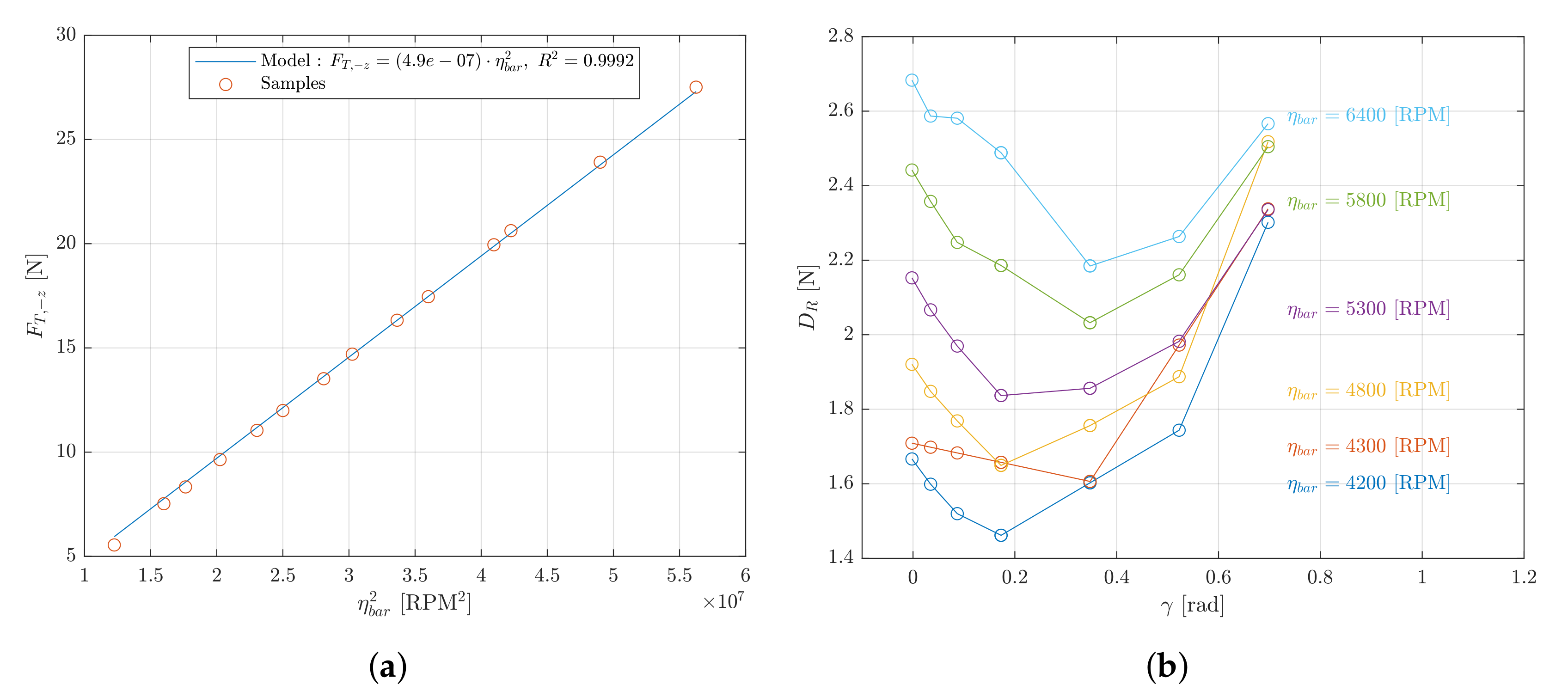
Figure 6.
Model parameters: (a) The thrust model is fitted on data from [28]. Note . (b) Drag model. The wind tunnel drag force model is from [28]. Note .

Figure 7.
Wind estimation for sample hovering flight. The thick blue line represents the ground truth and the other lines represent the estimation methods tested. Shaded areas show two examples of wind gusts (see discussion in Section 4.1.1).
Figure 7.
Wind estimation for sample hovering flight. The thick blue line represents the ground truth and the other lines represent the estimation methods tested. Shaded areas show two examples of wind gusts (see discussion in Section 4.1.1).

Figure 8.
Wind estimation for sample square flight. Thick blue line represents the ground truth and the remaining lines represent the estimation methods tested. The blue highlight shows one occurrence of the tilt estimation failing during an acceleration phase. The red and yellow highlights show two occurrences of non successful estimation of wind (see discussion in Section 4.2).

Figure 9.
Wind estimation for sample vertical flight. Thick blue line represents the ground truth and remaining lines represent estimation methods tested. Blue and red highlights correspond to time intervals in which the drone is ascending and descending, respectively (see discussion in Section 4.3).

Figure 10.
Reference data for sample hovering flight. Thick blue line represents the instantaneous mean of all three reference sensors and the other lines represent each individual sensor. All three highlights show occurrences of high ground truth error (see discussion in Section 5.2.3).
Figure 10.
Reference data for sample hovering flight. Thick blue line represents the instantaneous mean of all three reference sensors and the other lines represent each individual sensor. All three highlights show occurrences of high ground truth error (see discussion in Section 5.2.3).


Table 1.
Most relevant publications using multirotor UAVs to estimate wind (publications on wind estimation for navigation are not included).
Table 1.
Most relevant publications using multirotor UAVs to estimate wind (publications on wind estimation for navigation are not included).
| Year | Author | Method | Data Type | Flight Type | Vert. Wind |
|---|---|---|---|---|---|
| 2015 | Neumann et al. [13] | Tilt | Wind tunnel and Field | Hover and Moving | No |
| 2017 | Palomaki et al. [14] | Tilt | No wind and Field | Hover | No |
| 2018 | Song et al. [15] | Tilt | Wind tunnel | Hover | No |
| 2019 | Xing et al. [16] | Kalman Filtering | Simulation | Hover | No |
| 2019 | Wang et al. [17] | Machine Learning | Wind tunnel | Hover | No |
| 2019 | Perozzi et al. [18] | System Identification | Simulation | Moving | Yes |
| 2019 | Qu et al. [19] | Kalman Filtering | Simulation | Moving | No |
| 2020 | Abichandani et al. [20] | Tilt | Simulation | Hover | No |
| 2020 | González-Rochaz et al. [21] | System Identification | Field | Hover and Vert. Prof. | No |
| 2020 | Allison et al. [22] | Machine Learning | Simulation | Hover | No |
| 2020 | Loubimov et al. [23] | System Identification | Simulation | Hover | No |
Table 2.
UNIS AWS sensor set.
| Sensor Name | Quantity | Accuracy | Frequency | Datasheet |
|---|---|---|---|---|
| Youg 05103 | Wind Speed | 0.3 (m/s) | 1 (Hz) | [31] |
| Youg 05103 | Wind Direction | 3 (deg) | 1 (Hz) | [31] |
| PT1000 | Air Temperature | 0.8 (°C) | 1 (Hz) | [32] |
| Youg 61302L | Air Pressure | 0.3 (hPa) | 1 (Hz) | [33] |
| Rotronic HygroClip | Relative humidity | 0.8 (%) | 1 (Hz) | [34] |
Table 3.
MoTUS sensor set.
| Sensor Name | Quantity | Accuracy | Frequency | Datasheet |
|---|---|---|---|---|
| Gill WindMaster | Wind Speed | 0.01 (m/s) | 10 (Hz) | [35] |
| Gill WindMaster | Wind Direction | 2 (deg) | 10 (Hz) | [35] |
Table 4.
TOPO AWS Sensor set.
| Sensor Name | Quantity | Accuracy | Frequency | Datasheet |
|---|---|---|---|---|
| SparkFun SEN-08942 | Wind Speed | 0.1 (m/s) | 1 (Hz) | [36] |
| SparkFun SEN-08942 | Wind Direction | 22.5 (deg) | 1 (Hz) | [36] |
| Sensirion SHT85 | Air Temperature | 0.1 (°C) | 1 (Hz) | [37] |
| MS5837-02BA | Air Pressure | 2 (hPa) | 1 (Hz) | [38] |
| Sensirion SHT85 | Relative humidity | 1.5 (%) | 1 (Hz) | [37] |
Table 5.
Tilt to air velocity model parameter (see Equation (2)).
Table 5.
Tilt to air velocity model parameter (see Equation (2)).
| Symbol | Value | Unit |
|---|---|---|
| (m/s) | ||
| (m/s) | ||
| (m/s) | ||
| (rad) |
Table 6.
Statistical evaluation of the hover flight shown in Figure 7. The lowpass filter cutoff frequency is 0.1 Hz (see Section 2.4.3).
Table 6.
Statistical evaluation of the hover flight shown in Figure 7. The lowpass filter cutoff frequency is 0.1 Hz (see Section 2.4.3).
| Horizontal Wind (m/s) | Vertical Wind (m/s) | |||||||
|---|---|---|---|---|---|---|---|---|
| Not Filtered | Lowpass Filtered | Not Filtered | Lowpass Filtered | |||||
| Bias | Std | Bias | Std | Bias | Std | Bias | Std | |
| DM, Linear and No Vertical Drag | 0.46 | 1.08 | 0.46 | 0.84 | 0.04 | 0.50 | 0.04 | 0.44 |
| DM, Linear and Vertical Drag | 0.29 | 1.07 | 0.29 | 0.82 | 1.53 | 0.82 | 1.53 | 0.68 |
| DM, Quadratic and No Vertical Drag | 1.90 | 1.78 | 1.89 | 1.25 | 0.04 | 0.50 | 0.04 | 0.44 |
| DM, Quadratic and Vertical Drag | 1.42 | 1.75 | 1.42 | 1.17 | 2.25 | 0.98 | 2.25 | 0.79 |
| Tilt | 0.15 | 0.93 | 0.15 | 0.70 | 0.04 | 0.50 | 0.04 | 0.44 |
Table 7.
Statistical evaluation of the square flight shown in Figure 8. The lowpass filter cutoff frequency is 0.1 Hz (see Section 2.4.3).
Table 7.
Statistical evaluation of the square flight shown in Figure 8. The lowpass filter cutoff frequency is 0.1 Hz (see Section 2.4.3).
| Horizontal Wind (m/s) | Vertical Wind (m/s) | |||||||
|---|---|---|---|---|---|---|---|---|
| Not Filtered | Lowpass Filtered | Not Filtered | Lowpass Filtered | |||||
| Bias | Std | Bias | Std | Bias | Std | Bias | Std | |
| DM, Linear and No Vertical Drag | 0.93 | 1.84 | 0.90 | 1.32 | 0.46 | 0.54 | 0.46 | 0.46 |
| DM, Linear and Vertical Drag | 0.69 | 1.68 | 0.68 | 1.09 | 1.42 | 1.55 | 1.40 | 0.92 |
| DM, Quadratic and No Vertical Drag | 1.51 | 2.47 | 1.50 | 1.64 | 0.46 | 0.54 | 0.46 | 0.46 |
| DM, Quadratic and Vertical Drag | 1.14 | 2.31 | 1.14 | 1.44 | 1.90 | 1.42 | 1.87 | 0.80 |
| Tilt | 0.40 | 7.94 | 0.39 | 4.34 | 0.46 | 0.54 | 0.46 | 0.46 |
Table 8.
Statistical evaluation of the vertical flight shown in Figure 9. The statistics are evaluated only during the ascension phases of the flight. The lowpass filter cutoff frequency is 0.1 Hz (see Section 2.4.3).
Table 8.
Statistical evaluation of the vertical flight shown in Figure 9. The statistics are evaluated only during the ascension phases of the flight. The lowpass filter cutoff frequency is 0.1 Hz (see Section 2.4.3).
| Horizontal Wind (m/s) | Vertical Wind (m/s) | |||||||
|---|---|---|---|---|---|---|---|---|
| Not Filtered | Lowpass Filtered | Not Filtered | Lowpass Filtered | |||||
| Bias | Std | Bias | Std | Bias | Std | Bias | Std | |
| DM, Linear and No Vertical Drag | 0.44 | 0.95 | 0.38 | 0.59 | 0.05 | 0.33 | 0.03 | 0.26 |
| DM, Linear and Vertical Drag | 0.66 | 0.82 | 0.59 | 0.52 | 0.28 | 0.67 | 0.36 | 0.31 |
| DM, Quadratic and No Vertical Drag | 1.18 | 1.70 | 1.20 | 1.00 | 0.05 | 0.33 | 0.03 | 0.26 |
| DM, Quadratic and Vertical Drag | 0.53 | 1.22 | 0.51 | 0.78 | 0.78 | 1.00 | 0.43 | 0.51 |
| Tilt | 0.73 | 0.93 | 0.63 | 0.57 | 0.05 | 0.33 | 0.03 | 0.26 |
Table 9.
Statistical evaluation of the reference data of the flight shown in Figure 7.
Table 9.
Statistical evaluation of the reference data of the flight shown in Figure 7.
| Horizontal Wind | Vertical Wind | |||||||
|---|---|---|---|---|---|---|---|---|
| Not Filtered | Lowpass Filtered | Not Filtered | Lowpass Filtered | |||||
| Bias | Std | Bias | Std | Bias | Std | Bias | Std | |
| Sensor at 21.3 (m) | 0.21 | 0.61 | 0.21 | 0.43 | 0.04 | 0.37 | 0.04 | 0.25 |
| Sensor at 18.0 (m) | 0.19 | 0.49 | 0.19 | 0.27 | 0.00 | 0.30 | 0.00 | 0.15 |
| Sensor at 14.7 (m) | 0.13 | 0.62 | 0.13 | 0.44 | 0.04 | 0.39 | 0.04 | 0.27 |
Table 10.
Statistical evaluation of the hover flight presented in Table 6 compared with statistical evaluation of Test 4 described in Table 2 of [8]. Note, in the latter, sampling frequency is 20 Hz whereas this work uses 10 Hz.
| Horizontal Wind (m/s) | Vertical Wind (m/s) | |||||||
|---|---|---|---|---|---|---|---|---|
| Not Filtered | Lowpass Filtered | Not Filtered | Lowpass Filtered | |||||
| Bias | Std | Bias | Std | Bias | Std | Bias | Std | |
| DM, Linear and No Vertical Drag | 0.46 | 1.08 | 0.46 | 0.84 | 0.04 | 0.50 | 0.04 | 0.44 |
| Tilt | 0.15 | 0.93 | 0.15 | 0.70 | 0.04 | 0.50 | 0.04 | 0.44 |
| On-board flow sensor [8] | 0.2 | 0.23 | N/A | N/A | 0.02 | 0.05 | N/A | N/A |
Publisher’s Note: MDPI stays neutral with regard to jurisdictional claims in published maps and institutional affiliations. |
© 2022 by the authors. Licensee MDPI, Basel, Switzerland. This article is an open access article distributed under the terms and conditions of the Creative Commons Attribution (CC BY) license (https://creativecommons.org/licenses/by/4.0/).
Share and Cite
MDPI and ACS Style
Meier, K.; Hann, R.; Skaloud, J.; Garreau, A. Wind Estimation with Multirotor UAVs. Atmosphere 2022, 13, 551. https://0-doi-org.brum.beds.ac.uk/10.3390/atmos13040551
AMA Style
Meier K, Hann R, Skaloud J, Garreau A. Wind Estimation with Multirotor UAVs. Atmosphere. 2022; 13(4):551. https://0-doi-org.brum.beds.ac.uk/10.3390/atmos13040551
Chicago/Turabian StyleMeier, Kilian, Richard Hann, Jan Skaloud, and Arthur Garreau. 2022. "Wind Estimation with Multirotor UAVs" Atmosphere 13, no. 4: 551. https://0-doi-org.brum.beds.ac.uk/10.3390/atmos13040551
Note that from the first issue of 2016, this journal uses article numbers instead of page numbers. See further details here.