
Assessment of the Performance of a Low-Cost Air Quality Monitor in an Indoor Environment through Different Calibration Models


Brindisi Research Center, Department for Sustainability, ENEA—Italian National Agency for New Technologies, Energy and Sustainable Economic Development, SS. 7, Appia, km 706, 72100 Brindisi, Italy
*
Author to whom correspondence should be addressed.
Atmosphere 2022, 13(4), 567; https://0-doi-org.brum.beds.ac.uk/10.3390/atmos13040567
Submission received: 8 February 2022
/
Revised: 15 March 2022
/
Accepted: 30 March 2022
/
Published: 31 March 2022
(This article belongs to the Special Issue State-of-Art in Real-Time Air Quality Monitoring through Low-Cost Technologies)
Abstract
:Air pollution significantly affects public health in many countries. In particular, indoor air quality can be equally, if not more, concerning than outdoor emissions of pollutant gases. However, monitoring the air quality in homes and apartments using chemical analyzers may be not affordable for households due to their high costs and logistical issues. Therefore, a new alternative is represented by low-cost air quality monitors (AQMs) based on low-cost gas sensors (LCSs), but scientific literature reports some limitations and issues concerning the quality of the measurements performed by these devices. It is proven that AQM performance is significantly affected by the calibration model used for calibrating LCSs in outdoor environments, but similar investigations in homes or apartments are quite rare. In this work, the assessment of an AQM based on electrochemical sensors for CO, NO2, and O3 has been performed through an experiment carried out in an apartment occupied by a family of four during their everyday life. The state-of-the-art of the LCS calibration is featured by the use of multivariate linear regression (MLR), random forest regression (RF), support vector machines (SVM), and artificial neural networks (ANN). In this study, we have conducted a comparison of these calibration models by using different sets of predictors through reference measurements to investigate possible differences in AQM performance. We have found a good agreement between measurements performed by AQM and data reported by the reference in the case of CO and NO2 calibrated using MLR (R2 = 0.918 for CO, and R2 = 0.890 for NO2), RF (R2 = 0.912 for CO, and R2 = 0.697 for NO2), and ANN (R2 = 0.924 for CO, and R2 = 0.809 for NO2).
1. Introduction
Air pollution represents one of the main concerns for public health in almost every country around the globe. It is proven that this issue is the cause of premature death for seven million people annually [1]. The European Commission has also shown that European citizens spend around the 90% of their time in indoor environments, mainly at home or in workplaces [2]. For this reason, the indoor environment can drastically affect people’s health, positively or negatively. Another study conducted by the US Environmental Protection Agency (EPA) has shown that indoor environments can be two to five times more toxic than outdoor locations [3]. Therefore, it is clear that air quality monitoring in indoor environments is needed for the personal exposure risk assessment of air pollutants. Currently, air quality monitoring is performed by government authorities through the use of chemical analyzers, which are bulky, heavy, and require routine maintenance. In addition, they are also very expensive (their prices ranges between EUR5000 and EUR30,000) [4,5], thus, they hardly can be afforded by households and common citizens.
In recent years, the use of air quality monitors (AQMs) based on low-cost gas sensors (LCSs) has become more and more popular, due to their affordability, portability, and ease of use [5,6,7]. The working principles of LCSs, on which AQMs are based, are comprised by different technologies that provide several advantages, such as low power consumption, device compactness, and little need for maintenance. The use of LCSs was tested, not only for air quality assessment, but also for other real-world applications, such as malodor detection [8,9].
A key factor determining the performance of LCS sensors and AQMs based on them is represented by the algorithm, or the calibration model, used for their calibration [5]. The linear regression (LR) and the multivariate linear regression (MLR) methods, along with several machine learning models, are the most frequently used.
Concerning the particulate matter (PM) concentration measurement, LCSs based on laser light scattering are currently employed worldwide, and their performance has been investigated in several studies. For example, Si and others [10] tested four different calibration models to evaluate the performance of the PMS5003 sensor. They compared the results given by the LR, MLR, and other machine learning algorithms, such as XGBoost, and the artificial feedforward neural network (ANN). The authors of this study found that the most promising method to obtain good quality data from the PMS5003 sensor in an outdoor environment is represented by the feedforward ANN. Other examples of machine learning calibration models employed for LCS calibration can be found in [11].
Regarding LCSs for measuring pollutant gases, if we consider their advantages, they look to be the ideal substitute for chemical analyzers, but unfortunately, they cannot offer the same accuracy level, and the data produced by such devices have not always proved reliable [4,5,6,7]. In fact, LCSs, and therefore AQMs, are sensitive to temperature and humidity changes; moreover, they suffer from drift phenomena. These factors are the origin of inaccuracies in measurements and may lead to the deterioration of AQM performance. In addition to these elements, it has to be considered that in general, LCSs may not be selective; this means that measurements performed by sensors designed for carbon monoxide, for example, can be affected by the presence of other gases (called interfering gases) which can alter the correct measurement of carbon monoxide concentrations. This effect is also known as sensor cross-sensitivity.
To account for these adverse factors, researchers have found that the adoption of advanced calibration techniques can significantly improve AQM performance. They have also found that the most effective way to maximize their performance in real-world applications is to calibrate them in co-location with reference instruments placed in the final deployment environment.
The most common calibration algorithms for LCSs used in the recent studies are based on multivariate linear regression (MLR), support vector regression (SVR), random forest regression (RF), and artificial neural networks (ANN).
In any case, the current research on LCS calibration does not provide clear indications about which calibration approach achieves the best AQM performance, but previous studies seem to indicate that the reliability of data produced by AQMs also depends on the environmental variables [4]. More specifically, the LCS calibration process can be affected by the combination of concentration levels of target gases, the variability range of temperature and humidity, and the concentration levels of interfering gases [4].
In this respect, a consistent number of studies have been conducted to explore the performance of calibration algorithms in outdoor environments featuring different conditions; on the contrary, very few investigations (to the best of our knowledge) have been performed to assess the effectiveness of such techniques in an indoor, real-world scenario using the co-location of reference instruments with the AQM in question.
Castell et al. [4] highlighted that a good performance of AQMs in the laboratory is not indicative of good performance in real-world scenarios. In this study, CO, NO, O3, and NO2 LCSs were calibrated by using linear regression (LR) models in outdoor environments. However, it must be noted that, concerning the state-of-the-art of calibration models, the most widely used method to calibrate LCSs is the multivariate linear regression (MLR) [5]. Other approaches for AQM calibrations are the random forest (RF) algorithm, the support vector machine (SVM), and artificial neural networks (ANN) [5].
Several works tested these calibration models in an outdoor environment, reporting various results in terms of performance quality. In this study, we focused our investigation on the electrochemical LCSs, neglecting of the scope other types of air pollutant sensors. In Table 1, data from previous studies are summarized to provide an indication of the results achieved in outdoor environment using the previously mentioned models to calibrate AQMs or LCSs.
Concerning the use of AQMs based on LCSs in indoor environments, some studies were conducted to explore their potentialities and capabilities. In one of these studies, Pitarma and others [19] proposed a wireless sensor network system for monitoring CO and CO2 concentrations, along with other environmental parameters. In the work of Zhang [20], a wider range of air pollutants was monitored through a custom-built monitoring system capable of detecting TVOCs (total volatile organic compounds), CO, CO2, NO2, SO2, O3, PM10, PM2.5, and PM1. An IoT (Internet of Things) based air quality monitoring platform called “Smart-Air” was presented by Byung Wan Jo [21] for measuring VOC, CO, and CO2. This system was implemented in the Hanyang University of Korea to demonstrate its feasibility. However, all these studies were conducted without comparing the performance of AQMs in co-location with reference instrumentation to provide an idea of the effective quality of the data produced by them. Moreover, no information was provided about the LCS calibration algorithms used in the AQMs. Few studies involving LCSs in co-location with reference instruments to test AQM data reliability in an indoor environment were conducted. Most studies are focused on investigating the use of AQMs for PM, TVOC, and CO2 concentration measurements [22,23,24]. To the best of our knowledge, only Tryner and Volckens et al. [25] measured indoor CO, NO2, and O3 concentrations, testing these in a kitchen of an occupied home in co-location with reference monitors. The calibration algorithm used in this study was the MLR, while the total duration of the experiment was 168 h.
The previous studies involving AQMs based on LCSs have proven that AQM data quality significantly depends on the calibration algorithm used, on the concentration levels of the target gases, and on the variability of the interfering parameters, such as temperature, humidity, and the interfering air pollutants. All these factors, in conjunction with the lack of studies comparing CO, NO2, and O3 sensor performance with reference monitors in an indoor environment, have induced us to explore the variation of the performance of these LCSs by using different calibration algorithms in an indoor experiment. Therefore, to accomplish this objective, an AQM designed and developed in our laboratories has been placed in co-location with reference monitors in an occupied home for measuring NO2, CO, and O3 concentrations during everyday life. The experiment enabled us to compare the performance of electrochemical CO, NO2, and O3 sensors by using different calibration algorithms such as MLR, RF, SVM, and ANN (see Section 2.3 for more details).
2. Materials and Methods
2.1. The Experimental Setup
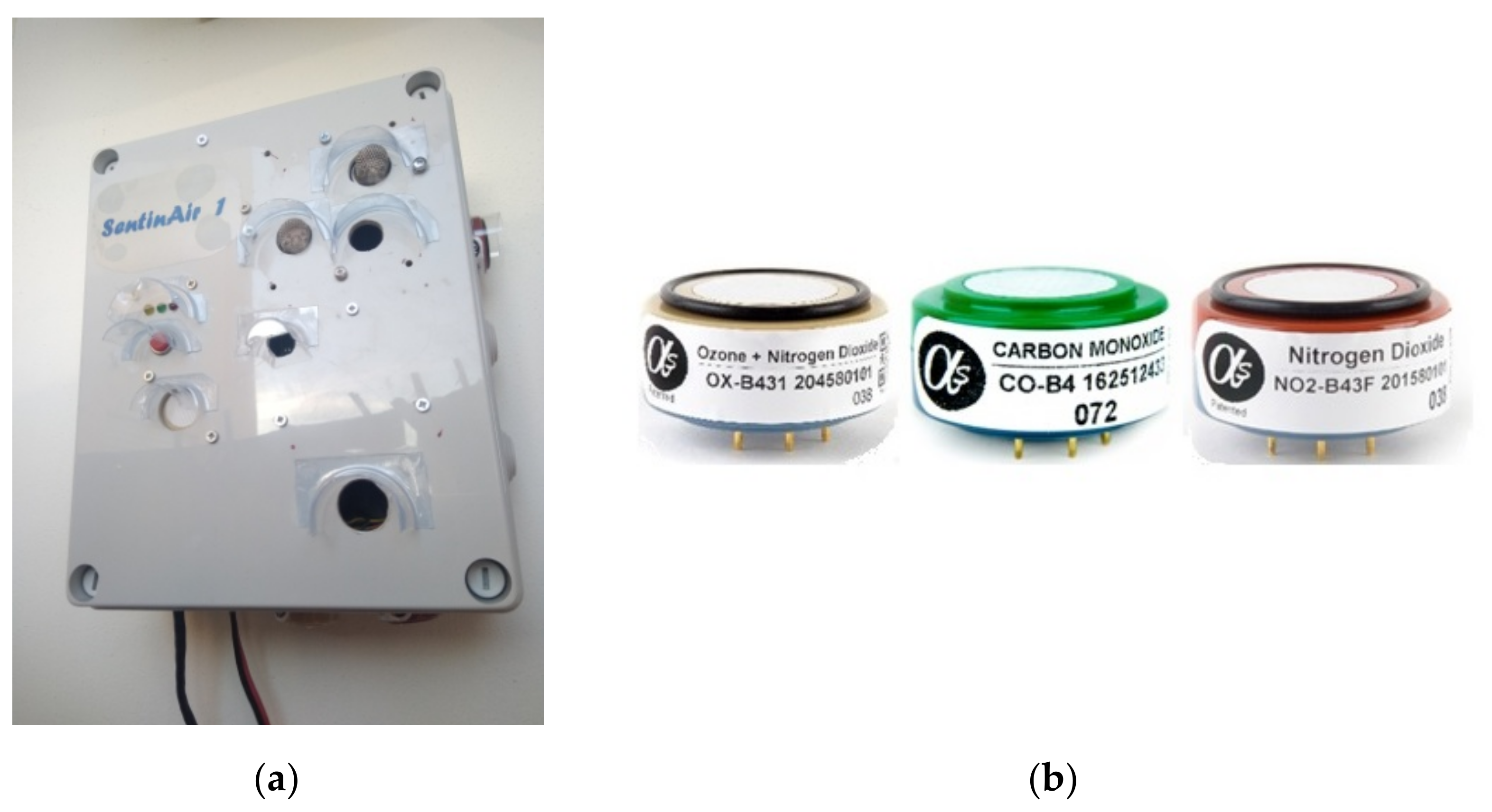
The AQM used for this experiment, called SentinAir (see Figure 1a), was designed and developed in the laboratories of the ENEA research center of Brindisi (Italy) by D. Suriano, and it is capable of being used with different LCS types [15]. Previous articles [15,26,27] have been described in detail the SentinAir system, while all the information and the materials needed to assemble it can be found in online repositories [28,29,30]. For each air pollutant, two LCSs have been used during the experiment (see Figure 1b); they have been assembled in the SentinAir AQM along with the temperature and relative humidity (RH) sensors. In Table 2, information about the LCSs used for this study is reported, along with the target gas they are designed to test. All the LCSs involved in the experiment are four-electrode electrochemical gas sensors designed for ppb gas levels. In addition to the standard working, reference, and counter electrodes, a fourth auxiliary electrode is used to correct for zero current changes. Therefore, each sensor provides two output signals: the working, and the auxiliary electric current. The manufacturer suggests subtracting the auxiliary signal from the working one, considering the sensor output as their difference. The weak continuous current provided by these sensors (see Table 2) must be converted into a voltage signal, which in turn, must be converted into digital data, following the scheme depicted in Figure 2.
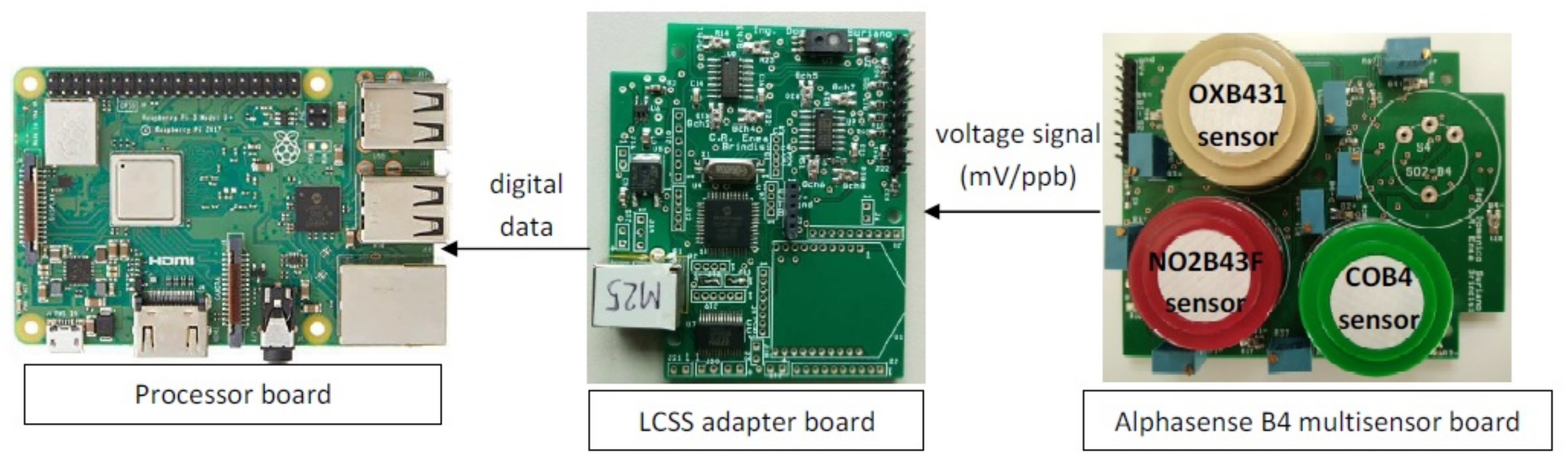
Sensors must be mounted on an electronic support board for their operation. The sensor manufacturer provides such boards, but their output sensitivity cannot be set by the customer after their purchase. For this reason, we decided to design and implement in our laboratory an electronic board (the Alphasense B4 multisensor board designed by D. Suriano in the ENEA research center of Brindisi in Italy) suitable for our purposes. All the information and details for assembling it, along with those related to the LCSS adapter board shown in Figure 2, can be found in [15,26,27,28,29,30]. The sensitivity parameters at the support board output (here expressed in mV/ppb) related to each sensor, along with low electric noise, could have a significant impact on the sensor performance; therefore, in LCS performance assessment studies, it could be very useful to know these, but unfortunately, they are very often not reported. The theoretical values of sensitivity for each sensor used in the experiment are shown in Table 3. They are calculated using the amplification gain of the electronic circuits featured in the Alphasense B4 multisensor board and the resistive values of the variable resistors mounted on it (see [30] for further details).
The reference instrumentation used for the experiment were the 106L GO3 PRO model for ozone measurements [34], the 405 nm NO2/NO/NOx monitor [34], and the CO12 model for carbon monoxide measurements by Envea [35]. The SentinAir system is capable of automatically connecting with these instruments, thus it was possible to synchronously read data emitted by them and LCS signals (see [15,26,27,28]).
2.2. The Experiment Location
This study was conducted in an occupied apartment located in Mesagne, a town in the south of Italy. A maximum number of four people were in the apartment at various hours of the day, while ordinary activities and events occurred during the usual daily routine. Cooking food using the gas burner stove, smoking tobacco, using the laser printer, burning candles, etc., produced different concentrations of CO, NO2, and O3. As the aim of this study is not focused on relating gas concentration levels to a particular type of source, the time of the different events was not systematically logged, but some indications are provided in correspondence with the most significant events. The apartment is composed of the daytime area and the nighttime area, separated by a door. The experimental setup was placed in the daytime area (see Figure 3b), while the door separating the living room from the nighttime area was kept closed throughout the duration of the experiment. This precaution was necessary to limit the effects of the permanent buzzing sound produced by the reference monitors during their operation.
2.3. The Calibration Algorithms
By examining the scientific literature, it appears that the most used calibration techniques for AQM calibration are based on LR, MLR, RF, SVM, and ANN algorithms (at least, in outdoor environments) [5]. Considering that the best performance has always been achieved by MLR, RF, SVM, or ANN, we decided to exclude the LR approach from our investigation. MLR is the most widely used calibration algorithm [5]; it consists of a linear function structured as in Equation (1), where y is the regressor, x1, x2, xn are the predictors, and the αi coefficients are calculated by using the ordinary least square method.
The RF calibration model is a machine learning algorithm for solving regression or classification problems [36]. It constructs an ensemble of decision trees using a training dataset; thus, the mean value from that ensemble is used to predict the value for new input data.
The SVM solves a regression problem in three main steps: first, the input data are mapped into a feature space employing a kernel function; then, the flattest function fitting the input images is found by solving the corresponding constrained optimization equation. Support vectors are the points corresponding to the non-null Lagrangian multipliers of this latter function. In the last step, the results are mapped back into the input space [37]. ANNs are very sophisticated techniques able to model very complex functions through artificial units, the neurons, arranged in various architectures. Among the various ANN types, we considered the multilayer perceptron (MLP) [38] for this study, due to its successful application in previous works [16,17]. The MLP architecture generally arranges the neurons in more layers: the input layer includes the neurons where inputs are applied; thus, the output of this layer acts as the input for the next one, and so on, until the final output layer. This last layer provides the output final data. One or more layers, called hidden layers, can be located in the midst of the input and output layers, depending on the MLP architecture adopted. There is no well-defined procedure for precisely identifying the number of neurons and layers for the optimal performance; rather, empirical methods featured by trial-and-error mechanisms are often used for their selection.
The software used for the implementation of the calibration algorithm was the open-source Scikit-learn library [39,40,41]. Employing this resource, RF and SVM parameter tuning was performed to select the optimal configuration for these machine learning algorithms (see also the Supplementary Materials, Listing S1). Concerning the MLP, over 10000 types were tested to find the optimal solution. Architectures with one or two hidden layers were tested, while the number of neurons for each layer ranged from 10 to 200. For the MLP training, the BFGS algorithm was used [42], while input data were previously scaled by applying a transformation with a means of zero and variance of 1.
Unlike some previous studies, we selected predictor variables uniquely related to sensor outputs, avoiding using data coming from reference devices, in order to assess AQM use potentiality in real-world applications without relying on reference instruments that are not always available.
Moreover, the sensor manufacturer and some previous works consider the difference between working and auxiliary electrode signals as the sensor output; therefore, this is used as a predictor in the calibration models. In this study, we considered two sets of predictor variables for each group of sensors: the first one is composed of temperature, relative humidity, and the signals of the working and auxiliary electrodes of sensors involved in the elaboration, while the second one (hereafter denoted with the suffix “net”) is formed by the temperature, relative humidity, and the difference between the working and auxiliary electrodes of each sensor. The calculations carried out through each calibration model used in this experiment were performed by using both the two predictor sets as input, in order to investigate if these two optional approaches originate significant differences in terms of AQM pollutant concentration prediction capability.
Finally, as a criterion followed in selecting predictor variables, we considered the data related to interfering gas for each sensor, as provided by the manufacturer. By examining these, it can be seen that the COB4 output is not significantly affected by NO2 and O3 concentrations, while the NO2B43F is provided with an ozone filter which limits its cross-sensitivity for this gas. On the contrary, the OXB431 sensor detects both ozone and nitrogen dioxide; therefore, for ozone concentration prediction, we also included NO2B43F sensor outputs as predictors. As suggested by the manufacturer, to take into account the effect of the NO2 cross-sensitivity, we considered as predictors the difference between the OXB431 and the NO2B43F sensor outputs (see Table 4).
Finally, considering that we have two groups of sensors—hereafter marked with (1) and (2)—and two sets of predictors for each pollutant gas, in total, there will be four sets of predictors to set as input for each model considered in this study. In Table 4, the complete sets of predictor variables selected for our investigation are summarized.
2.4. Model Evaluation and Metrics
The dataset collected during the experiment was split into two parts: the part related to the first period of the experiment was used for LCS calibration, while the second part was used for validation. The metrics adopted for both the calibration and validation processes were the coefficient of determination (R2), the mean absolute error (MAE), the root mean squared error (RMSE), and the normalized root mean squared error (nRMSE), defined in Equations (2)–(5).
In the above equations, N is the number of records belonging to the dataset, mi represents the i-th value given by the model, ri is the reading of the reference instrument, is the average of the reference readings, while represents the average of measurements given by the model.
The coefficient of determination ranges from 0 to 1 and gives us an idea about how accurately the AQM measurements follow the reference readings, or in other words, the grade of correlation between AQM and reference data. Values close to 1 indicate good performance; on the contrary, if the values are near 0, it means a poor correlation. MAE and RMSE are both indicators that provide information about the entity of the error between the model and the reference. Lower values underline better performances. The nRMSE indicator is necessary for allowing us to make a comparison of the performance given by the models for different pollutant gases. Even in this case, nRMSE values close to 0 suggest good performance.
3. Results
The experiment lasted 186 h and 54 min, producing a dataset featured by a total number of 5607 records, taken at a sampling rate of 2 min. The calibration dataset includes data recorded from 13 December 2021 to 17 December 2021, providing 2575 records; the validation dataset includes readings from 17 December 2021 to 21 December 2021, resulting in 3032 records.
CO, NO2, and O3 concentration statistics, as monitored by the reference during the calibration and validation period, are summarized in Figure 4a, while in Figure 4b, the temperature and relative humidity ranges are shown. Data related to these last two parameters were obtained from the sensors mounted inside the AQM and placed very close (less than 10 cm) to the LCSs. For this reason, they were able to measure the values actually experienced by the sensors rather than the values related to the room where the AQM was placed.
Model evaluations based on the metrics selected for their assessment are revealed in Table 5. By examining this table, we see that, if we consider the coefficient of determination (R2) and the validation dataset, the best performance related to CO, NO2, and O3 is respectively achieved by the CO(2) predictor set calibrated through ANN, by the NO2(1) calibrated through MLR, and the O3(1) calibrated by MLR.
Time series and scatter-plots referring to the previously mentioned three cases are shown in Figure 5, Figure 6, Figure 7, Figure 8 and Figure 9. In particular, Figure 5 shows the time series related to the calibration dataset, while in Figure 6, it is possible to see the data concerning the validation dataset. In these figures, some events originating the pollutant gases are reported for an indicative idea about the possible sources of domestic pollution. During the experiment, a systematic logging of every event related to the monitored pollutant gases was not carried out, because the aim of this study is mainly focused on assessing the AQM performance calibrated by different models. Figure 5 reports the predictions during the calibration period described for CO (Figure 5a), NO2 (Figure 5b), and O3 (Figure 5c). These are featured by a coefficient of determination of 0.975, 0.734, and 0.432, respectively. Similarly to Figure 5, data reported in Figure 6 are related to the validation period for CO (Figure 6a), NO2 (Figure 6b), and O3 (Figure 6c). The coefficient of determination in these three cases is respectively 0.924, 0.890, and 0.137.
To better understand the differences in prediction capability of the AQM by using the calibration models under investigation, it is useful to analyze Table 6 and Table 7. In these tables, the median values of R2 and nRMSE are reported for each model by separately considering the three pollutants. In particular, by taking into account the median values and not the best ones, Table 7 shows that, in terms of R2, ANN achieves the best performance in predicting the CO concentrations, while for NO2 and O3, the MLR model offers the best results. As expected, values related to the calibration dataset shown in Table 6 are in general better than the respective values shown in Table 7, where calculations performed by the validation dataset are shown.
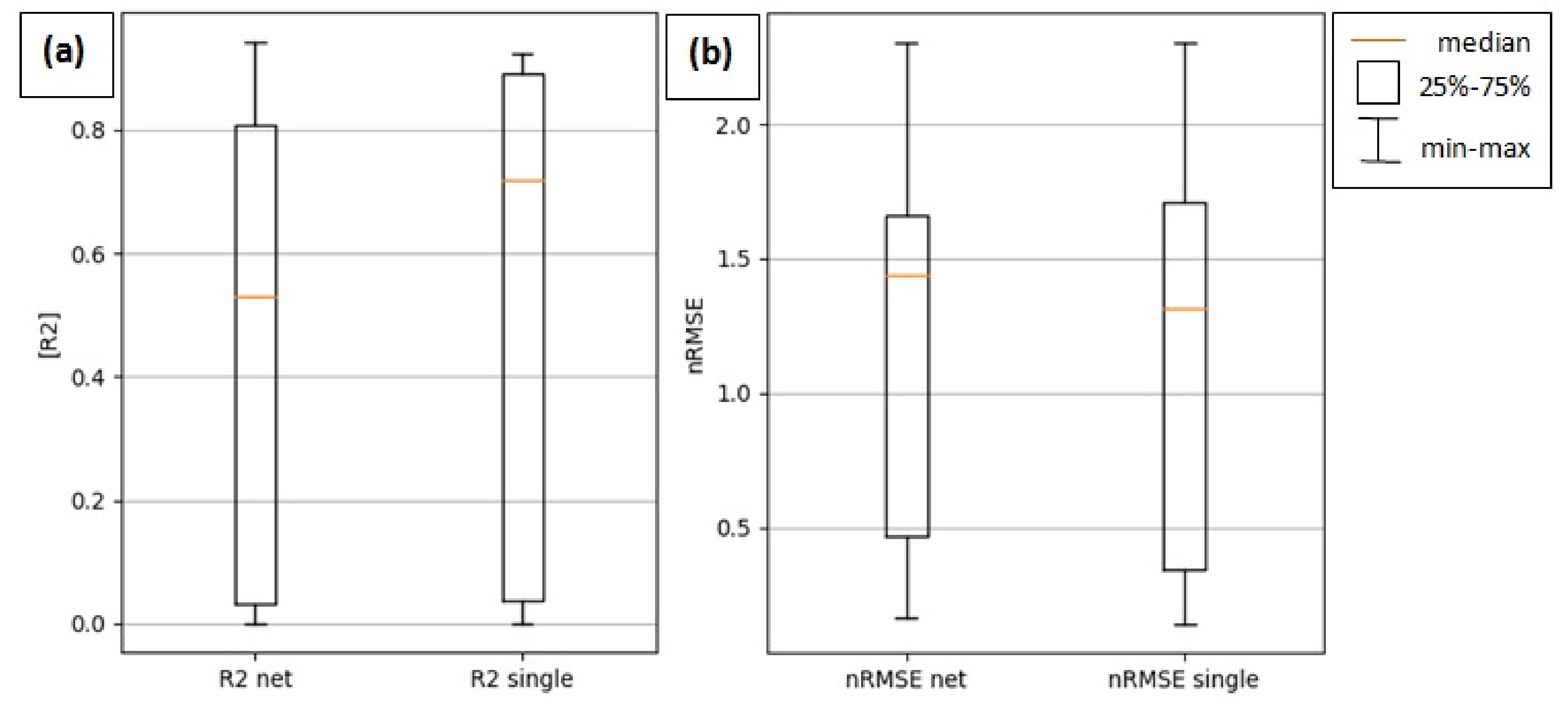
In this experiment, we decided to investigate the effects of different inputs or predictors for MLR, RF, SVM, and ANN calibration models (see Table 4). These inputs can be distinguished into two subsets. The first subset is defined by taking as a predictor the difference between the “working” and “auxiliary” electrodes of each sensor selected for predicting the gas concentrations. The second subset includes the sets where a predictor variable is represented by every single electrode of the sensor (see Table 4). The results obtained by comparing the performance achievable through the two subsets and considering all the calibration models related to CO, NO2, and O3 are reported in Figure 10. The indicators used for this analysis are represented by R2 and nRMSE, while the results originated by the first subset are marked with the “net” suffix, and the results from the second subset are denoted by the “single” suffix.
4. Discussion
By analyzing Table 5 and Table 7, it can be seen that the best performance related to the validation dataset was achieved for CO and NO2 predictions, while all the indicators show that the poorest performance was for the O3 measurements. This result is further highlighted by the scatter plots shown in Figure 9, where the spread of point clouds indicates the low correlation between the predicted ozone concentrations and those measured by the reference. One possible explanation can be provided by the high cross-sensitivity of ozone sensors to NO2 concentrations. If we carefully inspect Figure 5 and Figure 6, it can be noted that NO2 emissions are almost always originated in concurrence with ozone production. This element, in conjunction with a lower range of ozone concentrations compared with the NO2 levels, shown in Figure 4, could explain this relevant difference between the ozone concentration prediction and the other results. Moreover, by inspecting Figure 4b, it can be seen that the temperature and relative humidity levels experienced by the sensors under test mostly fall into a relatively restrained range. This factor has contributed to limit the interfering effects of these two parameters, ending up benefiting the overall LCS performance.
If we want to try a comparison with similar previous works, we must distinguish between studies carried out in outdoor environments and indoor investigations performed in an occupied home. While the first category of works is characterized by a relevant number of studies (see the review written by Karagulian et al. [5]), to the best of our knowledge, the only study performing AQM data quality assessment by comparison with reference monitors for CO, NO2, and O3 is provided in Tryner’s work [25], although this study was carried out through a test methodology different from the approach followed here. In any case, some similarities can be found by comparing the two experiments: in general, CO, and NO2 predictions are more accurate than the ozone predictions, and in particular, CO measurements exhibit more correlation with the reference data. The indicators used for both the studies were R2, MAE, and RMSE, allowing us to build Table 8, where the median values of the indicators summarize the differences found between that study and our current research.
Concerning the investigations carried out in outdoor environments, we can refer to the work of Karagulian [5], which also provides data related to the calibration model used in the various studies. The comparison between this work and the previously mentioned studies is exposed in Table 9, where it can be noted that data related to CO and NO2 are quite comparable, except for in the SVM case. On the contrary, results concerning the O3 pollutant significantly differ from the data found in this experiment. A possible explanation could be that LCS performance is significantly sensitive to both the gas concentration levels and the magnitude of interfering gas concentrations. These two factors can be remarkably different from one environment, or location, to another, causing discrepancies in AQM performance.
Another aspect concerning AQM performance assessment is represented by the model selected for LCS calibration. In this study, we have investigated four calibration models (MLR, RF, SVM, and ANN) utilizing R2, MAE, RMSE, and nRMSE indicators. By examining Table 5, Table 6 and Table 7, it can be noted that, in general, the best performance is achieved by MLR, RF, and ANN models, but also that the data does not clearly indicate the presence of a specific outperforming algorithm. Rather, our analysis suggests that in most cases, the SVM approach provides less accurate predictions for each monitored pollutant. This last element is possibly due to the intrinsic difficulty in finding the optimal model hyperparameter set. The computing time required for determining the optimal hyperparameter combination was significantly larger compared to the that one for other models, and perhaps more extensive efforts and trials would be needed to find them. Finally, it must be noted that fast and optimal hyperparameter tuning is an active research area within the scientific community [14]. However, by assessing those results from a practical point of view, MLR models are much easier to implement using electronic microprocessor boards of AQMs, requiring fewer computational resources. On the contrary, RF and ANN models require more computational power, memory, and dedicated software libraries.
Finally, another aspect investigated through this experiment is represented by the selection of predictors for the calibration models. Figure 10 clearly shows that, taken separately, the “working” and the “auxiliary” signals in the predictor sets generally lead to better performance. This conclusion can be drawn by noting that the median values of R2 and nRMSE shown in Figure 10 are always better in this case, as compared to the “net” predictor choice.
5. Conclusions
The experiment carried out in this work clearly points out that CO, NO2, and O3 pollution can be an issue equally, if not more, concerning than the outdoor emissions of these gases. Monitoring this pollutant by chemical analyzers is not feasible for households, due to their high costs and logistic issues. Moreover, the permanent buzzing sound they usually generate during their operation could be a problem for their use in homes and apartments. An option for addressing these issues could be represented by AQMs based on LCSs, which are significantly less expensive and not noisy.
An experiment was conducted in an occupied home to demonstrate the effectiveness of the AQM for monitoring CO, NO2, and O3 pollutants by using different calibration models. We found that CO and NO2 pollutant concentration measurements are in good agreement with the reference instruments data, if calibrated through MLR, RF, and ANN models. In particular, by considering the validation period, the best performance in terms of R2 for CO concentration measurements was achieved through the ANN model (R2 = 0.924), while the best MAE and RMSE values were achieved by MLR calibration (MAE = 0.099 ppm; RMSE = 0.140 ppm). Moreover, in the case of the NO2, we found that in the validation period, the best performance was given by the MLR model (R2 = 0.924; MAE = 8.381 ppb; RMSE = 10.618 ppb).
Moreover, we proved that model prediction capabilities could be further optimized by separately using sensor electrode signals as inputs.
Supplementary Materials
The following supporting information can be downloaded at: https://0-www-mdpi-com.brum.beds.ac.uk/article/10.3390/atmos13040567/s1, Listing S1: Hyperparameters of RF, SVM, and ANN models used in the experiment.
Author Contributions
Conceptualization, D.S.; methodology, D.S.; software, D.S.; hardware, D.S.; validation, D.S.; formal analysis, D.S.; investigation, D.S.; resources, D.S.; data analysis, D.S.; data curation, D.S.; writing—original draft preparation, D.S.; writing—review and editing, D.S.; visualization, D.S.; supervision, D.S.; experiment design, D.S.; experimental setup preparation, D.S.; funding acquisition, M.P. All authors have read and agreed to the published version of the manuscript.
Funding
This research received no external funding.
Institutional Review Board Statement
Not applicable.
Informed Consent Statement
Informed consent was obtained from all subjects.
Data Availability Statement
The data presented in this work are available on request from the corresponding author.
Acknowledgments
A special thanks to Mattia Suriano, Roberta Suriano, and Marinella Mucci, who patiently supported the experiment’s success.
Conflicts of Interest
The authors declare no conflict of interest.
References
- WHO. How Air Pollution Is Destroying Our Health. 2018. Available online: https://www.who.int/news-room/spotlight/how-air-pollution-is-destroying-our-health (accessed on 7 February 2022).
- European Commission. Indoor Air Pollution: New EU Research Reveals Higher Risks than Previously Thought. 2017. Available online: https://ec.europa.eu/commission/presscorner/detail/en/IP_03_1278 (accessed on 7 February 2022).
- EPA. The Inside Story: A Guide to Indoor Air Quality. 2017. Available online: https://www.epa.gov/indoor-air-quality-iaq/inside-story-guide-indoor-air-quality (accessed on 7 February 2022).
- Castell, N.; Dauge, F.R.; Schneider, P.; Vogt, M.; Lerner, U.; Fishbain, B.; Broday, D.; Bartonova, A. Can commercial low-cost sensor platforms contribute to air quality monitoring and exposure estimates? Environ. Int. 2017, 99, 293–302. [Google Scholar] [CrossRef] [PubMed]
- Karagulian, F.; Barbiere, M.; Kotsev, A.; Spinelle, L.; Gerboles, M.; Lagler, F.; Redon, N.; Crunaire, S.; Borowiak, A. Review of the Performance of Low-Cost Sensors for Air Quality Monitoring. Atmosphere 2019, 10, 506. [Google Scholar] [CrossRef] [Green Version]
- Kumar, P.; Morawska, L.; Martani, C.; Biskos, G.; Neophytou, M.; Di Sabatino, S.; Bell, M.; Norford, L.; Britter, R. The rise of low-cost sensing for managing air pollution in cities. Environ. Int. 2015, 75, 199–205. [Google Scholar] [CrossRef] [PubMed] [Green Version]
- Snyder, E.G.; Watkins, T.H.; Solomon, P.A.; Thoma, E.D.; Williams, R.W.; Hagler, G.S.; Shelow, D.; Hindin, D.A.; Kilaru, V.J.; Preuss, P.W. The Changing Paradigm of Air Pollution Monitoring. Environ. Sci. Technol. 2013, 47, 11369–11377. [Google Scholar] [CrossRef]
- Guidi, V.; Carotta, M.C.; Fabbri, B.; Gherardi, S.; Giberti, A.; Malagù, C. Array of sensors for detection of gaseous malodors in organic decomposition products. Sens. Actuators B Chem. 2012, 174, 349–354. [Google Scholar] [CrossRef]
- Suriano, D.; Gennaro, C.; Penza, M. A Portable Sensor System for Air Pollution Monitoring and Malodours Olfactometric Control. Lect. Notes Electr. Eng. 2012, 109, 87–92. [Google Scholar] [CrossRef]
- Si, M.; Xiong, Y.; Du, S.; Du, K. Evaluation and calibration of a low-cost particle sensor in ambient conditions using machine-learning methods. Atmos. Meas. Tech. 2020, 13, 1693–1707. [Google Scholar] [CrossRef] [Green Version]
- Yamamoto, K.; Togami, T.; Yamaguchi, N.; Ninomiya, S. Machine Learning-Based Calibration of Low-Cost Air Temperature Sensors Using Environmental Data. Sensors 2017, 17, 1290. [Google Scholar] [CrossRef] [Green Version]
- Zimmerman, N.; Presto, A.A.; Kumar, S.P.N.; Gu, J.; Hauryliuk, A.; Robinson, E.S.; Robinson, A.L.; Subramanian, R. A machine learning calibration model using random forests to improve sensor performance for lower-cost air quality monitoring. Atmos. Meas. Tech. 2018, 11, 291–313. [Google Scholar] [CrossRef] [Green Version]
- Cordero, J.M.; Borge, R.; Narros, A. Using statistical methods to carry out in field calibrations of low cost air quality sensors. Sens. Actuators B Chem. 2018, 267, 245–254. [Google Scholar] [CrossRef]
- Bigi, A.; Mueller, M.; Grange, S.K.; Ghermandi, G.; Hueglin, C. Performance of NO, NO2 low cost sensors and three calibration approaches within a real world application. Atmos. Meas. Tech. 2018, 11, 3717–3735. [Google Scholar] [CrossRef] [Green Version]
- Suriano, D.; Cassano, G.; Penza, M. Design and Development of a Flexible, Plug-and-Play, Cost-Effective Tool for on-Field Evaluation of Gas Sensors. J. Sens. 2020, 2020, 8812025. [Google Scholar] [CrossRef]
- Spinelle, L.; Gerboles, M.; Villani, M.G.; Aleixandre, M.; Bonavitacola, F. Field calibration of a cluster of low-cost available sensors for air quality monitoring. Part A: Ozone and nitrogen dioxide. Sens. Actuators B Chem. 2015, 215, 249–257. [Google Scholar] [CrossRef]
- Spinelle, L.; Gerboles, M.; Villani, M.G.; Aleixandre, M.; Bonavitacola, F. Field calibration of a cluster of low-cost commercially available sensors for air quality monitoring. Part B: NO, CO and CO2. Sens. Actuators B Chem. 2017, 238, 706–715. [Google Scholar] [CrossRef]
- Wei, P.; Ning, Z.; Ye, S.; Sun, L.; Yang, F.; Wong, K.C.; Westerdahl, D.; Louie, P.K.K. Impact Analysis of Temperature and Humidity Conditions on Electrochemical Sensor Response in Ambient Air Quality Monitoring. Sensors 2018, 18, 59. [Google Scholar] [CrossRef] [PubMed] [Green Version]
- Pitarma, R.; Marques, G.; Ferreira, B.R. Monitoring Indoor Air Quality for Enhanced Occupational Health. J. Med. Syst. 2017, 41, 23. [Google Scholar] [CrossRef]
- Zhang, H.; Srinivasan, R.; Ganesan, V. Low Cost, Multi-Pollutant Sensing System Using Raspberry Pi for Indoor Air Quality Monitoring. Sustainability 2021, 13, 370. [Google Scholar] [CrossRef]
- Jo, J.; Jo, B.; Kim, J.; Kim, S.; Han, W. Development of an IoT-Based Indoor Air Quality Monitoring Platform. J. Sens. 2020, 2020, 8749764. [Google Scholar] [CrossRef]
- Wang, Z.; Delp, W.W.; Singer, B.C. Performance of low-cost indoor air quality monitors for PM2.5 and PM10 from residential sources. Build. Environ. 2020, 171, 106654. [Google Scholar] [CrossRef]
- Demanega, I.; Mujan, I.; Singer, B.C.; Anđelković, A.S.; Babich, F.; Licina, D. Performance assessment of low-cost environmental monitors and single sensors under variable indoor air quality and thermal conditions. Build. Environ. 2021, 187, 107415. [Google Scholar] [CrossRef]
- Singer, B.C.; Delp, W.W. Response of consumer and research grade indoor air quality monitors to residential sources of fine particles. Indoor Air 2018, 28, 624–639. [Google Scholar] [CrossRef] [PubMed]
- Tryner, J.; Phillips, M.; Quinn, C.; Neymark, G.; Wilson, A.; Jathar, S.H.; Carter, E.; Volckens, J. Design and testing of a low-cost sensor and sampling platform for indoor air quality. Build. Environ. 2021, 206, 108398. [Google Scholar] [CrossRef] [PubMed]
- Suriano, D. A portable air quality monitoring unit and a modular, flexible tool for on-field evaluation and calibration of low-cost gas sensors. HardwareX 2021, 9, e00198. [Google Scholar] [CrossRef]
- Suriano, D. SentinAir system software: A flexible tool for data acquisition from heterogeneous sensors and devices. SoftwareX 2020, 12, 100589. [Google Scholar] [CrossRef]
- SentinAir GitHub Repository. Available online: https:/github.com/domenico-suriano/SentinAir (accessed on 7 February 2022).
- Lcss Adapter Board GitHub Repository. Available online: https://github.com/domenico-suriano/Lcss-adapter-board (accessed on 7 February 2022).
- Alphasense B4 Multisensor Board. Available online: https://github.com/domenico-suriano/Alphasense-B4-multisensor-board (accessed on 7 February 2022).
- Alphasense. Available online: https://www.alphasense.com (accessed on 7 February 2022).
- Honeywell Sensor. Available online: https://sps.honeywell.com/us/en/products/sensing-and-iot/sensors (accessed on 7 February 2022).
- Microchip Sensor. Available online: https://www.microchip.com/en-us/products/sensors-and-motor-drive (accessed on 7 February 2022).
- 2B Tech. Available online: https://twobtech.com (accessed on 7 February 2022).
- Envea. Available online: https://www.envea.global (accessed on 7 February 2022).
- Breiman, L. Random Forests. Mach. Learn. 2001, 45, 5–32. [Google Scholar] [CrossRef] [Green Version]
- Smola, A.J.; Schölkopf, B. A tutorial on support vector regression. Stat. Comput. 2004, 14, 199–222. [Google Scholar] [CrossRef] [Green Version]
- Rumelhart, D.E.; McClelland, J.L.; P.D.P. Research Group (Eds.) Parallel Distributed Processing: Explorations in the Microstructure of Cognition; MIT Press: Cambridge, MA, USA, 1986. [Google Scholar]
- Scikit. Available online: https://scikit-learn.org/stable/index.html (accessed on 7 February 2022).
- Pedregosa, F.; Varoquaux, G.; Gramfort, A.; Michel, V.; Thirion, B.; Grisel, O.; Blondel, M.; Prettenhofer, P.; Weiss, R.; Dubourg, V.; et al. Scikit-learn: Machine Learning in Python. JMLR 2011, 12, 2825–2830. [Google Scholar]
- Buitinck, L.; Louppe, G.; Blondel, M.; Pedregosa, F.; Mueller, A.; Grisel, O.; Niculae, V.; Prettenhofer, P.; Gramfort, A.; Grobler, J.; et al. API design for machine learning software: Experiences from the scikit-learn project. arXiv 2013, arXiv:1309.0238. [Google Scholar]
- Bishop, C.M. Neural Networks for Pattern Recognition; Oxford University Press Inc.: New York, NY, USA, 1995. [Google Scholar]
Figure 1.
(a) A photo of SentinAir AQM. (b) The physical appearance of the LCS used in the experiment: they are cylindrical shaped and feature a diameter of 32 mm and a height of 16 mm.
Figure 1.
(a) A photo of SentinAir AQM. (b) The physical appearance of the LCS used in the experiment: they are cylindrical shaped and feature a diameter of 32 mm and a height of 16 mm.

Figure 2.
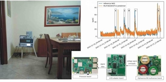
The signal chain conversion. Sensors are mounted on the Alphasense B4 multisensor board which converts sensor electric currents featured by sensitivity, shown in Table 2, into voltage levels, characterized by a sensitivity expressed in mV/ppb. Finally, the LCSS adapter board converts analog voltage signals into digital data and transmits them through a USB connection to the processor board, where they are processed by the calibration algorithms.
Figure 2.
The signal chain conversion. Sensors are mounted on the Alphasense B4 multisensor board which converts sensor electric currents featured by sensitivity, shown in Table 2, into voltage levels, characterized by a sensitivity expressed in mV/ppb. Finally, the LCSS adapter board converts analog voltage signals into digital data and transmits them through a USB connection to the processor board, where they are processed by the calibration algorithms.

Figure 3.
The experimental setup (a) and its location in the apartment (b). The size of the apartment’s daytime area is about 54 square meters.
Figure 3.
The experimental setup (a) and its location in the apartment (b). The size of the apartment’s daytime area is about 54 square meters.

Figure 4.
Domestic pollutants statistics. NO2, O3, and CO concentrations have been measured using the reference instruments (a). Temperature and relative humidity data given by the sensors inside the AQM (b).
Figure 4.
Domestic pollutants statistics. NO2, O3, and CO concentrations have been measured using the reference instruments (a). Temperature and relative humidity data given by the sensors inside the AQM (b).

Figure 5.
Time series related to the calibration period: (a) COB4(2) sensor calibrated by ANN and predictor set CO(2), (b) NOB43F(1) sensor calibrated by MLR and predictor set NO2(1), (c) OXB431(1) sensor calibrated by MLR and predictor set O3(1). Events occurring during the experiment are marked as follows. A: food cooking using natural gas burners, B: tobacco smoke, C: candles burning, D: tobacco smoke and laser printer use, E: tobacco smoke and candles burning, F: tobacco smoke and food cooking using natural gas burner, G: food cooking using natural gas burners.

Figure 6.
Time series related to the validation period: (a) COB4(2) sensor calibrated by ANN and predictor set CO(2), (b) NOB43F(1) sensor calibrated by MLR and predictor set NO2(1), (c) OXB431(1) sensor calibrated by MLR and predictor set O3(1). Events occurring during the experiment are marked as follows. A: food cooking using natural gas burners, B: tobacco smoke, C: candles burning, D: tobacco smoke and laser printer use, E: tobacco smoke and food cooking using natural gas burners, F: food cooking using natural gas burner, G: candles burning and tobacco smoke.

Figure 7.
Scatter plots for CO concentration predictions related to (a) calibration dataset, (b) validation dataset.
Figure 7.
Scatter plots for CO concentration predictions related to (a) calibration dataset, (b) validation dataset.

Figure 8.
Scatter plots for NO2 concentration predictions related to (a) calibration dataset, (b) validation dataset.
Figure 8.
Scatter plots for NO2 concentration predictions related to (a) calibration dataset, (b) validation dataset.

Figure 9.
Scatter plots for O3 concentration predictions related to (a) calibration dataset, (b) validation dataset.
Figure 9.
Scatter plots for O3 concentration predictions related to (a) calibration dataset, (b) validation dataset.

Figure 10.
Performance analysis by different predictor subsets related to the (a) calibration dataset, (b) validation dataset.
Figure 10.
Performance analysis by different predictor subsets related to the (a) calibration dataset, (b) validation dataset.


Table 1.
A summary of results concerning previous studies in terms of squared correlation coefficient (R2). This table aims to provide an indicative summary of the performance achievable through the different calibration techniques in the outdoor environment. Data are for minimum and maximum values.
| Reference | Calibration Algorithm | Target Gases | R2 |
|---|---|---|---|
| Castell [4] | LR | CO, NO2, NO, O3 | 0.008 (O3)–0.96 (NO) |
| Zimmermann [12] | RF | CO, O3, NO2 | 0.75 (NO2)–0.92 (O3) |
| Cordero [13] | MLR, RF, SVM, ANN | NO2 | 0.62 (ANN)–0.95 (RF) |
| Bigi [14] | MLR, RF, SVM | NO, NO2 | 0.6 (NO2, MLR)–0.96 (NO, SVM) |
| Suriano [15] | MLR, LR | NO2, O3 | 0.36 (NO2, LR)–0.67 (NO2, MLR) |
| Spinelle [16,17] | LR, MLR, ANN | NO2, O3, NO | 0.004 (NO2, LR)–0.915 (O3, ANN) |
| Wei [18] | MLR | CO, NO2, NO, O3 | 0.7 (O3)–0.98 (CO) |
Table 2.
The sensors used in SentinAir AQM during the experiment. The data shown in the table are reported by the manufacturer datasheets.
Table 2.
The sensors used in SentinAir AQM during the experiment. The data shown in the table are reported by the manufacturer datasheets.
| Sensor | Measured Parameter | Range | Sensitivity | Manufacturer |
|---|---|---|---|---|
| COB4 | CO | 0/1000 ppm | 350/500nA/ppm | Alphasense [31] |
| NO2B43F | NO2 | 0/20 ppm | −200/−650nA/ppm | Alphasense |
| OXB431 | O3 | 0/20 ppm | −225/−750 nA/ppm | Alphasense |
| HIH5031 | Relative humidity | 0/100% | 20 mV/RH% | Honeywell [32] |
| TC1047A | Temperature | −40 °C/+85 °C | 10 mV/°C | Microchip [33] |
Table 3.
The sensitivity values set at the sensor board output. Two sets of sensors composed of the same sensor type were involved in the experiment.
Table 3.
The sensitivity values set at the sensor board output. Two sets of sensors composed of the same sensor type were involved in the experiment.
| Sensor | Sensitivity |
|---|---|
| COB4(1) | 620 mV/ppm |
| NO2B43F(1) | 1.1 mV/ppb |
| OXB431(1) | 1.1 mV/ppb |
| COB4(2) | 580 mV/ppm |
| NO2B43F(2) | 1 mV/ppb |
| OXB431(2) | 1 mV/ppb |
Table 4.
The sets of predictors selected for each pollutant. The subscripts “w” and “a” indicate the “working” and the “auxiliary” signal electrodes, respectively. T and RH are the temperature and the relative humidity measurements carried out by the dedicated sensors. In parentheses is indicated the group of sensors.
| Calibration Model | Pollutant | Predictor Set Name | Predictor Variables |
|---|---|---|---|
| MLR, RF, SVM, ANN | CO | CO(1) | COB4(1)w, COB4(1)a, T, RH |
| CO(1)net | (COB4(1)w – COB4(1)a), T, RH | ||
| CO(2) | COB4(2)w, COB4(2)a, T, RH | ||
| CO(2)net | (COB4(2)w – COB4(2)a), T, RH | ||
| NO2 | NO2(1) | NO2B43F(1)w, NO2B43F(1)a, T, RH | |
| NO2(1)net | (NO2B43F(1)w – NO2B43F(1)a), T, RH | ||
| NO2(2) | NO2B43F(2)w, NO2B43F(2)a, T, RH | ||
| NO2(2)net | (NO2B43F(2)w – NO2B43F(2)a), T, RH | ||
| O3 | O3(1) | (OXB431(1)w – NO2B43F(1)w), OXB431(1)a, NO2B43F(1)a, T, RH | |
| O3(1)net | (OXB431(1)w – OXB431(1)a) – (NO2B43F(1)w – NO2B43F(1)a), T, RH | ||
| O3(2) | (OXB431(2)w – NO2B43F(2)w), OXB431(2)a, NO2B43F(2)a, T, RH | ||
| O3(2)net | (OXB431(2)w – OXB431(2)a) – (NO2B43F(2)w – NO2B43F(2)a), T, RH |
Table 5.
Synoptic view of results. Bold fonts show the best values for each indicator by considering calibration or validation datasets. MAE and RMSE related to NO2B43F and OXB431 are expressed as “ppb”, while those referring to COB4 are shown as “ppm”. Data highlighted in light blue are related to Figure 5, Figure 6, Figure 7, Figure 8 and Figure 9.
| Calibration | Validation | |||||||
|---|---|---|---|---|---|---|---|---|
| Gas | Model | Predictors | R2 | MAE | RMSE | R2 | MAE | RMSE |
| CO | MLR | CO(1) | 0.974 | 0.084 | 0.126 | 0.891 | 0.121 | 0.164 |
| CO(1)net | 0.961 | 0.119 | 0.155 | 0.756 | 0.213 | 0.245 | ||
| CO(2) | 0.975 | 0.083 | 0.123 | 0.918 | 0.099 | 0.140 | ||
| CO(2)net | 0.962 | 0.116 | 0.152 | 0.789 | 0.191 | 0.227 | ||
| RF | CO(1) | 0.996 | 0.017 | 0.049 | 0.912 | 0.141 | 0.149 | |
| CO(1)net | 0.996 | 0.019 | 0.052 | 0.891 | 0.173 | 0.162 | ||
| CO(2) | 0.997 | 0.016 | 0.044 | 0.897 | 0.180 | 0.156 | ||
| CO(2)net | 0.966 | 0.019 | 0.049 | 0.868 | 0.205 | 0.177 | ||
| SVM | CO(1) | 0.981 | 0.076 | 0.108 | 0.844 | 0.138 | 0.193 | |
| CO(1)net | 0.971 | 0.104 | 0.134 | 0.461 | 0.393 | 0.485 | ||
| CO(2) | 0.980 | 0.080 | 0.110 | 0.740 | 0.211 | 0.251 | ||
| CO(2)net | 0.971 | 0.100 | 0.132 | 0.420 | 0.401 | 0.489 | ||
| ANN | CO(1) | 0.975 | 0.090 | 0.124 | 0.914 | 0.403 | 0.385 | |
| CO(1)net | 0.971 | 0.098 | 0.132 | 0.906 | 0.409 | 0.351 | ||
| CO(2) | 0.975 | 0.083 | 0.124 | 0.924 | 0.377 | 0.366 | ||
| CO(2)net | 0.973 | 0.093 | 0.127 | 0.900 | 0.431 | 0.363 | ||
| NO2 | MLR | NO2(1) | 0.641 | 4.244 | 6.148 | 0.890 | 8.381 | 10.618 |
| NO2(1)net | 0.633 | 4.265 | 6.152 | 0.866 | 8.494 | 10.673 | ||
| NO2(2) | 0.598 | 4.560 | 6.433 | 0.809 | 11.923 | 12.902 | ||
| NO2(2)net | 0.560 | 4.797 | 6.738 | 0.776 | 10.413 | 13.627 | ||
| RF | NO2(1) | 0.906 | 2.011 | 3.166 | 0.600 | 9.647 | 16.305 | |
| NO2(1)net | 0.905 | 2.014 | 3.169 | 0.601 | 9.643 | 16.304 | ||
| NO2(2) | 0.912 | 1.948 | 3.052 | 0.697 | 8.656 | 14.749 | ||
| NO2(2)net | 0.890 | 2.154 | 3.401 | 0.690 | 9.361 | 15.260 | ||
| SVM | NO2(1) | 0.341 | 4.982 | 8.677 | 0.039 | 21.921 | 24.556 | |
| NO2(1)net | 0.241 | 4.981 | 8.676 | 0.039 | 21.917 | 24.553 | ||
| NO2(2) | 0.239 | 4.990 | 8.696 | 0.037 | 21.869 | 24.593 | ||
| NO2(2)net | 0.233 | 5.008 | 8.728 | 0.035 | 21.810 | 24.657 | ||
| ANN | NO2(1) | 0.776 | 3.289 | 4.861 | 0.774 | 9.551 | 15.143 | |
| NO2(1)net | 0.778 | 3.277 | 4.832 | 0.783 | 9.312 | 14.910 | ||
| NO2(2) | 0.820 | 2.912 | 4.339 | 0.478 | 10.094 | 17.949 | ||
| NO2(2)net | 0.757 | 3.460 | 5.064 | 0.809 | 10.225 | 15.439 | ||
| O3 | MLR | O3(1) | 0.432 | 6.318 | 9.401 | 0.137 | 9.552 | 16.340 |
| O3(1)net | 0.465 | 6.180 | 9.117 | 0.124 | 14.785 | 16.067 | ||
| O3(2) | 0.474 | 6.167 | 9.035 | 0.098 | 18.364 | 16.195 | ||
| O3(2)net | 0.455 | 6.124 | 9.201 | 0.108 | 15.193 | 15.892 | ||
| RF | O3(1) | 0.850 | 3.151 | 4.905 | 0.074 | 12.160 | 17.981 | |
| O3(1)net | 0.925 | 1.918 | 3.412 | 0.024 | 14.006 | 18.474 | ||
| O3(2) | 0.929 | 1.845 | 3.340 | 0.023 | 15.913 | 19.609 | ||
| O3(2)net | 0.917 | 2.044 | 3.605 | 0.026 | 13.368 | 17.880 | ||
| SVM | O3(1) | 0.379 | 6.658 | 11.796 | 0.101 | 8.533 | 11.513 | |
| O3(1)net | 0.247 | 6.287 | 10.463 | 0.008 | 17.980 | 14.826 | ||
| O3(2) | 0.260 | 6.256 | 10.380 | 0.008 | 18.628 | 15.052 | ||
| O3(2)net | 0.257 | 6.269 | 10.402 | 0.008 | 16.600 | 15.101 | ||
| ANN | O3(1) | 0.860 | 3.206 | 4.668 | 0.006 | 11.060 | 17.449 | |
| O3(1)net | 0.883 | 2.950 | 4.287 | 0.001 | 11.989 | 17.869 | ||
| O3(2) | 0.862 | 3.190 | 4.630 | 0.006 | 11.258 | 17.726 | ||
| O3(2)net | 0.763 | 4.567 | 6.075 | 0.001 | 12.683 | 21.823 | ||
Table 6.
Median values obtained from calibration dataset. Bold characters indicate the best value for each column.
Table 6.
Median values obtained from calibration dataset. Bold characters indicate the best value for each column.
| CO | NO2 | O3 | ||||
|---|---|---|---|---|---|---|
| Model | R2 | nRMSE | R2 | nRMSE | R2 | nRMSE |
| MLR | 0.968 | 0.207 | 0.615 | 0.588 | 0.460 | 1.855 |
| RF | 0.966 | 0.047 | 0.906 | 0.296 | 0.921 | 0.355 |
| SVM | 0.975 | 0.248 | 0.240 | 0.812 | 0.258 | 0.636 |
| ANN | 0.974 | 0.128 | 0.777 | 0.453 | 0.861 | 0.323 |
Table 7.
Median values obtained from validation dataset. Bold characters indicate the best value for each column.
Table 7.
Median values obtained from validation dataset. Bold characters indicate the best value for each column.
| CO | NO2 | O3 | ||||
|---|---|---|---|---|---|---|
| Model | R2 | nRMSE | R2 | nRMSE | R2 | nRMSE |
| MLR | 0.840 | 0.319 | 0.837 | 0.586 | 0.116 | 1.237 |
| RF | 0.894 | 0.259 | 0.649 | 0.784 | 0.025 | 1.399 |
| SVM | 0.600 | 0.600 | 0.038 | 1.221 | 0.008 | 1.147 |
| ANN | 0.910 | 0.594 | 0.778 | 0.760 | 0.004 | 1.366 |
Table 8.
Comparison between this work and data reported in Tryner’s study. In this table, the median values are shown for each indicator, while data in parentheses are relative to the validation period; “n.a.” stands for not applicable. MAE and RMSE for CO are expressed as “ppm”, while in the other cases, they are shown as “ppb”.
| Tryner [25] | This Work | |||||
|---|---|---|---|---|---|---|
| Pollutant | R2 | MAE | RMSE | R2 | MAE | RMSE |
| CO | 0.846 (n.a.) | 0.499 (n.a.) | 0.650 (n.a.) | 0.970 (0.867) | 0.083 (0.208) | 0.124 (0.236) |
| NO2 | 0.902 (n.a.) | 14 (n.a.) | 19 (n.a.) | 0.696 (0.713) | 3.852 (9.870) | 5.606 (15.349) |
| O3 | 0.313 (n.a.) | 15 (n.a.) | 21 (n.a.) | 0.660 (0.017) | 5.345 (13.687) | 7.555 (16.894) |
Table 9.
Comparison with previous works performed in an outdoor environment related to the R2 indicator.
Table 9.
Comparison with previous works performed in an outdoor environment related to the R2 indicator.
| Previous Works [5] | This Study | ||||
| Pollutant | Model | Calibration | Validation | Calibration | Validation |
| CO | ANN | - | 0.58 | 0.974 | 0.910 |
| CO | MLR | 0.89 | 0.83 | 0.968 | 0.840 |
| CO | RF | 0.91 | - | 0.966 | 0.894 |
| NO2 | ANN | 0.87 | 0.94 | 0.777 | 0.778 |
| NO2 | MLR | 0.81 | 0.81 | 0.615 | 0.840 |
| NO2 | SVM | - | 0.78 | 0.240 | 0.038 |
| O3 | ANN | - | 0.89 | 0.861 | 0.004 |
| O3 | MLR | 0.91 | 0.88 | 0.460 | 0.116 |
Publisher’s Note: MDPI stays neutral with regard to jurisdictional claims in published maps and institutional affiliations. |
© 2022 by the authors. Licensee MDPI, Basel, Switzerland. This article is an open access article distributed under the terms and conditions of the Creative Commons Attribution (CC BY) license (https://creativecommons.org/licenses/by/4.0/).
Share and Cite
MDPI and ACS Style
Suriano, D.; Penza, M. Assessment of the Performance of a Low-Cost Air Quality Monitor in an Indoor Environment through Different Calibration Models. Atmosphere 2022, 13, 567. https://0-doi-org.brum.beds.ac.uk/10.3390/atmos13040567
AMA Style
Suriano D, Penza M. Assessment of the Performance of a Low-Cost Air Quality Monitor in an Indoor Environment through Different Calibration Models. Atmosphere. 2022; 13(4):567. https://0-doi-org.brum.beds.ac.uk/10.3390/atmos13040567
Chicago/Turabian StyleSuriano, Domenico, and Michele Penza. 2022. "Assessment of the Performance of a Low-Cost Air Quality Monitor in an Indoor Environment through Different Calibration Models" Atmosphere 13, no. 4: 567. https://0-doi-org.brum.beds.ac.uk/10.3390/atmos13040567
Note that from the first issue of 2016, this journal uses article numbers instead of page numbers. See further details here.