
Interfacial Properties of H2O+CO2+Oil Three-Phase Systems: A Density Gradient Theory Study


1
State Key Laboratory for Geomechanics and Deep Underground Engineering, China University of Mining and Technology, Xuzhou 221116, China
2
School of Mechanics and Civil Engineering, China University of Mining and Technology, Xuzhou 221116, China
3
Department of Engineering Mechanics, Tsinghua University, Beijing 100084, China
4
State Key Laboratory of Coal Mining and Clean Utilization, China Coal Research Institute, Beijing 100013, China
*
Authors to whom correspondence should be addressed.
Atmosphere 2022, 13(4), 625; https://0-doi-org.brum.beds.ac.uk/10.3390/atmos13040625
Submission received: 25 March 2022
/
Revised: 8 April 2022
/
Accepted: 12 April 2022
/
Published: 14 April 2022
(This article belongs to the Special Issue Recent Advances in Gases Adsorption and Transport Behavior)
Abstract
:The interfacial property of HO+CO+oil three-phase systems is crucial for CO flooding and sequestration processes but was not well understood. Density gradient theory coupled with PC-SAFT equation of state was applied to investigate the interfacial tension (IFT) of HO+CO+oil (hexane, cyclohexane, and benzene) systems under three-phase conditions (temperature in the range of 323–423 K and pressure in the range of 1–10 MPa). The IFTs of the aqueous phase+vapor phase in HO+CO+oil three-phase systems were smaller than the IFTs in HO+CO two-phase systems, which could be explained by enrichment of oil in the interfacial region. The difference between IFTs of aqueous phase+vapor phase in the three-phase system and IFTs in HO+CO two-phase system was largest in the benzene case and smallest in the cyclohexane case due to different degrees of oil enrichment in the interface. Meanwhile, CO enrichment was observed in the interfacial region of the aqueous phase+oil-rich phase, which led to the reduction of IFT with increasing pressure while different pressure effects were observed in the HO+oil two-phase systems. The effect of CO on the IFTs of aqueous phase+benzene-rich phase interface was small in contrast to that on the IFTs of aqueous phase+alkane (hexane or cyclohexane)-rich phase interface. HO had little effect on the interfacial properties of the oil-rich phase+vapor phase due to the low HO solubilities in the oil and vapor phase. Further, the spreading coefficients of HO+CO in the presence of different oil followed this sequence: benzene > hexane > cyclohexane.
1. Introduction
Recently, many countries around the world have targeted net-zero carbon emissions in the following few decades to mitigate global warming [1,2,3]. CO flooding techniques have demonstrated great potential in offsetting greenhouse emissions and increasing oil recovery efficiency at the same time [4,5,6]. Although CO miscible flooding is one of the most effective methods of enhancing oil recovery, a significant amount of reservoir conditions cannot meet the miscible requirements because of either technical issues or economic considerations [7]. Hence CO near-miscible or immiscible flooding may be applied when the pressure condition does not allow CO to fully dissolve in oil [8]. During near-miscible or immiscible water alternating gas injection processes, interfacial tension (IFT) of HO+CO+oil three-phase systems is of great importance since it can determine the capillary force that displaces oil and stores CO in geological formations [4,9].
There has been a considerable number of studies on the interfacial properties of two-phase systems containing HO, CO and/or oil [10,11,12,13,14,15,16,17,18,19,20,21,22]. Generally, the IFT of HO+CO two-phase system decreases with increasing temperature and pressure [10,16,20]. However, at relatively high pressures, the IFT increases with increasing pressure [17]. The IFT of HO+oil two-phase systems usually increases with decreasing temperature and increasing pressure [11,23,24,25]. When HO+oil two-phase systems are in contact with CO under miscible conditions, the IFT increases with decreasing CO mole fraction mainly because of the positive surface excess of CO in the interface [19,21,24]. The IFT in the oil+CO two-phase system decreases with pressure and at elevated temperatures, the reduction of IFT due to pressure increment decreases [18,26,27]. Although a few studies on the interfacial properties of water+gas+oil three-phase systems have been carried out [28,29,30,31,32], interfacial properties of HO+CO+oil three-phase system have not been investigated yet.
In this work, we studied the interfacial properties of HO+CO+oil three-phase systems at different temperatures (323, 373, and 423 K) and pressures (1–10 MPa). The temperature and pressure conditions chosen here are typical reservoir conditions during CO near-miscible or immiscible flooding [33,34]. The composition of crude oil is complex, and the predominant components are aliphatic, alicyclic and aromatic hydrocarbons [35,36,37]. Hence, hexane, cyclohexane, and benzene were selected to represent these hydrocarbon types in this study. The IFTs were calculated by density gradient theory (DGT) coupled with the perturbed-chain statistical associating fluid theory (PC-SAFT) equation of state (EoS). The component density distributions and surface excess in the interfacial region were analyzed to understand the behavior of IFT of three-phase systems at geological conditions.
2. Theoretical Details
PC-SAFT EoS was applied to estimate the bulk properties of fluid mixtures. The EoS can be expressed via the compressibility factor Z [38,39]:
where is the hard-chain term, is the dispersive part, and represents the contribution due to association. Z is a function of the segment number , the segment diameter , and the segment energy parameter . HO was modeled with 4C association scheme, and CO and benzene can cross-associate with HO [40]. The parameters for a pair of unlike segments were estimated using the Lorentz-Berthelot combining rules [38]:
where is the binary interaction parameter. The EoS parameters are given in Table 1 and Table 2. Most of the parameters were taken from previous studies [21,22,24,38,41,42]. The missing parameter was fitted based on experimental data [43].
PC-SAFT EoS was coupled with the DGT for the estimation of interfacial properties. Briefly, for a planar interface of area A, the Helmholtz free energy is given as [44,45]:
where denotes the Helmholtz free energy density of the homogeneous fluid at the local density n, represents the local density gradient of the ith component. The cross influence parameter is defined as [46,47,48]:
where and represent the pure component influence parameters, and denote the binary interaction coefficient. These parameters were given in Table 3 and Table 4, and they were fitted in previous studies of two-phase systems [21,22,42,49].
In equilibrium, the density profiles across the interface were evaluated through the minimization of the free energy by solving the corresponding Euler-Lagrange equation [44,45]:
where is the chemical potential of the ith component in the bulk phase (), represents the chemical potential of the ith component and denotes the total number of components. These equations were solved together with the boundary conditions obtained from three-phase flash calculations [50]:
where and represent the bulk densities of the coexisting phases and l denotes the interfacial thickness of one interface in three-phase system. When the equilibrium density profiles were available, the interfacial tension () was estimated as follows [44,45]:
Figure 1a displays the schematic illustration of HO+CO+oil three-phase system. The DGT was applied for each pair of phases in the three-phase systems for calculating the interfacial properties [51]. Once the IFTs of each interface were obtained, the spreading coefficient S can be estimated as [52]:
where is the IFT of the aqueous phase+vapor phase, is the IFT of the oil-rich phase+aqueous phase, and is the IFT of the oil-rich phase+vapor phase in the three-phase system. The spreading coefficient can be used to gauge the capability of oil to form a spreading film between HO and vapor [52,53]. Figure 1b shows the schematic illustration of oil spreading between HO and vapor. If S is positive, the oil film will form separating the aqueous phase and vapor phase, and a negative S indicates the formation of an oil lens [54,55].
3. Results and Discussion
3.1. Model Validation
To validate the models used in this study, the densities of pure component and solubilities in HO+CO, HO+oil, and oil+CO two-phase systems were predicted by PC-SAFT EoS and compared with experimental data [43,56,57,58,59,60,61] in Figures S1–S6. We also calculated the IFT of HO+CO, HO+oil, and oil+CO two-phase systems and compared the IFTs with experimental data [10,11,12,13,14,15] as shown in Figures S7–S9. Good agreement was obtained between theory and experiment. For example, the maximum IFT deviation is around 4 mN/m. Figures S10–S19 show the calculated density distributions and component surface excess [16,18,62] in the two-phase systems. Although it is challenging to measure the component distributions in the interfacial region in experiment [63], the calculated interfacial properties were in reasonable agreement with previous simulation and theoretical studies of two-phase systems [16,18,20,21,22].
3.2. Interfacial Properties of HO+CO+Hexane Three-Phase System
3.2.1. Interface of Aqueous Phase+Vapor Phase
Figure 2a presents the IFT obtained from DGT for the interface of aqueous phase+vapor phase in HO+CO+hexane three-phase system. The IFT falls in the range of 31.4 to 55.0 mN/m at studied conditions. The IFT decreases with pressure and temperature, which is similar to previous studies on the HO+CO two-phase system [10,16,20,64]. The three-phase IFTs were plotted together with two-phase IFTs shown as dashed lines (also see Figure S7). It can be observed that the IFTs are significantly smaller in three-phase cases than those in two-phase cases. For instance, the difference between those two IFT values falls in the range of 2.7–6.3 mN/m. Furthermore, the reduction of IFT is larger at high temperatures and low pressures.
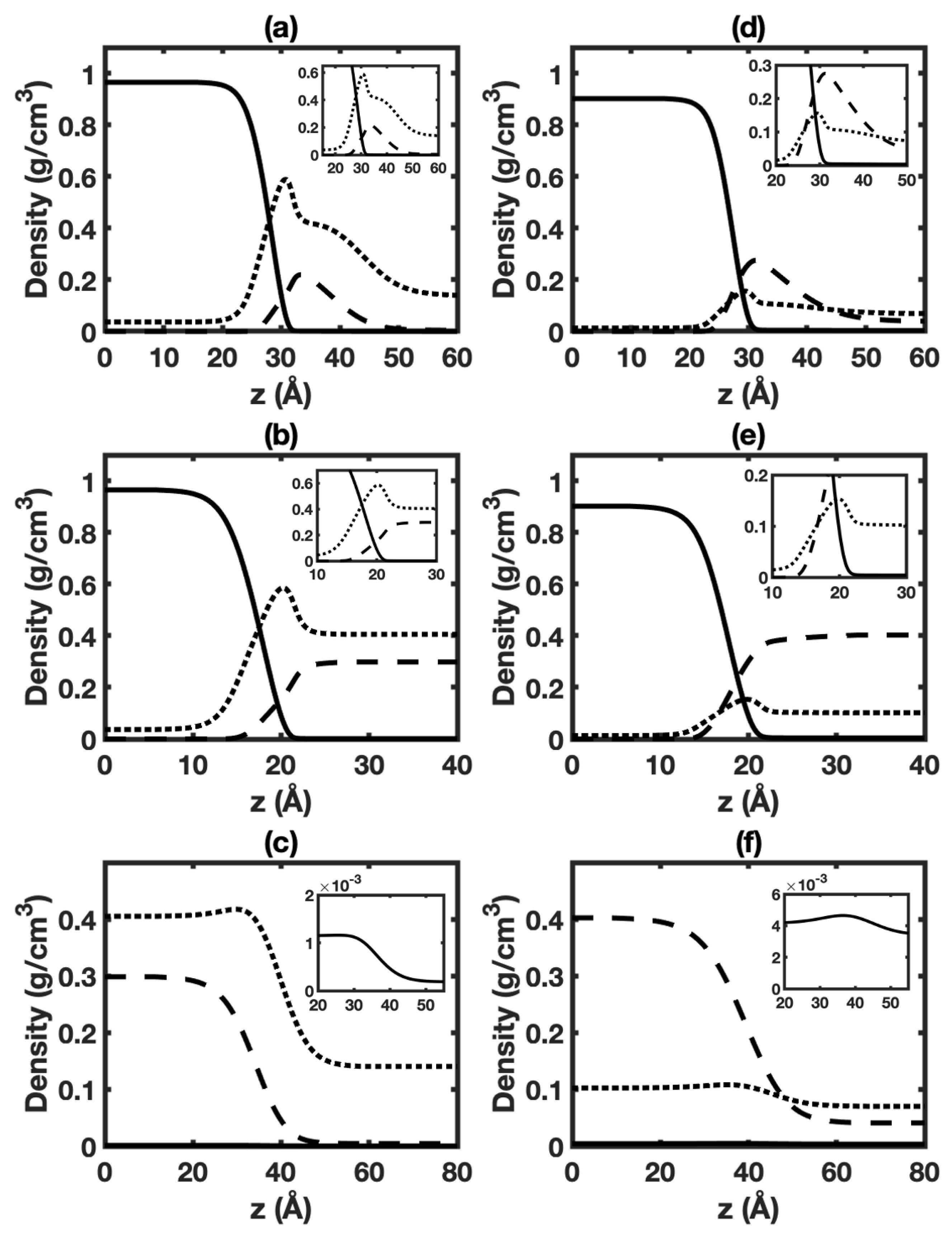
Figure 3a,d display density distributions of HO, CO, and hexane as calculated by DGT in the interfacial region between the aqueous phase and vapor phase in the three-phase system at 6 MPa and different temperatures. Corresponding cases at 1 MPa are given in Figure S20a,d. The shapes of HO and CO density profiles are similar to those of the HO+CO two-phase system [16,20,64] (also see Figure S10). The density profile of HO is close to a hyperbolic tangent function. Enrichment of CO in the interfacial region can be observed in all cases. Remarkably, enrichment of hexane in the interfacial region is also seen. The enrichment of hexane is likely due to the hydrophobic interaction between HO and oil.
Surface excess can gauge the component enrichment in the interfacial region [16,18,62]. The behavior of IFT is associated with surface excess through the Gibbs adsorption equation [24,62]. Figure S21a,d show the surface excess of CO and hexane (HO is selected as the reference). The surface excess of CO is consistent with that of the HO+CO two-phase system in the previous study [62] (also see Figure S17). The CO surface excess decreases with increasing temperature, and it increases with increasing pressure. The hexane surface excesses are all positive, which gives rise to the reduction of IFT when hexane is included in the system based on the Gibbs adsorption equation. Hexane surface excess is enhanced by high pressure, possibly because of the relatively higher oil solubility in the vapor phase at high pressure [27]. High temperature increases the hexane surface excess due to the increase of oil solubility in vapor at high temperatures.
3.2.2. Interface of Aqueous Phase+Hexane-Rich Phase
Figure 2b presents the IFTs for the interface of aqueous phase+hexane-rich phase in HO+CO+hexane three-phase system. The IFT decreases with increasing pressure and temperature, and falls in the range of 30.4 to 44.9 mN/m. As temperature increases, the reduction of IFT due to pressure increment decreases. For example, at 373 K, the IFT decreases by about 10.7 mN/m from 42.6 to 31.9 mN/m when increasing pressure from 1 to 10 MPa. While at 423 K, the IFT decreases by around 6.5 nN/m from 36.9 to 30.4 mN/m with the same pressure increase. The three-phase IFT data were plotted together with HO+hexane two-phase IFT data as dashed lines (also see Figure S8a). The IFT in HO+hexane two-phase system without CO behaves significantly different from those in the three-phase system. The IFT of HO+hexane two-phase system increases with increasing pressure and is larger than that in the three-phase system, especially at low temperature and high pressure conditions. For example, at 323 K and 8 MPa, the IFT difference can be up to 18.1 mN/m.
Figure 3b,e display density profiles of HO, CO, and hexane for the interface of aqueous phase+oil-rich phase in the three-phase system at 6 MPa and different temperatures. Corresponding cases at 1 MPa are given in Figure S20b,e. The shape of HO and hexane density profiles is similar to that of the HO+hexane two-phase system [21] (also see Figure S14). The density profiles of HO and hexane can be approximated by a hyperbolic tangent function. Importantly, enrichment of CO in the interface is observed in all cases.
Figure S21b,e show the calculated surface excess of CO and hexane with HO as the reference component. The surface excess of hexane is mostly negative and generally increases with temperature. However, in HO-hexane two-phase system, an opposite temperature effect was reported [21] (also see Figure S18a). Meanwhile, the CO surface excess is positive and increases with pressure and decreases with temperature. Based on the Gibbs adsorption equation, the effect of pressure on IFT in the three-phase system could be mainly explained by the positive CO surface excess.
3.2.3. Interface of Hexane-Rich Phase+Vapor Phase
Figure 2c gives the IFTs for the interface of hexane-rich phase+vapor phase in HO+CO+ hexane three-phase system. The IFTs are almost the same as those in the hexane+CO two-phase system (also see Figure S9a). The negligible effect of HO on IFT is likely due to minor HO solubility in the oil-rich [24] and vapor [20] phase. Figure 3c,f and Figure S20c,f present the density profiles. Only a slight difference can be observed when comparing them with density profiles in the hexane+CO two-phase system shown in Figure S14. The difference between CO surface excess with hexane as the reference component in the three-phase system (see Figure S21c) and that in the two-phase system (see Figure S19a) is small. Remarkably, positive HO surface excesses are predicted. As shown in Figure S21f, HO surface excesses increase with temperature and generally increase as pressure increases. The positive HO surface excesses indicate HO enrichment in the interfacial region.
3.3. Interfacial Properties of HO+CO+Cyclohexane Three-Phase System
3.3.1. Interface of Aqueous Phase+Vapor Phase
Figure 4a presents the IFTs for the interface of aqueous phase+vapor phase in HO+CO+ cyclohexane three-phase system. The IFTs decrease with pressure and temperature, similar to the HO+CO+hexane three-phase system mentioned above. The IFTs fall in the range of 31.7 to 57.1 mN/m, which are slighter higher than the IFTs in HO+CO+hexane three-phase system indicating the smaller effect of cyclohexane on IFT than that of hexane. The three-phase IFT data were plotted together with two-phase IFT data as dashed lines, and the difference between three-phase and two-phase IFT falls in the range of 2.4–6.3 mN/m.
Figure 5a,d display density profiles of HO, CO, and cyclohexane for the interface of aqueous phase+vapor phase in the three-phase system at 6 MPa and different temperatures. Corresponding cases at 1 MPa are given in Figure S22a,d. The shape of density profiles is similar to that in HO+CO+hexane three-phase system. The enrichment of cyclohexane in the interfacial region is observed. But the enrichment of cyclohexane is smaller than that of hexane. This is likely due to the larger size of the cyclohexane molecule, which leads to smaller cyclohexane solubility in bulk phases.
Figure S23a,d give the calculated surface excesses of CO and cyclohexane (HO is chosen as the reference component). The cyclohexane surface excess is found to be positive over the studied conditions, which leads to the reduction of IFT in the presence of hexane. Remarkably, the surface excess of cyclohexane is generally smaller than that of hexane discussed in the above section, which could explain its relatively smaller effect on IFT.
3.3.2. Interface of Aqueous Phase+Cyclohexane-Rich Phase
Figure 4b presents the IFT for the interface of aqueous phase+cyclohexane-rich phase in HO+CO+cyclohexane three-phase system. The IFTs decrease with increasing pressure and temperature, and fall in the range of 30.3 to 46.7 mN/m. As temperature increases, the reduction of IFT due to pressure increment decreases. The three-phase IFT data were plotted together with HO+cyclohexane two-phase IFT data as dashed lines (also see Figure S8b). Similar to the hexane case, the IFTs without CO are significantly different from those in the three-phase system. The IFTs of HO+cyclohexane two-phase system increase with increasing pressure and are larger than those in the three-phase system, especially at low temperature and high pressure conditions.
Figure 5b,e display density profiles of HO, CO, and cyclohexane for the interface of aqueous phase+cyclohexane-rich phase in the three-phase system at 6 MPa and different temperatures. Corresponding cases at 1 MPa are given in Figure S22b,e. The shape of HO and cyclohexane density profiles is similar to that of the HO+cyclohexane two-phase system [21] (also see Figure S12). The density profiles of HO and cyclohexane can also be approximated by a hyperbolic tangent function. Enrichment of CO is seen in all cases.
Figure S23b,e show the calculated surface excess of CO and cyclohexane with HO as the reference component. The surface excess of cyclohexane is negative and increases with temperature. However, in HO-cyclohexane two-phase system, an opposite temperature effect was reported [21] (also see Figure S18b). Meanwhile, the CO surface excess is positive and generally increases with pressure and decreases with temperature. Based on the Gibbs adsorption equation, the effect of pressure on IFT in the three-phase system can be mainly explained by the positive CO surface excess.
3.3.3. Interface of Cyclohexane-Rich Phase+Vapor Phase
Figure 4c displays the IFTs for the interface of cyclohexane-rich phase+vapor phase in HO+CO+cyclohexane three-phase system. Similar to the corresponding case with hexane, the IFTs are almost the same as those in the cyclohexane+CO two-phase system (also see Figure S9b). Figure 5c,f and Figure S22c,f present the corresponding density profiles. Only very little difference can be seen comparing them with density profiles in the cyclohexane+CO two-phase system shown in Figure S15. As expected, the difference between CO surface excess in the three-phase system (Figure S23c) and that in the two-phase system (Figure S19b) is minor. As shown in Figure S23f, HO surface excess is positive, and the HO surface excess increases with temperature and pressure.
3.4. Interfacial Properties of HO+CO+Benzene Three-Phase System
3.4.1. Interface of Aqueous Phase+Vapor Phase
Figure 6a presents the IFTs for the interface of aqueous phase+vapor phase in HO+CO+ benzene three-phase system. The IFTs decrease with pressure and temperature, similar to the HO+CO+alkane (hexane or cyclohexane) three-phase systems mentioned above. The IFTs fall in the range of 21.6 to 47.4 mN/m, which are much lower than the IFTs in HO+CO+alkane three-phase systems. This indicates the strong effect of benzene on IFT than that of alkane possibly due to the strong association between benzene and HO. The three-phase IFT data were plotted together with two-phase IFT data in dashed lines. The difference between three-phase and two-phase IFT decreases as pressure increases and temperature decreases, and falls in the range of 8.1–15.5 mN/m.
Figure 7a,d displays the density profiles of HO, CO, and benzene for the interface of aqueous phase+vapor phase in the three-phase system at 6 MPa and different temperatures. Corresponding cases at 1 MPa are given in Figure S24a,d. The shape of density profiles is similar to that in HO+CO+alkane three-phase system. The enrichment of benzene in the interfacial region is observed. The enrichment of benzene is much stronger than those of alkanes, which can be explained by the strong hydrogen bond between HO and benzene [65].
Figure S25a,d give the calculated surface excesses of CO and benzene (HO is chosen as the reference component). The benzene surface excess is found to be positive over the studied conditions, which causes the reduction of IFT in the presence of benzene. As expected, the surface excess of benzene is larger than those of alkanes discussed in the above section, which explains its stronger effect on IFT.
3.4.2. Interface of Aqueous Phase+Benzene-Rich Phase
Figure 6b presents the IFTs for the interface of aqueous phase+benzene-rich phase in HO+CO+benzene three-phase system. The IFTs decrease with increasing pressure and temperature, and fall in the range of 18.3 to 26.1 mN/m. The three-phase IFTs were plotted together with HO+benzene two-phase IFT data as dashed lines (also see Figure S8c). The IFTs without CO behave differently from IFTs in the three-phase system. The IFTs of HO+benzene two-phase system hardly change with increasing pressure and are larger than IFTs in the three-phase system, especially at low temperature and high pressure conditions. Furthermore, the effect of CO on the IFTs of aqueous phase+benzene-rich phase interface is small compared with that on the IFTs of aqueous phase+alkane (hexane or cyclohexane)-rich phase interface.
Figure 7b,e display density profiles of HO, CO, and benzene for the interface of aqueous phase+benzene-rich phase in the three-phase system at 6 MPa and different temperatures. Corresponding cases at 1 MPa are given in Figure S24b,e. The shape of HO density profile is similar to that of the HO+benzene two-phase system [22] (also see Figure S13). Enrichment of benzene and CO are seen in the interfacial region due to relatively strong quadrupole-dipole interaction of HO-CO pair and hydrogen bonding interaction between HO and benzene.
Figure S25b,e show the calculated surface excess of CO and benzene with HO as the reference component. The surface excess of benzene is generally negative and increases with temperature. However, in HO-benzene two-phase system, an opposite temperature effect was reported [22] (also see Figure S18c). Meanwhile, the CO surface excess is positive and generally increases with pressure and decreases with temperature. Based on the Gibbs adsorption equation, the effect of pressure on IFT in the three-phase system can be mainly explained by the positive CO surface excess.
3.4.3. Interface of Benzene-Rich Phase+Vapor Phase
Figure 6c displays the IFTs for the interface of benzene-rich phase+vapor phase in HO+CO+benzene three-phase system. Similar to the corresponding cases with alkanes, the IFTs are almost the same as those in the benzene+CO two-phase system (also see Figure S9c). Figure 7c,f and Figure S24c,f present the corresponding density profiles. Only very little difference can be seen comparing them with density profiles in the benzene+CO two-phase system shown in Figure S16. As expected, the difference between CO surface excess in the three-phase system (Figure S25c) and that in the two-phase system (Figure S19c) is minor. HO surface excess is positive, and the HO surface excess increases with temperature and pressure as shown in Figure S25f.
3.5. Spreading Coefficient
Figure 8 shows the spreading coefficient of HO+CO+oil systems for different oil types at studied conditions. The spreading coefficient increases with pressure. The effect of temperature on the spreading coefficient of benzene is little, while high temperature mitigates the pressure effects on the spreading coefficient in the system with alkanes. The spreading coefficients for hexane, cyclohexane, and benzene cases fall in the range of −2.50 to 0.08, −8.63 to −0.04, and −0.05 to 0.25 mN/m, respectively. The following order is found for different oil in contact with HO+CO at the three-phase condition: benzene > hexane > cyclohexane. Based on the results in Figure 8, it can be known that the benzene film will generally form separating the aqueous and vapor phase while three-phase contact exists for hexane and cyclohexane cases under most conditions.
3.6. Bulk Properties
The effect of temperature and pressure on bulk properties depends on component and phase. Figures S26–S28 present the bulk densities in the three-phase system with different oil types. HO density in the aqueous phase decreases as pressure and temperature increase. While in the vapor and oil phase, HO density increases as pressure and temperature increase. Increasing pressure and decreasing temperature lead to an increment of CO density in all phases. Oil density decreases as pressure increases in the aqueous and oil phase, and increases as pressure increases in the vapor phase. In general, high temperature increases oil density in all phases. However, at low pressure, a reduction of oil density with increasing temperature is seen in the oil phase.
Figures S29–S31 display the solubilities in the three-phase system with different oil types. HO solubility in all phases increases with increasing temperature. HO solubility decreases as pressure increases in the aqueous and vapor phase. However, an opposite pressure effect can be seen for HO solubility in the oil phase. In all phases, CO solubility increases as temperature decreases and pressure increases. Moreover, high oil solubility was observed at low pressure and high temperature.
4. Conclusions
In this study, density gradient theory calculations coupled with PC-SAFT EoS had been carried out to study the interfacial properties in HO+CO+oil (hexane, cyclohexane, and benzene) three-phase systems at different temperatures (323, 373, and 423 K) and pressures (1–10 MPa). Generally, the IFTs in three-phase systems decreased with increasing pressure. The reduction of IFT due to pressure increment was more significant at lower temperature. Other important findings were as follows:
- The IFTs of the aqueous phase+vapor phase in HO+CO+oil three-phase systems were smaller than the IFTs in HO+CO two-phase systems, which could be explained by enrichment of oil in the interfacial region. The difference between IFTs of aqueous phase+vapor phase in the three-phase system and IFTs in HO+CO two-phase system was largest in benzene case and smallest in cyclohexane case due to different degrees of oil enrichment in the interface.
- Significant CO enrichment was observed in the interfacial region of the aqueous phase+oil-rich phase in HO+CO+oil three-phase systems. This led to the reduction of IFT with increasing pressure while different pressure effects were observed in the HO+oil two-phase systems. The effect of CO on the IFTs of aqueous phase+benzene-rich phase interface was small in contrast to that on the IFTs of aqueous phase+alkane (hexane or cyclohexane)-rich phase interface.
- The IFTs of oil-rich phase+vapor phase in HO+CO+oil three-phase systems were hardly affected by HO because of low HO solubilities in oil and vapor phases. Nevertheless, HO surface excesses were positive.
- On most conditions, benzene film formed and separated the HO phase and vapor phase while three-phase contact existed in hexane and cyclohexane cases. The spreading coefficients of HO+CO in the presence of different oil under three-phase conditions followed this sequence: benzene > hexane > cyclohexane.
This study provides a fundamental understanding of the interfacial properties of the HO+CO+oil three-phase systems. We believe it could help optimize CO near-miscible and immiscible flooding techniques.
Supplementary Materials
The following supporting information can be downloaded at: https://0-www-mdpi-com.brum.beds.ac.uk/article/10.3390/atmos13040625/s1, Figure S1: Densities of HO as a function of pressure at different temperatures. The experimental data from NIST accessed on 6 April 2022 (http://webbook.nist.gov/chemistry/fluid) are shown as solid symbols; Figure S2: Densities of CO as a function of pressure at different temperatures. The experimental data from NIST (http://webbook.nist.gov/chemistry/fluid, accessed on 6 April 2022) are shown as solid symbols; Figure S3: Densities of oil as a function of pressure at different temperatures. The experimental data from NIST (http://webbook.nist.gov/chemistry/fluid, accessed on 6 April 2022) are shown as solid symbols; Figure S4: Solubilities in HO+CO two-phase system. The experimental data is taken from (J. Supercrit. Fluids, 2013, 73: 87–96); Figure S5: Solubilities in HO+oil two-phase system. The experimental data is taken from (J. Phys. Chem. Ref. Data, 2004, 33(2): 549–577) and (J. Chem. Eng. Data, 2003, 48(3): 750–752); Figure S6: Solubilities in oil+CO two-phase system. The experimental data is taken from (Fluid Phase Equilib., 1987, 33(1-2): 109–123), (J. Chem. Eng. Data, 1987, 32(3): 369–371), and (Fluid Phase Equilib., 1987, 36: 107–119); Figure S7: Pressure dependence of IFT in water-CO two-phase system. The experimental data (J. Chem. Thermodyn., 2016, 93: 404) are shown as solid symbols; Figure S8: Pressure dependence of IFT in water+oil two-phase systems: (a) hexane; (b) cyclohexane; (c) benzene. The experimental data (J. Chem. Eng. Data, 1996, 41: 493; J. Phys. Chem., 1951, 55: 439; J. Colloid Interface Sci., 1967, 24: 323) are shown as solid symbols; Figure S9: Pressure dependence of IFT in oil+methane two-phase systems: (a) hexane; (b) cyclohexane; (c) benzene. The experimental data (Chin. J. Chem. Eng., 2014, 22: 1302; J Supercrit Fluids, 2019, 154: 104625) are shown as solid symbols; Figure S10: Equilibrium distributions of different species in water+CO two-phase system at (a) 323 K and 1 MPa, (b) 423 K and 1 MPa, (c) 323 K and 6 MPa, and (d) 423 K and 6 MPa. The solid and dashed lines denote water and CO, respectively; Figure S11: Equilibrium distributions of different species in hexane+water two-phase system at (a) 323 K and 1 MPa, (b) 423 K and 1 MPa, (c) 323 K and 6 MPa, and (d) 423 K and 6 MPa. The solid and dashed lines denote water and hexane, respectively; Figure S12: Equilibrium distributions of different species in cyclohexane+water two-phase system at (a) 323 K and 1 MPa, (b) 423 K and 1 MPa, (c) 323 K and 6 MPa, and (d) 423 K and 6 MPa. The solid and dashed lines denote water and cyclohexane, respectively; Figure S13: Equilibrium distributions of different species in benzene+water two-phase system at (a) 323 K and 1 MPa, (b) 423 K and 1 MPa, (c) 323 K and 6 MPa, and (d) 423 K and 6 MPa. The solid and dashed lines denote water and benzene, respectively; Figure S14: Equilibrium distributions of different species in hexane+CO two-phase system at (a) 323 K and 1 MPa, (b) 423 K and 1 MPa, (c) 323 K and 6 MPa, and (d) 423 K and 6 MPa. The solid and dashed lines denote hexane and CO, respectively; Figure S15: Equilibrium distributions of different species in cyclohexane+CO two-phase system at (a) 323 K and 1 MPa, (b) 423 K and 1 MPa, (c) 323 K and 6 MPa, and (d) 423 K and 6 MPa. The solid and dashed lines denote cyclohexane and CO, respectively; Figure S16: Equilibrium distributions of different species in benzene+CO two-phase system at (a) 323 K and 1 MPa, (b) 423 K and 1 MPa, (c) 323 K and 6 MPa, and (d) 423 K and 6 MPa. The solid and dashed lines denote benzene and CO, respectively; Figure S17: Pressure dependence of CO surface excess in water+CO two-phase system; Figure S18: Pressure dependence of oil surface excess in water+oil two-phase systems: (a) hexane; (b) cyclohexane; (c) benzene; Figure S19: Pressure dependence of CO surface excess in oil+CO two-phase systems: (a) hexane; (b) cyclohexane; (c) benzene; Figure S20: Same as Figure 3, but at 1 MPa; Figure S21: Pressure dependence of component surface excess in HO+CO+hexane three-phase system: (a,d) interface of aqueous phase +vapor phase (top panels); (b,e) interface of aqueous phase+hexane-rich phase (middle panels); (c,f) interface of hexane-rich phase+vapor phase (bottom panels); Figure S22: Same as Figure 5, but at 1 MPa; Figure S23: Pressure dependence of component surface excess in HO+CO+cyclohexane three-phase system: (a,d) interface of aqueous phase +vapor phase (top panels); (b,e) interface of aqueous phase+cyclohexane-rich phase (middle panels); (c,f) interface of cyclohexane-rich phase+vapor phase (bottom panels); Figure S24: Same as Figure 7, but at 1 MPa; Figure S25: Pressure dependence of component surface excess in HO+CO+benzene three-phase system: (a,d) interface of aqueous phase +vapor phase (top panels); (b,e) interface of aqueous phase+benzene-rich phase (middle panels); (c,f) interface of benzene-rich phase+vapor phase (bottom panels); Figure S26: Densities in HO+CO+hexane three-phase system. Top panels give densities in aqueous phase. Middle panels give densities in vapor phase. Bottom panels give densities in oil phase; Figure S27: Densities in HO+CO+cyclohexane three-phase system. Top panels give densities in aqueous phase. Middle panels give densities in vapor phase. Bottom panels give densities in oil phase; Figure S28: Densities in HO+CO+benzene three-phase system. Top panels give densities in aqueous phase. Middle panels give densities in vapor phase. Bottom panels give densities in oil phase; Figure S29: Solublities in HO+CO+hexane three-phase system. Top panels give solublities in aqueous phase. Middle panels give solublities in vapor phase. Bottom panels give solublities in oil phase; Figure S30: Solublities in HO+CO+cyclohexane three-phase system. Top panels give solublities in aqueous phase. Middle panels give solublities in vapor phase. Bottom panels give solublities in oil phase; Figure S31: Solublities in HO+CO+benzene three-phase system. Top panels give solublities in aqueous phase. Middle panels give solublities in vapor phase. Bottom panels give solublities in oil phase.
Author Contributions
Conceptualization, Y.Y.; methodology, Y.Y.; software, Y.Y.; validation, Y.Y.; formal analysis, Y.Y.; investigation, Y.Y.; resources, Y.Y.; data curation, Y.Y.; writing—original draft preparation, Y.Y.; writing—review and editing, Y.Y., W.Z., Y.J., T.W. and G.Z.; funding acquisition, Y.Y., T.W. and G.Z. All authors have read and agreed to the published version of the manuscript.
Funding
This research was funded by China University of Mining and Technology grant number 102521155. Supported by open fund of State Key Laboratory of Coal Mining and Clean Utilization (China Coal Research Institute) (Grant No. 2021-CMCU-KF019).
Institutional Review Board Statement
Not applicable.
Informed Consent Statement
Not applicable.
Data Availability Statement
Not applicable.
Conflicts of Interest
The authors declare no conflict of interest.
References
- Geden, O. An actionable climate target. Nat. Geosci. 2016, 9, 340–342. [Google Scholar] [CrossRef]
- Rogelj, J.; Schaeffer, M.; Meinshausen, M.; Knutti, R.; Alcamo, J.; Riahi, K.; Hare, W. Zero emission targets as long-term global goals for climate protection. Environ. Res. Lett. 2015, 10, 105007. [Google Scholar] [CrossRef]
- Rogelj, J.; Geden, O.; Cowie, A.; Reisinger, A. Three ways to improve net-zero emissions targets. Nature 2021, 591, 365–368. [Google Scholar] [CrossRef] [PubMed]
- Smit, B.; Reimer, J.A.; Oldenburg, C.M.; Bourg, I.C. Introduction to Carbon Capture and Sequestration; World Scientific: Singapore, 2014; Volume 1. [Google Scholar]
- Wei, J.; Zhou, J.; Li, J.; Zhou, X.; Dong, W.; Cheng, Z. Experimental study on oil recovery mechanism of CO2 associated enhancing oil recovery methods in low permeability reservoirs. J. Pet. Sci. Eng. 2021, 197, 108047. [Google Scholar] [CrossRef]
- Ettehadtavakkol, A.; Lake, L.W.; Bryant, S.L. CO2-EOR and storage design optimization. Int. J. Greenh. Gas Control 2014, 25, 79–92. [Google Scholar] [CrossRef]
- Zhang, N.; Wei, M.; Bai, B. Statistical and analytical review of worldwide CO2 immiscible field applications. Fuel 2018, 220, 89–100. [Google Scholar] [CrossRef]
- Gozalpour, F.; Ren, S.R.; Tohidi, B. CO2 EOR and storage in oil reservoir. Oil Gas Sci. Technol. 2005, 60, 537–546. [Google Scholar] [CrossRef] [Green Version]
- Deng, X.; Tariq, Z.; Murtaza, M.; Patil, S.; Mahmoud, M.; Kamal, M.S. Relative contribution of wettability Alteration and interfacial tension reduction in EOR: A critical review. J. Mol. Liq. 2021, 325, 115175. [Google Scholar] [CrossRef]
- Pereira, L.M.; Chapoy, A.; Burgass, R.; Oliveira, M.B.; Coutinho, J.A.; Tohidi, B. Study of the impact of high temperatures and pressures on the equilibrium densities and interfacial tension of the carbon dioxide/water system. J. Chem. Thermodyn. 2016, 93, 404–415. [Google Scholar] [CrossRef]
- Cai, B.Y.; Yang, J.T.; Guo, T.M. Interfacial tension of hydrocarbon+ water/brine systems under high pressure. J. Chem. Eng. Data 1996, 41, 493–496. [Google Scholar] [CrossRef]
- Rose, W.E.; Seyer, W.F. The Interfacial Tension of Some Hydrocarbons against Water. J. Phys. Chem. 1951, 55, 439–447. [Google Scholar] [CrossRef] [PubMed]
- Jennings, H.Y., Jr. The effect of temperature and pressure on the interfacial tension of benzene-water and normal decane-water. J. Colloid Interface Sci. 1967, 24, 323–329. [Google Scholar] [CrossRef]
- Yang, Z.; Li, M.; Peng, B.; Lin, M.; Dong, Z.; Ling, Y. Interfacial tension of CO2 and organic liquid under high pressure and temperature. Chin. J. Chem. Eng. 2014, 22, 1302–1306. [Google Scholar] [CrossRef]
- Li, N.; Zhang, C.; Ma, Q.; Sun, Z.; Chen, Y.; Jia, S.; Chen, G.; Sun, C.; Yang, L. Measurements and modeling of interfacial tension for (CO2+ n-alkyl benzene) binary mixtures. J. Supercrit. Fluids 2019, 154, 104625. [Google Scholar] [CrossRef]
- Nielsen, L.C.; Bourg, I.C.; Sposito, G. Predicting CO2–water interfacial tension under pressure and temperature conditions of geologic CO2 storage. Geochim. Cosmochim. Acta 2012, 81, 28–38. [Google Scholar] [CrossRef]
- Garrido, J.M.; Quinteros-Lama, H.; Míguez, J.M.; Blas, F.J.; Piñeiro, M.M. On the physical insight into the barotropic effect in the interfacial behavior for the H2O+ CO2 mixture. J. Phys. Chem. C 2019, 123, 28123–28130. [Google Scholar] [CrossRef]
- Choudhary, N.; Che Ruslan, M.F.A.; Narayanan Nair, A.K.; Sun, S. Bulk and interfacial properties of alkanes in the presence of carbon dioxide, methane, and their mixture. Ind. Eng. Chem. Res. 2020, 60, 729–738. [Google Scholar] [CrossRef]
- Liu, B.; Shi, J.; Wang, M.; Zhang, J.; Sun, B.; Shen, Y.; Sun, X. Reduction in interfacial tension of water–oil interface by supercritical CO2 in enhanced oil recovery processes studied with molecular dynamics simulation. J. Supercrit. Fluids 2016, 111, 171–178. [Google Scholar] [CrossRef]
- Yang, Y.; Narayanan Nair, A.K.; Sun, S. Molecular dynamics simulation study of carbon dioxide, methane, and their mixture in the presence of brine. J. Phys. Chem. B 2017, 121, 9688–9698. [Google Scholar] [CrossRef] [Green Version]
- Yang, Y.; Nair, A.K.N.; Ruslan, M.F.A.C.; Sun, S. Interfacial properties of the alkane+water system in the presence of carbon dioxide and hydrophobic silica. Fuel 2022, 310, 122332. [Google Scholar] [CrossRef]
- Yang, Y.; Nair, A.K.N.; Ruslan, M.F.A.C.; Sun, S. Interfacial properties of the aromatic hydrocarbon+water system in the presence of hydrophilic silica. J. Mol. Liq. 2022, 346, 118272. [Google Scholar] [CrossRef]
- Georgiadis, A.; Maitland, G.; Trusler, J.M.; Bismarck, A. Interfacial tension measurements of the (H2O+ n-decane+ CO2) ternary system at elevated pressures and temperatures. J. Chem. Eng. Data 2011, 56, 4900–4908. [Google Scholar] [CrossRef]
- Yang, Y.; Narayanan Nair, A.K.; Anwari Che Ruslan, M.F.; Sun, S. Bulk and interfacial properties of the decane+water system in the presence of methane, carbon dioxide, and their mixture. J. Phys. Chem. B 2020, 124, 9556–9569. [Google Scholar] [CrossRef] [PubMed]
- Papavasileiou, K.D.; Moultos, O.A.; Economou, I.G. Predictions of water/oil interfacial tension at elevated temperatures and pressures: A molecular dynamics simulation study with biomolecular force fields. Fluid Phase Equilibria 2018, 476, 30–38. [Google Scholar] [CrossRef]
- Pereira, L.M.; Chapoy, A.; Burgass, R.; Tohidi, B. Measurement and modelling of high pressure density and interfacial tension of (gas+ n-alkane) binary mixtures. J. Chem. Thermodyn. 2016, 97, 55–69. [Google Scholar] [CrossRef]
- Choudhary, N.; AK, N.N.; Sun, S. Bulk and interfacial properties of decane in the presence of carbon dioxide, methane, and their mixture. Sci. Rep. 2019, 9, 19784. [Google Scholar] [CrossRef] [Green Version]
- Bahramian, A.; Danesh, A.; Gozalpour, F.; Tohidi, B.; Todd, A. Vapour–liquid interfacial tension of water and hydrocarbon mixture at high pressure and high temperature conditions. Fluid Phase Equilibria 2007, 252, 66–73. [Google Scholar] [CrossRef]
- Pereira, L. Interfacial Tension of Reservoir Fluids: An Integrated Experimental and Modelling Investigation. Ph.D. Thesis, Heriot-Watt University, Edinburgh, UK, 2016. [Google Scholar]
- Pereira, L.M.C.; Chapoy, A.; Tohidi, B. Vapor-liquid and liquid-liquid interfacial tension of water and hydrocarbon systems at representative reservoir conditions: Experimental and modelling results. In Proceedings of the SPE Annual Technical Conference and Exhibition, Society of Petroleum Engineers, Amsterdam, The Netherlands, 27 October 2014. [Google Scholar]
- Amin, R.; Smith, T.N. Interfacial tension and spreading coefficient under reservoir conditions. Fluid Phase Equilibria 1998, 142, 231–241. [Google Scholar] [CrossRef]
- Yang, Y.; Ruslan, M.F.A.C.; Sun, S. Study of Interfacial Properties of Water+Methane+Oil Three-phase Systems by a Simple Molecular Simulation Protocol. J. Mol. Liq. 2022, 356, 118951. [Google Scholar] [CrossRef]
- Li, S.; Zhang, K.; Jia, N.; Liu, L. Evaluation of four CO2 injection schemes for unlocking oils from low-permeability formations under immiscible conditions. Fuel 2018, 234, 814–823. [Google Scholar] [CrossRef]
- Chen, H.; Li, B.; Duncan, I.; Elkhider, M.; Liu, X. Empirical correlations for prediction of minimum miscible pressure and near-miscible pressure interval for oil and CO2 systems. Fuel 2020, 278, 118272. [Google Scholar] [CrossRef]
- Breger, I.A. Diagenesis of metabolites and a discussion of the origin of petroleum hydrocarbons. Geochim. Cosmochim. Acta 1960, 19, 297–308. [Google Scholar] [CrossRef]
- Kissin, Y. Catagenesis of light aromatic compounds in petroleum. Org. Geochem. 1998, 29, 947–962. [Google Scholar] [CrossRef]
- Hostettler, F.D.; Kvenvolden, K.A. Geochemical changes in crude oil spilled from the Exxon Valdez supertanker into Prince William Sound, Alaska. Org. Geochem. 1994, 21, 927–936. [Google Scholar] [CrossRef]
- Gross, J.; Sadowski, G. Perturbed-chain SAFT: An equation of state based on a perturbation theory for chain molecules. Ind. Eng. Chem. Res. 2001, 40, 1244–1260. [Google Scholar] [CrossRef]
- Gross, J.; Sadowski, G. Application of the perturbed-chain SAFT equation of state to associating systems. Ind. Eng. Chem. Res. 2002, 41, 5510–5515. [Google Scholar] [CrossRef]
- Tsivintzelis, I.; Kontogeorgis, G.M.; Michelsen, M.L.; Stenby, E.H. Modeling phase equilibria for acid gas mixtures using the CPA equation of state. Part II: Binary mixtures with CO2. Fluid Phase Equilibria 2011, 306, 38–56. [Google Scholar] [CrossRef]
- Diamantonis, N.I.; Economou, I.G. Evaluation of statistical associating fluid theory (SAFT) and perturbed chain-SAFT equations of state for the calculation of thermodynamic derivative properties of fluids related to carbon capture and sequestration. Energy Fuels 2011, 25, 3334–3343. [Google Scholar] [CrossRef]
- Perez, A.G.; Coquelet, C.; Paricaud, P.; Chapoy, A. Comparative study of vapour-liquid equilibrium and density modelling of mixtures related to carbon capture and storage with the SRK, PR, PC-SAFT and SAFT-VR Mie equations of state for industrial uses. Fluid Phase Equilibria 2017, 440, 19–35. [Google Scholar] [CrossRef]
- Inomata, H.; Arai, K.; Saito, S. Vapor-liquid equilibria for CO2/hydrocarbon mixtures at elevated temperatures and pressures. Fluid Phase Equilibria 1987, 36, 107–119. [Google Scholar] [CrossRef]
- Davis, H.; Scriven, L. Stress and structure in fluid interfaces. Adv. Chem. Phys. 1982, 49, 357–454. [Google Scholar]
- Davis, H.T. Statistical Mechanics of Phases, Interfaces, and Thin Films; Wiley-VCH: Louisville, KY, USA, 1996. [Google Scholar]
- Cornelisse, P.; Peters, C.; de Swaan Arons, J. Application of the Peng-Robinson equation of state to calculate interfacial tensions and profiles at vapour-liquid interfaces. Fluid Phase Equilibria 1993, 82, 119–129. [Google Scholar] [CrossRef]
- Miqueu, C.; Miguez, J.M.; Pineiro, M.M.; Lafitte, T.; Mendiboure, B. Simultaneous application of the gradient theory and Monte Carlo molecular simulation for the investigation of methane/water interfacial properties. J. Phys. Chem. B 2011, 115, 9618–9625. [Google Scholar] [CrossRef] [PubMed]
- Lafitte, T.; Mendiboure, B.; Pineiro, M.M.; Bessieres, D.; Miqueu, C. Interfacial properties of water/CO2: A comprehensive description through a gradient theory- SAFT-VR Mie approach. J. Phys. Chem. B 2010, 114, 11110–11116. [Google Scholar] [CrossRef]
- Mairhofer, J.; Gross, J. Modeling properties of the one-dimensional vapor-liquid interface: Application of classical density functional and density gradient theory. Fluid Phase Equilibria 2018, 458, 243–252. [Google Scholar] [CrossRef]
- Rachford, H.H.; Rice, J. Procedure for use of electronic digital computers in calculating flash vaporization hydrocarbon equilibrium. J. Pet. Technol. 1952, 4, 19. [Google Scholar] [CrossRef]
- Mejía, A.; Muller, E.A.; Chaparro Maldonado, G. SGTPy: A Python code for calculating the interfacial properties of fluids based on the square gradient theory using the SAFT-VR Mie equation of state. J. Chem. Inf. Model. 2021, 61, 1244–1250. [Google Scholar] [CrossRef]
- Harkins, W.D.; Feldman, A. Films. The spreading of liquids and the spreading coefficient. J. Am. Chem. Soc. 1922, 44, 2665–2685. [Google Scholar] [CrossRef]
- Shaw, D.J. Introduction to Colloid and Surface Chemistry; Butterworths: London, UK, 1980. [Google Scholar]
- Bonn, D.; Eggers, J.; Indekeu, J.; Meunier, J.; Rolley, E. Wetting and spreading. Rev. Mod. Phys. 2009, 81, 739. [Google Scholar] [CrossRef]
- Bertrand, E.; Bonn, D.; Meunier, J.; Segal, D. Wetting of alkanes on water. Phys. Rev. Lett. 2001, 86, 3208. [Google Scholar] [CrossRef]
- Linstrom, P.J.; Mallard, W.G. The NIST Chemistry WebBook: A chemical data resource on the internet. J. Chem. Eng. Data 2001, 46, 1059–1063. [Google Scholar] [CrossRef]
- Hou, S.X.; Maitland, G.C.; Trusler, J.M. Measurement and modeling of the phase behavior of the (carbon dioxide+ water) mixture at temperatures from 298.15 K to 448.15 K. J. Supercrit. Fluids 2013, 73, 87–96. [Google Scholar] [CrossRef] [Green Version]
- Maczyński, A.; Wiśniewska-Gocłowska, B.; Góral, M. Recommended liquid–liquid equilibrium data. Part 1. Binary alkane–water systems. J. Phys. Chem. Ref. Data 2004, 33, 549–577. [Google Scholar] [CrossRef]
- Jou, F.Y.; Mather, A.E. Liquid- liquid equilibria for binary mixtures of water+ benzene, water+ toluene, and water+ p-xylene from 273 K to 458 K. J. Chem. Eng. Data 2003, 48, 750–752. [Google Scholar] [CrossRef]
- Wagner, Z.; Wichterle, I. High-pressure vapour—liquid equilibrium in systems containing carbon dioxide, 1-hexene, and n-hexane. Fluid Phase Equilibria 1987, 33, 109–123. [Google Scholar] [CrossRef]
- Nagarajan, N.; Robinson, R., Jr. Equilibrium phase compositions, phase densities, and interfacial tensions for carbon dioxide+ hydrocarbon systems. 3. CO2+ cyclohexane. 4. CO2+ benzene. J. Chem. Eng. Data 1987, 32, 369–371. [Google Scholar] [CrossRef]
- Yang, Y.; Che Ruslan, M.F.A.; Narayanan Nair, A.K.; Sun, S. Effect of ion valency on the properties of the carbon dioxide–methane–brine system. J. Phys. Chem. B 2019, 123, 2719–2727. [Google Scholar] [CrossRef] [Green Version]
- Stephan, S.; Hasse, H. Enrichment at vapour–liquid interfaces of mixtures: Establishing a link between nanoscopic and macroscopic properties. Int. Rev. Phys. Chem. 2020, 39, 319–349. [Google Scholar] [CrossRef]
- Li, X.; Ross, D.A.; Trusler, J.M.; Maitland, G.C.; Boek, E.S. Molecular dynamics simulations of CO2 and brine interfacial tension at high temperatures and pressures. J. Phys. Chem. B 2013, 117, 5647–5652. [Google Scholar] [CrossRef]
- Feller, D. Strength of the benzene- water hydrogen bond. J. Phys. Chem. A 1999, 103, 7558–7561. [Google Scholar] [CrossRef]
Figure 1.
(a) Three-phase equilibrium of HO+CO+oil mixtures. , , and are the interfacial tensions for aqueous+vapor phase, aqueous+oil phase, and oil+vapor phase, respectively. (b) Spreading of a cylindrical oil droplet between the aqueous phase and vapor phase inside a three-dimensional box with periodic boundary conditions.

Figure 2.
IFT as a function of pressure in HO+CO+hexane three-phase system: (a) interface of aqueous phase+vapor phase; (b) interface of aqueous phase+hexane-rich phase; (c) interface of hexane-rich phase+vapor phase. The solid lines with symbols show the IFTs in three-phase systems. The dashed lines show the corresponding IFTs in two-phase systems.

Figure 3.
Equilibrium distributions of different species in HO+CO+hexane three-phase system at 323 K, 6 MPa (left panels) and 423 K, 6 MPa (right panels): (a,d) interface of aqueous phase+vapor phase (top panels); (b,e) interface of aqueous phase+hexane-rich phase (middle panels); (c,f) interface of hexane-rich phase+vapor phase (bottom panels). Solid, dashed, and dotted lines represent HO, hexane, and CO, respectively.

Figure 4.
IFT as a function of pressure in HO+CO+cyclohexane three-phase system: (a) interface of aqueous phase+vapor phase; (b) interface of aqueous phase+cyclohexane-rich phase; (c) interface of cyclohexane-rich phase+vapor phase. The solid lines with symbols show the IFTs in three-phase systems. The dashed lines show the corresponding IFTs in two-phase systems.

Figure 5.
Equilibrium distributions of different species in HO+CO+cyclohexane three-phase system at 323 K, 6 MPa (left panels) and 423 K, 6 MPa (right panels): (a,d) interface of aqueous phase+vapor phase (top panels); (b,e) interface of aqueous phase+cyclohexane-rich phase (middle panels); (c,f) interface of cyclohexane-rich phase+vapor phase (bottom panels). Solid, dashed, and dotted lines represent HO, cyclohexane, and CO, respectively.

Figure 6.
IFT as a function of pressure in HO+CO+benzene three-phase system: (a) interface of aqueous phase+vapor phase; (b) interface of aqueous phase+benzene-rich phase; (c) interface of benzene-rich phase+vapor phase. The solid lines show the IFTs in three-phase systems. The solid lines with symbols show the IFTs in three-phase systems. The dashed lines show the corresponding IFTs in two-phase systems.

Figure 7.
Equilibrium distributions of different species in HO+CO+benzene three-phase system at 323 K, 6 MPa (left panels) and 423 K, 6 MPa (right panels): (a,d) interface of aqueous phase+vapor phase (top panels); (b,e) interface of aqueous phase+benzene-rich phase (middle panels); (c,f) interface of benzene-rich phase+vapor phase (bottom panels). Solid, dashed, and dotted lines represent HO, benzene, and CO, respectively.

Figure 8.
Spreading coefficient as a function of pressure in HO+CO+oil three-phase systems with different oil: (a) hexane; (b) cyclohexane; (c) benzene.
Figure 8.
Spreading coefficient as a function of pressure in HO+CO+oil three-phase systems with different oil: (a) hexane; (b) cyclohexane; (c) benzene.


Table 1.
PC-SAFT component parameters (m, , , , and ).
| Comp. | m | (Å) | /k (K) | (K) | Ref. | |
|---|---|---|---|---|---|---|
| HO | 2.1945 | 2.2290 | 141.66 | 1804.17 | 0.2039 | [41] |
| CO | 2.0729 | 2.7852 | 169.21 | - | - | [38] |
| Hexane | 3.0576 | 3.7983 | 236.77 | - | - | [38] |
| Cyclohexane | 2.5303 | 3.8499 | 278.11 | - | - | [38] |
| Benzene | 2.4653 | 3.6478 | 287.35 | - | - | [38] |
| HO-CO | - | - | - | 902.09 | 0.5221 | [24] |
| HO-Benzene | - | - | - | 902.09 | 0.2680 | [22] |
Table 2.
PC-SAFT binary interaction parameter () (T is temperature in K). ‘Expt.’ indicates the experiment reference for fitting the parameter.
Table 2.
PC-SAFT binary interaction parameter () (T is temperature in K). ‘Expt.’ indicates the experiment reference for fitting the parameter.
| Pair | Ref. | |
|---|---|---|
| HO-CO | 3.8257 × 10·T − 2.8007 × 10 | [24] |
| HO-hexane | −3.0873 × 10·T + 2.5828 × 10·T − 3.3410 × 10 | [21] |
| HO-Cyclohexane | −2.6448 × 10·T + 2.1778 × 10·T − 2.3225 × 10 | [21] |
| HO-Benzene | 8.7902 × 10·T + 1.2922 × 10 | [22] |
| CO-Hexane | 0.0711 | [42] |
| CO-Cyclohexane | 0.1300 | [38] |
| CO-Benzene | 0.0881 | Expt. [43] |
Publisher’s Note: MDPI stays neutral with regard to jurisdictional claims in published maps and institutional affiliations. |
© 2022 by the authors. Licensee MDPI, Basel, Switzerland. This article is an open access article distributed under the terms and conditions of the Creative Commons Attribution (CC BY) license (https://creativecommons.org/licenses/by/4.0/).
Share and Cite
MDPI and ACS Style
Yang, Y.; Zhu, W.; Ji, Y.; Wang, T.; Zhao, G. Interfacial Properties of H2O+CO2+Oil Three-Phase Systems: A Density Gradient Theory Study. Atmosphere 2022, 13, 625. https://0-doi-org.brum.beds.ac.uk/10.3390/atmos13040625
AMA Style
Yang Y, Zhu W, Ji Y, Wang T, Zhao G. Interfacial Properties of H2O+CO2+Oil Three-Phase Systems: A Density Gradient Theory Study. Atmosphere. 2022; 13(4):625. https://0-doi-org.brum.beds.ac.uk/10.3390/atmos13040625
Chicago/Turabian StyleYang, Yafan, Weiwei Zhu, Yukun Ji, Tao Wang, and Guangsi Zhao. 2022. "Interfacial Properties of H2O+CO2+Oil Three-Phase Systems: A Density Gradient Theory Study" Atmosphere 13, no. 4: 625. https://0-doi-org.brum.beds.ac.uk/10.3390/atmos13040625
Note that from the first issue of 2016, this journal uses article numbers instead of page numbers. See further details here.