Article

An Advanced Artificial Intelligence System for Identifying the Near-Core Impact Features to Tropical Cyclone Rapid Intensification from the ERA-Interim Data

1
Department of Computational and Data Sciences, George Mason University, 4400 University Drive, Fairfax, VA 22030, USA
2
Department of Geography and Geoinformation Science, George Mason University, 4400 University Drive, Fairfax, VA 22030, USA
3
Department of Mathematical Sciences, George Mason University, 4400 University Drive, Fairfax, VA 22030, USA
*
Author to whom correspondence should be addressed.
Submission received: 14 March 2022 / Revised: 9 April 2022 / Accepted: 16 April 2022 / Published: 19 April 2022

Abstract

:
Prediction of tropical cyclone (TC) intensity is one of the ground challenges in weather forecasting, and rapid intensification (RI) is a key part of that prediction. Most of the current RI studies are based on a selected variable (feature) set, which is accumulated based on expert expertise in past studies of TC intensity changes and RI. Are there any more important variables in TC intensity predictions that were not identified in past studies? A systematic and comprehensive search for those variables from vast amounts of gridded data, satellite images, and other historically collected data could be helpful for answering the above question. Artificial intelligence (AI) has the capabilities to distill features in large array data, and it is helpful in identifying new features related to TC intensity changes in general and RI in particular. Here, we leverage the local linear embedding (LLE) dimension reduction techniques to the European Centre for Medium-Range Weather Forecasts ERA-Interim reanalysis data for identifying new variables related to RI. In addition to the well-known features in the SHIPS (statistical hurricane intensity prediction scheme) database, we identified other significant features, such as 400 and 450 hPa meridional wind, 1000 hPa potential vorticity, and vertical pressure speed, that could help the understanding and prediction of RI occurrences. Furthermore, our AI system outperforms our baseline model with SHIPS data only by 26.6% and 8.4% in kappa and PSS (Peirce’s skill score), respectively.

1. Introduction

Tropical cyclones (TCs) can cause heavy casualties due to storm surge, high wind gusts, heavy rainfall and flooding, and landslides. Prediction of the behavior of TCs can minimize deaths and losses. Therefore, skillful TC prediction is significant to mitigate risk by timely planning and preparation [1].
There are mainly two elements of TC forecasting: track forecasting and intensity forecasting. These two predictions are critical in disaster prevention, but the development of these two presents a difference. So far, it is found that tracking prediction is more mature than intensity prediction. One primary reason for the poor TC intensity prediction is the existence of rapid intensification (RI) [2,3,4].
RI was initiated by Kaplan and DeMaria [2] (hereafter KD03) as the maximum sustained surface wind speed increase of 30 kt or more over a 24 h period, and variants with different wind speed increase and time duration combinations were added later [5]. With the RI definition, KD03 also identified favorable features for RI in the Atlantic Basin based on the SHIPS (statistical hurricane intensity prediction scheme) dataset. To improve KD03, Kaplan et al. [6] improved the RI prediction with more variables and an advanced model. The most recent version for statistical RI prediction was developed in 2015 by Kaplan et al. [5]. In spite of the simple statistical models, more advanced machine learning models were employed to improve the RI prediction performance and identify extra important features [4,7,8,9].
So far, most statistical RI prediction studies, including those introduced above, are conducted based on the SHIPS database. However, variables in the SHIPS database are built upon human expertise in defining a relevant event based on hard and subjective thresholds. There are possibilities that those expertly engineered variables in SHIPS may not be comprehensive enough, or some useful information may be ignored by the experts, since the mechanism of TC intensification and RI process are still not fully understood.
Therefore, other data sources should be employed in addition to SHIPS data to potentially enhance the performance of the RI prediction models. As one of the best reanalysis products, the European Centre for Medium-Range Weather Forecasts (ECMWF) ERA-Interim reanalysis data can be a candidate. A large number of research projects regarding TCs are conducted based on ECMWF ERA-Interim reanalysis data.
For example, in Wang et al. [10], the relationship between the vertical wind shear (VWS) and the intensity change was analyzed based on ECMWF ERA-Interim reanalysis data. VWS was found to be negatively correlated with the intensity change; furthermore, instead of a commonly used shear between 200 and 850 hPa, the shear between 300 and 1000 hPa displayed a stronger negative correlation with the TC intensity change. Wang et al. [10] also indicated that the probability for TC intensification and RI occurrence increases when the VWS is falling and sea surface temperature (SST) increases. Other research with the ERA-Interim data on TC related topics includes [11,12,13,14].
However, most of these studies only examine a few expertly engineered features related to RI, still based on the experience of the authors. To identify new additional essential variables systematically from the ECMWF ERA-Interim reanalysis data, this study constructs a well-tailored artificial intelligence (AI) system LLE-SHIPS model based on the baseline COR-SHIPS model in Wei and Yang [15] (hereafter WY21).
The structure of the LLE-SHIPS model is described in Figure 1, which is similar to the COR-SHIPS model in WY21, except for the ERA-Interim data filter. The SHIPS data filter and ERA-Interim data filter are used to process the original SHIPS data and the ERA-Interim data near the TC center (near-center information), respectively, to two relational data tables that then are concatenated together. The concatenated table is highly imbalanced between RI and non-RI instances, and the GMM-SMOTE (WY21) is used for data augmentation that balances RI and non-RI instances. The XGBoost component classifies the input instances to either of RI or non-RI, as a binary prediction, and the hyperparameter tuning component tunes hyperparameters in all previous components.
The outline of the remainder of this paper is constructed as follows. The datasets, including the SHIPS and ERA-Interim data for this study, are introduced in Section 2. Section 3 discusses data filters, the data sampler, the classifier, and hyperparameter tuning components. Section 4 delivers the result and discusses variable importance. Section 5 concludes the study and discusses future research.

2. Data

2.1. SHIPS Data

SHIPS Developmental Data [16], collected in an ASCII text file [17], are the most complete dataset with known different types of the parameters related to TC intensity changes. Every year, new instances and possibly new variables are added to the SHIPS Developmental Data while some old variables may be removed. SHIPS data are widely used for statistical or statistical–dynamical TC intensity prediction as well as in NHC’s probabilistic RI guidance [3,4,5,6,7,8,18]. The 2018 SHIPS Developmental Data used in this study had TC instances from 1982 to 2017 in the Atlantic Basin.
The SHIPS data were filtered in the same way as in WY21 [15], which leads to 10,185 instances (including 523 RI cases, 5.1%) for training and 1,597 instances (95 RI cases, 5.9%) for testing. The training data are based on the randomly selected 90% of the total 11,317 instances (cases) from the 1982 to 2016 seasons with 571 RI (approximately 5.0%) cases. After the training was completed, 465 instances (47 RI cases) in the 2017 season were totally added to the testing data. In other words, the testing data are composed of about 10% 1982–2016 cases and all 2017 cases. Therefore, the testing data portion in all the data is not a traditional 10% but 14.1%. Since the 2017 instances are not included in the training at all, the testing performance is more convincing.

2.2. ERA-Interim Data

ECMWF was founded in 1973 and is a research institute sponsored by several countries to produce numerical weather prediction to its member countries. ERA-Interim reanalysis data are generated by ECMWF every 6 h and are global-wise covered with a horizontal resolution of approximately 80 km from its numerical forecasting model to “improve on various technical aspects of reanalysis such as data selection, quality control, bias correction, and performance monitoring, each of which can have a major impact on the quality of the reanalysis products” [19]. In short, the ERA-Interim reanalysis data are derived from the assimilating atmospheric model and can be regarded as the observed data. ERA-Interim reanalysis data have five data products: a model level dataset, potential temperature dataset, potential velocity dataset, pressure level dataset, and surface dataset. Among them, the pressure level dataset is the most frequently used in TC research. The data are with a 6 h temporal resolution, at four times daily, UTC 0000, 0600, 1200, and 1800, respectively, for the period from January 1979 to two months before the current month, and 0.75-degree spatial resolution with a global coverage. There are 37 pressure levels from 1 hPa to 1000 hPa (1, 2, 3, 5, 7, 10, 20, 30, 50, 70, 100, 125, 150, 175, 200, 225, 250, 300, 350, 400, 450, 500, 550, 600, 650, 700, 750, 775, 800, 825, 850, 875, 900, 925, 950, 975, 1000 hPa from level 37 to level 1) and 14 variables. Table 1 displays the name, abbreviation, unit, and brief description for each of the 14 variables. For completeness, data on all levels are used in the mining process, although the very top layers are beyond the reach of any TC.

2.3. NHC Best Track Data

To determine which part of the ERA-interim data should be used, the center of TCs need to be located. The NHC best track (HURDAT2) data, available every 6 h (UTC 0000, 0600, 1200, 1800), including the longitude and latitude, will be used to identify the TC’s center and its related information from the entire ERA-Interim reanalysis data. The two datasets, with the same temporal resolution, will be processed through the ERA-Interim data filter, and details will be discussed in Section 3.

3. Data Filters

3.1. SHIPS Data Filter

To make the original ASCII block of each TC instance in SHIPS [21] suitable for the RI classification analysis by the XGBoost classifier, we directly inherited the SHIPS data filter developed in WY21 [15] to convert the SHIPS data into an attribute-relation table with each instance as one row. The filter also performs high missing feature removal, variable rescale, and highly correlated variables removal.

3.2. LLE Data Filter

In ERA-Interim data, the entire world is divided into 0.75° × 0.75° (about 80 km × 80 km) grids, and all the variable values are assumed to be the cell values. Since the centers of most TCs are about 240 km in diameter [22], to guarantee that we include the center and hence present the near-center information, we take the average of the 3 × 3 grids (about 240 km × 240 km), around the grid containing the center of a TC for 14 variables at 37 pressure levels to have 37 × 14 representative values. The local linear embedding (LLE) dimension reduction technique is employed to filter the averaged near-center values, leading to the LLE-SHIPS model.
As is well-known, the RI status is not only based on the current condition but also the past history. Here, for each instance, we limit data from the previous 18 h to the current time for the TC RI prediction, and therefore have 4 × 37 × 14 = 2072 features (variables). The features are labeled in a “time_variable_level” format. The 18 (12, 6) hours before the TC instance time at present are represented as NT18 (12, 06) and NT00. Level 1 (1000 hPa) to level 37 (1 hPa) are represented as l1, …, l37. For example, NT18_pv_l1 represents the horizontally averaged value of pv (potential vorticity, see Table 1) at pressure level 1 (1000 hPa) at 18 h before the TC instance time.
In this classification problem, 2072 is so high a dimension number that overfitting cannot be avoided if they all are used. Hence, we use LLE to reduce the feature dimensions. LLE is a type of kernel PCA [23] and was first introduced by Roweis and Saul [24] for dimension reduction. In traditional dimension reduction approaches, such as the regular kernel PCA or multidimensional scaling (MDS), when the new reduced space is searched, the geometry distance in the feature space between different observations is not preserved. That is, far away observations in the original feature space may be mapped to their neighborhood in the new reduced feature space and vice versa. By contrast, LLE preserves the global geometry structure from locally linear fits in the new space. In other words, low dimensional representation of the high dimensional data is discovered, and these local relationships are best preserved [24].
There are two steps in LLE itself. The first step is to evaluate “how each training instance linearly relates to its closest neighbors”, and then in the second step, “looking for a low dimensional representation of all training instances, where these local relationships are best preserved” [25]. Before LLE is applied, the 2072 features are rescaled to numbers between 0 and 1 using ( v a l u e min ) / ( max min ) where value presents the raw value while min and max imply the minimum and maximum value within 18 h over all 37 levels for each of the 14 variables. Mathematically, we can elaborate the first step of the LLE details with the following equations:
W ^ ~ a r g m i n W i = 1 m | | x ( i ) j = 1 m w i , j x ( j ) | | 2
subject to
{ w i , l = 0   i f   x ( j )   i s   n o t   o n e   o f   t h e   k   n e a r e s t   n e i g h b o r   o f   x ( i ) , j = 1 m w i , j = 1 .
In the above equations, there are m instances in the entire dataset ( x ( i ) ,   i = 1 ,   , m ), where each instance x ( i )   ( i = 1 ,   , m ) is a vector of dimension 2072. w i , j ,   j = 1 ,   ,   m are the weights for the k nearest neighbors of x ( i ) , and w i , j is summed up to 1 over all neighbors and set as 0 when x ( j ) is not the neighbor of x ( i ) .   w i , j are trained to minimize the sum of the square distance between x ( i ) and its weighted neighbors’ sum, j = 1 m w i , j x ( j ) . W ^ is the solution of the weight matrix W (the matrix form of w i , j ) that satisfies Equation (1).
In the second step, after the trained weights are calculated, instances in the entire dataset are mapped to a d-dimensional space (d < 2072), which is undefined, and its tuning will be discussed later together with k while preserving the relationship between instances as much as possible. z ( i ) is the image of x ( i ) in the d-dimension space, i = 1 ,   , m . The weight W ^ derived from step 1 is fixed, and the sum of the squared distance between z ( i ) and its weighted neighbors should be minimized to look for z ( i ) . That is,
Z ^ = a r g m i n Z i = 1 m | | z ( i ) l = 1 m w i , l z ( l ) | | 2
subject to
{ w i , l = 0   i f   z ( l )   i s   n o t   o n e   o f   t h e   k   n e a r e s t   n e i g h b o r   o f   z ( i ) i = 1 m z ( i , j ) = 0   j = 1 , , d 1 m Z Z = I d
where each the z ( i ,   j )   ( i = 1 , , m ;   j = 1 , , d ) represents i-th instances in j-th dimension, and Z is the matrix form of z ( i ,   j ) . z ( i ) is summed to 0 over all d dimensions, and the covariance matrix of Z is the d-dimensional identity matrix, Id. In other words, all points are represented by orthonormal zero-mean vectors in the reduced d-dimensional space [24].   Z ^ is the solution of the matrix Z that satisfies Equation (3).
Based on Ginsburg et al. [26], LLE can be derived as a kernel PCA with kernel K = λ m a x I ( I W ^ ) ( I W ^ T ) . More technical details of PCA and kernel PCA are also given in Ginsburg et al. [26].
In this work, LLE is used to reduce the original space with 2072 dimensions to a new d-dimensional space while preserving the maximal global geometry structure. How to define d is very subjective; if d is too large, the reduction of dimension is light, and the possibility of overfitting is not reduced much. In addition, if d is too small, some important information about the original space may be lost in the new reduced space. Therefore, d is the hyperparameter of LLE that needs to be determined. Since SHIPS data filter outputs 72 variables (WY21), 10 and 90 are defined as the lower bound and upper bound to search for d.
Another hyperparameter that describes how much geometry information should be kept is the number of the nearest neighbors identified for each observation, k. If k is too low, less geometry information is kept, and the new variables lose too much information from the original variables. If k is too high, the computational cost is too high, and overfitting cannot be avoided. Therefore, to keep the balance, 5 and 15 are defined as the lower bound and the upper bound for searching k.
Although k and d are independent of each other, the number of dimensions (d) is usually larger than the number of neighbors (k).

3.3. GMM-SMOTE Sampler and XGBoost Classifier

Since there are only approximately 5% of RI instances in the entire Atlantic TC instances, the RI and non-RI instances are highly imbalanced. A modified GMM-SMOTE resampling technique based on clustering is used to handle the imbalance problem with three major steps. First, Bayesian information criterion (BIC) is used to determine the number of clusters n. Then, Gaussian mixture model (GMM) clusters all the instances into n clusters. Instance imbalance rate (IIR), the percentage of the RI instances in a specific cluster divided by population RI percentage, is calculated for each cluster. Finally, only instances in clusters with IIR falling into (0.2, 5) are balanced by synthetic minority over-sampling technique (SMOTE), i.e., to upsample the minority (RI) class and downsample the majority (non-RI) class.
The balanced instance data will be fed to XGBoost, a powerful classifier, to classify RI or non-RI instances. The procedures for using GMM-SMOTE and XGBoost and the relevant hyperparameter tuning are the same as those in WY21 for the COR_SHIPS model [15].

4. Experiment Result for LLE-SHIPS Model

4.1. Hyperparameter Tuning for Model Selection

4.1.1. Hyperparameters Tuning for Data Filters

The LLE-SHIPS model is trained with both the SHIPS data and the near-core ERA gridded data. The SHIPS data will inherit the filtered data for the COR-SHIPS model (WY21), and the ERA data will be filtered with LLE. Two new hyperparameters will present with the LLE filter the number of the nearest neighbors for each observation (no_neighbors, k) and the number of dimensions in the reduced space (no_dimension, d). As we carried out in the tuning process for the COR-SHIPS model, Bayesian optimization (BO) with 40 iterations is used to tune the two new hyperparameters with no clustering in GMM-SMOTE (excluding n_cluster), the classification decision threshold being preset at 0.5 and all other hyperparameters being set as the default in the original Python package in XGBoost.
Table 2 lists the top five kappa scores in the LLE hyperparameter tuning with 40 BO iterations. The difference from the first to the fifth best kappa scores is 0.015, or about 5%, and the variations of the hyperparameter values are limited. Among them, the best kappa score is 0.297 achieved at no_dimension being 90 and no_neighbors equaling 15. Therefore, 90 and 15 are selected as the final values for no_dimension and no_neighbors. It is worth mentioning that both the selected values are in the up limits of the given ranges. Extending the searching ranges of no_dimension and no_neighbors could achieve even higher kappa scores. However, this might be a non-stop process, and higher values will result in more computing time and potential overfitting. Compared with the 72 variables selected by the SHIPS data filter, the [10, 90] range is a reasonable range for no_dimension. The [5, 15] range for no_neighbors is in the commonly used range for LLE. With the above filter setting, the original 4 × 37 × 14 = 2072 features are filtered into 90 new variables, named as lle1 to lle90. Based on the property of LLE, lle1 to lle90 are independent of each other, i.e., the correlation between any of them is zero. In addition, after calculation, the absolute correlation between new lle variables and all of the 72 SHIPS variables are less than 0.8; hence, no additional variables will be removed in this phase (WY21).

4.1.2. The Cluster Number

In addition to the hyperparameters tuning for the data filters, the hyperparameters for GMM-SMOTE, such as the number of clusters (n_cluster), still need to be tuned. Similar to the COR-SHIPS model, the BIC value changes with the cluster numbers show and decrease and then increase the pattern (not shown). In this case, the BIC decreases with cluster numbers increasing to five, and then it stops falling as the cluster number is raised to seven. So, five is chosen as the “optimal” cluster number.
The details of the five clusters of the TC instances are listed in Table 3 with the numbers of RI instances, total number of TC instances, and the imbalance rate (IIR). All clusters are with a 0.2–5 IIR range; therefore, all the clusters are included in the following augmentation. Although there is no instance removed, the synthetic instances are created only using instances in the same cluster, which decreases the possibility of outlier creations.

4.1.3. Hyperparameters Tuning for GMM-SMOTE and XGBoost

While the two data filters are separately tuned, the hyperparameters for the GMM-SMOTE sampling (with an exception for n_cluster) and XGBoost classifier (with an exception for decision threshold) are tuned together. We, again, tuned these hyperparameters using BO with 40 iterations based on the kappa score. Among the 40 sets of hyperparameters generated, we picked five sets with top kappa scores, and then calculated the conservativeness scores of the five groups (WY21) [15]. We chose the hyperparameter set with the median value of the five conservativeness scores, which is assumed to balance the overfitting and underfitting. The tuned hyperparameters for GMM-SMOTE and XGBoost and their final values in the selected set are displayed in Table 4.

4.1.4. Hyperparameter Tuning for the Decision Threshold

The XGBoost classifier depends on a decision threshold for assigning the output classes, and this value was the last hyperparameter to be tuned for this study. Initially, the decision threshold was set as 0.5, and we evaluated the decision threshold based on a graph-based approach (not shown) where two graphs consisted of a kappa score, precision (1- false alarm rate (FAR)), and probability of detection (POD) variations over the decision threshold interval between zero and one, respectively. We picked the decision threshold that reached a relatively high kappa score, precision, and POD simultaneously (WY21) [15]. We ended with a decision threshold of 0.15 in this case.

4.2. LLE-SHIPS Results on Test Data

Since a modern classifier such as XGBoost fits the training data so well, the evaluation of the prediction performance is on test data only. The training/validation dataset contains 10,185 instances for the 1982–2016 period, and the test set is of 1597 instances with 1132 from the 1982–2016 period and 465 from the 2017 season (WY21). The test confusion matrix for the model before hyperparameter tuning (MB) and after hyperparameter tuning (MA) is displayed in Table 5. The negative classification after the tuning, TN (true negative, 1469) and FN (false negative, 55), is slightly smaller than those before the tunning, 1491 and 75, respectively, while the detection of the RI TP (true positive, 40) is significantly improved by the tuning vs. the MB value of 20.
Kappa score, Pierce skill score (PSS), probability of detection (POD), and false alarm rate (FAR) are used for the model evaluation, and their values for MB and MA are provided in Table 6. The improvement of POD and kappa with limited FAR increase after tuning demonstrated the significance of the hyperparameter tuning. With tuning, POD increases 99.5% from 0.211 to 0.421, while FAR also increases 27.3%, a relatively small change, from 0.355 to 0.452. The overall statistics of the PSS and kappa score also increased from 0.203 to 0.399 (96.6%) and from 0.297 to 0.448 (50.8%), respectively, confirming the significant improvement on RI prediction with the hyperparameter tuning procedure. Furthermore, the improvement is almost four times more than that of the COR-SHIPS model (25.6% and 12.4% in PSS and kappa improvement) against other models (WY21), indicating the hyperparameter tuning is more efficient in the more complicated LLE-SHIPS model.

4.3. Feature Importance

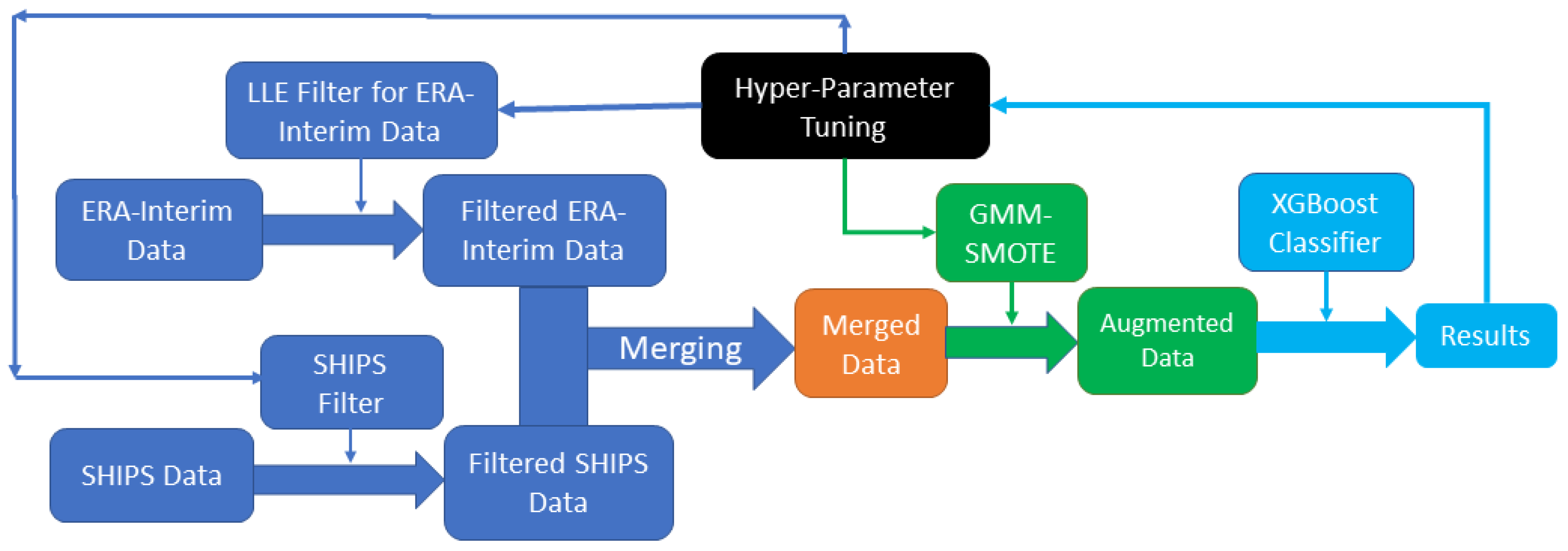
As in WY21 for the COR-SHIPS model, importance scores based on XGBoost are used to evaluate the contributions of a specific variable. However, in the LLE-SHIPS model, the inputs to the classifier are SHIPS variables and LLE-based derived variables, lle1, lle2, …, lle90, and the importance scores are for those input variables instead of the original ERA-Interim variables. At this moment, there are no available algorithms for directly calculating the importance score for the original ERA-Interim variables from XGBoost. So instead, we tried to relate the importance score (IS) of all the lle1, …, lle90 to individual ERA parameter groups (based on correlation) in two steps. First, the XGBoost was used to evaluate the importance score for SHIPS variables and lle1 to lle90 in the same way as in the COR-SHIPS model, and then a feature permutation approach was used to evaluate the importance score for the original ERA-Interim feature space separately, based on the importance score generated from the first step.

4.3.1. Variable Importance in XGBoost

Among the 162 selected and not highly correlated variables (90 LLE variables and 72 SHIPS variables), none of the LLE variables are among the top 10 variables. The reason might be there are too many variables generated from the LLE, and having so many variables reduces the importance score for each of them. This assumption is confirmed by summing the importance score for lle1 to lle90, which is 0.4288, only a bit smaller than that of the 72 SHIPS variables (0.5712). Seven of the ten most important variables are the same as that of WY21, and the three new members are TWXC, REFC, and TGRD (original abbreviations used in SHIPS are used here; readers are referred to SHIPS documentation [21] for details), which are maximum symmetric tangential wind at 850 hPa from the NCEP analysis, relative eddy momentum flux convergence, and the magnitude of the temperature gradient between 850 and 700 hPa averaged from 0 to 500 km and estimated from the geostrophic thermal wind, respectively. More details of the XGBoost scores for SHIPS features can be found in Table A1 in Appendix A.

4.3.2. Group Importance in LLE

Molnar [27] described a feature permutation approach to evaluate the importance of features on a training dataset for nonlinear models where the importance score cannot be derived easily. In that method, for the feature space in any given dataset X, f(X) is the predicted value by the classifier f, and y is the ground truth. We denote that the loss of the classifier is L(y, f(X)). Then, for each feature in the feature space X, permute its value to zero for all the observations while keeping other features unchanged (represented as X p e r m u t e ). Finally, the difference between the loss of the permuted feature space ( X p e r m u t e ) and the original loss is calculated for each feature, and the difference is used as its importance.
Although feature permutation is an efficient approach to evaluate the feature importance for different models, especially for a black-box model such as LLE, Molnar [27] also indicates that the permutated feature importance could be biased by the highly correlated features. For example, if we evaluate the importance score for each of the 2072 variables, the result, i.e., the importance score, is not accurate due to the existence of the highly correlated variables because they could influence each other. Similar to the removal of highly correlated variables in the SHIPS data filter (WY21), pairwise correlations of all the 2072 features are calculated. For a given feature, all other features with a correlation higher than a predefined threshold, 0.8, are grouped together, and a filtering process removes any duplications and keeps a feature only once in the whole list. This process results in 135 groups, and then an importance score is calculated for each group by permuting all features in that group simultaneously.
The group-level importance score is calculated specifically as follows:
Given f: trained model; X: original feature space; y: ground truth; L(y, f(X)): loss between the ground truth and the predicted value by the classifier.
1.
Calculate I m p o r t a n c e L L E _ T o t a l as the sum of the importance score of lle1 to lle90 derived from XGBoost; here, it is 0.4288.
2.
Calculate the original model error L(y, f).
3.
For each group g:
(a)
Generate feature matrix X p e r m u t e by setting features in that group to 0, which breaks the corresponding correlation between all the features.
(b)
Calculate error L(y, f( X p e r m u t e )).
(c)
Estimate the importance for the group imp = L(y, f( X p e r m u t e )) − L(y, f).
(d)
Associate the i m p g score to the group g.
(e)
Negative importance is set to 0.
4.
Group importance scores are rescaled as attributing the total important scores by LLE variables based on the ratio of loss of a particular group to the total loss (sum of all group losses), and the specific calculation is:
I m p g r o u p = I m p o r t a n c e L L E _ T o t a l i m p g r o u p / g   f o r   a l l   t h e   g r o u p s   i m p g
With the final scaling procedure on the I m p o r t a n c e L L E _ T o t a l , the group importance scores could be directly compared with those of the SHIPS features. Based on the above algorithm, the importance score for each group is calculated, and groups with the top five important scores are list in Table 7. Intuitively, turning more variables to zero could reduce the model’s performance more than turning fewer variables to zero because changing more variables is likely to alternate the model’s performance more. However, Table 7 shows that three of top five groups contain less than 15 variables while the largest group size is 309, and that indicates that the three groups with few variables play a more important role in RI prediction than the other groups, especially the groups with substantially more variables. The details of the top five groups are displayed in Supplementary Material Table S1.
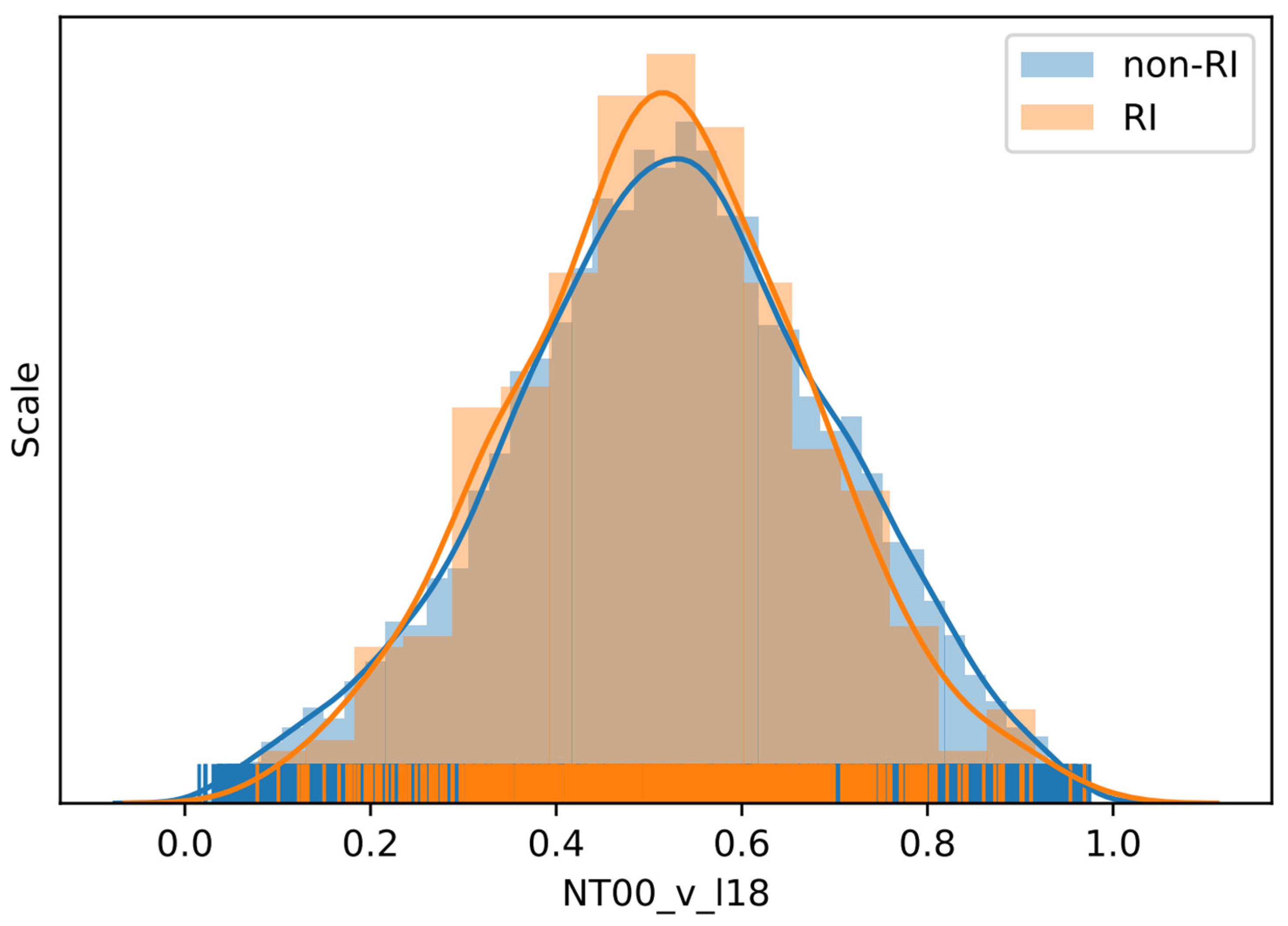
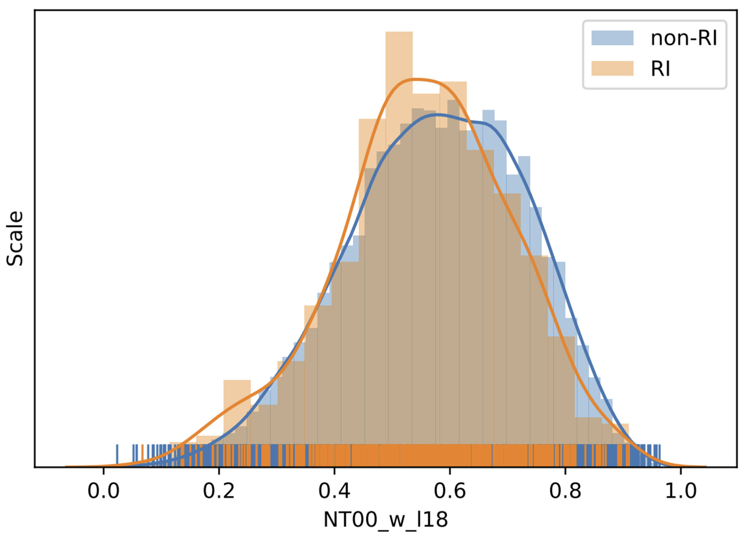
Group 49 (G49) has the highest IS, 0.023614, and it has five variables, NT06_v_l17, NT00_v_l17, NT12_v_l18, NT06_v_l18, and NT00_v_l18, which indicates that the northward wind speed on level 17 (450 hPa) at 6 h before and at present, together with level 18 (400 hPa) at 12 h before, 6 h before, and at present are important in RI prediction. The reason could be that the northward wind speed in 400 and 450 hPa changes faster than that of other levels when the RI starts to occur. We can also find that both 6 h before and the present northward wind speed are important at 400 and 450 hPa, while 12 h before only appears in 400 hPa. The result indicates that the northward wind speed in 400 and 450 hPa starts to change immediately 6–12 h before the occurrence of RI. To see the influence of this group of variables, the distributions of the meridional wind speed at 400 hPa at TC time (NT00_v_l18) for RI and non-RI instances are displayed in Figure 2. The results do not show any substantial differences between the RI and non-RI distributions. One may notice that the RI instances are more concentrated around the mean than that of the non-RI instances. Correspondingly, non-RI instances demonstrate the heavy tails, but it may simply be due to the large number of non-RI instances. Some simple quantitative statistics of the RI instances and non-RI instances over variable NT00_v_l18 are displayed in Table 8. The higher standard deviation and interquartile range confirm that the distribution of non-RI instances is flatter than that of RI instances. Since the mid-layer velocity is closely related to the movement of TCs, this importance of NT00_v_l18 says that the meridional motion of TC affects RI. This is not unexpected because storm speed was used in the seminal RI study by KD03. Intuitively, a smaller meridional speed means TCs move northward slower and have more time to obtain more energy than those moving fast in that direction. The numbers confirmed the argument because the mean and median meridional speeds for RI cases are smaller than those for non-RI cases, but the median difference is not statistically significant with the Mann–Whitney test (Table 8).
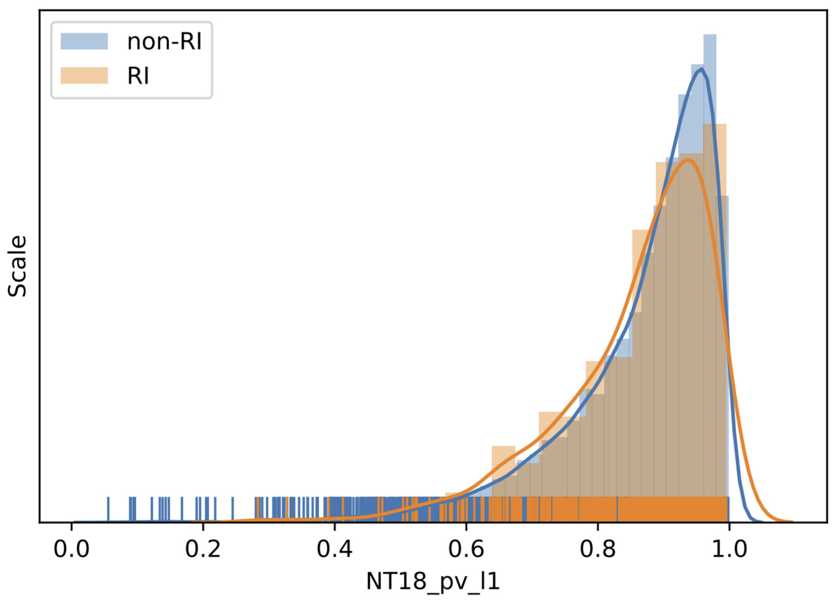
The second most important group, the G88 with an IS of 0.021988, only has one variable, NT18_pv_l1, and the potential vorticity is at 18 h before on the first level (1000 hPa). The importance score for NT18_pv_l1 is even 17% higher than that for the most important variable in Table A1, BD12 with a 0.0188 score, which is also the highest importance for a single variable. This result proved that our AI system could identify important features, which may not be in the commonly used dataset, such as the SHIPS database. However, the role of pv in RI was identified by others already (e.g., [28,29]). Tsujino and Kuo [28] detailed the changes of pv during the RI of Super Typhoon Haiyan (2013) with numerical simulation. They emphasized the pv increasing at around 3–5 km height at the beginning stage of the RI. Carefully checking their results (Figure 2b,c), one can find the pv actually increases simultaneously around the sea level in the 20–40 km range from the center, which is the same as what we identified here by the NT18_pv_l1. Figure 2 and Figure 3 display the distribution of potential vorticity at 1000 hPa for RI and non-RI instances, respectively, and the corresponding quantitative statistics are also listed in Table 8. The means and medians of RI and non-RI cases follow the same pattern. That is, the non-RI medians are higher than the RI medians, and the pv median difference is statistically significant at the 0.05 significance level. The result is consistent with Rogers et al. [30], who composited airborne Doppler radar data for intensifying and stable TCs and found the mean pv with intensifying TCs is significantly lower than that for TCs in a steady state.
All level one pv (three of them) are grouped in G63 with importance scores (IS) (0.010746). All level two pv are in G55 with four members and 0.004744 IS. All other pv are in G4 with 140 members but IS being only 0.006264. Those numbers illustrated that only lower layer pv affects the RI process.
The third most important group is G1, which has 309 features in the group, and with an IS of 0.019687. Since all types of ERA-Interim variables are included in the group, it is difficult to trace back which variable is more important.
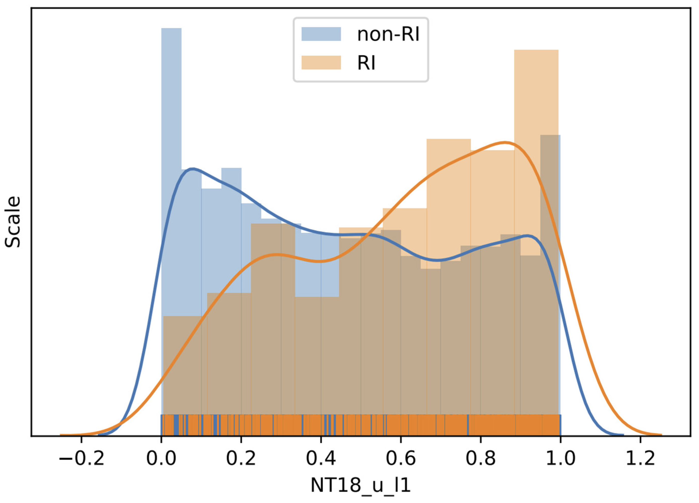
The fourth most important group is G29, which has an IS of 0.019662, very close to the third highest value, and consists of 11 variables, i.e., NT18_u_l1, NT12_u_l1, NT06_u_l1, NT00_t_l10, NT00_u_l16, NT00_u_l17, NT06_u_l17, NT12_u_l17, NT18_u_l18, NT12_u_l18, and NT18_u_l17. We can find that most of the variables in the group are u, the zonal wind speed. It is interesting to note that the zonal speeds at 1000 hPa (level 1) 6–18 h before the current time are highly correlated with the corresponding speeds at 450 hPa (level 17) and 400 hPa (level 18). As we carried out before, we chose NT18_u_l1, the zonal speed at 1000 hPa 18 h before the current time, as the group representative and displayed the value distributions for RI and non-RI cases (Figure 4) and quantitative statistics (Table 8). The distributions for RI and non-RI instances are substantially different, unlike the cases for NT00_v_l18 and NT18_pv_l1. Both of the distributions are non-Gaussian and with minor second modes. However, more RI instance values are close to one while more non-RI instance values approach zero. From Table 8, we can find lower 25 percentile, median, and 75 percentile of non-RI instances than those of RI instances. Similarly, the p value of NT18_u_l1 indicates that the median difference between RI and non-RI instances is statistically significant.
Similar to the meridional speeds (G49) but slightly different, the eastward wind speeds at level 17 (450 hPa) and 18 (400 hPa) in G29 also play an important role in RI prediction. In addition to the 400 and 450 hPa eastward wind speed, the eastward wind at 1000 hPa at 6, 12, and 18 h is also in G29. Wang et al. [10] found that “low-level shear between 850 (or 700) and 1000 hPa is more negatively correlated with TC intensity change than any deep-layer shear during the active typhoon season”, which matches our findings that eastward wind speed, related to the VWS, at 1000 hPa is significant in RI prediction. Additionally, we also recognize that the mid-level (400 and 450 hPa) eastward wind speed (possibly via VWS) is important to TC intensity change. One exception variable in this group is the temperature at 775 hPa, NT00_t_l10; although it is highly correlated with u in terms of value, it is possibly misplaced in the group because there is only one t variable in the group.
The fifth most important score is 0.01728 with G3, consisting of 148 w (the pressure vertical velocity) variables. In other words, all w components for four times and 37 levels are all grouped here. In the warm core of a TC, the upward motions near the center as part of the secondary circulation (also with low-level inflow and upper-level outflow) show strong correlations among the motion at different times (from 18 h before to current time) for all vertical layers. This strong linear relationship is partially due to the relative uniform distribution of the vertical velocity across most of atmosphere [31] and partially due to the averaging process in the 240 km × 240 km boxes, which smoothed out all the differences between the eyes and eyewalls [32]. Rogers et al. [30] found that the eyewall vertical velocity is significantly higher in intensifying (IN) cases than that in steady state cases. While downward motion was identified by Rogers et al. [30] very close to TC centers in IN cases, on average the results there show that stronger upward eyewall vertical velocity is in favor to RI, possibly due to the stronger secondary circulation. Similar to previous figures, Figure 5 displays the distribution of pressure vertical velocity at 400 hPa (level 18) for RI and non-RI instances, respectively, and we can find the distribution of RI more right skewed than that of non-RI instances. This is because the pressure vertical velocity is of negative values for upward moving air, and the finding is confirmed by the corresponding quantitative statistics listed in Table 8, with the RI mean and median being smaller than the non-RI mean and median.
This result seems to be not consistent with what was found with the SHIPS data. In the SHIPS database, variables O500 and O700 for the pressure vertical velocity (w) at 500 and 700 hPa are highly correlated (Table A1 in WY21) and are ranked only 72 with a 0.0058 importance score (see Table A1). The contributions from all the w components together are almost three times more important than the single w representative, O500, as measured by IS here. One plausible interpretation is that differences among the 148 variables are smoothed out, and the higher IS contribution is simply due to the much higher number of actual variables than a single representative variable. More research is needed to figure out the details for the contribution of the pressure vertical velocity to the RI process.
In sum, two out of the top five important groups, G45 and G29, contain eastward and northward wind speed variables, especially at 400, 450, and 1000 hPa. Those speeds are related to the VWS-involved wind velocity at 400, 450, and 1000 hPa pressure levels, which are known to play a significant role in RI prediction, as revealed by Wang et al. [10]. Another group, G3, only contains the pressure vertical velocity, which indicates that vertical pressure speed is critical in RI prediction. Other than the O500 and O700 included in the SHIPS database, it is necessary to dig out details of the pressure vertical velocity contribution to RI at different pressure levels without heavy grouping.
Here, we derive the group level importance score for ERA-Interim variables. Although the AI system consists of too many components so that the score is not 100% accurate, the system is still able to identify useful features in addition to the SHIPS database.

4.4. Model Comparison

The COR-SHIPS model, as a baseline for a model with modern AI techniques and SHIPS data only, displayed substantial improvements in RI prediction vs. other existing research models (WY21) [15]. Here, we compare the performance of the LLE-SHIPS model against that of the COR-SHIPS model in Table 9. The kappa, PSS, and POD are improved by 26.6%, 8.4%, and 2.4%, while FAR decreases 27.2%, respectively. If we go back to the models cited in WY21, the improvements on POD are 23.8% and 53.1% over Yang [7] and Kaplan et al. [5], respectively, with 36.4% and 45.2% FAR reduction.
DeMaria et al. [18] recently summarized the NHC operational RI prediction performance with various models including statistical–dynamical and numerical simulation (regional dynamical and global dynamical) models. Two regional dynamical models, HWFI and HMNI, give the 30 kt/24 h RI POD 21% and 10%, respectively, with a 50% FAR value. The official NHC prediction (OFCL) for the 2016–2020 Atlantic RI prediction is POD, 14% and FAR, 32%. It should be pointed out that it is not fair to compare the operational prediction with our research analysis based on the historical data, and the former is much more difficult.

4.5. Feature Importance Comparison between Previous Studies and This Study

Compared to the COR-SHIPS model, the LLE-SHIPS model not only employs SHIPS parameters but also ERA-Interim near-center parameters for predicting RI. We divided the ERA-Interim parameters into different groups with highly correlated parameters to evaluate the group importance instead of evaluating the importance for each parameter. Based on the top five important groups, we found that wind speed, especially at 400, 450, and 1000 hPa, plays a significant role in RI prediction. Another piece of important information we obtained, potential vorticity at 1000 hPa (NT18_pv_l1), is more important than the most important SHIPS variable, BD12. Finally, all the variables of vertical pressure speed are highly correlated with each other and were found to be important in RI prediction.

5. Conclusions

To improve RI prediction with modern techniques, we constructed a well-tailored artificial intelligence (AI) system, which adopts data filters, oversamples RI instances, employs a powerful classifier, and tunes involved hyperparameters. The first example is the COR-SHIPS model, which fully depends on SHIPS data but with improved RI prediction performance (WY21). However, the mechanism of the tropical cyclone RI is unknown, and important variables may not be included in the SHIPS dataset. Therefore, under the same framework, this study extends the COR-SHIPS model to include the ECMWF ERA-Interim reanalysis data in hopes to identify RI-related features beyond SHIPS. To overcome the extremely high dimensions with the multi-level gridded data arrays, an automatic feature extraction approach, local linear embedding (LLE), was used to extract features from near-center data (small scale) to create the LLE-SHIPS model.
The entire dataset is split into training/validation and test sets, where the former is used to fit our model and to tune the hyperparameters, and the latter is used for the performance evaluation and comparison. The performance of our model on the test data showed improvement in the RI prediction with hyperparameter tuning.
It was found that our LLE-SHIPS model outperforms the COR-SHIPS model in terms of kappa, PSS, and POD, being improved by 26.6%, 8.4%, and 2.4% while FAR decreases 27.2%, respectively, and we believe the improvement by this work is substantial. Of course, the reanalysis is not available for real forecasting, but the features identified with the reanalysis could be derived from forecasting model data as in the so-called statistical–dynamical models such as SHIPS. The significant improvement made by the model also challenges the mainstream point of selecting only a few variables fitting in the simple model for the prediction, i.e., involving more variables in the complicated model with high penalty terms is better than a simple model with few variables.
The variable importance was also evaluated, and top ten factors are actually from SHIPS datasets, similar to those with the COR-SHIPS model. The additional significant variables identified by the LLE-SHIPS model are the wind speed, especially at 400 and 450 hPa, potential vorticity at 1000 hPa, pressure vertical velocity in the near center, and those parameters could help to understand the mechanism of the TC intensification.
Although we can trace back the importance to the parameter level with limited accuracy via the LLE technique, accurately tracing back to the feature level importance is still challenging in the AI community. This is because, with so many non-linear transforms in the complicated machine learning model structure, no one can easily tell what is going on [27]. The next step is to look for an approach that better identifies the feature importance and even leverages the updated ECMWF reanalysis data, the ERA-5 dataset [33]. Moreover, in addition to the near-core variables used in the LLE-SHIPS model, we should also explore the large-scale information in the ERA-Interim data influencing the RI prediction, potentially with oceanic components.

Supplementary Materials

The following supporting information can be downloaded at: https://0-www-mdpi-com.brum.beds.ac.uk/article/10.3390/atmos13050643/s1, Table S1: Detail of the LLE-based feature groups with the top five importance scores.

Author Contributions

Conceptualization, Y.W. and R.Y.; methodology, Y.W.; software, Y.W.; validation, Y.W.; formal analysis, Y.W.; investigation, Y.W. and R.Y.; resources, Y.W.; data curation, Y.W.; writing—original draft preparation, Y.W.; writing—review and editing, Y.W., R.Y., J.K., I.G. and O.G.; visualization, Y.W.; supervision, R.Y., J.K., I.G. and O.G. All authors have read and agreed to the published version of the manuscript.

Funding

This research received no external funding.

Institutional Review Board Statement

Not applicable.

Data Availability Statement

The SHIPS data used in this study are publicly available online at http://rammb.cira.colostate.edu/research/tropical_cyclones/ships/developmental_data.asp (last accessed on 4 March 2022). The ERA-Interim data are available at https://www.ecmwf.int/en/forecasts/datasets/reanalysis-datasets/era-interim (last accessed on 4 March 2022).

Acknowledgments

The authors thank the SHIPS group and the ERA-Interim group for making the SHIPS data and ERA-Interim data available. The authors also thank three anonymous reviewers, whose comments helped to improve the quality of the manuscript.

Conflicts of Interest

The authors declare no conflict of interest.

Appendix A

Table A1. LLE-SHIPS model feature importance score (IS) and its ranking.
RankVariableISRankVariableISRankVariableIS
1BD120.01955lle20.0064109lle70.0047
2VMAX0.01756IR00_200.0064110lle390.0047
3DTL0.01457NSST0.0063111lle290.0047
4SHRD0.01358Z8500.0062112lle110.0046
5TWXC0.01259NTFR0.0062113IRM3_170.0046
6G1500.01160IR00_140.0061114lle440.0046
7VMPI0.01161NOHC0.0061115lle120.0046
8REFC0.01162lle890.0061116lle420.0046
9TGRD0.01163IRM3_140.006117lle270.0045
10IRM1_50.01164lle710.006118lle740.0045
11IR00_120.01165lle30.006119lle220.0045
12V3000.01166lle520.006120lle620.0044
13VVAC0.01167lle190.0059121lle820.0044
14G2000.0168lle510.0059122PCM30.0044
15PEFC0.0169lle720.0059123lle470.0044
16MTPW_10.0170IR00_170.0059124lle320.0044
17XDTX0.0171lle40.0059125lle430.0043
18PSLV_10.0172O5000.0058126lle800.0043
19T1500.0173lle530.0058127lle830.0043
20CFLX0.00974V8500.0058128lle310.0043
21HIST_20.00975TLAT0.0058129lle60.0042
22HE070.00976lle660.0057130lle150.0042
23SHTS0.00977lle300.0057131lle700.0042
24PSLV_30.00978RHMD0.0056132lle630.0042
25SHTD0.00979lle600.0056133lle380.0042
26G2500.00980lle160.0056134lle460.0042
27CD260.00981IR00_30.0055135lle230.0042
28lle840.00882lle760.0055136lle340.0041
29EPSS0.00883lle570.0055137PENV0.0041
30R0000.00884lle690.0054138lle580.0041
31SDDC0.00885lle540.0054139lle360.004
32IRM3_190.00886PC000.0054140lle590.0039
33RD260.00887lle80.0053141lle680.0039
34PW080.00788lle770.0052142lle650.0039
35SHRS0.00789IRM3_110.0052143lle250.0039
36NDTX0.00790IRM1_140.0052144lle280.0039
37lle750.00791lle330.0052145lle450.0038
38jd0.00792lle100.0051146lle140.0038
39TADV0.00793IRM1_170.0051147lle640.0038
40NDFR0.00794lle550.0051148lle610.0038
41E0000.00795lle560.0051149lle410.0037
42HIST_90.00796T2500.0051150lle850.0037
43PSLV_40.00797lle260.005151lle900.0037
44MTPW_190.00798lle810.005152lle880.0036
45IRM1_160.00799lle730.005153lle790.0036
46PW140.007100XDML0.0049154lle870.0035
47OAGE0.007101lle130.0049155lle50.0035
48lle780.007102D2000.0049156lle350.0035
49XD180.007103lle170.0048157lle180.0034
50lle10.007104lle370.0048158lle670.0034
51lle490.007105lle210.0048159lle860.0034
52lle240.007106lle200.0048160lle500.0032
53PCM10.007107lle480.0048161lle400.003
54ND200.007108lle90.0048162HIST_160.0018

References

  1. Dong, J.; Liu, B.; Zhang, Z.; Wang, W.; Mehra, A.; Hazelton, A.T.; Winterbottom, H.R.; Zhu, L.; Wu, K.; Zhang, C.; et al. The Evaluation of Real-Time Hurricane Analysis and Forecast System (HAFS) Stand-Alone Regional (SAR) Model Performance for the 2019 Atlantic Hurricane Season. Atmosphere 2020, 11, 617. [Google Scholar] [CrossRef]
  2. Kaplan, J.; DeMaria, M. Large-scale characteristics of rapidly intensifying tropical cyclones in the North Atlantic basin. Weather Forecast. 2003, 18, 1093–1108. [Google Scholar] [CrossRef] [Green Version]
  3. DeMaria, M.; Mainelli, M.; Shay, L.K.; Knaff, J.; Kaplan, J. Further improvements to the statistical hurricane intensity prediction scheme (SHIPS). Weather Forecast. 2005, 20, 531–543. [Google Scholar] [CrossRef] [Green Version]
  4. Yang, R.; Tang, J.; Kafatos, M. Improved associated conditions in rapid intensifications of tropical cyclones. Geophys. Res. Lett. 2007, 34, L20807. [Google Scholar] [CrossRef] [Green Version]
  5. Kaplan, J.; Rozoff, C.M.; DeMaria, M.; Sampson, C.R.; Kossin, J.; Velden, C.S.; Cione, J.J.; Dunion, J.P.; Knaff, J.; Zhang, J.; et al. Evaluating environmental impacts on tropical cyclone rapid intensification predictability utilizing statistical models. Weather Forecast. 2015, 30, 1374–1396. [Google Scholar] [CrossRef]
  6. Kaplan, J.; DeMaria, M.; Knaff, J. A revised tropical cyclone rapid intensification index for the Atlantic and eastern North Pacific basins. Weather Forecast. 2010, 25, 220–241. [Google Scholar] [CrossRef]
  7. Yang, R. A Systematic Classification Investigation of Rapid Intensification of Atlantic Tropical Cyclones with the SHIPS Database. Weather Forecast. 2016, 31, 495–513. [Google Scholar] [CrossRef]
  8. Mercer, A.E.; Grimes, A.D.; Wood, K.M. Application of Unsupervised Learning Techniques to Identify Atlantic Tropical Cyclone Rapid Intensification Environments. J. Appl. Meteorol. Climatol. 2021, 60, 119–138. Available online: https://journals.ametsoc.org/view/journals/apme/60/1/jamc-d-20-0105.1.xml (accessed on 3 March 2021). [CrossRef]
  9. Su, H.; Wu, L.; Jiang, J.H.; Pai, R.; Liu, A.; Zhai, A.J.; Tavallali, P.; DeMaria, M. Applying satellite observations of tropical cyclone internal structures to rapid intensification forecast with machine learning. Geophys. Res. Lett. 2020, 47, e2020GL089102. [Google Scholar] [CrossRef]
  10. Wang, Y.; Rao, Y.; Tan, Z.-M.; Schönemann, D. A statistical analysis of the effects of vertical wind shear on tropical cyclone intensity change over the western North Pacific. Mon. Weather Rev. 2015, 143, 3434–3453. [Google Scholar] [CrossRef]
  11. Qian, Y.-K.; Liang, C.-X.; Peng, S.; Chen, S.; Wang, S. A Horizontal Index for the Influence of Upper-Level Environmental Flow on Tropical Cyclone Intensity. Weather. Forecast. 2016, 31, 237–253. [Google Scholar] [CrossRef]
  12. Wang, Z. What is the key feature of convection leading up to tropical cyclone formation? J. Atmos. Sci. 2018, 75, 1609–1629. [Google Scholar] [CrossRef]
  13. Astier, N.; Plu, M.; Claud, C. Associations between tropical cyclone activity in the Southwest Indian Ocean and El Niño Southern Oscillation. Atmos. Sci. Lett. 2015, 16, 506–511. [Google Scholar] [CrossRef] [Green Version]
  14. Ferrara, M.; Groff, F.; Moon, Z.; Keshavamurthy, K.; Robeson, S.M.; Kieu, C. Large-scale control of the lower stratosphere on variability of tropical cyclone intensity. Geophys. Res. Lett. 2017, 44, 4313–4323. [Google Scholar] [CrossRef] [Green Version]
  15. Wei, Y.; Yang, R. An Advanced Artificial Intelligence System for Investigating Tropical Cyclone Rapid Intensification with the SHIPS Database. Atmosphere 2021, 12, 484. [Google Scholar] [CrossRef]
  16. SHIPS. 2018a: SHIPS Statistical Tropical Cyclone Intensity Forecast Technique Development, Developmental Data. Available online: http://rammb.cira.colostate.edu/research/tropical_cyclones/ships/developmental_data.asp (accessed on 3 February 2020).
  17. SHIPS. 2018b. Available online: http://rammb.cira.colostate.edu/research/tropical_cyclones/ships/docs/AL/lsdiaga_1982_2017_sat_ts.dat (accessed on 3 February 2020).
  18. DeMaria, M.; Franklin, J.L.; Onderlinde, M.J.; Kaplan, J. Operational Forecasting of Tropical Cyclone Rapid Intensification at the National Hurricane Center. Atmosphere 2021, 12, 683. [Google Scholar] [CrossRef]
  19. Dee, D.P.; Uppala, S.M.; Simmons, A.J.; Berrisford, P.; Poli, P.; Kobayashi, S.; Andrae, U.; Balmaseda, M.A.; Balsamo, G.; Bauer, P.; et al. The ERA-Interim reanalysis: ConFiguration and performance of the data assimilation system. Q. J. R. Meteorol. Soc. 2011, 137, 553–597. [Google Scholar] [CrossRef]
  20. Molinari, J.; Vollaro, D. Vollaro, External influences on hurricane intensity. Part I: Outflow layer eddy angular momentum fluxes. J. Atmos. Sci. 1989, 46, 1093–1105. [Google Scholar] [CrossRef] [Green Version]
  21. SHIPS. 2018c. Available online: http://rammb.cira.colostate.edu/research/tropical_cyclones/ships/docs/ships_predictor_file_2018.doc (accessed on 3 February 2020).
  22. Pasch, R.J.; Blake, E.S.; Cobb, H.D., III; Roberts, D.P.; National Hurricane Center. Tropical Cyclone Report: Hurricane Wilma: 15–25 October 2005. 2006. Available online: https://www.nhc.noaa.gov/data/tcr/AL252005_Wilma.pdf (accessed on 3 March 2022).
  23. Yang, R.; Tan, J.; Kafatos, M. A Pattern Selection Algorithm in Kernel PCA Applications. In Proceedings of the First International Conference on Software and Data Technologies, Setubal, Portugal, 11–14 September 2006; pp. 195–202. [Google Scholar]
  24. Roweis, S.T.; Saul, L.K. Nonlinear dimensionality reduction by locally linear embedding. Science 2000, 290, 2323–2326. [Google Scholar] [CrossRef] [Green Version]
  25. Géron, A. Hands-On Machine Learning with Scikit-Learn and TensorFlow: Concepts, Tools, and Techniques to Build Intelligent Systems; O’Reilly Media, Inc.: Sebastopol, CA, USA, 2017. [Google Scholar]
  26. Ginsburg, S.B.; Lee, G.; Ali, S.; Madabhushi, A. Madabhushi, Feature importance in nonlinear embeddings (FINE): Applications in digital pathology. IEEE Trans. Med. Imaging 2016, 35, 76–88. [Google Scholar] [CrossRef]
  27. Molnar, C. Interpretable Machine Learning: A Guide for Making Black Box Models Explainable. Christoph Molnar Leanpub. 2019. Available online: https://christophm.github.io/interpretable-ml-book/ (accessed on 3 February 2020).
  28. Tsujino, S.; Kuo, H.-C. Potential Vorticity Mixing and Rapid Intensification in the Numerically Simulated Supertyphoon Haiyan (2013). J. Atmos. Sci. 2020, 77, 2067–2090. [Google Scholar] [CrossRef] [Green Version]
  29. Martinez, J.; Bell, M.M.; Rogers, R.F.; Doyle, J.D. Axisymmetric Potential Vorticity Evolution of Hurricane Patricia (2015). J. Atmos. Sci. 2019, 76, 2043–2063. [Google Scholar] [CrossRef] [Green Version]
  30. Rogers, R.; Reasor, P.; Lorsolo, S. Airborne Doppler Observations of the Inner-Core Structural Differences between Intensifying and Steady-State Tropical Cyclones. Mon. Weather Rev. 2013, 141, 2970–2991. [Google Scholar] [CrossRef]
  31. Frank, W.M. The Structure and Energetics of the Tropical Cyclone I. Storm Structure. Mon. Weather Rev. 1977, 105, 1119–1135. [Google Scholar] [CrossRef]
  32. Jorgensen, D.F. Mesoscale and Convective-Scale Characteristics of Mature Hurricanes. Part I: General Observations by Research Aircraft. J. Atmos. Sci. 1984, 41, 1268–1286. [Google Scholar] [CrossRef] [Green Version]
  33. Malakar, P.; Kesarkar, A.; Bhate, J.; Singh, V.; Deshamukhya, A. Comparison of reanalysis data sets to comprehend the evolution of tropical cyclones over North Indian Ocean. Earth Space Sci. 2020, 7, e2019EA000978. [Google Scholar] [CrossRef] [Green Version]
Figure 1. The LLE-SHIPS model structure.
Atmosphere 13 00643 g001
Figure 2. The value distribution for variable NT00_v_l18 (current 400 hPa meridional wind speed) over RI and non-RI instances. The x-axis represents the scaled value of the variable, the bar chart in the y-axis represents relative frequency of the values falling in certain ranges, and the curves are the smoothed distribution via the kernel density estimation. The smoothed lines out of interval [0, 1] do not represent any valid value.
Atmosphere 13 00643 g002
Figure 3. Same as Figure 2 but for variable NT18_pv_l1 (potential vorticity 18 h before current time at 1000 hPa).
Atmosphere 13 00643 g003
Figure 4. Same as Figure 2 but for variable NT18_u_l1 (zonal wind speed 18 h before current time at 1000 hPa).
Atmosphere 13 00643 g004
Figure 5. Same as Figure 2 but for variable NT00_w_l18 (pressure vertical velocity at 0 h at 400 hPa).
Atmosphere 13 00643 g005
Table 1. Variable names, abbreviations (abbr.), units, and description for the 14 variables in the ERA-Interim pressure level dataset.
Variable NameAbbr.UnitDescription
Fraction of cloud coverccpercentageHorizontal fraction of the grid box covered by cloud
Cloud ice water contentciwckg kg−1Grid-box mean specific cloud ice water content (mass of condensate/mass of moist air)
Cloud liquid water contentclwckg kg−1Grid-box mean specific cloud liquid water content (mass of condensate/mass of moist air)
Divergenceds−1Relative divergence
Geopotentialzm2 s−2At the surface: orography
Vertical velocitywPa s−1Pressure vertical velocity dp/dt. In the model equations it is usually denoted by the Greek letter omega
Ozone mass mixing ratioo3kg kg−1Mass mixing ratio of ozone
Potential vorticitypvK m2 kg−1s−1The ability of air to rotate in the atmosphere. “Conservation equation directly ties together the dynamics and the heating” [20]
Relative humidityrpercentageRelative humidity is defined with respect to saturation of the mixed phase, i.e., with respect to saturation over ice below −23 °C and with respect to saturation over water above 0 °C. In the regime in between, a quadratic interpolation is applied
Specific humidityqkg kg−1Grid-box mean (mass of water vapor/mass of moist air)
TemperaturetKTemperature
U component of windum s−1West-to-east flow (eastward wind)
V component of windvm s−1South-to-north flow (northward wind)
Vorticity (relative)vos−1Measure of the rotation of air in the horizontal
Table 2. The performance for models with different sets of values of the hyperparameters, no_dimension and no_neighbors, on training dataset.
Kappa ScoreRankNo_DimensionNo_Neighbors
0.29719015
0.29528915
0.2938713
0.28749014
0.28258015
Table 3. The number of minority and total cases, and the imbalance rate (with population RI ratio at 5.1%) for the 5 clusters generated by GMM.
Cluster12345Total
# RI Instance1962611239150523
# Total Instance3048185810781608259310,185
Imbalance Rate1.2860.2802.0780.4851.1571
Table 4. The hyperparameters for GMM-SMOTE (excluding n_cluster) and XGBoost (excluding decision threshold) and their corresponding values used for the model. For the definition of the hyperparameters, readers are referred to WY21 [15].
Hyperparameters NameValue
m_neighbors8
k_neighbors12
shrinkage0.21
n_estimators731
subsample0.85
colsample_bytree0.8
reg_alpha0.1
reg_lambda0.5
gamma0
min_child_weight1.4
max_depth10
Table 5. Confusion matrix values after (before) hyperparameter tuning with the test data.
Predicted RIPredicted Non-RIActual
Actual RI40 (20)55 (75)95
Actual non-RI33 (11)1469 (1491)1502
Predicted73 (31)1524 (1566)
Table 6. Performance comparisons. MB and MA denote the models before and after the hyperparameters in GMM-SMOTE and XGBoost are tuned.
ModelKappaPSSPODFAR
MB0.2970.2030.2110.355
MA0.4480.3990.4210.452
Improvement MB50.8%96.6%99.5%27.3%
Table 7. ERA-Interim variable groups with top 5 importance scores. The values of group number (group), the number of variables in the group (group size), and the importance score (IS) are given.
GroupGroup SizeIS
4950.023614
8810.021988
13090.019687
29110.019662
31480.017280
Table 8. Basic statistic values for features NT00_v_l18, NT18_pv_l1, NT18_u_l1, and NT00_w_l18 for RI and non-RI (NRI) instances, respectively. The p-values are for the Mann–Whitney test against the same median in each case.
Variable NT00_v_l18NT18_pv_l1NT18_u_l1NT00_w_l18
RINRIRINRIRINRIRINRI
mean0.5130.5210.8570.8670.5990.4630.5520.577
std0.1620.1780.1170.1170.2810.3070.1530.155
25%0.4110.4030.7990.8180.3620.1850.4600.471
median0.5150.5240.8900.9030.6390.4410.5580.583
75%0.6230.6440.9460.9510.8440.7350.6550.692
p-value0.11330.00472 × 10−230.0002
Table 9. Performance comparison between the model developed in this study and the baseline COR-SHIPS model. The values for COR-SHIPS model are copied from Table 9 of WY21.
ModelKappaPSSPODFAR
COR-SHIPS0.3540.3680.4110.621
LLE-SHIPS0.4480.3990.4210.452
Improvement COR-SHIPS26.6%8.4%2.4%−27.2%
Publisher’s Note: MDPI stays neutral with regard to jurisdictional claims in published maps and institutional affiliations.

