Article

A Climatology of Mesoscale Convective Systems in Northwest Mexico during the North American Monsoon

by
Omar Ramos-Pérez
1,*,
David K. Adams
2,
Carlos A. Ochoa-Moya
2 and
Arturo I. Quintanar
2
1
Posgrado en Ciencias de la Tierra, Universidad Nacional Autónoma de Mexico, Mexico City 04510, Mexico
2
Instituto de Ciencias de la Atmósfera y Cambio Climático, Universidad Nacional Autónoma de México, Mexico City 04510, Mexico
*
Author to whom correspondence should be addressed.
Submission received: 4 March 2022 / Revised: 17 April 2022 / Accepted: 18 April 2022 / Published: 22 April 2022
(This article belongs to the Special Issue Moist Atmospheric Convection)

Abstract

:
Mesoscale Convective Systems (MCS) may vary greatly with respect to their morphology, propagation mechanism, intensity, and under which synoptic-scale conditions as a function of topographic complexity. In this study, we develop a long-term climatology of MCS during the North American Monsoon focusing on MCS morphology, lifecycle, and intensity as well as possible propagation mechanisms. We employ an MCS tracking and classification technique based on 23 years (1995 to 2017) of GOES IR satellite data. MCS intensity is also gauged with 7 years (2011 to 2017) of Vaisala GLD360 lightning data and, finally, monthly and interannual variability in synoptic conditions are examined with ERA5 reanalysis data. Our results based on 1594 identified MCS reveal that 98% are morphologically classified as Persistent Elongated Convective Systems. During the 23 summers (June through September) observed, the number of MCS varied considerably, averaging 70 MCS with minimum of 41 and maximum of 94. MCS typically have an average duration of around 8 h ± with a 2 h standard deviation. Propagation speeds, estimated with Hovmöller diagrams in addition to MCS centroid initial and final position, vary slightly depending on the trajectory. A notable result suggests that MCS propagation speeds are more consistent density currents or cold pools and not gravity waves nor steering-level winds. The results of this study could also provide a dataset for examining larger-scale controls on MCS frequency in addition to assesing convective parameterization and convective-resolving models in regions of complex topography.

1. Introduction

Understanding the organization, propagation mechanisms, and intensity of Mesoscale Convective Systems (MCS), as well as their representation in numerical models have been a fundamental challenge in the atmospheric sciences for decades. Definitionally, MCS are organized cumulonimbus clouds in a single cohesive entity with precipitation occurring on spatial scales of at least 100 km in a given direction and a lifecycle of several hours to one day [1,2]. Although MCS vary greatly morphologically, the typical morphological structure captured with radar data consists of a deep convective region of intense, but relatively brief precipitation, and a stratiform region with lighter precipitation of greater duration [3,4,5,6]. Intense MCS are associated with severe weather phenomena such as frequent lightning, hail, flash floods, strong wind gusts, and even tornadoes [7,8,9]. MCS occur across the globe in the mid-latitudes, subtropics, and tropics though the dynamical forcing mechanisms or thermodynamic conditions responsible for their formation may differ greatly [10,11]. Given this large geographical range and frequency of occurrence, MCS also play a fundamental role within the climate system vertically redistributing heat, water vapor, and momentum [12,13,14,15,16]. The formation of MCS typically requires sufficient atmospheric instability, substantial lower atmospheric humidity, wind shear, and some form of triggering mechanism [17,18]. In some regions, local terrestrial surface moisture may also play a role in the initiation of deep convection [19,20,21,22]. Topography can also be of fundamental import in initiating deep convective cells, their upscale growth into MCS, and propagation characteristics [8,23,24,25]. Likewise, coastal topographic configurations can greatly impact the formation and propagation of these systems. For example, the formation of off-shore convection along low-level convergence zones between the sea-breeze and monsoonal flow [26,27] or through atmospheric destabilization resulting from gravity wave propagation [28,29,30] are related to coastal topography. Understanding the effects of topography on convective initiation and organization has motivated various field campaigns; for example, the Mesoscale Alpine Programme in 1999 [31,32], the Convective and Orographically induced Precipitation Study (COPS) in 2007 [33,34], the North American Monsoon GPS Transect Experiment [35], Remote sensing of Electrification, Lightning, And Mesoscale/microscale Processes with Adaptive Ground Observations (RELAMPAGO) and Cloud, Aerosol, and Complex Terrain Interactions (CACTI) in 2018–2019 [36,37,38].
An additional challenging aspect of MCS evolution, difficult to replicate in numerical models, is their variability in morphology as a function of environmental conditions [39,40,41]. MCS morphology, based on cirrus shield shape and corresponding shield areal extent, has been shown to be closely tied to storm severity [40,41,42,43]. For example, Mesoscale Convective Complexes (MCC) [44] have a cold cloud region (≤−52 °C) with an area ≥50,000 km2 and circular in shape while Persistent Elongated Convective Systems (PECS) [45], though similar in areal coverage, are characterized by their elongated form.
Both MCC, as well as PECS, generally occur in environmental conditions with large CAPE values, a small Lifted Index (LI), and strong vertical wind shear in the lower troposphere [40,46]. However, Jirak et al. [40] found, in the Great Plains region of the central United States, that greater than 50% of severe weather reports were associated with PECSs, although the authors pointed out that significant differences in environmental conditions were not encountered for MCC occurrence. Parker and Johnson [39] note that MCS with trailing stratiform precipitation occur in more unstable environments producing intense cold pools compared to those with parallel or leading stratiform precipitation. It should be emphasized, however, that a substantial portion of these MCS morphology studies consider regions where complex topography is not a factor.
A region where deep convective activity and MCS formation are intrinsically tied to the complex topography is that of the North American Monsoon (NAM) [47,48,49,50,51,52,53,54,55]. The initiation and upscale growth of MCS over the Sierra Madre Occidental (SMO) of northwestern Mexico is a fundamental characteristic of the NAM. MCS, which often propagate towards lower terrain, are critical for water resources [56], in addition to generating severe weather [57,58]. MCS in the NAM region have been the focus of previous studies [59,60,61,62,63]. MCS trajectories towards the Gulf of California can trigger or enhance moisture surges which penetrate northward towards southeastern California and Arizona modulating convective activity, therefore resulting in a non-local or upscale effect [63]. Hence, understanding MCS initiation and organization as well as improving their forecasting and representation in numerical weather prediction have strongly motivated NAM experimental campaigns, such as the North America Monsoon Experiment (NAME) [64,65], the Cumulus Photogrammetric, In Situ, and Doppler Observations (CuPIDO) [50], the North American Monsoon GPS Transect Experiment 2013 [35] and the NAM GPS Hydrometeorological Network 2017 [66].
In the NAM region, convective initiation typically occurs during the early afternoon over the highest elevations of the SMO [67,68,69,70] and the elevated topography of central and southern Arizona [49,71,72,73,74]. Over northwestern Mexico, given conducive, large-scale flow and thermodynamic conditions, this afternoon convective activity over the SMO can organize into MCS which often propagate towards the Gulf of California (GoC) [56,69,70,75]. In particular, an increase in mid-level easterly winds favors upscale growth and propagation [59,62,76]. Furthermore, synoptic-scale disturbances, especially inverted troughs (IVs), favor the initiation and propagation of MCS argued to result from increased upper-level divergence and associated destabilization [77], or, from the intensification of vertical wind shear [53,54,78]. Lang et al. [56] found that MCS not only progress towards the GoC (their Regime A), but also travel parallel to the GoC coastal zone (their Regime B) and there are even occasions when they propagate both along-coast and cross-coast (their Regime AB). MCS propagation speeds of ∼7 m/s, ∼10 m/s and ∼3–5 m/s are found in regimes A, B, and AB, respectively. Lang et al. [56] argue that the mechanism that best explains these propagation speeds is the occurrence of weak and shallow cold pools, not gravity waves as argued, for example, by Mapes et al. [28] for the Panama Bight region. Rowe et al. [61] also argue for the cold pool propagation mechanism employing polarimetric radar data during NAME. Both Lang et al. [56] and Rowe et al. [61] suggest that the melting of large ice hydrometeors strengthens cold pool formation, which then propagates away from the leading convective line and initiates new convection.
To this day, open questions still remain as to the nature of MCS in different topographic as well as climatic zones, with respect to their formation, morphology, propagation mechanism, duration, intensity, and under which synoptic-scale conditions they occur. In this study, we employ a unique combination of observations and reanalysis data to track the temporal and spatial evolution of MCS that develop during the NAM. We intend this study as a proof-of-concept demonstrating the utility of our tracking technique for identifying and classifying MCS and their propagation. We develop a long-term (23 years) climatology of MCS to gain insights into dominant NAM MCS morphology, lifecycle, and intensity as well as likely propagation mechanisms in this region over great topographic complexity. To this end, we employ an MCS tracking and classification technique based on GOES IR satellite data. We employ an unique measure of MCS intensity based on Vaisala GLD360 lightning data and associated synoptic-scale conditions are deduced from ERA5 reanalysis data. Long-term MCS climatologies in the NAM region are few and far between. One recent study, Farfán et al. [70] analyzed the precipitation and diurnal cycle characteristics of MCS from 2009 to 2018, as well as a detailed case study, in the southern portions of the NAM region. For this study region, we focus on the region northward from that of Farfán et al. [70].
The specific objectives of this study can be ennumerated as follows: (1) classifying MCS with respect to their morphology, (2) identifying MCS propagation speeds, paths and duration, (3) assessing possible MCS propagation mechanisms, and (4) evaluating MCS intensity. These objectives are carried out through the creation of a basic MCS climatology, analyzing both monthly and interannual variability, which also takes into account regional variation as of function of tropography as well as synoptic-scale conditions. Developing this MCS climatology is strongly motivated by the need to ascertain and overcome deficiencies in global, operational, and high-resolution models with respect to deep convection. Long-term observations and easily reproducible metrics are necessary and this is particularly true for replicating the MCS lifecycle over the SMO [66,79,80]. In what follows, Section 2 describes our study region, the GOES IR, Vaisala GLD360 lightning and ERA5 data employed as well as detail the methodological approach for identifying and tracking MCS evolution. Section 3 presents the analysis of the characteristics of MCS (Temporal and spatial distribution, trajectories, velocities, and electrical activity). Finally, we discuss and summarize our results in Section 4 and note some of the implications for future studies in Section 5.

2. Study Area, Data and Methodology
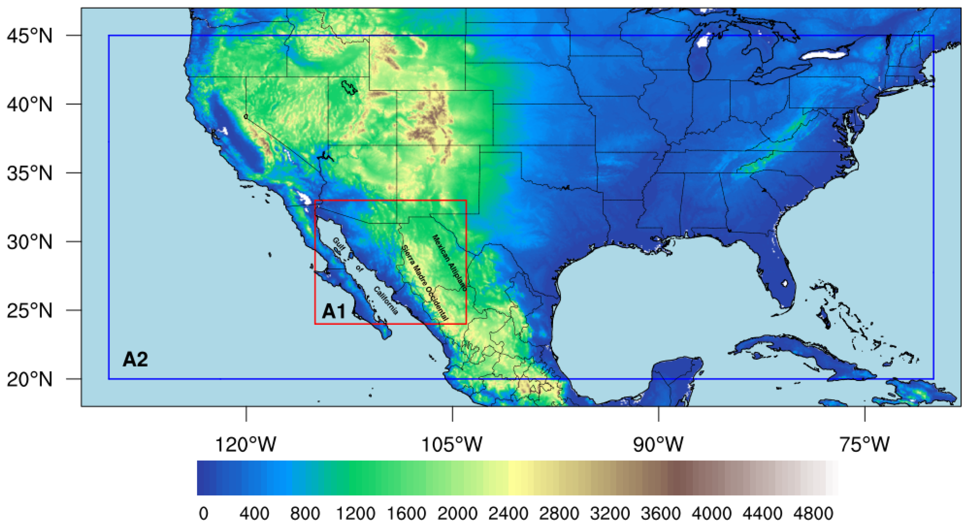
2.1. Study Area

Northwestern Mexico (see Figure 1), provides an interesting natural laboratory to analyze the interactions between topographic features, environmental conditions, the formation and propagation of MCS as well as typical day-to-day convective activity during the NAM. In terms of frequency, most deep convection occurs over the SMO which extends from the Mexican state of Nayarit to the border of Arizona with an average elevation well above 2000 m. In the southern portion of the NAM region, the SMO closely parallels the Eastern Pacific and GoC coasts resulting in a strong sea-breeze circulation and associated low-level moisture transport inland towards the SMO [51,81,82,83]. Northward from Sinaloa, the SMO trends inland and the sea-breeze strength as well as the frequency of deep convective precipitation tend to decrease [81,82,84]. The topographic transition on the eastern slopes of the SMO, unlike the western slopes, is much gentler descending towards the arid Mexican Altiplano of north-central Mexico. Though elevated (∼1500 m), deep convective activity is much less frequent over the northern portion of the Altiplano during the NAM. The SMO western slopes steeply descend, transitioning into a complex basin and range topography, particularly in the northern portion of the study region (e.g., Sonora and Arizona). Approaching the GoC, broad coastal plains with much lower relief dominate. On the opposite coast of the GoC, deep convective activity over the Baja California peninsula tends to diminish presumably due to more frequent incursions of stable, drier air above the Pacific Ocean. The near-complete absence of deep convective activity along the Pacific coast of the Baja Peninsula is reflective of the cooler ocean waters associated with the California Current (see, for example, Figure 5 in Holle and Murphy [85]).

2.2. Data

To begin with, all MCS studies require an MCS definition for identification and classification purposes. This identification process also necessitates proposing a methodology, which must be robust and replicable. In this section, we elaborate on the various data employed in this study for MCS identification and the methodology utilized for tracking their spatial-temporal evolution.

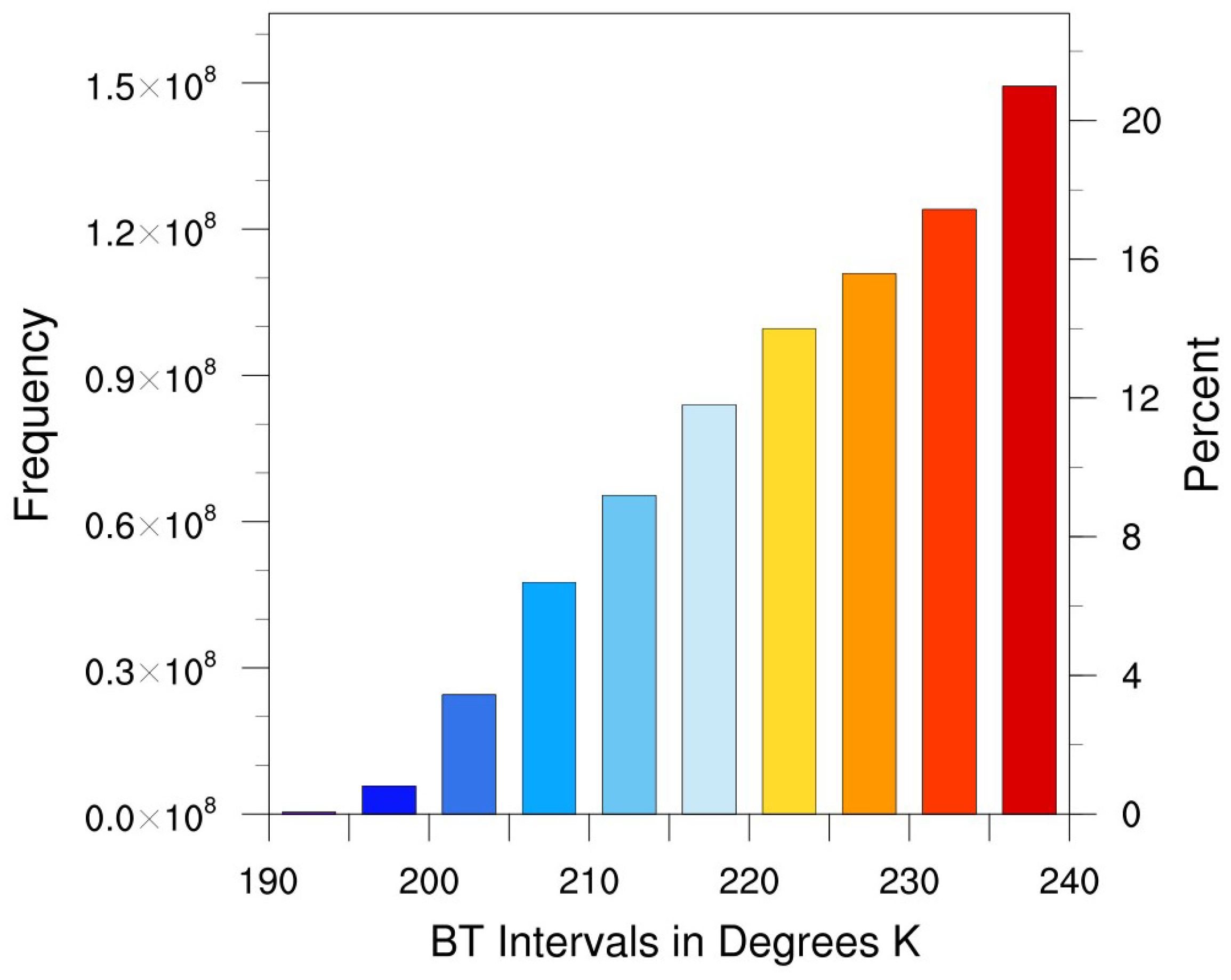
2.2.1. Satellite Images

A large portion of MCS research is based upon satellite imagery, principally, in the thermal infrared bands. These satellite infrared radiance data can be converted into Brightness Temperature (BT), a variable that is closely tied to the evolution of deep convective activity [41,86,87,88,89]. Given that there is often a large contrast between cold cloud tops and the surrounding cloud-free environment, infrared imagery is effective in identifying and monitoring MCS growth and propagation [90,91,92]. Here, we utilize a total of 23 years of GOES IR satellite imagery, specifically the IR band at 10.7 μm for June through September from GOES 8 (1995–2002), GOES 12 (2003–2012), and GOES 13 (2013–2017). GOES IR imagery data have a spatial and temporal resolution of 4 km and typically 15 min, respectively. These GOES Satellite retrievals and information on satellite platforms can be found at https://www.ssec.wisc.edu/datacenter/ (accessed on 14 April 2022).

2.2.2. Lightning

Many studies have demonstrated the utility of long-range terrestrial lightning location systems (LLS) data which employ different sensors operating at Very Low/Low Frequencies (VLFs/LFs) up to Very High Frequencies (VHFs) to provide near real-time lightning data globally [93,94]. Lightning data are particularly useful for identifying deep convective activity being continuous in time and space and, unlike radars, do not suffer from blockage issues in complex topography [85,89,95,96]. Moreover, given the strike location accuracy currently available, lightning data have proven useful in differentiating the convective and stratiform regions of MCS [97,98,99,100]. In this study, we utilize Vaisala’s Global Lightning Detection Network (GLD360) data which provides: location, time of lightning flash, polarity, and peak current estimates. Several studies have evaluated GLD360 performance and shown cloud-to-ground flash detection efficiency of around 60–70% and the median location accuracy at 2–5 km in North America [101]. A more thorough description of the network and data products are found in [102,103]. GLD360 data were employed in previous NAM studies to gauge the spatial and temporal distribution of convective activity Holle and Murphy [85], and to characterize the intensity/evolution of convective diurnal cycle Serra et al. [35]. For this study, we use GLD360 data from 2011 to 2017 as a means for classifying the development and decay of MCS.

2.2.3. ERA5 Reanalysis Data

Studies have shown that reanalysis data are sufficiently accurate in subtropical and tropical regions for gauging propitious synoptic-scale atmospheric conditions for the formation of MCS [70] as well as at higher latitudes [104,105]. ERA5 has a spatial resolution of 0.25° degrees, a vertical resolution of 37 pressure levels, and a temporal resolution of 1 h [106]. Given this high resolution, ERA5 are used to determine synoptic conditions for examining interannual variability of MCS as well as their relationship to propagation characteristics. Specifically, we employ geopotential height, specific humidity, and u and v wind components at 700, 500, and 200 hPa. For specific details on the creation and accuracy of ERA5, see https://confluence.ecmwf.int/display/CKB/ERA5 (accessed on 14 April 2022). Our region of analysis for GOES and GLD360 data is that of Area 1 limited to 24°–33° N and 104°–115° W (see Figure 1) which roughly corresponds to the NAME Tier 1 area [64], however, not extending as far south. Area 2 corresponds to the synoptic-scale analysis utilizing ERA5 data, consistent with the studies of [66,80], which examine NAM area convective activity in a nested modeling context.

2.3. GOES IR Classification of MCS

One of the pioneering works in the MCS classification employing geostationary infrared satellite images is the study of Maddox [44]. He defined a circular shaped MCS as an MCC according to certain characteristics in its shape, area, and duration (see Table 1 in [44]) for MCS in the central United States. Further studies from various regions around the globe have also found these circular systems to be common [107,108]. Augustine and Howard [109] proposed that the BT threshold of 221 K adequately represented the full development of an MCC; a criterion that has also been utilized in other studies [40,110,111,112]. Anderson and Arritt [45] define another type of MCS, which meets the size and duration criteria put forward by Maddox [44], but not with the same form, which they denominate PECS, as described above. However, Jirak et al. [40] found that these criteria and thresholds can occur on even smaller scales which they define as Meso-β Circular Convective System (MβCCS) and the Meso-β Elongated Convective System (MβECs) (see Table 1 in Jirak et al. [40]).
These morphological definitions are for the most part derived from relatively flat, mid-latitude regions; for example, the Great Plains in the central United States. There is, in fact, no universal BT criterion nor areal extent for defining an MCS, though, these criteria are not entirely arbitrary. BT criterion values have varied from 208 to 245 K, while the minimum threshold for the area has ranged from 1000 to 100,000 km2 [59,86,88,113,114,115,116,117]. Taking this variation in criteria into account, in this study, a histogram of BT values was created (Figure 2) considering pixels falling into the range of BT values (208–245 K) for the 23 summers of the study. From this histogram, the mean temperature 220 K is taken as an appropriate value for the NAM region. Furthermore, 220 K is similar to values utilized in other shorter-term studies of MCS, such as Valdés-Manzanilla and Barradas Miranda [62] and Mejia et al. [63]. Here, a minimum value of area corresponding to 5000 km2 was imposed, a value frequently used in MCS studies in tropical and subtropical regions [88,92,113,117,118].
In terms of MCS temporal evolution, the initiation time is defined as when a system meets the following criteria: area (≥5000 km2) and BT (≤220 K). MCS dissipation is designated as the point in the temporal evolution when these criteria are no longer met. Similar to Farfán and Zehnder [59], we only analyze MCS that have a duration of minimally 6 h, hence focusing are longer-lived events. Similar MCS lifetimes have also been utilized in tropical and mid-latitude regions [44]. With these above criteria, 1594 MCS were identified in Northwest Mexico from 1995 to 2017 during the monsoon season from June through September. Once identified, MCS were then classified in terms of cirrus shield excentricity. An MCS is considered circular and elongated when its eccentricity ( ϵ ) is greater than or less than 0.7, respectively (Figure 3). As in previous studies, we classify these MCS, as MCC ( ϵ > 0.7) and PECSs ( ϵ < 0.7) [40,41,45,119].

2.4. MCS Detection Algorithm

MCS identification and monitoring still remain a challenge given that cloud growth and cirrus shield areal expansion can vary relatively quickly. Further complicating their identification, they can split resulting in two or more MCS, or join together with other MCS [86,88]. After identification based on the above-mentioned criteria, the trajectory of each MCS is determined by following its cirrus shield for successive satellite images [113,120,121]. Two methodologies that have proven useful for determining MCS trajectories are the area overlap method (AOL) [113] and the method of maximum spatial correlation [121]. The AOL method is based on the consideration that an MCS, in successive frames, represents the same system if their pixels overlap from the current to the following timestep, for at least 15 to 50% of the pixels or 500 to 5000 km2 of pixel area [86,113,122,123]. This method has been applied to various regions of the world, for the Amazon region [116], in the La Plata basin [124], in the Sahel [86]. More recently, Huang et al. [88] developed an algorithm based on AOL for tracking MCS in tropical and subtropical regions on a global scale. The maximum spatial correlation method takes into account the relationship between the MCS cloud shield radius and the BT threshold which have a correlation threshold of 0.3 for systems in successive images, thereby representing the same MCS. As such, MCS in relatively close proximity with little change in the horizontal area between consecutive images are considered to be the same system. This technique has been used to track MCS in South America [121], Spain [125], southern Africa [112] and recently in China [41].
In the present study, the AOL methodology was chosen because it offers better tracking and greater certainty compared to maximum spatial correlation, since AOL is not affected by the distance the MCS travels in consecutive images compared to maximum spatial correlation. In the latter method, the calculation of the Euclidean distance is made either from the MCS’s center of gravity or from the center of the ellipse and is affected by merging and splitting processes [124]. We speculate that for the NAM region with its complex terrain, processes of merging and splitting should occur with greater frequency during the MCS life cycle. In agreement with previous studies, we employ an overlap of 25% [92,113,116,122,124,126]. The following criteria are utilized in this study: (1) MCS which during their life cycle neither merge nor split, (2) MCS that during their life cycle merge with other systems resulting in an areal extent of at least 5000 km2, (3) MCS which during their life cycle split into two or more systems of at least 5000 km2; the system with the greater area is tracked. Finally, MCS that result from the union of different systems remain smaller than 5000 km2 are excluded in order to analyze MCS with a more clearly defined life cycle [127].

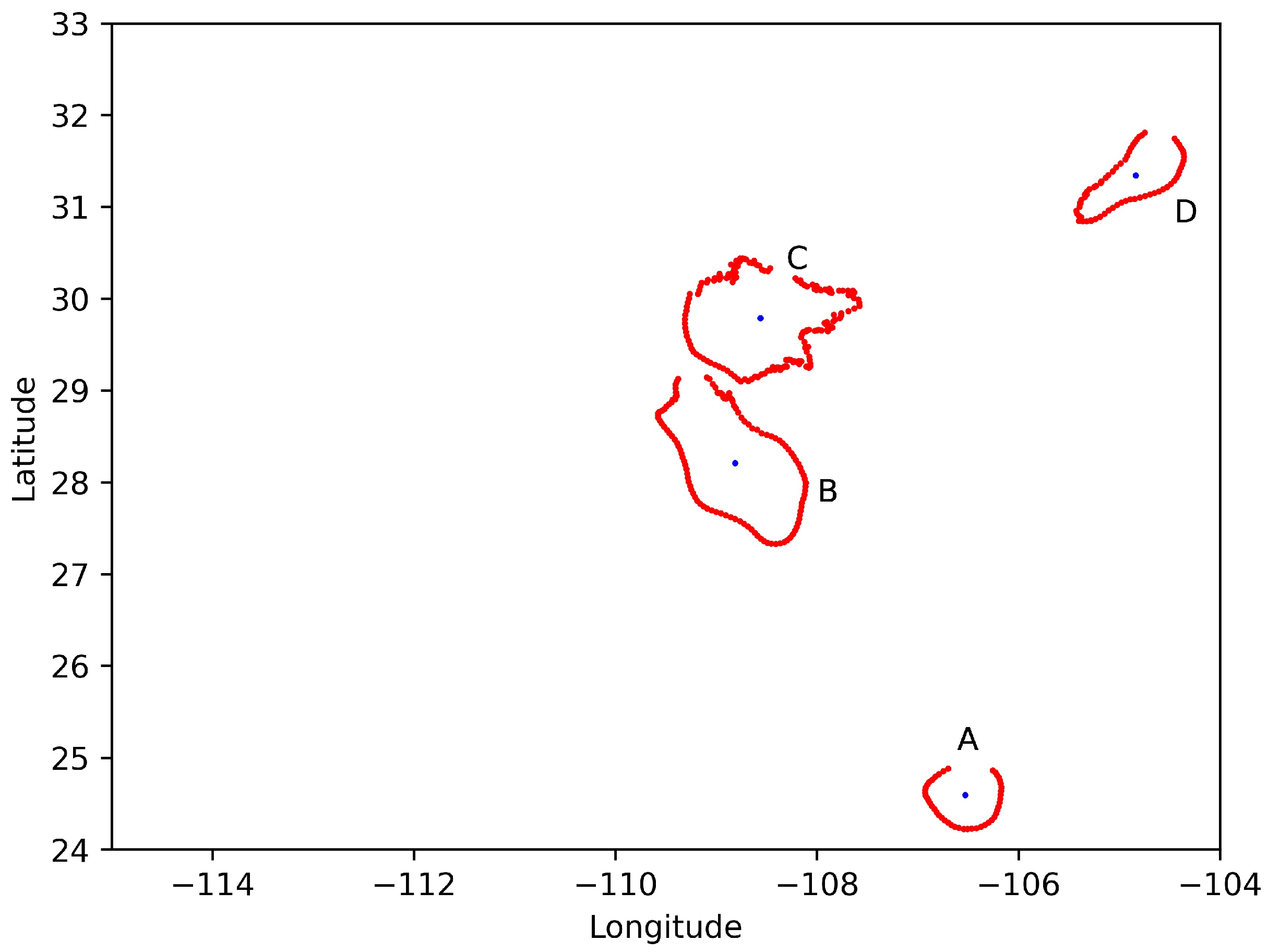
2.5. MCS Trajectory Analysis

Given the large number of MCS occurrence, we simplify NAM MCS trajectory analysis, by creating three, 3-degree latitudinal bands. Figure 4 contains the initiation location for MCS for these three different latitudinal bands utilized: 24°–27° N, 27°–30° N and 30°–33° N called Band A, B and C, respectively. Within each one of these bands and for those MCS propagating parallel to the SMO (e.g., crossing latitudinal bands), propagation velocity is estimated by way of Hovmöller diagrams in addition to simply calculating the velocity based on the initial and final position of the MCS centroid. For the purpose of analyzing MCS trajectory at the more extreme ends of interannual variability, we create composites of synoptic conditions for the 2 most active and the 2 least active years in terms of MCS occurrence. Selecting these extreme years provides a measure of the bounds that we may expect on MCS behavior. Likewise, with respect to monthly variability during the evolution of the monsoon, initial and final point of MCS trajectory are plotted for a visual representation of typical paths for each month, June through September.

3. Results

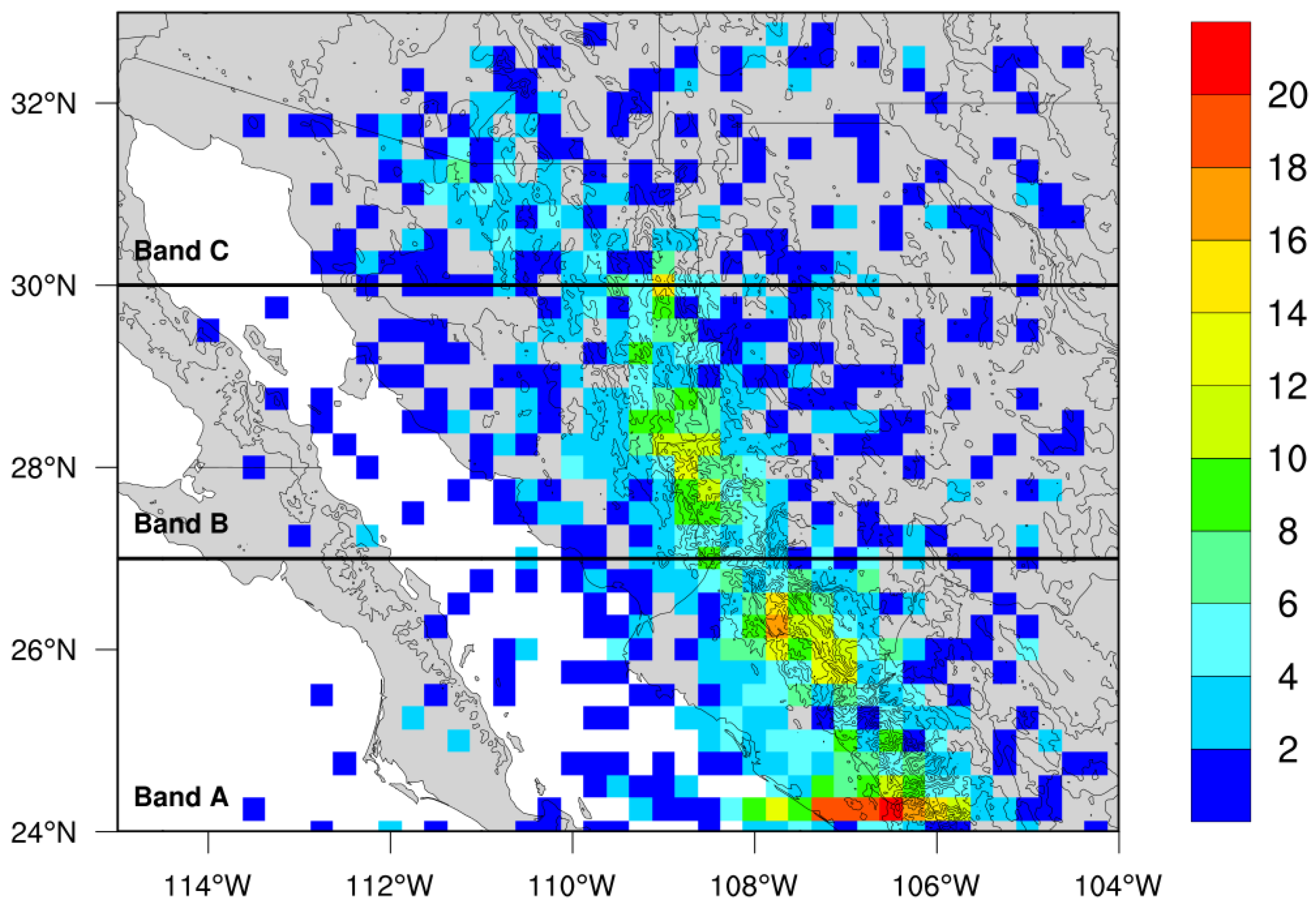
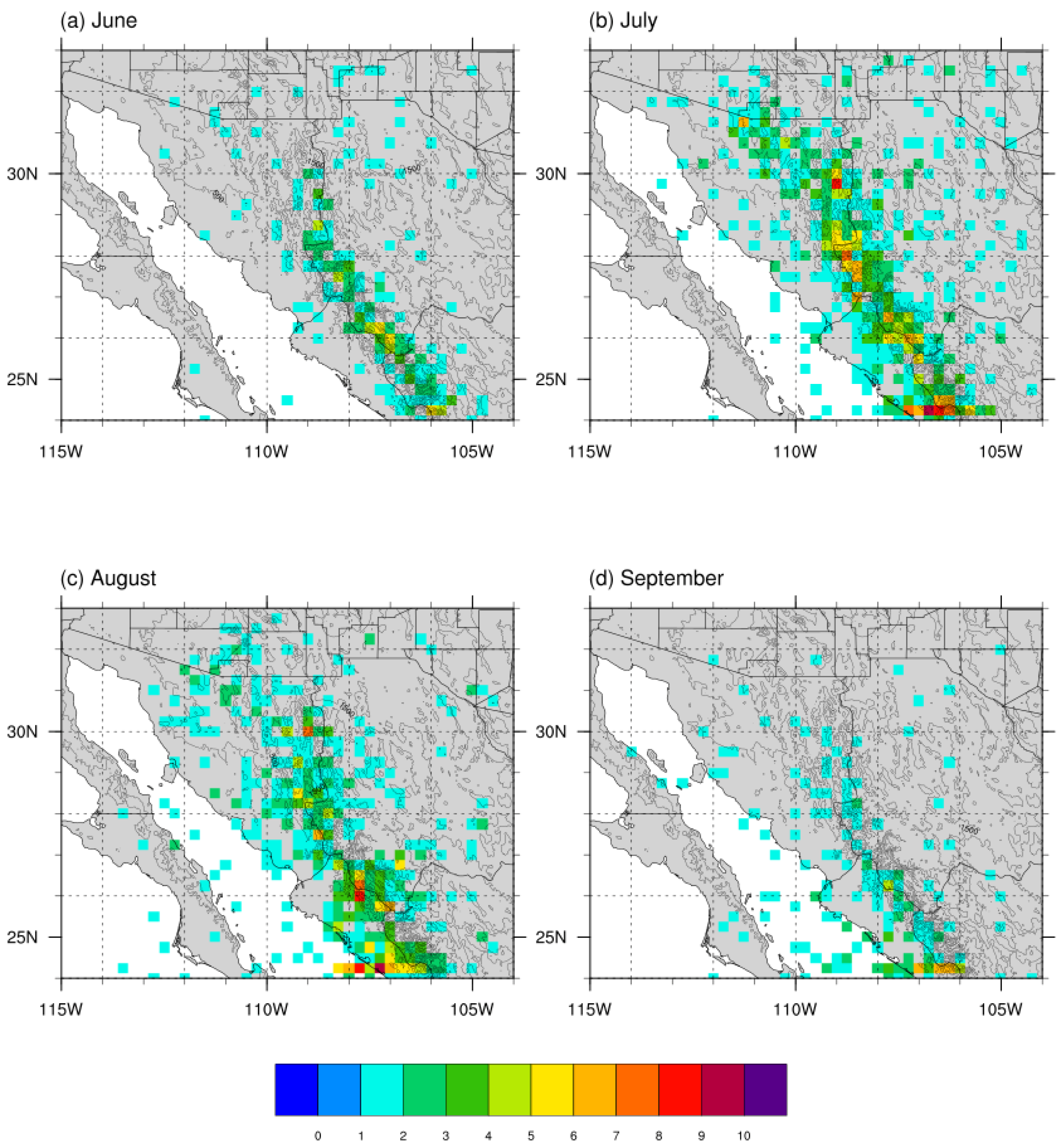
3.1. Spatial Distribution

During the 23 summers from 1995 to 2017, 1594 MCS were identified in northwestern Mexico. In Figure 4, the spatial distribution of MCS initialization is plotted. Not unexpectedly, the number of MCS events is largest along the southern coastal plains of Sinaloa and along the western slopes of the SMO. The number of MCS tends to decrease northward into the state of Sonora. Likewise, MCS tend to be much less frequent on the eastern slopes of the SMO and the Mexican Altiplano. Within Band A, nocturnal MCS are frequent, particularly along the western slopes of the SMO [56,70,85]. In band B, the majority of the MCS initiate near the crest of the SMO. Within B and C, perhaps not surprisingly given results from previous studies, there are relatively fewer MCS with very dispersed points of initiation. The convective development in the Bands A and B are probably most closely tied to low-level, upslope flow from the GoC [52] and resulting abundance of water vapor [56,68,69], although dynamical mechanisms such as increased shear have also been argued to be critical for MCS formation and propagation. In band C, the influence of the position of the subtropical anticyclone, migrating southward, fewer incursions of IVs, as well as intrusions of drier air from the northwest, result in diminished occurrence of MCS and convective activity, in general [78,85,128].
With respect to MCS morphology, the vast majority of the MCS, approximately 98%, belong to the PECS category while only approximately 2%, were characterized as MCC. Therefore, in this region characterized by its complex orography, PECS which also typically initiate of the SMO entirely dominate the morphology classification. This PECS domination associated with the complex terrain and with the orographic uplift is similar to what occurs in the mountain ranges of central Europe (e.g., the Pyrenees and the Alps) [129,130] and the Himalayas [41]. These results are also consistent with those of Jirak et al. [40], who found that in the relatively flat topography of the central Plains MCC and PECS have similar frequency, supporting the argument that complex topography strongly impacts MCS morphology. In addition to their minuscule frequency of occurrence, MCC are quite scattered in terms of their location of origin, including the northern region of the NAM near the United States border (e.g., Sonora-Arizona, Chihuahua-Texas) and both east and west of the SMO.

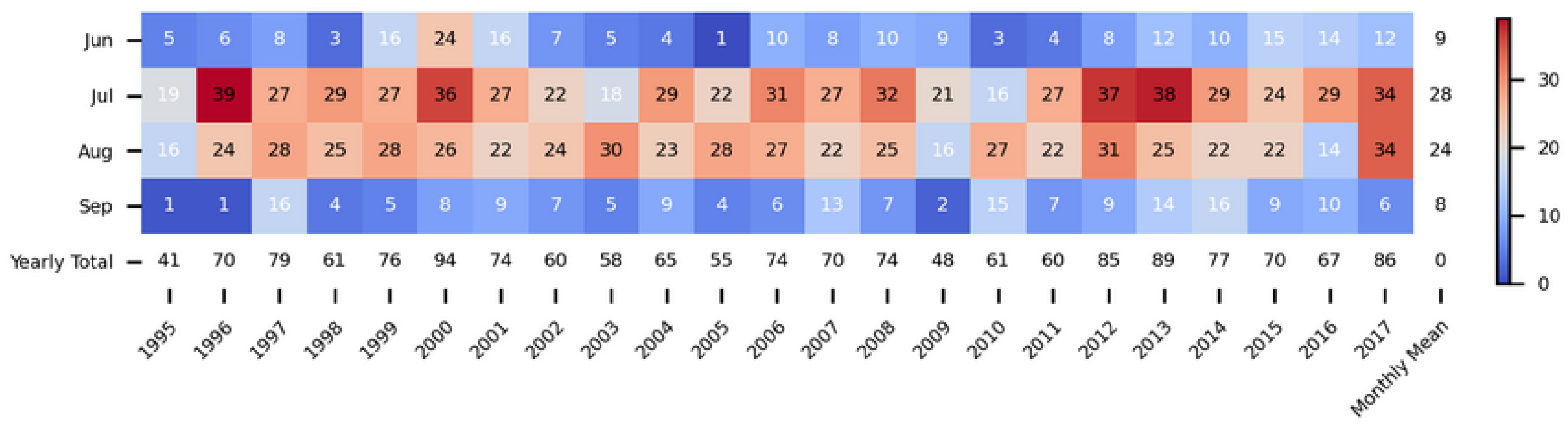
3.2. Interannual and Monthly Variability

Although the NAM occurs every summer, it experiences interannual and inter-seasonal variability in terms of the frequency of convective activity [48,131,132,133]. During the 23 summers observed, the number of MCS varied considerably, with an average of 70 systems per summer and ranging in number from 41 to 94 MCS. In Figure 5, the interannual as well as monthly variability is presented in the form of a heat map. With ERA5 geopotential, specific humidity, and winds at 500 hPa, in order to frame the boundaries on MCS occurrence, composites were made for the 2 most active years (94 events in 2000 and 91 in 2013) and the two least active years (41 events in 1995 and 53 events in 2009). We found that for the two most active years, the subtropical high was displaced relatively farther north and more intense compared to the least active 2 years. This northward migration and intensification of the monsoon ridge may allow for penetration of lower-level moisture into the southwestern U.S. with attendant decreases in atmospheric stability as well as the passage of transient disturbances which increase vertical wind shear profiles, such as IVs [57,71,134,135]. In the case of IVs Douglas and Englehart [136] found that IVs are the most common transient synoptic factor though the actual mechanism for intensification and occurrence of MCS due to IVs has been debated [54,77].
As with other monsoonal regimes such as Australia [137], Africa [138], and Asia [139], NAM variability in synoptic flow pattern is large and is fundamental to the outbreak or suppression of deep convective activity. Widespread convective activity associated with burst and break periods typically lasts on the timescale of weeks [48,74,140,141]. Intense convective activity and associated MCS occur during burst periods and typically depend on synoptic or subsynoptic disturbances with timescales of several days to a week [78,135]. Figure 6 contains the spatial distribution of the locations of MCS initialization from June to September. The month-to-month variations that can be observed are an increase in the number of organized systems and the geographical region where MCS tend to occur with greater frequency. In June (Figure 6a), there is a very active zone of MCS initialization along the SMO corridor. There are also MCS that initiate far removed from the SMO corridor, for example, along the Baja California peninsula as well as over the Mexican Altiplano, though much less frequently. During the months of July and August, where conditions are hot and humid over a much larger region (Figure 6b,c, respectively), the NAM circulation is well established and there is a notable increase in MCS occurrence along the SMO and along the coastal region of Sinaloa. Approaching the end of the NAM (September, Figure 6d), there is a strong decrease in MCS initiation along with the SMO corridor, though the coastal region of Sinaloa remains relatively active.
Regarding monthly variability, as expected, the most active months are July and August where conditions are generally more humid and less frequent intrusions of drier westerly winds compared with June and September [47,48,142]. However, in this longer climatological study, we found that for several years (1999, 2000, 2001, 2015, 2016), June was essentially as active as the more typical peak monsoon months of July and August. Likewise, for the years 1997, 2010, 2013, and 2014, September was quite active in terms of MCS occurrence. As mentioned above this variability in MCS has been tied to the occurrence of IVs. In a future study, we will examine possible synoptic conditions that are associated hiked occurrence of MCS in normally more quiescent months.

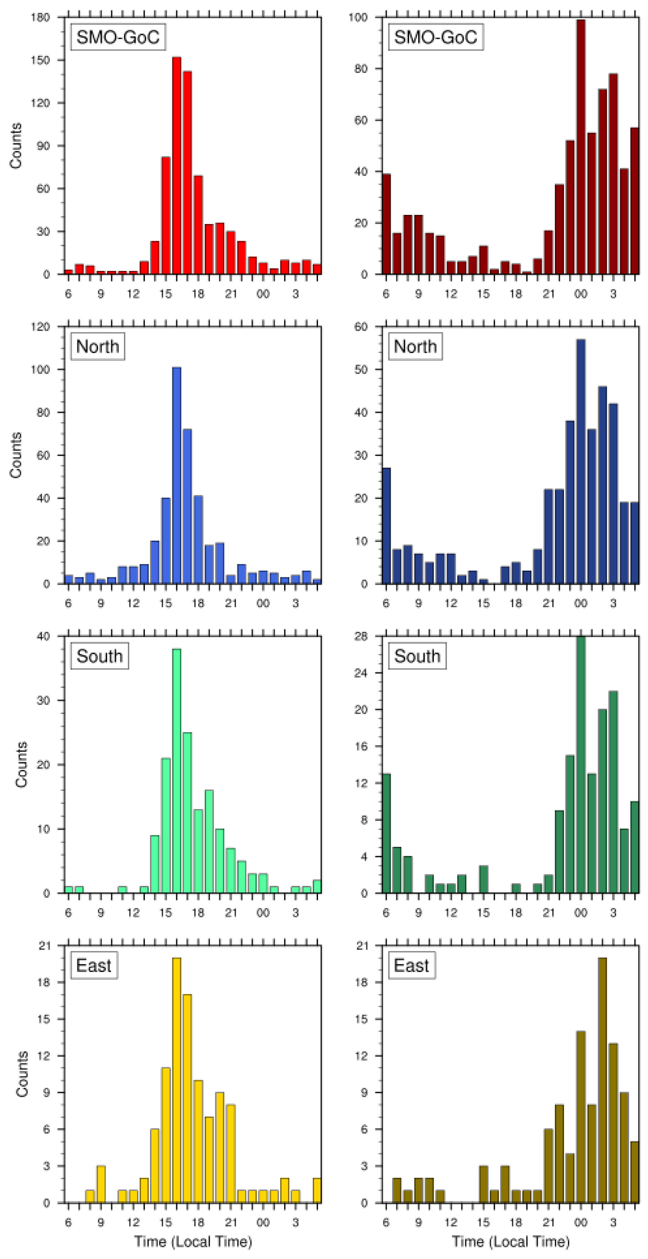
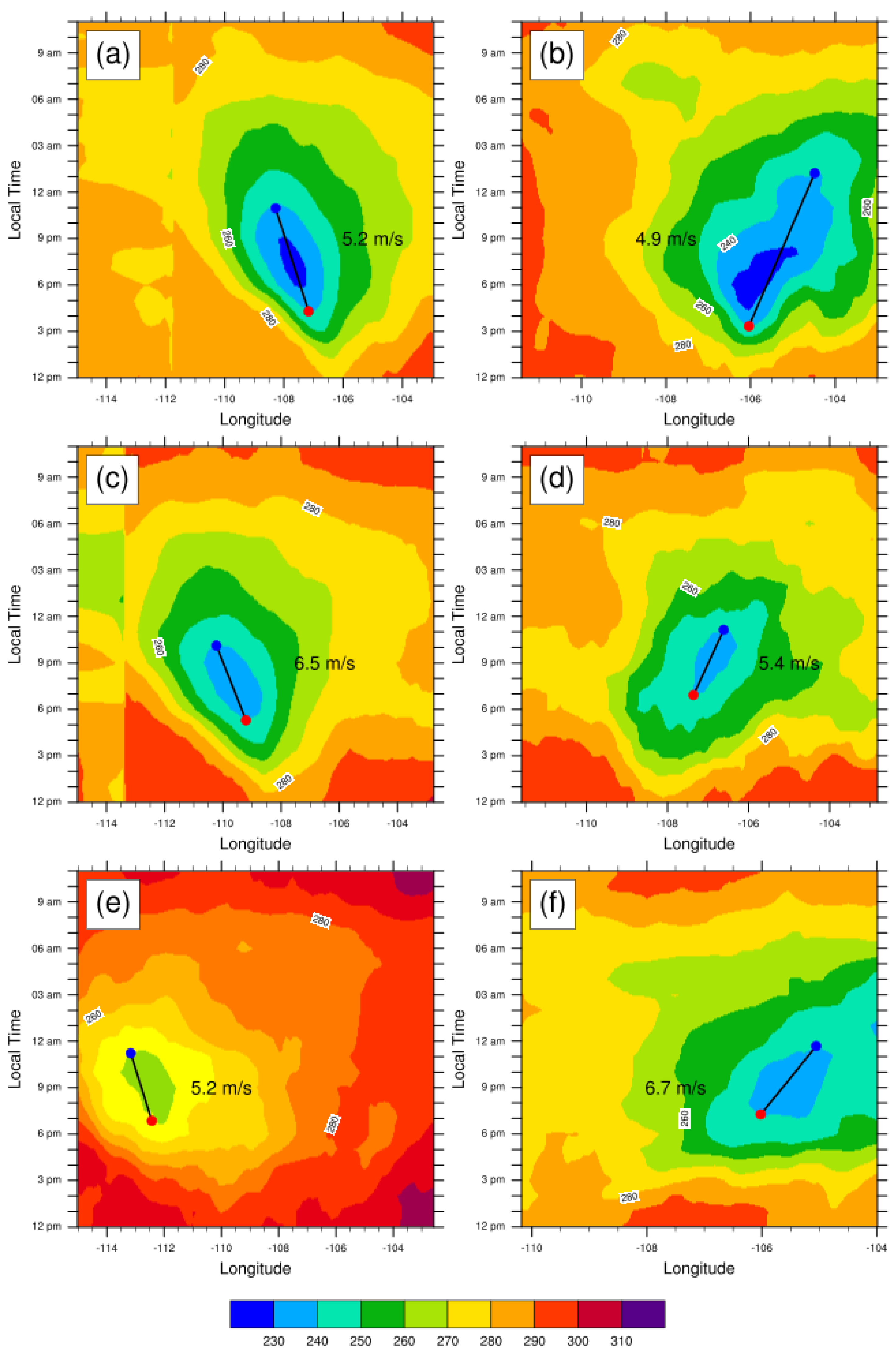
3.3. Diurnal Cycle of MCS

Figure 7 shows the diurnal cycle for two important stages in the life cycle of MCS: initiation and dissipation. While it is true that MCS can commence, grow and dissipate at any time of day, it is important to verify if these stages are strickly linked to diurnal variation of solar radiation as has been noted in other regions of the world [40,41,111,112]. The northerly directed MCS, (Figure 7 middle panel) have a narrower time range of initiation (13:00–20:00 Local Time (LT) (UTC-6)) compared with the other trajectories (14:00–02:00 LT), which indicates that favorable atmospheric conditions for these northerly directed MCS initiation are more constrained. However, independent of trajectory, MCS occur predominantly between 14:00 to 21:00 LT, the time which coincides with intense precipitation events mainly along the western slopes of the SMO [67,69]. This temporal range also coincides with that reported by Valdés-Manzanilla and Barradas Miranda [62], who found that in the summer of 2004, 77% of MCS usually start between 15:00–21:00 LT. In our climatological study, the initiation of MCS increases notably after midday, reaching a maximum value at 16:00–17:00 LT. Nesbitt et al. [69] argued that deep convection typically commences around noon along the highest ridges of the SMO and, similar to our results, the mesoscale organization typically occurs after 15:00 LT when conditions are most favorable in terms of sufficient moisture and thus convective available potential energy (CAPE).
The time 16:00 LT was observed to be the most frequent time of MCS occurrence for MCS perpendicular (Figure 7 upper and bottom panel) and parallel to the SMO (Figure 7 middle panel). On the other hand, we found that 00:00 LT is the most common time of MCS termination which is observed in the Figure 7 right column, except for MCS traveling from SMO eastward towards Chihuahua (02:00 LT). However, independent of trajectory, MCS dissipation occurs between 00:00 to 09:00 LT, a result similar to that reported by Valdés-Manzanilla and Barradas Miranda [62] during the summer of 2004. In contrast to Valdés-Manzanilla and Barradas Miranda [62], our long-term analysis indicates that MCS do dissipate between (18:00–21:00 LT), perhaps due to the lack of a forcing mechanism which enhances MCS organization, propagation, and overall lifetime. With respect to MCS lifetime, our longer term results indicate that MCS typically have an average duration of around 8 h ± with a 2 h standard deviation, a minimum of 6 h (the minimum time criterion employed in this study), and a maximum of 27.50 h.

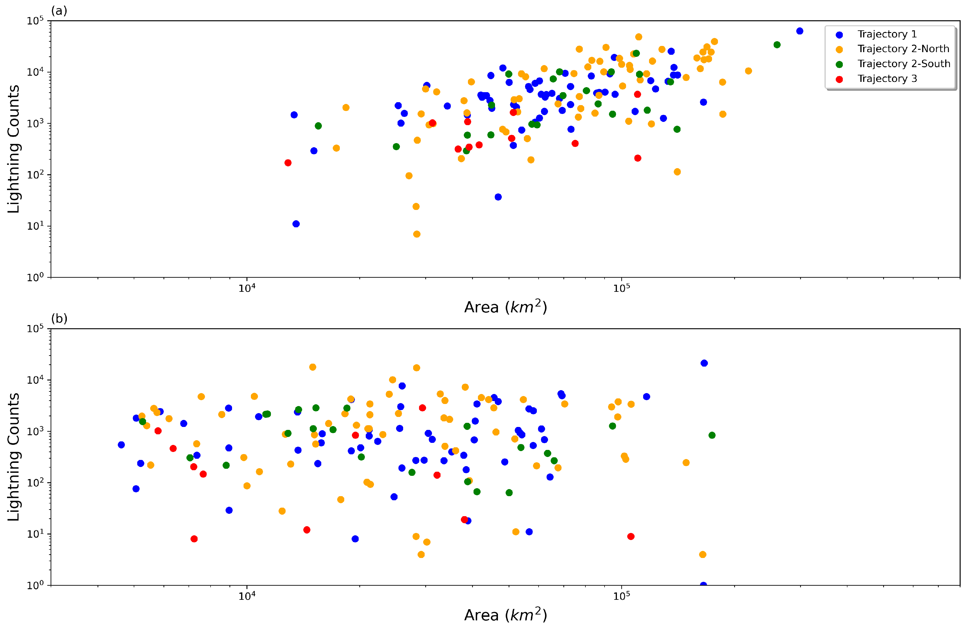
3.4. Lightning Activity of MCS

The increase in lightning activity during the development stage of MCS is a response to the rapid updraft intensification, that is, a strong updraft would lead to an increase in ice particle collisions which increases the separation of charge and with it an increase in lightning occurrence [143,144,145,146]. Although, lightning is typically categorized into three groups, intra-cloud, cloud-to-cloud and cloud-to-ground [146,147,148]; cloud-to-ground, in particular, has been employed in MCS studies [100,149,150,151,152,153]. Approximately 80% of GLD360 detection strokes are estimated to be cloud-to-ground [85]. The lightning activity of the MCS meeting the criteria of our study (see Section 2.3) are analyzed only for the summers of 2011–2017 given data limitations. This is evaluated considering two stages in the life cycle of MCS: Stage 1 (Start-Maturity) and Stage 2 (Maturity-Dissipation).
Figure 8 shows the summation of lightning strikes (y-axis) during the two stages versus the area of the MCS (maximum and final area represent the value of x-axis in upper and bottom panel, respectively) for all MCS Trajectories. Regardless of the trajectory, we found a greater number of flashes during stage 1 (Figure 8a) when compared to stage 2 (Figure 8b), which is consistent with convective development when updrafts tend to intensify in the convective region of the MCS [1,2,13]. However, the MCS of trajectory 3 are relatively less intense with fewer lightning flashes in comparison with the other trajectories. This decrease in lightning occurrence may be likely the result of a diminution in the number of thunderstorm hours, which are defined by [85] as any hour of UTC time in which one or more lightning strokes is observed within a 40 km by 40 km box. However, the enhanced lightning occurrence, in all trajectories, may be due to the strengthing of convective updrafts by the upslope terrain of the SMO as has been encountered in other regions [101,154,155,156]. In addition, we found a positive trend, more well-defined especially during stage 1, in the lightning versus area relationship; that is, as the MCS become larger, a greater lightning occurrence is observed. This relationship was also found in previous studies. For example, Mattos and Machado [100] found a rapid linear growth in the area is associated with a strong increase in the electrical activity of MCS in Brazil and Makowski et al. [157] found MCS with higher maximum total flash rates tended to be associated with larger cloud shields (shown for the −52 °C cloud shield) in Oklahoma.

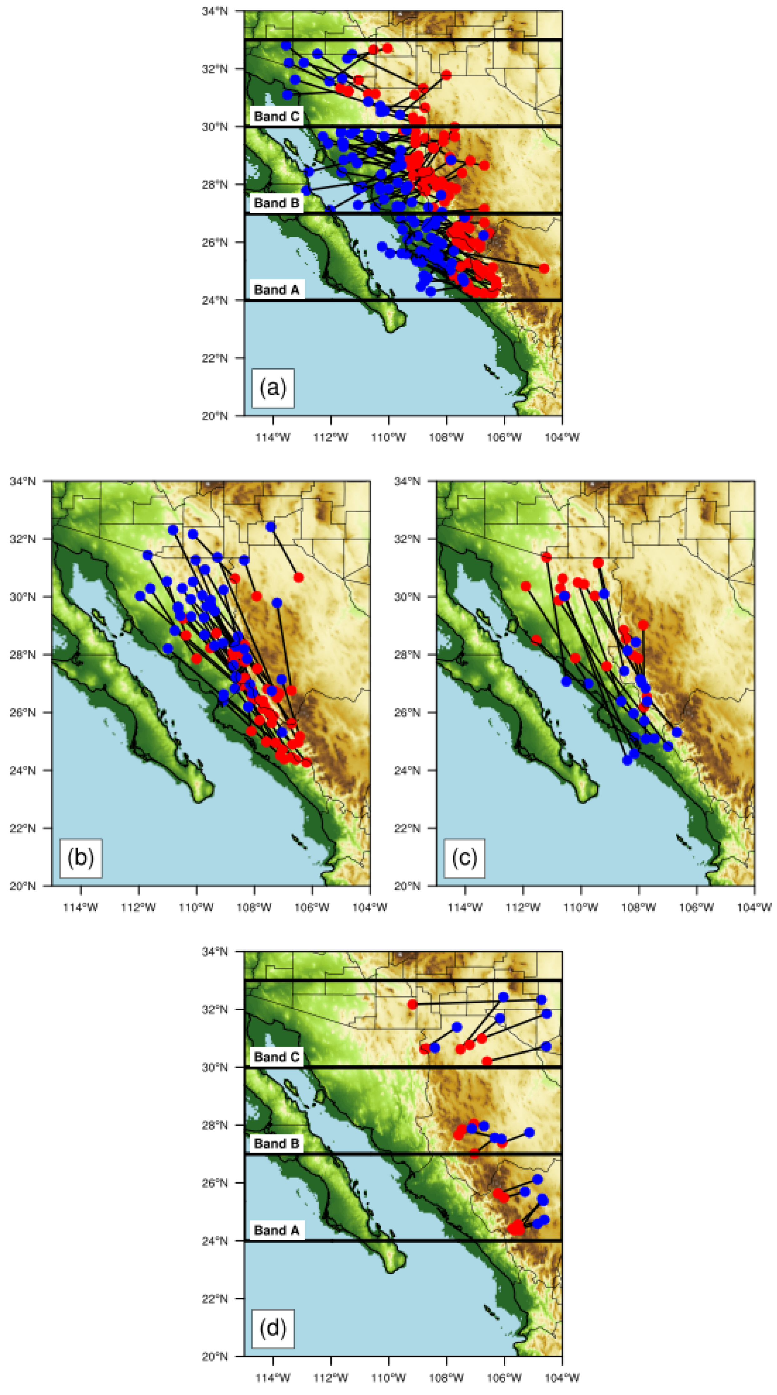
3.5. MCS Propagation

Once MCS have been initiated, they may either remain quasi-stationary or propagate at a given speed. For example, Farfán and Zehnder [59] showed typical displacements of 100 km in 6 h. MCS propagation may be either continuous or discrete. The first case occurs when the MCS progresses toward initiating nearby deep convection is starting and joins with it. In the second case, a new convective system develops relatively distant from the already existing MCS, e.g., ∼30 km [1,158]. The actual mechanism responsible for the propagation of MCS such as cold pools, density currents, and/or gravity waves is still widely debated [159,160,161,162]. Houze [1] and Fovell et al. [158] suggest that continuous propagation was due to the persistence of cold pool dynamics. These ideas have been considered by other authors (e.g., [163,164]). In others studies, it has been argued that gravity waves dynamics may be responsible for MCS discrete propagation [21,28,165,166]. With respect to MCS trajectory, our results suggest three types of trajectories: Trajectory 1 (MCS which progress towards the GoC from the SMO), Trajectory 2 (MCS which travel parallel to the SMO), and Trajectory 3 (MCS traveling from the SMO toward Chihuahua) with 44%, 35%, and 14%, respectively. The trajectories 1 and 2 are similar to Regime A and Regime B as identified by Lang et al. [56] during the NAME campaign of 2004. In addition, they both occur in the zone between the SMO and the GoC coast. This same region has been shown to experience the most intense convective rainfall and lightning stroke density [67,84,85].
Investigating the propagation velocity of MCS is not only of fundamental scientific interest, but is also of utility for operational severe weather forecasting given that estimating approximate time-of-arrival is important for early warnings and severe-weather preparedness [167,168]. In addition, for a region of complex terrain such as the NAM, exploring which mechanisms are responsible for MCS propagation is an urgent task [23,159,161,169,170]. For the purpose of this study, we focus on MCS occurring between 2011–2017 so that lightning data can be employed to explore the intensity and convective lifecycle along these three common trajectories. As before, these MCS must have a lifespan of minimally ≥6 h and initiate between 14:00–22:00 LT. Figure 9 contains trajectories, based on their point of initiation and dissipation, for these MCS.
The MCS propagation speed, for the trajectory types 1, 2, and 3 was estimated by way of two techniques: (1) Hovmöller Diagrams and, (2) the change in centroid position from initial to final lifecycle stage. Both procedures show similar MCSs propagation speed values for Trajectories 1 and 3. Figure 10 shows propagation speed values for the Trajectory 1 (left panel a, c and e) and Trajectory 3 (right panel b, d, and f). While, the speeds for trajectory 1 in bold and 3 in italic are seen in Table 1, Table 2 and Table 3. The values for Trajectory 1 estimates, by the Hovmöller and the change in centroid position in parenthesis, are 5.2 m/s (6.17 ± 3.01 m/s), 6.5 m/s (7.01 ± 3.01 m/s) and 5.2 m/s (7.13 ± 2.64 m/s) for the Band A, B, and C, respectively. For Trajectory 3 are of 4.9 m/s (4.08 ± 1.02 m/s), 5.4 m/s (3.52 ± 1.55 m/s), and 6.7 m/s (6.41 ± 3.79 m/s) for the Band A, B, and C, respectively.
The change in centroid position estimate a velocity for MCS, for Trajectory 2, propagating northward or southward of 8.71 ± 2.68 m/s (Table 4) and 9.42 ± 5.11 m/s (Table 5), respectively. However, the Hovmöller technique has problems in this trajectory likely because MCS have very different speeds and directions of propagation and, when averaged, the averaged trajectory is not representative. In addition, it is important to mention that the propagation speed detection limit is 4 km/15 min ∼4.4 m/s due to the temporal and spatial resolution of the GOES data.
These results suggest that MCS trajectory 2 propagate relatively more quickly than those trajectory 1. These results are consistent with those of Lang et al. [56] from the NAME campaign. These propagation speeds are much less than those associated with gravity waves (≈15 m/s) as discussed by Mapes et al. [28] and relatively larger than advection speeds associated with “steering-level winds” between 700 and 500 mb from ERA5, where the observed ranges were 5.3–6.0 m/s and 3.3–4.6 m/s for MCS trajectory 1 and MCS trajectory 2, respectively). These velocities are more consistent with propagation associated with density currents or cold pools resulting from MCS downdrafts. A similar mechanism was proposed by Lang et al. [56] and Rowe et al. [61] given the observed MCS propagations speeds during NAME. Nevertheless, the lack of long-term, high spatial density surface meteorological networks impedes the verification of this proposed mechanism.
Previous studies have demonstrated that synoptic-scale conditions can influence certain characteristics of MCS including their initiation, duration, morphology, size, and propagation speed [139,162,171,172,173]. With respect to the NAM, studies have also shown that synoptic flow can create favorable conditions for MCS development [63,70,71,135,140,141,174]. In Figure 11 and Figure 12 composites of geopotential, winds, and specific humidity in different atmospheric levels (700, 500, and 200 mb) during convective initiation are shown for MCS which propagate towards and parallel to the GoC, respectively. From the figures, it is apparent that the winds are fairly weak and the geopotential height is displaced northward in congruence with the northward progression of the latitudinal band. A similar northward extension in the humidity fields is also observed. In particular, trajectory 2 MCS typically occur in moister environments compared to trajectory 1 indicating the role of atmospheric instability in moisture environments [17,18,22].

4. Summary and Discussion

The Northwest region of Mexico experiences an increase in convective activity every summer, which tends to produce significant amounts of rain in this semi-arid and arid region with complex orography. Several field campaigns have been carried out in the last few decades in order to understand the formation, spread, and other aspects of convection organization in MCS [64,175]. Through the use of satellite images and lightning, this study is an attempt to gain insight into MCS including their temporal and spatial distribution, their morphology, and their intensification. Using an identification algorithm and a semi-automatic follow-up method, 1594 MCS were identified over the study region during the summers of 1995–2017.
Table 6 summarizes the MCS characteristics with respect to their morphology and trajectory. In general, PECS, on average, last longer, propagate greater distances with greater velocity and display a larger initial area when compared with MCC, similar to what has been reported in other studies [40,41]. However, all MCS within the NAM region, independent of their form (PECS and MCC) and their trajectory (1, 2 and 3), have less eccentricity and shorter lifespan compared to MCS reported in the central U.S. perhaps as a function of the topography ([40]) and the Himalayas region ([41]) maybe a result of weaker NAM region sinoptic forcing.
Regarding their spatial distribution, three latitudinal bands were identified where MCS tend to start with greater frequency. Bands A and B which experience the strongest precipitation events during the monsoonal season resulting from the occurrence and spread of MCS [56,67,68,69]. It was also observed that the activity tends to be lower in the northern portion of the study area, Band C, most likely due to less frequent moisture incursion [176,177], as well as the lower occurrence of forcing of synoptic scales (e.g., IVs; [78], and a weakening of a diurnal sea breeze circulation [51]. While on the east side of the SMO the little occurrence of MCS are probably the result of weaker convergence, the lack of moisture in the atmospheric column relative to the western slope of the SMO [51,52].
The summers of 2000 and 2013 were the two most active summers with 94 and 91 MCS, respectively, while 1995 and 2009 were the two least active summers in terms of MCS, 41 and 53, respectively. For the two most active years, the subtropical high was displaced relatively farther north and more intense compared to the least active 2 years (Figure 13), which also favors the passage of transitory disturbances (e.g., IVs) which can provide a favorable wind shear profile for the formation and propagation of MCS [53,54]. The monthly frequency shows that the most active month is July, followed by August. While June and September were the least active, confirming what would be expected, since the NAM usually starts in mid-late June, its maturity is observed in July and August, while its dissipation occurs in mid-late September [142].
MCS in this region have an average life of 8.28 h relatively higher than that found (7.46 h) in the summer of 2004 by [62]. It is important to mention that our study covers 23 summers and therefore the discrepancy with [62] is probably explained by the interannual variability in synoptic conditions that favor the development and maintenance of these organized systems [78,134,136]. The maximum duration was 27.50 h, the minimum of 6 h (given by the definition of MCS used in this study). With regards to their morphology, most of the MCS have an eccentricity of less than 0.7, which indicates that these systems tend to have an elongated shape. Considering the diurnal cycle of MCS, approximately 75% usually start during the afternoon and early evening (14:00–20:00 LT); while 50% tend to dissipate in the early morning (20:00–04:00 LT) similar to that reported by [62] and similar to the diurnal cycle of convective activity and precipitation, where MCS start during the afternoon mainly on the western slopes of the SMO and are capable of generating heavy rain in these areas and even in coastal regions while heading towards the GoC [56,67,68,69].
For this study region, our evaluation of lightning activity with respect to two stages in the life cycle of MCS; Stage 1 (Start-Maturity) and Stage 2 (Maturity-Dissipation), we find that these systems usually have greater lightning occurrence during the Stage 1 similar to what has been reported in both mid-latitudes and certain tropical regions [100,152]. In previous studies employing radar, the strongest updrafts have been seen during the initiation stages [1,2,13].
With respect to MCS trajectory, the results from our long-term climatology using GOES IR data suggest two dominant trajectories: Trajectory 1 (MCS which progress towards the GoC from the SMO) and Trajectory 2 (MCS which travel parallel to the SMO) with 44% and 35%, respectively. In both trajectories, the favorable 500 mb geopotential height pattern is similar, with a broad anticyclonic circulation centered over New Mexico. This positioning of the monsoon ridge to north and east and can provide a favorable environment (e.g., suficient amounts of moisture in the boundary layer, atmospheric instability, vertical wind shear and lifting mechanism that triggers convection) for MCS [71,140,178]. This synoptic pattern corresponds to the type I severe weather pattern previously identified by [71], and first and third mode of empirical orthogonal function analysis by [57,174], respectively. Our examination of propagation speeds suggest that cold pools or density currents and not gravity waves nor mid-level winds are responsible for the propagation of NAM MCS, however, more surface sites are needed to validate this observation. Previous studies have identified two main mechanisms that can explain the MCS motion: (1) Advection by mean wind throughout a representative tropospheric layer, and (2) updraft-wind shear interaction [179,180,181]. In this study, mean wind (direction and speed) in the 500–700 mb layer between Trajectory 1 and 2 suggest the second mechanism (shear effects), however, a sounding site or a radar in the western side of SMO would be needed to verify this mechanism. The present study provided a detailed climatological analysis of the temporal and spatial distribution and electrical activity of the MCS that they occur in a region of complex orography. This study is a basis for future research that seeks to evaluate the effect of climate change on MCS, the performance of numerical models.

5. Conclusions

Understanding the variety of factors under which convection initiates and experiences upscale growth into MCS over complex topography is challenging, given the interactions over various time and space scales. These types of MCS observational studies which clearly indicate the frequency, intensity, and spatio-temporal evolution of MCS could be particularly useful in the context of examining trends and temporal variability associated with circulations from the synoptic scale (e.g., inverted troughs) up to planetary-scale features such as El Niño-Southern Oscillation and the Madden-Julian Oscillation. Although not considered directly in this study, the explicit representation of deep convective activity or its parameterization in numerical models continous to be widely debated (e.g., see [182]). Both model climatologies and forecasts skill are very sensitive to the representation of deep convection and, hence, can greatly benefit from extended studies such as this one.

Author Contributions

O.R.-P. carried out the data analysis and wrote the original manuscript. D.K.A. led the organization of the study, contributed to data analysis and writing of the manuscript. C.A.O.-M. designed the programs and writing of the manuscript. A.I.Q. contributed to data analysis, interpretation and writing of the manuscript. All authors have read and agreed to the published version of the manuscript.

Funding

This research received no external funding.

Data Availability Statement

For data, contact lead author, O.R.-P. Note: Vaisala Global Lightning Dataset GLD360 data may not be shared with or sold to another party without Vaisala’s written permission.

Acknowledgments

We would like to thank Ron Holle for providing the Vaisala GLD360 data. We would like to thank Jerrold Robaidek for organizing the GOES IR data. O.R.P thanks CONACyT for his doctoral scholarship (No. 558522), A.I.Q. thanks the Programa de Apoyo a Proyectos de Investigacion e innovacion tecnologica PAPIIT IA103916. Figures were generated with The NCAR Command Language (Version 6.6.2) [Software]. (2019). Boulder, CO, USA: UCAR/NCAR/CISL/TDD. http://0-dx-doi-org.brum.beds.ac.uk/10.5065/D6WD3XH5 (accessed on 14 April 2022). This project took advantage of MetPy software developed by UCAR/Unidata (https://0-doi-org.brum.beds.ac.uk/10.5065/D6WW7G29 (accessed on 14 April 2022).

Conflicts of Interest

The authors declare no conflict of interest.

References

  1. Houze, R.A. Mesoscale convective systems. Rev. Geophys. 2004, 42, 1–43. [Google Scholar] [CrossRef] [Green Version]
  2. Houze, R.A. 100 years of research on mesoscale convective systems. Meteorol. Monogr. 2018, 59, 17.1–17.54. [Google Scholar] [CrossRef]
  3. McAnelly, R.L.; Cotton, W.R. The precipitation life cycle of mesoscale convective complexes over the central United States. Mon. Weather Rev. 1989, 117, 784–808. [Google Scholar] [CrossRef] [Green Version]
  4. Houze, R.A.; Smull, B.F.; Dodge, P. Mesoscale Organization of Springtime Rainstorms in Oklahoma. Mon. Weather Rev. 1990, 118, 613–654. [Google Scholar] [CrossRef]
  5. Schumacher, C.; Houze, R.A. Stratiform rain in the tropics as seen by the TRMM precipitation radar. J. Clim. 2003, 16, 1739–1756. [Google Scholar] [CrossRef]
  6. Houze, R.A.; Rasmussen, K.L.; Zuluaga, M.D.; Brodzik, S.R. The variable nature of convection in the tropics and subtropics: A legacy of 16 years of the Tropical Rainfall Measuring Mission satellite. Rev. Geophys. 2015, 53, 994–1021. [Google Scholar] [CrossRef]
  7. Houze, R.A.; Rasmussen, K.L.; Medina, S.; Brodzik, S.R.; Romatschke, U. Anomalous Atmospheric Events Leading to the Summer 2010 Floods in Pakistan. Bull. Am. Meteorol. Soc. 2011, 92, 291–298. [Google Scholar] [CrossRef]
  8. Rasmussen, K.L.; Zuluaga, M.D.; Houze, R.A., Jr. Severe convection and lightning in subtropical South America. Geophys. Res. Lett. 2014, 41, 7359–7366. [Google Scholar] [CrossRef]
  9. Wiston, M.; Mphale, K.M. Mesoscale Convective Systems: A Case Scenario of the “Heavy Rainfall” Event of 15–20 January 2013 over Southern Africa. Climate 2019, 7, 73. [Google Scholar] [CrossRef] [Green Version]
  10. Mohr, K.I.; Zipser, E.J. Defining Mesoscale Convective Systems by Their 85-GHz Ice-Scattering Signatures. Bull. Am. Meteorol. Soc. 1996, 77, 1179–1190. [Google Scholar] [CrossRef] [Green Version]
  11. Yuan, J.; Houze, R.A. Global Variability of Mesoscale Convective System Anvil Structure from A-Train Satellite Data. J. Clim. 2010, 23, 5864–5888. [Google Scholar] [CrossRef]
  12. Hartmann, D.L.; Hendon, H.H.; Houze, R.A. Some Implications of the Mesoscale Circulations in Tropical Cloud Clusters for Large-Scale Dynamics and Climate. J. Atmos. Sci. 1984, 41, 113–121. [Google Scholar] [CrossRef] [Green Version]
  13. Houze, R.A. Observed structure of mesoscale convective systems and implications for large-scale heating. Q. J. R. Meteorol. Soc. 1989, 115, 425–461. [Google Scholar] [CrossRef]
  14. Mechem, D.B.; Chen, S.S.; Houze, R.A. Momentum transport processes in the stratiform regions of mesoscale convective systems over the western Pacific warm pool. Q. J. R. Meteorol. Soc. 2006, 132, 709–736. [Google Scholar] [CrossRef]
  15. Schumacher, C.; Houze, R.A.; Kraucunas, I. The Tropical Dynamical Response to Latent Heating Estimates Derived from the TRMM Precipitation Radar. J. Atmos. Sci. 2004, 61, 1341–1358. [Google Scholar] [CrossRef] [Green Version]
  16. Fuchs-Stone, Ž.; Raymond, D.J.; Sentić, S. OTREC2019: Convection over the east Pacific and southwest Caribbean. Geophys. Res. Lett. 2020, 47, e2020GL087564. [Google Scholar] [CrossRef]
  17. Doswell, C.A.; Brooks, H.E.; Maddox, R.A. Flash Flood Forecasting: An Ingredients-Based Methodology. Weather Forecast. 1996, 11, 560–581. [Google Scholar] [CrossRef]
  18. Schumacher, R.S.; Johnson, R.H. Organization and Environmental Properties of Extreme-Rain-Producing Mesoscale Convective Systems. Mon. Weather Rev. 2005, 133, 961–976. [Google Scholar] [CrossRef]
  19. Taylor, C.M.; Harris, P.P.; Parker, D.J. Impact of soil moisture on the development of a Sahelian mesoscale convective system: A case-study from the AMMA Special Observing Period. Q. J. R. Meteorol. Soc. 2010, 136, 456–470. [Google Scholar] [CrossRef]
  20. Adler, B.; Kalthoff, N.; Gantner, L. The impact of soil moisture inhomogeneities on the modification of a mesoscale convective system: An idealised model study. Atmos. Res. 2011, 101, 354–372. [Google Scholar] [CrossRef]
  21. Birch, C.E.; Parker, D.J.; O’Leary, A.; Marsham, J.H.; Taylor, C.M.; Harris, P.P.; Lister, G.M.S. Impact of soil moisture and convectively generated waves on the initiation of a West African mesoscale convective system. Q. J. R. Meteorol. Soc. 2013, 139, 1712–1730. [Google Scholar] [CrossRef] [Green Version]
  22. Erlingis, J.M.; Barros, A.P. A study of the role of daytime land–atmosphere interactions on nocturnal convective activity in the southern Great Plains during CLASIC. J. Hydrometeorol. 2014, 15, 1932–1953. [Google Scholar] [CrossRef]
  23. Chu, C.M.; Lin, Y.L. Effects of Orography on the Generation and Propagation of Mesoscale Convective Systems in a Two-Dimensional Conditionally Unstable Flow. J. Atmos. Sci. 2000, 57, 3817–3837. [Google Scholar] [CrossRef]
  24. Houze, R.A. Orographic effects on precipitating clouds. Rev. Geophys. 2012, 50, 1–47. [Google Scholar] [CrossRef]
  25. Mulholland, J.P.; Nesbitt, S.W.; Trapp, R.J. A case study of terrain influences on upscale convective growth of a supercell. Mon. Weather Rev. 2019, 147, 4305–4324. [Google Scholar] [CrossRef]
  26. Houze, R.A.; Geotis, S.G.; Marks, F.D.; West, A.K. Winter Monsoon Convection in the Vicinity of North Borneo. Part I: Structure and Time Variation of the Clouds and Precipitation. Mon. Weather Rev. 1981, 109, 1595–1614. [Google Scholar] [CrossRef] [Green Version]
  27. Wapler, K.; Lane, T.P. A case of offshore convective initiation by interacting land breezes near Darwin, Australia. Meteorol. Atmos. Phys. 2012, 115, 123–137. [Google Scholar] [CrossRef]
  28. Mapes, B.E.; Warner, T.T.; Xu, M. Diurnal Patterns of Rainfall in Northwestern South America. Part III: Diurnal Gravity Waves and Nocturnal Convection Offshore. Mon. Weather Rev. 2003, 131, 830–844. [Google Scholar] [CrossRef]
  29. Ichikawa, H.; Yasunari, T. Intraseasonal variability in diurnal rainfall over New Guinea and the surrounding oceans during austral summer. J. Clim. 2008, 21, 2852–2868. [Google Scholar] [CrossRef] [Green Version]
  30. Hassim, M.; Lane, T.; Grabowski, W. The diurnal cycle of rainfall over New Guinea in convection-permitting WRF simulations. Atmos. Chem. Phys. 2016, 16, 161–175. [Google Scholar] [CrossRef] [Green Version]
  31. Bougeault, P.; Binder, P.; Buzzi, A.; Dirks, R.; Houze, R.; Kuettner, J.; Smith, R.B.; Steinacker, R.; Volkert, H. The MAP special observing period. Bull. Am. Meteorol. Soc. 2001, 82, 433–462. [Google Scholar] [CrossRef] [Green Version]
  32. Rotunno, R.; Houze, R.A. Lessons on orographic precipitation from the Mesoscale Alpine Programme. Q. J. R. Meteorol. Soc. 2007, 133, 811–830. [Google Scholar] [CrossRef]
  33. Wulfmeyer, V.; Behrendt, A.; Bauer, H.S.; Kottmeier, C.; Corsmeier, U.; Blyth, A.; Craig, G.; Schumann, U.; Hagen, M.; Crewell, S.; et al. The Convective and Orographically induced Precipitation Study: A research and development project of the World Weather Research Program for improving quantitative precipitation forecasting in low-mountain regions. Bull. Am. Meteorol. Soc. 2008, 89, 1477–1486. [Google Scholar]
  34. Wulfmeyer, V.; Behrendt, A.; Kottmeier, C.; Corsmeier, U.; Barthlott, C.; Craig, G.C.; Hagen, M.; Althausen, D.; Aoshima, F.; Arpagaus, M.; et al. The Convective and Orographically-induced Precipitation Study (COPS): The scientific strategy, the field phase, and research highlights. Q. J. R. Meteorol. Soc. 2011, 137, 3–30. [Google Scholar] [CrossRef]
  35. Serra, Y.L.; Adams, D.K.; Minjarez-Sosa, C.; Moker, J.M.; Arellano, A.F.; Castro, C.L.; Quintanar, A.I.; Alatorre, L.; Granados, A.; Vazquez, G.E.; et al. The North American Monsoon GPS Transect Experiment 2013. Bull. Am. Meteorol. Soc. 2016, 97, 2103–2115. [Google Scholar] [CrossRef]
  36. Trapp, R.J.; Kosiba, K.A.; Marquis, J.N.; Kumjian, M.R.; Nesbitt, S.W.; Wurman, J.; Salio, P.; Grover, M.A.; Robinson, P.; Hence, D.A. Multiple-platform and multiple-Doppler radar observations of a supercell thunderstorm in South America during RELAMPAGO. Mon. Weather Rev. 2020, 148, 3225–3241. [Google Scholar] [CrossRef]
  37. Nesbitt, S.W.; Salio, P.V.; Ávila, E.; Bitzer, P.; Carey, L.; Chandrasekar, V.; Deierling, W.; Dominguez, F.; Dillon, M.E.; Garcia, C.M.; et al. A storm safari in Subtropical South America: Proyecto RELAMPAGO. Bull. Am. Meteorol. Soc. 2021, 102, E1621–E1644. [Google Scholar] [CrossRef]
  38. Varble, A.C.; Nesbitt, S.W.; Salio, P.; Hardin, J.C.; Bharadwaj, N.; Borque, P.; DeMott, P.J.; Feng, Z.; Hill, T.C.; Marquis, J.N.; et al. Utilizing a storm-generating hotspot to study convective cloud transitions: The CACTI experiment. Bull. Am. Meteorol. Soc. 2021, 102, E1597–E1620. [Google Scholar] [CrossRef]
  39. Parker, M.D.; Johnson, R.H. Organizational Modes of Midlatitude Mesoscale Convective Systems. Mon. Weather Rev. 2000, 128, 3413–3436. [Google Scholar] [CrossRef]
  40. Jirak, I.L.; Cotton, W.R.; McAnelly, R.L. Satellite and Radar Survey of Mesoscale Convective System Development. Mon. Weather Rev. 2003, 131, 2428–2449. [Google Scholar] [CrossRef] [Green Version]
  41. Yang, X.; Fei, J.; Huang, X.; Cheng, X.; Carvalho, L.M.V.; He, H. Characteristics of Mesoscale Convective Systems over China and Its Vicinity Using Geostationary Satellite FY2. J. Clim. 2015, 28, 4890–4907. [Google Scholar] [CrossRef]
  42. Gallus, W.A., Jr.; Snook, N.A.; Johnson, E.V. Spring and summer severe weather reports over the Midwest as a function of convective mode: A preliminary study. Weather Forecast. 2008, 23, 101–113. [Google Scholar] [CrossRef] [Green Version]
  43. Duda, J.D.; Gallus, W.A., Jr. Spring and summer midwestern severe weather reports in supercells compared to other morphologies. Weather Forecast. 2010, 25, 190–206. [Google Scholar] [CrossRef] [Green Version]
  44. Maddox, R.A. Mesoscale convective complexes. Bull. Am. Meteorol. Soc. 1980, 61, 1374–1387. [Google Scholar] [CrossRef]
  45. Anderson, C.J.; Arritt, R.W. Mesoscale convective complexes and persistent elongated convective systems over the United States during 1992 and 1993. Mon. Weather Rev. 1998, 126, 578–599. [Google Scholar] [CrossRef]
  46. Laing, A.G.; Fritsch, J.M. The Large-Scale Environments of the Global Populations of Mesoscale Convective Complexes. Mon. Weather Rev. 2000, 128, 2756–2776. [Google Scholar] [CrossRef]
  47. Douglas, M.W.; Maddox, R.A.; Howard, K.; Reyes, S. The Mexican Monsoon. J. Clim. 1993, 6, 1665–1677. [Google Scholar] [CrossRef]
  48. Adams, D.K.; Comrie, A.C. The North American Monsoon. Bull. Am. Meteorol. Soc. 1997, 78, 2197–2214. [Google Scholar] [CrossRef] [Green Version]
  49. Zehnder, J.A.; Zhang, L.; Hansford, D.; Radzan, A.; Selover, N.; Brown, C.M. Using Digital Cloud Photogrammetry to Characterize the Onset and Transition from Shallow to Deep Convection over Orography. Mon. Weather Rev. 2006, 134, 2527–2546. [Google Scholar] [CrossRef] [Green Version]
  50. Damiani, R.; Zehnder, J.; Geerts, B.; Demko, J.; Haimov, S.; Petti, J.; Poulos, G.S.; Razdan, A.; Hu, J.; Leuthold, M.; et al. The Cumulus, Photogrammetric, In Situ, and Doppler Observations Experiment of 2006. Bull. Am. Meteorol. Soc. 2008, 89, 57–74. [Google Scholar] [CrossRef] [Green Version]
  51. Ciesielski, P.E.; Johnson, R.H. Diurnal Cycle of Surface Flows during 2004 NAME and Comparison to Model Reanalysis. J. Clim. 2008, 21, 3890–3913. [Google Scholar] [CrossRef]
  52. Johnson, R.H.; Ciesielski, P.E.; L’Ecuyer, T.S.; Newman, A.J. Diurnal Cycle of Convection during the 2004 North American Monsoon Experiment. J. Clim. 2010, 23, 1060–1078. [Google Scholar] [CrossRef] [Green Version]
  53. Finch, Z.O.; Johnson, R.H. Observational Analysis of an Upper-Level Inverted Trough during the 2004 North American Monsoon Experiment. Mon. Weather Rev. 2010, 138, 3540–3555. [Google Scholar] [CrossRef] [Green Version]
  54. Newman, A.; Johnson, R.H. Mechanisms for Precipitation Enhancement in a North American Monsoon Upper-Tropospheric Trough. J. Atmos. Sci. 2012, 69, 1775–1792. [Google Scholar] [CrossRef] [Green Version]
  55. Moker, J.M.; Castro, C.L.; Arellano, A.F., Jr.; Serra, Y.L.; Adams, D.K. Convective-permitting hindcast simulations during the North American Monsoon GPS Transect Experiment 2013: Establishing baseline model performance without data assimilation. J. Appl. Meteorol. Climatol. 2018, 57, 1683–1710. [Google Scholar] [CrossRef]
  56. Lang, T.J.; Ahijevych, D.A.; Nesbitt, S.W.; Carbone, R.E.; Rutledge, S.A.; Cifelli, R. Radar-Observed Characteristics of Precipitating Systems during NAME 2004. J. Clim. 2007, 20, 1713–1733. [Google Scholar] [CrossRef] [Green Version]
  57. Mazon, J.J.; Castro, C.L.; Adams, D.K.; Chang, H.I.; Carrillo, C.M.; Brost, J.J. Objective Climatological Analysis of Extreme Weather Events in Arizona during the North American Monsoon. J. Appl. Meteorol. Climatol. 2016, 55, 2431–2450. [Google Scholar] [CrossRef] [Green Version]
  58. Luong, T.M.; Castro, C.L.; Chang, H.I.; Lahmers, T.; Adams, D.K.; Ochoa-Moya, C.A. The More Extreme Nature of North American Monsoon Precipitation in the Southwestern United States as Revealed by a Historical Climatology of Simulated Severe Weather Events. J. Appl. Meteorol. Climatol. 2017, 56, 2509–2529. [Google Scholar] [CrossRef]
  59. Farfán, L.M.; Zehnder, J.A. Moving and Stationary Mesoscale Convective Systems over Northwest Mexico during the Southwest Area Monsoon Project. Weather Forecast. 1994, 9, 630–639. [Google Scholar] [CrossRef] [Green Version]
  60. Lerach, D.G.; Rutledge, S.A.; Williams, C.R.; Cifelli, R. Vertical Structure of Convective Systems during NAME 2004. Mon. Weather Rev. 2010, 138, 1695–1714. [Google Scholar] [CrossRef] [Green Version]
  61. Rowe, A.K.; Rutledge, S.A.; Lang, T.J. Investigation of Microphysical Processes Occurring in Organized Convection during NAME. Mon. Weather Rev. 2012, 140, 2168–2187. [Google Scholar] [CrossRef]
  62. Valdés-Manzanilla, A.; Barradas Miranda, V.L. Mesoscale convective systems during NAME. Atmósfera 2012, 25, 155–170. [Google Scholar]
  63. Mejia, J.F.; Douglas, M.W.; Lamb, P.J. Observational investigation of relationships between moisture surges and mesoscale- to large-scale convection during the North American monsoon. Int. J. Climatol. 2016, 36, 2555–2569. [Google Scholar] [CrossRef]
  64. Higgins, W.; Ahijevych, D.; Amador, J.; Barros, A.; Berbery, E.H.; Caetano, E.; Carbone, R.; Ciesielski, P.; Cifelli, R.; Cortez-Vazquez, M.; et al. The NAME 2004 Field Campaign and Modeling Strategy. Bull. Am. Meteorol. Soc. 2006, 87, 79–94. [Google Scholar] [CrossRef]
  65. Higgins, W.; Gochis, D. Synthesis of Results from the North American Monsoon Experiment (NAME) Process Study. J. Clim. 2007, 20, 1601–1607. [Google Scholar] [CrossRef] [Green Version]
  66. Risanto, C.B.; Castro, C.L.; Arellano, A.F., Jr.; Moker, J.M., Jr.; Adams, D.K. The Impact of Assimilating GPS Precipitable Water Vapor in Convective-Permitting WRF-ARW on North American Monsoon Precipitation Forecasts over Northwest Mexico. Mon. Weather Rev. 2021, 149, 3013–3035. [Google Scholar] [CrossRef]
  67. Gochis, D.J.; Watts, C.J.; Garatuza-Payan, J.; Cesar-Rodriguez, J. Spatial and temporal patterns of precipitation intensity as observed by the NAME event rain gauge network from 2002 to 2004. J. Clim. 2007, 20, 1734–1750. [Google Scholar] [CrossRef] [Green Version]
  68. Rowe, A.K.; Rutledge, S.A.; Lang, T.J.; Ciesielski, P.E.; Saleeby, S.M. Elevation-dependent trends in precipitation observed during NAME. Mon. Weather Rev. 2008, 136, 4962–4979. [Google Scholar] [CrossRef]
  69. Nesbitt, S.W.; Gochis, D.J.; Lang, T.J. The diurnal cycle of clouds and precipitation along the Sierra Madre Occidental observed during NAME-2004: Implications for warm season precipitation estimation in complex terrain. J. Hydrometeorol. 2008, 9, 728–743. [Google Scholar] [CrossRef] [Green Version]
  70. Farfán, L.M.; Barrett, B.S.; Raga, G.; Delgado, J.J. Characteristics of mesoscale convection over northwestern Mexico, the Gulf of California, and Baja California Peninsula. Int. J. Climatol. 2021, 41, E1062–E1084. [Google Scholar] [CrossRef]
  71. Maddox, R.A.; McCollum, D.M.; Howard, K.W. Large-scale patterns associated with severe summertime thunderstorms over central Arizona. Weather Forecast. 1995, 10, 763–778. [Google Scholar] [CrossRef] [Green Version]
  72. McCollum, D.M.; Maddox, R.A.; Howard, K.W. Case study of a severe mesoscale convective system in central Arizona. Weather Forecast. 1995, 10, 643–665. [Google Scholar] [CrossRef] [Green Version]
  73. Zehnder, J.A.; Hu, J.; Radzan, A. Evolution of the vertical thermodynamic profile during the transition from shallow to deep convection during CuPIDO 2006. Mon. Weather Rev. 2009, 137, 937–953. [Google Scholar] [CrossRef]
  74. Adams, D.K.; Souza, E.P. CAPE and Convective Events in the Southwest during the North American Monsoon. Mon. Weather Rev. 2009, 137, 83–98. [Google Scholar] [CrossRef]
  75. Lang, T.J.; Rutledge, S.A.; Cifelli, R. Polarimetric radar observations of convection in northwestern Mexico during the North American Monsoon Experiment. J. Hydrometeorol. 2010, 11, 1345–1357. [Google Scholar] [CrossRef] [Green Version]
  76. Smith, W.P.; Gall, R.L. Tropical Squall Lines of the Arizona Monsoon. Mon. Weather Rev. 1989, 117, 1553–1569. [Google Scholar] [CrossRef] [Green Version]
  77. Pytlak, E.; Goering, M.; Bennett, A. Upper tropospheric troughs and their interaction with the North American monsoon. In Proceedings of the 19th Conference on Hydrology, San Diego, CA, USA, 9–13 January 2005. [Google Scholar]
  78. Lahmers, T.M.; Castro, C.L.; Adams, D.K.; Serra, Y.L.; Brost, J.J.; Luong, T. Long-Term Changes in the Climatology of Transient Inverted Troughs over the North American Monsoon Region and Their Effects on Precipitation. J. Clim. 2016, 29, 6037–6064. [Google Scholar] [CrossRef]
  79. Pascale, S.; Carvalho, L.M.; Adams, D.K.; Castro, C.L.; Cavalcanti, I.F. Current and future variations of the monsoons of the Americas in a warming climate. Curr. Clim. Chang. Rep. 2019, 5, 125–144. [Google Scholar] [CrossRef]
  80. Risanto, C.B.; Castro, C.L.; Moker, J.M.; Arellano, A.F.; Adams, D.K.; Fierro, L.M.; Minjarez Sosa, C.M. Evaluating Forecast Skills of Moisture from Convective-Permitting WRF-ARW Model during 2017 North American Monsoon Season. Atmosphere 2019, 10, 694. [Google Scholar] [CrossRef] [Green Version]
  81. Berbery, E.H. Mesoscale moisture analysis of the North American monsoon. J. Clim. 2001, 14, 121–137. [Google Scholar] [CrossRef]
  82. Becker, E.J.; Berbery, E.H. The diurnal cycle of precipitation over the North American monsoon region during the NAME 2004 field campaign. J. Clim. 2008, 21, 771–787. [Google Scholar] [CrossRef]
  83. Johnson, R.H.; Ciesielski, P.E.; McNoldy, B.D.; Rogers, P.J.; Taft, R.K. Multiscale Variability of the Flow during the North American Monsoon Experiment. J. Clim. 2007, 20, 1628–1648. [Google Scholar] [CrossRef]
  84. Gochis, D.J.; Jimenez, A.; Watts, C.J.; Garatuza-Payan, J.; Shuttleworth, W.J. Analysis of 2002 and 2003 warm-season precipitation from the North American Monsoon Experiment event rain gauge network. Mon. Weather Rev. 2004, 132, 2938–2953. [Google Scholar] [CrossRef]
  85. Holle, R.L.; Murphy, M.J. Lightning in the North American monsoon: An exploratory climatology. Mon. Weather Rev. 2015, 143, 1970–1977. [Google Scholar] [CrossRef]
  86. Goyens, C.; Lauwaet, D.; Schröder, M.; Demuzere, M.; Van Lipzig, N.P.M. Tracking mesoscale convective systems in the Sahel: Relation between cloud parameters and precipitation. Int. J. Climatol. 2012, 32, 1921–1934. [Google Scholar] [CrossRef] [Green Version]
  87. Adams, D.K.; Gutman, S.I.; Holub, K.L.; Pereira, D.S. GNSS observations of deep convective time scales in the Amazon. Geophys. Res. Lett. 2013, 40, 2818–2823. [Google Scholar] [CrossRef]
  88. Huang, X.; Hu, C.; Huang, X.; Chu, Y.; Tseng, Y.h.; Zhang, G.J.; Lin, Y. A long-term tropical mesoscale convective systems dataset based on a novel objective automatic tracking algorithm. Clim. Dyn. 2018, 51, 3145–3159. [Google Scholar] [CrossRef] [Green Version]
  89. Hernandez-Deckers, D. Features of atmospheric deep convection in Northwestern South America obtained from infrared satellite data. Q. J. R. Meteorol. Soc. 2022, 148, 338–350. [Google Scholar] [CrossRef]
  90. Arnaud, Y.; Desbois, M.; Maizi, J. Automatic Tracking and Characterization of African Convective Systems on Meteosat Pictures. J. Appl. Meteorol. 1992, 31, 443–453. [Google Scholar] [CrossRef] [Green Version]
  91. Machado, L.A.T.; Rossow, W.B.; Guedes, R.L.; Walker, A.W. Life Cycle Variations of Mesoscale Convective Systems over the Americas. Mon. Weather Rev. 1998, 126, 1630–1654. [Google Scholar] [CrossRef]
  92. Mathon, V.; Laurent, H. Life cycle of Sahelian mesoscale convective cloud systems. Q. J. R. Meteorol. Soc. 2001, 127, 377–406. [Google Scholar] [CrossRef]
  93. Cummins, K.L.; Murphy, M.J. An overview of lightning locating systems: History, techniques, and data uses, with an in-depth look at the US NLDN. IEEE Trans. Electromagn. Compat. 2009, 51, 499–518. [Google Scholar] [CrossRef]
  94. Nag, A.; Murphy, M.J.; Schulz, W.; Cummins, K.L. Lightning locating systems: Insights on characteristics and validation techniques. Earth Space Sci. 2015, 2, 65–93. [Google Scholar] [CrossRef]
  95. Minjarez-Sosa, C.M.; Castro, C.L.; Cummins, K.L.; Krider, E.P.; Waissmann, J. Toward development of improved QPE in complex terrain using cloud-to-ground lightning data: A case study for the 2005 monsoon in southern Arizona. J. Hydrometeorol. 2012, 13, 1855–1873. [Google Scholar] [CrossRef] [Green Version]
  96. Minjarez-Sosa, C.M.; Castro, C.L.; Cummins, K.L.; Waissmann, J.; Adams, D.K. An improved QPE over complex terrain employing cloud-to-ground lightning occurrences. J. Appl. Meteorol. Climatol. 2017, 56, 2489–2507. [Google Scholar] [CrossRef]
  97. Goodman, S.J.; Buechler, D.E.; Wright, P.D.; Rust, W.D. Lightning and precipitation history of a microburst-producing storm. Geophys. Res. Lett. 1988, 15, 1185–1188. [Google Scholar] [CrossRef]
  98. Williams, E.; Weber, M.; Orville, R. The relationship between lightning type and convective state of thunderclouds. J. Geophys. Res. Atmos. 1989, 94, 13213–13220. [Google Scholar] [CrossRef] [Green Version]
  99. Buechler, D.; Driscoll, K.; Goodman, S.; Christian, H. Lightning activity within a tornadic thunderstorm observed by the Optical Transient Detector (OTD). Geophys. Res. Lett. 2000, 27, 2253–2256. [Google Scholar] [CrossRef]
  100. Mattos, E.V.; Machado, L.A. Cloud-to-ground lightning and Mesoscale Convective Systems. Atmos. Res. 2011, 99, 377–390. [Google Scholar] [CrossRef] [Green Version]
  101. Yusnaini, H.; Muharsyah, R.; Vonnisa, M.; Tangang, F. Influence of topography on lightning density in Sumatra. J. Phys. Conf. Ser. 2021, 1876, 012022. [Google Scholar] [CrossRef]
  102. Said, R.; Inan, U.; Cummins, K. Long-range lightning geolocation using a VLF radio atmospheric waveform bank. J. Geophys. Res. Atmos. 2010, 115, 1–19. [Google Scholar] [CrossRef] [Green Version]
  103. Said, R.; Murphy, M. GLD360 upgrade: Performance analysis and applications. In Proceedings of the 24th International Lightning Detection Conference, San Diego, CA, USA, 18–21 April 2016. [Google Scholar]
  104. Yun, Y.; Liu, C.; Luo, Y.; Liang, X.; Chen, F.; Rasmmusen, R. Simulating Warm-Season Precipitation in China with a Convection-Permitting Regional Climate Model. In Geophysical Research Abstracts; European Geosciences Union (EGU): Vienna, Austria, 2019; Volume 21. [Google Scholar]
  105. Mathias, L.; Ludwig, P.; Pinto, J.G. Synoptic-scale conditions and convection-resolving hindcast experiments of a cold-season derecho on 3 January 2014 in western Europe. Nat. Hazards Earth Syst. Sci. 2019, 19, 1023–1040. [Google Scholar] [CrossRef] [Green Version]
  106. Hersbach, H.; Bell, B.; Berrisford, P.; Hirahara, S.; Horányi, A.; Mu noz-Sabater, J.; Nicolas, J.; Peubey, C.; Radu, R.; Schepers, D.; et al. The ERA5 global reanalysis. Q. J. R. Meteorol. Soc. 2020, 146, 1999–2049. [Google Scholar] [CrossRef]
  107. Velasco, I.; Fritsch, J.M. Mesoscale convective complexes in the Americas. J. Geophys. Res. Atmos. 1987, 92, 9591–9613. [Google Scholar] [CrossRef]
  108. Laing, A.G.; Michael Fritsch, J. The global population of mesoscale convective complexes. Q. J. R. Meteorol. Soc. 1997, 123, 389–405. [Google Scholar] [CrossRef]
  109. Augustine, J.A.; Howard, K.W. Mesoscale convective complexes over the United States during 1985. Mon. Weather Rev. 1988, 116, 685–701. [Google Scholar] [CrossRef] [Green Version]
  110. Augustine, J.A.; Howard, K.W. Mesoscale convective complexes over the United States during 1986 and 1987. Mon. Weather Rev. 1991, 119, 1575–1589. [Google Scholar] [CrossRef] [Green Version]
  111. Durkee, J.D.; Mote, T.L. A climatology of warm-season mesoscale convective complexes in subtropical South America. Int. J. Climatol. 2010, 30, 418–431. [Google Scholar] [CrossRef]
  112. Blamey, R.C.; Reason, C.J.C. Mesoscale Convective Complexes over Southern Africa. J. Clim. 2012, 25, 753–766. [Google Scholar] [CrossRef] [Green Version]
  113. Williams, M.; Houze, R.A. Satellite-Observed Characteristics of Winter Monsoon Cloud Clusters. Mon. Weather Rev. 1987, 115, 505–519. [Google Scholar] [CrossRef] [Green Version]
  114. Mapes, B.E.; Houze, R.A. Cloud Clusters and Superclusters over the Oceanic Warm Pool. Mon. Weather Rev. 1993, 121, 1398–1416. [Google Scholar] [CrossRef]
  115. Chen, S.S.; Houze, R.A.; Mapes, B.E. Multiscale Variability of Deep Convection In Realation to Large-Scale Circulation in TOGA COARE. J. Atmos. Sci. 1996, 53, 1380–1409. [Google Scholar] [CrossRef] [Green Version]
  116. Machado, L.A.T.; Laurent, H. The Convective System Area Expansion over Amazonia and Its Relationships with Convective System Life Duration and High-Level Wind Divergence. Mon. Weather Rev. 2004, 132, 714–725. [Google Scholar] [CrossRef]
  117. Pope, M.; Jakob, C.; Reeder, M.J. Objective Classification of Tropical Mesoscale Convective Systems. J. Clim. 2009, 22, 5797–5808. [Google Scholar] [CrossRef] [Green Version]
  118. Pope, M.; Jakob, C.; Reeder, M.J. Convective Systems of the North Australian Monsoon. J. Clim. 2008, 21, 5091–5112. [Google Scholar] [CrossRef] [Green Version]
  119. Cheeks, S.M.; Fueglistaler, S.; Garner, S.T. A Satellite-Based Climatology of Central and Southeastern US Mesoscale Convective Systems. Mon. Weather Rev. 2020, 148, 2607–2621. [Google Scholar] [CrossRef]
  120. Boer, E.; Ramanathan, V. Lagrangian approach for deriving cloud characteristics from satellite observations and its implications to cloud parameterization. J. Geophys. Res. Atmos. 1997, 102, 21383–21399. [Google Scholar] [CrossRef] [Green Version]
  121. Carvalho, L.M.V.; Jones, C. A Satellite Method to Identify Structural Properties of Mesoscale Convective Systems Based on the Maximum Spatial Correlation Tracking Technique (MASCOTTE). J. Appl. Meteorol. 2001, 40, 1683–1701. [Google Scholar] [CrossRef] [Green Version]
  122. Laurent, H.; Machado, L.A.T.; Morales, C.A.; Durieux, L. Characteristics of the Amazonian mesoscale convective systems observed from satellite and radar during the WETAMC/LBA experiment. J. Geophys. Res. Atmos. 2002, 107, LBA 21-1–LBA 21-17. [Google Scholar] [CrossRef]
  123. Schröder, M.; König, M.; Schmetz, J. Deep convection observed by the Spinning Enhanced Visible and Infrared Imager on board Meteosat 8: Spatial distribution and temporal evolution over Africa in summer and winter 2006. J. Geophys. Res. Atmos. 2009, 114, 1–14. [Google Scholar] [CrossRef]
  124. Vila, D.A.; Machado, L.A.T.; Laurent, H.; Velasco, I. Forecast and Tracking the Evolution of Cloud Clusters (ForTraCC) Using Satellite Infrared Imagery: Methodology and Validation. Weather Forecast. 2008, 23, 233–245. [Google Scholar] [CrossRef]
  125. García-Herrera, R.; Hernández, E.; Paredes, D.; Barriopedro, D.; Correoso, J.F.; Prieto, L. A MASCOTTE-based characterization of MCSs over Spain, 2000–2002. Atmos. Res. 2005, 73, 261–282. [Google Scholar] [CrossRef]
  126. Morel, C.; Senesi, S. A climatology of mesoscale convective systems over Europe using satellite infrared imagery. I: Methodology. Q. J. R. Meteorol. Soc. 2002, 128, 1953–1971. [Google Scholar] [CrossRef]
  127. Sakamoto, M.S.; Ambrizzi, T.; Poveda, G. Moisture sources and life cycle of convective systems over Western Colombia. Adv. Meteorol. 2011, 2011, 890759. [Google Scholar] [CrossRef]
  128. Heinselman, P.L.; Schultz, D.M. Intraseasonal variability of summer storms over central Arizona during 1997 and 1999. Weather Forecast. 2006, 21, 559–578. [Google Scholar] [CrossRef] [Green Version]
  129. Morel, C.; Senesi, S. A climatology of mesoscale convective systems over Europe using satellite infrared imagery. II: Characteristics of European mesoscale convective systems. Q. J. R. Meteorol. Soc. 2002, 128, 1973–1995. [Google Scholar] [CrossRef]
  130. Kolios, S.; Feidas, H. A warm season climatology of mesoscale convective systems in the Mediterranean basin using satellite data. Theor. Appl. Climatol. 2010, 102, 29–42. [Google Scholar] [CrossRef]
  131. Gutzler, D.S. An index of interannual precipitation variability in the core of the North American monsoon region. J. Clim. 2004, 17, 4473–4480. [Google Scholar] [CrossRef]
  132. Castro, C.L.; Pielke Sr, R.A.; Adegoke, J.O.; Schubert, S.D.; Pegion, P.J. Investigation of the summer climate of the contiguous United States and Mexico using the Regional Atmospheric Modeling System (RAMS). Part II: Model climate variability. J. Clim. 2007, 20, 3866–3887. [Google Scholar] [CrossRef] [Green Version]
  133. Turrent, C.; Cavazos, T. Role of the land-sea thermal contrast in the interannual modulation of the North American Monsoon. Geophys. Res. Lett. 2009, 36, 1–5. [Google Scholar] [CrossRef]
  134. Bieda, S.W.; Castro, C.L.; Mullen, S.L.; Comrie, A.C.; Pytlak, E. The Relationship of Transient Upper-Level Troughs to Variability of the North American Monsoon System. J. Clim. 2009, 22, 4213–4227. [Google Scholar] [CrossRef] [Green Version]
  135. Seastrand, S.; Serra, Y.; Castro, C.; Ritchie, E. The dominant synoptic-scale modes of North American monsoon precipitation. Int. J. Climatol. 2015, 35, 2019–2032. [Google Scholar] [CrossRef]
  136. Douglas, A.V.; Englehart, P.J. A Climatological Perspective of Transient Synoptic Features during NAME 2004. J. Clim. 2007, 20, 1947–1954. [Google Scholar] [CrossRef]
  137. Wheeler, M.; McBride, J. Australian-Indonesian monsoon. In Intraseasonal Variability in the Atmosphere-Ocean Climate System; Springer: Berlin/Heidelberg, Germany, 2005; pp. 125–173. [Google Scholar]
  138. Couvreux, F.; Guichard, F.; Bock, O.; Campistron, B.; Lafore, J.P.; Redelsperger, J.L. Synoptic variability of the monsoon flux over West Africa prior to the onset. Q. J. R. Meteorol. Soc. 2010, 136, 159–173. [Google Scholar] [CrossRef]
  139. Gadgil, S. The Indian monsoon and its variability. Annu. Rev. Earth Planet. Sci. 2003, 31, 429–467. [Google Scholar] [CrossRef] [Green Version]
  140. Carleton, A. Synoptic and satellite aspects of the southwestern US summer ‘monsoon’. J. Climatol. 1985, 5, 389–402. [Google Scholar] [CrossRef]
  141. Carleton, A.M. Synoptic-dynamic character of ‘bursts’ and ‘breaks’ in the South-West US summer precipitation singularity. J. Climatol. 1986, 6, 605–623. [Google Scholar] [CrossRef]
  142. Vera, C.; Higgins, W.; Amador, J.; Ambrizzi, T.; Garreaud, R.; Gochis, D.; Gutzler, D.; Lettenmaier, D.; Marengo, J.; Mechoso, C.; et al. Toward a unified view of the American monsoon systems. J. Clim. 2006, 19, 4977–5000. [Google Scholar] [CrossRef]
  143. Carey, L.; Rutledge, S. A multiparameter radar case study of the microphysical and kinematic evolution of a lightning producing storm. Meteorol. Atmos. Phys. 1996, 59, 33–64. [Google Scholar] [CrossRef]
  144. Deierling, W.; Petersen, W.A. Total lightning activity as an indicator of updraft characteristics. J. Geophys. Res. Atmos. 2008, 113, 1–11. [Google Scholar] [CrossRef] [Green Version]
  145. Wiens, K.C.; Rutledge, S.A.; Tessendorf, S.A. The 29 June 2000 supercell observed during STEPS. Part II: Lightning and charge structure. J. Atmos. Sci. 2005, 62, 4151–4177. [Google Scholar] [CrossRef]
  146. Williams, E.R. The electrification of severe storms. In Severe Convective Storms; Springer: Berlin/Heidelberg, Germany, 2001; pp. 527–561. [Google Scholar]
  147. Williams, E.R. The tripole structure of thunderstorms. J. Geophys. Res. Atmos. 1989, 94, 13151–13167. [Google Scholar] [CrossRef]
  148. Lang, T.J.; Rutledge, S.A. Relationships between convective storm kinematics, precipitation, and lightning. Mon. Weather Rev. 2002, 130, 2492–2506. [Google Scholar] [CrossRef]
  149. Goodman, S.J.; MacGorman, D.R. Cloud-to-ground lightning activity in mesoscale convective complexes. Mon. Weather Rev. 1986, 114, 2320–2328. [Google Scholar] [CrossRef] [Green Version]
  150. Rutledge, S.A.; MacGorman, D.R. Cloud-to-ground lightning activity in the 10–11 June 1985 mesoscale convective system observed during the Oklahoma–Kansas PRE-STORM project. Mon. Weather Rev. 1988, 116, 1393–1408. [Google Scholar] [CrossRef] [Green Version]
  151. MacGorman, D.R.; Morgenstern, C.D. Some characteristics of cloud-to-ground lightning in mesoscale convective systems. J. Geophys. Res. Atmos. 1998, 103, 14011–14023. [Google Scholar] [CrossRef] [Green Version]
  152. Parker, M.D.; Rutledge, S.A.; Johnson, R.H. Cloud-to-ground lightning in linear mesoscale convective systems. Mon. Weather Rev. 2001, 129, 1232–1242. [Google Scholar] [CrossRef]
  153. Wang, F.; Zhang, Y.; Liu, H.; Yao, W.; Meng, Q. Characteristics of cloud-to-ground lightning strikes in the stratiform regions of mesoscale convective systems. Atmos. Res. 2016, 178, 207–216. [Google Scholar] [CrossRef]
  154. Kotroni, V.; Lagouvardos, K. Lightning occurrence in relation with elevation, terrain slope, and vegetation cover in the Mediterranean. J. Geophys. Res. Atmos. 2008, 113, 1–7. [Google Scholar] [CrossRef]
  155. Goswami, B.B.; Mukhopadhyay, P.; Mahanta, R.; Goswami, B. Multiscale interaction with topography and extreme rainfall events in the northeast Indian region. J. Geophys. Res. Atmos. 2010, 115, 1–12. [Google Scholar] [CrossRef] [Green Version]
  156. Orville, R.E. Lightning ground flash density in the contiguous United States-1989. Mon. Weather Rev. 1991, 119, 573–577. [Google Scholar] [CrossRef] [Green Version]
  157. Makowski, J.A.; MacGorman, D.R.; Biggerstaff, M.I.; Beasley, W.H. Total lightning characteristics relative to radar and satellite observations of Oklahoma mesoscale convective systems. Mon. Weather Rev. 2013, 141, 1593–1611. [Google Scholar] [CrossRef]
  158. Fovell, R.G.; Mullendore, G.L.; Kim, S.H. Discrete Propagation in Numerically Simulated Nocturnal Squall Lines. Mon. Weather Rev. 2006, 134, 3735–3752. [Google Scholar] [CrossRef] [Green Version]
  159. Lane, T.P.; Moncrieff, M.W. Long-lived mesoscale systems in a low–convective inhibition environment. Part I: Upshear propagation. J. Atmos. Sci. 2015, 72, 4297–4318. [Google Scholar] [CrossRef]
  160. Moncrieff, M.W.; Lane, T.P. Long-lived mesoscale systems in a low–convective inhibition environment. Part II: Downshear propagation. J. Atmos. Sci. 2015, 72, 4319–4336. [Google Scholar] [CrossRef]
  161. Jain, D.; Chakraborty, A.; Nanjundaiah, R.S. A mechanism for the southward propagation of mesoscale convective systems over the Bay of Bengal. J. Geophys. Res. Atmos. 2018, 123, 3893–3913. [Google Scholar] [CrossRef]
  162. Zhang, S.; Parsons, D.B.; Wang, Y. Wave disturbances and their role in the maintenance, structure, and evolution of a mesoscale convection system. J. Atmos. Sci. 2020, 77, 51–77. [Google Scholar] [CrossRef]
  163. Engerer, N.A.; Stensrud, D.J.; Coniglio, M.C. Surface Characteristics of Observed Cold Pools. Mon. Weather Rev. 2008, 136, 4839–4849. [Google Scholar] [CrossRef]
  164. Provod, M.; Marsham, J.H.; Parker, D.J.; Birch, C.E. A Characterization of Cold Pools in the West African Sahel. Mon. Weather Rev. 2016, 144, 1923–1934. [Google Scholar] [CrossRef]
  165. Schmidt, J.M.; Cotton, W.R. Interactions between Upper and Lower Tropospheric Gravity Waves on Squall Line Structure and Maintenance. J. Atmos. Sci. 1990, 47, 1205–1222. [Google Scholar] [CrossRef]
  166. Mapes, B.E. Gregarious Tropical Convection. J. Atmos. Sci. 1993, 50, 2026–2037. [Google Scholar] [CrossRef] [Green Version]
  167. Corfidi, S.; Meritt, J.; Fritsch, J. Predicting the movement of mesoscale convective complexes. Weather Forecast. 1996, 11, 41–46. [Google Scholar] [CrossRef]
  168. Campbell, M.A.; Cohen, A.E.; Coniglio, M.C.; Dean, A.R.; Corfidi, S.F.; Corfidi, S.J.; Mead, C.M. Structure and motion of severe-wind-producing mesoscale convective systems and derechos in relation to the mean wind. Weather Forecast. 2017, 32, 423–439. [Google Scholar] [CrossRef]
  169. Corfidi, S.F. Cold Pools and MCS Propagation: Forecasting the Motion of Downwind-Developing MCSs. Weather Forecast. 2003, 18, 997–1017. [Google Scholar] [CrossRef]
  170. Grant, L.D.; Lane, T.P.; van den Heever, S.C. The Role of Cold Pools in Tropical Oceanic Convective Systems. J. Atmos. Sci. 2018, 75, 2615–2634. [Google Scholar] [CrossRef]
  171. Moore, J.T.; Glass, F.H.; Graves, C.E.; Rochette, S.M.; Singer, M.J. The environment of warm-season elevated thunderstorms associated with heavy rainfall over the central United States. Weather Forecast. 2003, 18, 861–878. [Google Scholar] [CrossRef] [Green Version]
  172. Mathias, L.; Ermert, V.; Kelemen, F.D.; Ludwig, P.; Pinto, J.G. Synoptic analysis and hindcast of an intense bow echo in western Europe: The 9 June 2014 storm. Weather Forecast. 2017, 32, 1121–1141. [Google Scholar] [CrossRef]
  173. Zhang, L.; Min, J.; Zhuang, X.; Schumacher, R.S. General features of extreme rainfall events produced by MCSs over East China during 2016–17. Monthly Weather. Rev. 2019, 147, 2693–2714. [Google Scholar] [CrossRef]
  174. Yang, L.; Smith, J.; Baeck, M.L.; Morin, E. Flash flooding in arid/semiarid regions: Climatological analyses of flood-producing storms in central Arizona during the North American monsoon. J. Hydrometeorol. 2019, 20, 1449–1471. [Google Scholar] [CrossRef]
  175. Reyes, S.; Douglas, M.W.; Maddox, R.A. El monzón del suroeste de Norteamérica (TRAVASON/SWAMP). Atmósfera 2009, 7, 117–137. [Google Scholar]
  176. Mo, K.C.; Chelliah, M.; Carrera, M.L.; Higgins, R.W.; Ebisuzaki, W. Atmospheric moisture transport over the United States and Mexico as evaluated in the NCEP regional reanalysis. J. Hydrometeorol. 2005, 6, 710–728. [Google Scholar] [CrossRef]
  177. Cerezo-Mota, R.; Allen, M.; Jones, R. Mechanisms controlling precipitation in the northern portion of the North American monsoon. J. Clim. 2011, 24, 2771–2783. [Google Scholar] [CrossRef]
  178. Carleton, A.M. Summer circulation climate of the American Southwest, 1945–1984. Ann. Assoc. Am. Geogr. 1987, 77, 619–634. [Google Scholar] [CrossRef]
  179. Zeitler, J.W.; Bunkers, M.J. Operational forecasting of supercell motion: Review and case studies using multiple datasets. Natl. Wea. Dig. 2005, 29, 81–97. [Google Scholar]
  180. Klimowski, B.A.; Bunkers, M.J. Comments on Satellite Observations of a Severe Supercell Thunderstorm on 24 July 2000 Made during the GOES-11 Science Test. Weather Forecast. 2002, 17, 1111–1117. [Google Scholar] [CrossRef]
  181. Weaver, J.F.; Knaff, J.A.; Bikos, D.; Wade, G.S.; Daniels, J.M. Satellite observations of a severe supercell thunderstorm on 24 July 2000 made during the GOES-11 science test. Weather Forecast. 2002, 17, 124–138. [Google Scholar] [CrossRef] [Green Version]
  182. Freitas, S.R.; Putman, W.M.; Arnold, N.P.; Adams, D.K.; Grell, G.A. Cascading toward a kilometer-scale GCM: Impacts of a scale-aware convection parameterization in the Goddard Earth Observing System GCM. Geophys. Res. Lett. 2020, 47, e2020GL087682. [Google Scholar] [CrossRef]
Figure 1. Map of the topography of Mexico and the U.S. The color bar represents elevation in meters above mean sea level. The red (blue) solid line represents the region of study to identify MCS (A1) and to analyze synoptic conditions (A2).
Atmosphere 13 00665 g001
Figure 2. Histogram of all pixels that fall in the range 208K–240K during the period 1995–2017 in the A1 region.
Atmosphere 13 00665 g002
Figure 3. An example of MCS classification according to their eccentricity ( ϵ ). Event A ( ϵ > 0.7) and events B, C, and D ( ϵ < 0.7) correspond to the category MCC and PECSs, respectively.
Atmosphere 13 00665 g003
Figure 4. Geographic distribution of MCS counts during their initial stage based on the coordinates of the MCS centroid. The sums, indicated by the color bar, represent the total number of MCS (1995–1997) which initiated within a given 0.25° grid cell. The black line represents the border between the latitudinal bands called A, B, and C. The topography contours at intervals of 500 m are represented by the gray lines.
Atmosphere 13 00665 g004
Figure 5. Heatmap of total yearly (bottom row) and monthly MCS counts (grid cells), as well as monthly means MCS counts (far right columns), from 1995 to 2017.
Atmosphere 13 00665 g005
Figure 6. Geographic distribution of MCS initiation from June through September (ad), by month, where the color bar represents counts for the given month. The topography contours every 500 m are represented by the gray lines.
Atmosphere 13 00665 g006
Figure 7. Diurnal cycle counts of MCS initialization time (left column) and dissipation time (right column) at LT (UTC-6). MCS propagating towards the GoC, in a northerly direction, and in a southerly direction, and traveling towards Chihuahua correspond to the upper, middle and bottom panels, respectively.
Atmosphere 13 00665 g007
Figure 8. Scatter plot lightning count (log scale) vs. area of MCS (log scale) during the summers of 2011–2017 for all MCS Trajectories. (a) Stage 1 and (b) Stage 2.
Atmosphere 13 00665 g008
Figure 9. MCS trajectories used to calculate propagation. Trajectory 1 (a). Trajectory 2 for (b) Propagating Northward and (c) Propagating Southward. Trajectory 3 (d). Red (blue) point corresponds to MCS initiation (dissipation). The black line represents the border between the latitudinal bands called A, B, and C.
Atmosphere 13 00665 g009
Figure 10. Hovmöller diagram of BT composite of MCS events for trajectory 1 (a,c,e) and 3 (b,d,f). Upper, middle and lower panels correspond to the Band A, B, and C, respectively. Red (blue) point corresponds to MCS initiation (dissipation). The color bar represents BT values in Degrees K. The black line is used to estimate the speed of propagation (see text for details).
Atmosphere 13 00665 g010
Figure 11. Composite of the atmospheric conditions at 700, 500, and 200 mb (left, central, and right panels) for the MCS trajectory 1 in the Band A (ac), B (df), and C (gi), respectively. Vectors are winds (m/s), contours are geopotential height (m), and green shading is specific humidity (g/Kg).
Atmosphere 13 00665 g011aAtmosphere 13 00665 g011b
Figure 12. Composite of the atmospheric conditions at 700, 500, and 200 mb (left, central, and right panels) for the MCS trajectory 2 in the Band A (ac) and B (df), respectively. Vectors are winds (m/s), contours are geopotential height (m), and green shading is specific humidity (g/Kg).
Atmosphere 13 00665 g012
Figure 13. Synoptic conditions of period study (a,d,g,j), and anomalies of two active (less active) years b,e,h,k (c,f,i,l) for June (ac), July (df), August (gi), and September (jl) months. Vectors are winds (m/s) and shaded areas are geopotential height anomalies (m).
Atmosphere 13 00665 g013
Table 1. Propagation speed estimation using technique 2 (change in centroid position from initial to final lifecycle stage) for MCS in the Band A. Means and ± one standard deviation in parenthesis. Bold and italic numbers correspond to Trajectory 1 and 3, respectively.
YearNo.Time (h)Distance (km)Speed (m/s)
2011318.7 (±0.9)8.3224.5 (±84.5)147.07.4 (±4.6)5.0
20129 8.3 (±1.9) 231.7 (±51.8) 8.0 (±2.4)
2013718.7 (±2.6)8.3220.2 (±89.4)83.79.2 (±3.0)2.8
2014419.0 (±1.5)6.5104.7 (±96.2)76.53.2 (±3.0)3.3
20155 7.9 (±1.3) 187.4 (±64.0) 6.6 (±1.8)
20166 10.4 (±3.9) 160.1 (±47.2) 4.7 (±1.9)
2017738.9 (±2.8)8.1 (±0.8)125.3 (±55.7)128.8 (±13.9)3.8 (±1.4)4.5 (±0.9)
All MCS3968.8 (±2.4)7.9 (±0.8)182.8 (±78.2)115.6 (±29.8)6.2 (±3.0)4.1 (±1.0)
Table 2. As Table 1, but for MCS in the Band B.
YearNo.Time (h)Distance (km)Speed (m/s)
20116 10.3 (±4.4) 222.6 (±76.0) 7.1 (±4.1)
20121219.5 (±2.0)6.5257.6 (±86.9)92.07.8 (±2.6)3.9
20134111.1 (±1.4)6.7279.5 (±158.4)52.06.8 (±2.9)2.2
20142 8.0 (±1.4) 298.0 (±110.5) 10.9 (±5.8)
20159 9.8 (±3.7) 174.8 (±72.2) 5.4 (±2.2)
20166 8.1 (±1.1) 162.9 (±94.0) 5.6 (±3.0)
2017739.4 (±1.7)6.5 (±0.9)258.3 (±56.0)92.0 (±52.8)7.8 (±2.1)3.8 (±1.9)
All MCS4659.5 (±2.6)6.5 (±0.6)228.2 (±93.4)84.0 (±41.4)7.0 (±3.0)3.5 (±1.6)
Table 3. As Table 1, but for MCS in the Band C.
YearNo.Time (h)Distance (km)Speed (m/s)
20111 7.3 241.9 9.2
20121 7.8 189.9 6.8
2013136.38.8 (±3.1)223.0125.4 (±89.4)9.93.9 (±3.0)
2014318.0 (±2.3)7.0259.7 (±147.8)233.58.8 (±4.1)9.3
2015318.4 (±2.4)10.3152.1 (±37.0)245.25.1 (±0.3)6.6
20164 8.7 (±1.9) 201.7 (±54.3) 6.8 (±2.4)
2017227.1 (±0.5)8.6 (±0.9)152.3 (±69.0)278.1 (±199.7)6.1 (±3.1)8.7 (±5.5)
All MCS1578.0 (±1.7)8.7 (±2.1)200.1 (±77.7)201.6 (±121.0)7.1 (±2.6)6.4 (±3.8)
Table 4. Propagation speed estimation for MCS trajectory 2 and propagating northward. Means and ± one standard deviation ( ).
YearNo.Time (h)Distance (km)Speed (m/s)
201149.5 (±3.5)361.5 (±219.2)9.8 (±3.0)
2012512.6 (±7.1)351.3 (±138.8)8.4 (±1.4)
2013810.8 (±2.5)350.7 (±199.2)8.6 (±3.5)
2014711.5 (±3.5)335.0 (±90.9)8.6 (±2.7)
2015109.5 (±2.5)285.4 (±148.5)8.1 (±3.0)
201679.1 (±2.8)329.5 (±129.2)9.9 (±1.5)
201758.9 (±1.3)259.7 (±115.1)7.9 (±3.0)
All MCS4610.0 (±3.4)313.3 (±136.8)8.7 (±2.7)
Table 5. As in Table 4, but MCS propagating southward.
YearNo.Time (h)Distance (km)Speed (m/s)
2011310.4 (±3.7)399.2 (±273.6)9.7 (±4.2)
201228.3 (±2.8)452.9 (±37.6)15.9 (±4.0)
201359.4 (±3.7)357.1 (±258.1)9.9 (±5.9)
201419.1117.53.6
2015413.4 (±7.5)326.2 (±186.8)6.8 (±3.7)
201616.845.81.9
201758.1 (±1.2)328.6 (±146.7)11.0 (±4.4)
All MCS219.8 (±4.2)333.4 (±197.8)9.4 (±5.1)
Table 6. MCS characteristics in the study region during the summers of 1995-2017. Means and ± one standard deviation ( ).
TypeNo.Lifetime (h)Distance (km)Speed (m/s)Area_i (km2)Eccentricity_iArea_f (km2)Eccentricity_f
MCC128.2 (±1.7)243.7 (±209.6)7.8 (±5.6)7532.5 (±2630.9)0.73 (±0.03)30,594.4 (±23,758.7)0.23 (±0.14)
PECS15829.1 (±2.9)267.6 (±156.3)8.2 (±4.2)17,969.1 (±12,982.2)0.22 (±0.13)28,806.0 (±21,310.1 )0.24 (±0.14)
Trajectory 1 Band A2208.9 (±2.6)223.7 (±106.1)7.2 (±3.2)18,102.0 (±13,789)0.20 (0.12)21,948.588 (±16,845.5)0.24 (0.15)
Trajectory 1 Band B1769.1 (±2.7)215.3 (±100.5)6.7 (±2.6)21,907.1 (±16,170.4)0.22 (±0.13)35,004.4 (±26,624.5)0.23 (±0.13)
Trayectory 1 Band C778.2 (±2.2)205.3 (±106.5)7.1 (±3.4)25,952.9 (±14,623.0)0.23 (±0.15)27,710.1 (±22,776.6)0.26 (±0.17)
Trayectory 2 Northward2509.2 (±3.1)310.2 (±178.7)9.5 (±4.9)17,179.4 (±11,840.3)0.23 (±0.15)30,673.6 (±21,860.7)0.24 (±0.14)
Trayectory 2 Southward1659.1 (±2.8)253.1 (±150.4)7.8 (±4.2)20,112.8 (±13,625.4)0.23 (±0.14)29,282.4 (±22,316.8)0.23 (±0.14)
Trayectory 3 Band A338.8 (±2.1)164.7 (±151.0)5.1 (±3.6)15,276.1 (±9565.361)0.18 (±0.12)18,946.2 (±13,292.1)0.19 (±0.12)
Trayectory 3 Band B348.1 (±2.1)179.882 (±132.993)5.9 (±2.8)17,790.6 (±8345.5)0.23 (±0.18)33,001.4 (±27,862.2)0.25 (±0.16)
Trayectory 3 Band C298.2 (±1.9)211.0 (±148.0)7.1 (±4.6)25,296.5 (±19,769.7)0.26 (±0.14)22,055.142 (±16,108.0)0.22 (±0.10)
Publisher’s Note: MDPI stays neutral with regard to jurisdictional claims in published maps and institutional affiliations.

