Influence of the Interdecadal Pacific Oscillation on Super Cyclone Activities over the Bay of Bengal during the Primary Cyclone Season

Abstract

An obvious interdecadal change can be measured in the super cyclones (SCs, categories 4 and 5) that occur from October to November over the Bay of Bengal (BoB). This change may be modulated by the interdecadal Pacific oscillation (IPO). A La Niña-like difference between the 1977–1998 (IP1) and 1999–2014 (IP2) periods forced a local Hadley circulation in the eastern tropical Indian Ocean by strengthening the Walker circulation, which caused plummeting upper-level temperatures and ultimately created favorable thermodynamic conditions to enhance the cyclone intensity. Meanwhile, an equatorial downwelling Kelvin wave caused by heating and westerly wind differences entered the BoB rim along the coast and aptly intensified the cyclone, such that the downwelling Kevin wave and Rossby wave generated by its reflection deepened the thermocline in the BoB. The favorable atmospheric and oceanic conditions in IP2 jointly and preferentially cause far more SC activities from October to November over the BoB compared to IP1.

1. Introduction

Tropical cyclones (TCs) are some of the most common severe weather systems and among the most destructive natural disasters [1,2,3]. Although fewer TCs form over the BoB than over other tropical basins, such as the Northwest Pacific (NWP) and the Northeast Pacific (NEP) basins (BoB TCs account for only approximately 4% of the TCs that occur globally [4,5,6,7,8]), the TCs that hit the BoB rim, particularly super cyclones (SCs, categories 4 and 5), cause numerous casualties, accounting for approximately 80% of TC-induced fatalities worldwide [9]. For example, TC Nargis struck the southern coast of Myanmar and caused a death toll greater than 130,000 people, becoming one of the deadliest natural disasters ever recorded in Myanmar [10,11,12,13,14].

The TCs that occur in the BoB have a very unique bimodal feature throughout the annual cycle: TCs mainly occur during the pre-monsoon season (Pre-MS, April–May) and post-monsoon season (Post-MS, October–November) [15,16]. The Post-MS and Pre-MS periods are the primary season (PS) and secondary season (SS), respectively, in which TCs occur, as the TC frequency is approximately 4 times higher during the PS than during the SS. Li et al. attributed this asymmetric TC frequency to the mid-level relative humidity (RH) difference that occurs between the PS and SS [16]. Akter and Tsuboki, from the perspective of dynamics, analyzed the vertical wind shear (VWS) and local-trough-regulated TC genesis differences between the PS and SS [17].

Apart from the annual cycle described above, BoB TCs also undergo obvious interannual variations. The El Niño–Southern Oscillation (ENSO) [18] and Indian Ocean Dipole (IOD) [19,20] are the dominant interannual modes of coupled ocean–atmosphere systems in tropical regions, and these modes exert great influence on the frequency, intensity and tracks of TCs over the Indian Ocean by inducing large-scale atmospheric circulation [21,22,23,24,25,26]. However, previous studies have given less attention to the effects of these modes on the BoB. Girishkumar et al. reported that the enhanced low-level cyclonic vorticity and enlarged upper-ocean thermal energy that occur under the La Niña regime are conducive to TC activity, while under the El Niño regime, the situation is opposite to that observed under La Niña [27]. There is a phase-locking relationship between the mature IOD phase and the primary peak BoB TC phase. In response to the negative IOD (NIOD) mode, a cyclonic anomaly occurs over the BoB. This anomaly not only strengthens the low-level vorticity but also increases the mid-level moisture by enhancing vertical advection. All of these conditions are favorable to TC genesis. The influences of the positive IOD (PIOD) mode and NIOD are approximately mirror images [28,29,30].

ENSO and IOD are modulated by background field conditions with longer time scales. Based on the relatively short-term historic observation datasets available, some studies analyzing data collected from 1950 found large-scale atmosphere–ocean field regime shifts in the tropical Pacific in 1977 and 1999 [18,31,32]. Such regime shifts were found to be associated with the interdecadal Pacific oscillation (IPO), which could be regarded as a mechanism by which the background conditions required for ENSO change [33]. In other words, different IPO phases could regulate the structure and evolution of ENSO and further control TC genesis in some sense.

Motivated by the above idea, we conducted a preliminary statistical analysis. The 1977–2014 period was divided into two interdecadal periods according to the IPO phase: the two periods comprised 1977–1998 (IP1) and 1999–2014 (IP2) [33,34]. The most pronounced difference between the periods was that the annual average number of SCs that occurred in the BoB during the PS was approximately 8 times greater in IP2 than in IP1 (Figure 1). An investigation of what and how environmental factors caused this very significant difference in TC intensity between IP2 and IP1 would be very interesting.

The objective of this study is to reveal physical processes that led to the remarkable difference in SC activities observed in the BoB during the PS between the two interdecadal periods described above. The results of this study will advance the understanding of interdecadal SC variations in the BoB and provide a meaningful reference for improving SC predictions. The remainder of this paper is organized as follows. In Section 2, the data and analytical methods are introduced. The potential physical processes responsible for the significant interdecadal variation observed in SC activities in the BoB during the PS are discussed in Section 3. Finally, a summary and conclusions are provided in the last section.

2. Data and Methods

The data used in this study include (1) a TC best-track dataset obtained from the International Best Track Archive for Climate Stewardship (IBTrACS) [35]; (2) monthly sea surface temperature (SST) data obtained from the Extended Reconstructed SST product of the National Oceanic and Atmospheric Administration (NOAA); (3) monthly wind, air temperature (T), specific humidity (SH), RH, vertical motion (ω), precipitation rate and geopotential height (GH) data obtained from a National Centers for Environmental Prediction (NECP)-National Center for Atmosphere Research (NCAR) reanalysis product [36]; and (4) monthly sea surface height (SSH) data retrieved from the Global Ocean Data Assimilation System (GODAS) product of the National Centers for Environmental Prediction (NCEP). All the data are analyzed over the period of 1977–2014. The SST and SSH data have horizontal resolutions of 2° latitude by 2° longitude and 0.33° latitude by 1° longitude, respectively. All other datasets have a resolution of 2.5° × 2.5°.

The IPO is a large-scale, long-period oscillation over the Pacific basin and is able to influence the global climate. The different IPO phases can modulate the background conditions in the BoB, which are conducive or unfavorable to the local TC intensity development. The MPI can mean that the TC may reach the maximum possible intensity under background conditions [23,37,38]. The TC intensity approaches the MPI during the PS over the BoB, since the bottom-level (1000 hPa level) SH is close to the saturated SH at this time. Under these conditions, the MPI is available to characterize the TC intensity during the PS over the BoB. Thus, we can use the MPI to diagnose the difference in TC intensities between IP2 and IP1. Here, the MPI formula can be written as follows:

$$\begin{gathered} V_{pot}^2=C_p·\frac{C_k}{C_D}·T_{vd}·T_{rd}·T_{ed} \\ {T}_{vd}=T_s-T_o \\ {T}_{vr}=T_s/T_o \\ {T}_{ed}=ln{\theta }_e^{\ast }-ln{\theta }_e \end{gathered}$$

(1)

where V_pot is the MPI, C_p is the heat capacity at a constant pressure, C_k is the exchange coefficient for enthalpy, C_D is the drag coefficient, T_s is the surface temperature, T_o is the mean outflow temperature, θ_e^* is the saturation equivalent potential temperature at the ocean surface and θ_e is the boundary-layer equivalent potential temperature [37,38].

We adopted a total differentiation method similar to that developed by Li et al. [16] to examine the relative contribution of each term. The contribution of each term to the difference in V_pot² between the PS of IP2 and IP1 can be written as follows:

$$\begin{gathered} \Delta V_{pot}^2={\alpha }_1·\Delta T_{vd}+{\alpha }_2·\Delta T_{vr}+{\alpha }_3·\Delta T_{ed} \\ \Delta V_{pot}^2=V_{pot}^2{}_{IP2}-V_{pot}^2{}_{IP1} \\ \Delta T_{vd}=T_{vd}{}_{IP2}-T_{vd}{}_{IP1} \\ \Delta T_{vr}=T_{vr}{}_{IP2}-T_{vr}{}_{IP1} \\ \Delta T_{ed}=T_{ed}{}_{IP2}-T_{ed}{}_{IP1} \end{gathered}$$

(2)

Herein, an approximation has been made in deriving Equation (2) by assuming that α₁, α₂ and α₃ are constant coefficients, such that the following terms are satisfied:

$$\{\begin{array}{c}{\alpha }_1=T_{vr}{}_{IP1}·T_{ed}{}_{IP1}\\ {\alpha }_2=T_{vd}{}_{IP1}·T_{ed}{}_{IP1}\\ {\alpha }_3=T_{vd}{}_{IP1}·T_{vr}{}_{IP1}\end{array}$$

The box difference index (BDI) [39,40,41] and T-test are used herein to quantitatively contrast the differences in the environmental factors associated with TC development between IP2 and IP1 to ascertain the substantially different factors and their significance levels. The BDI is defined as follows:

$$BDI=\left(Mea{n}_{IP2}-Mea{n}_{IP1}\right)/\left({\sigma }_{IP2}+{\sigma }_{IP1}\right)$$

where ‘Mean’ denotes the mean of all samples for one particular variable and σ denotes the standard deviation. The subscripts ‘IP1′ and ‘IP2′ represent the 1977–1998 and 1999–2014 periods, respectively.

A composite analysis was conducted based on the monthly data to reveal the predominant physical processes that modulate the observed differences in SC activities over the BoB during the PS between IP2 and IP1.

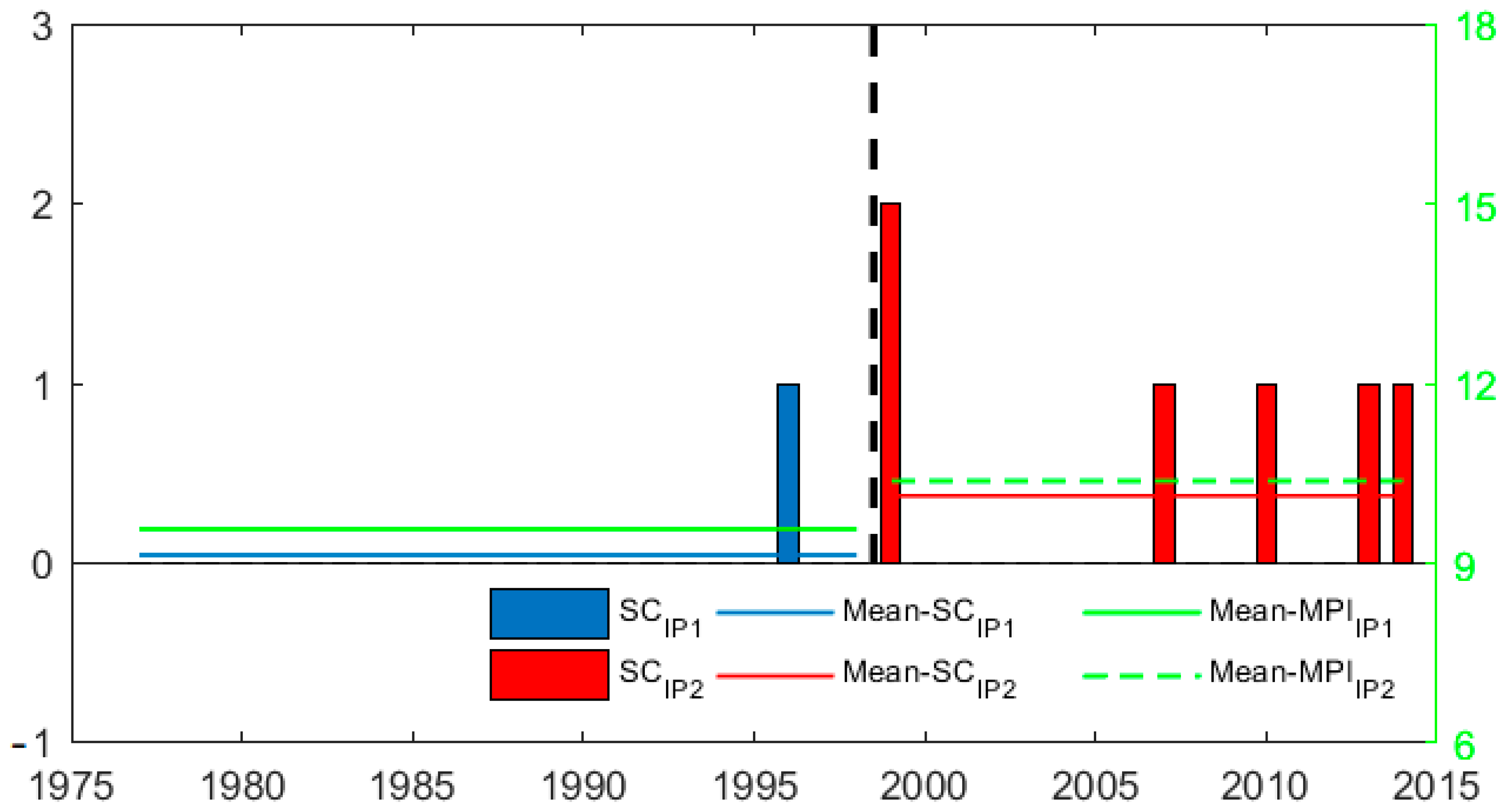
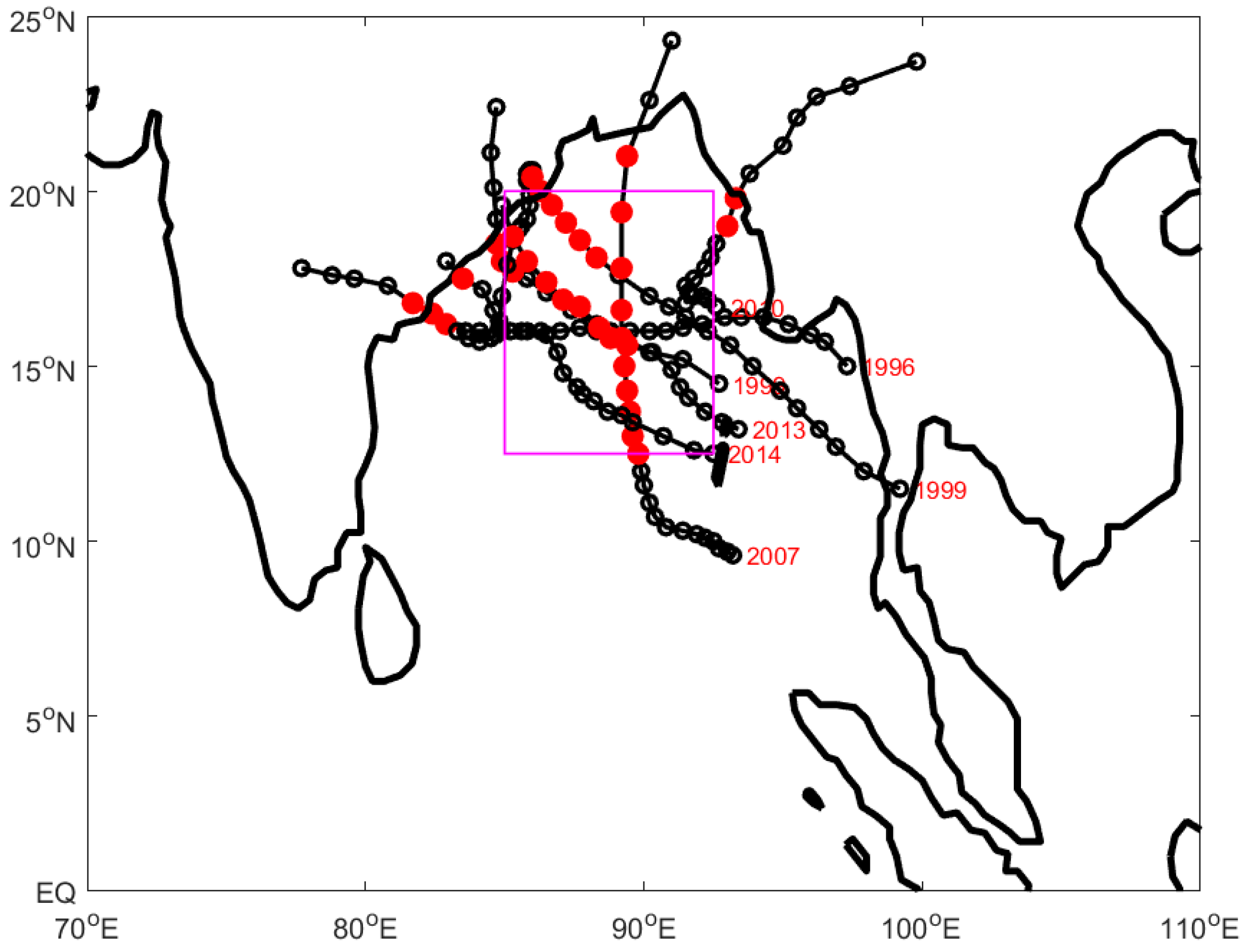
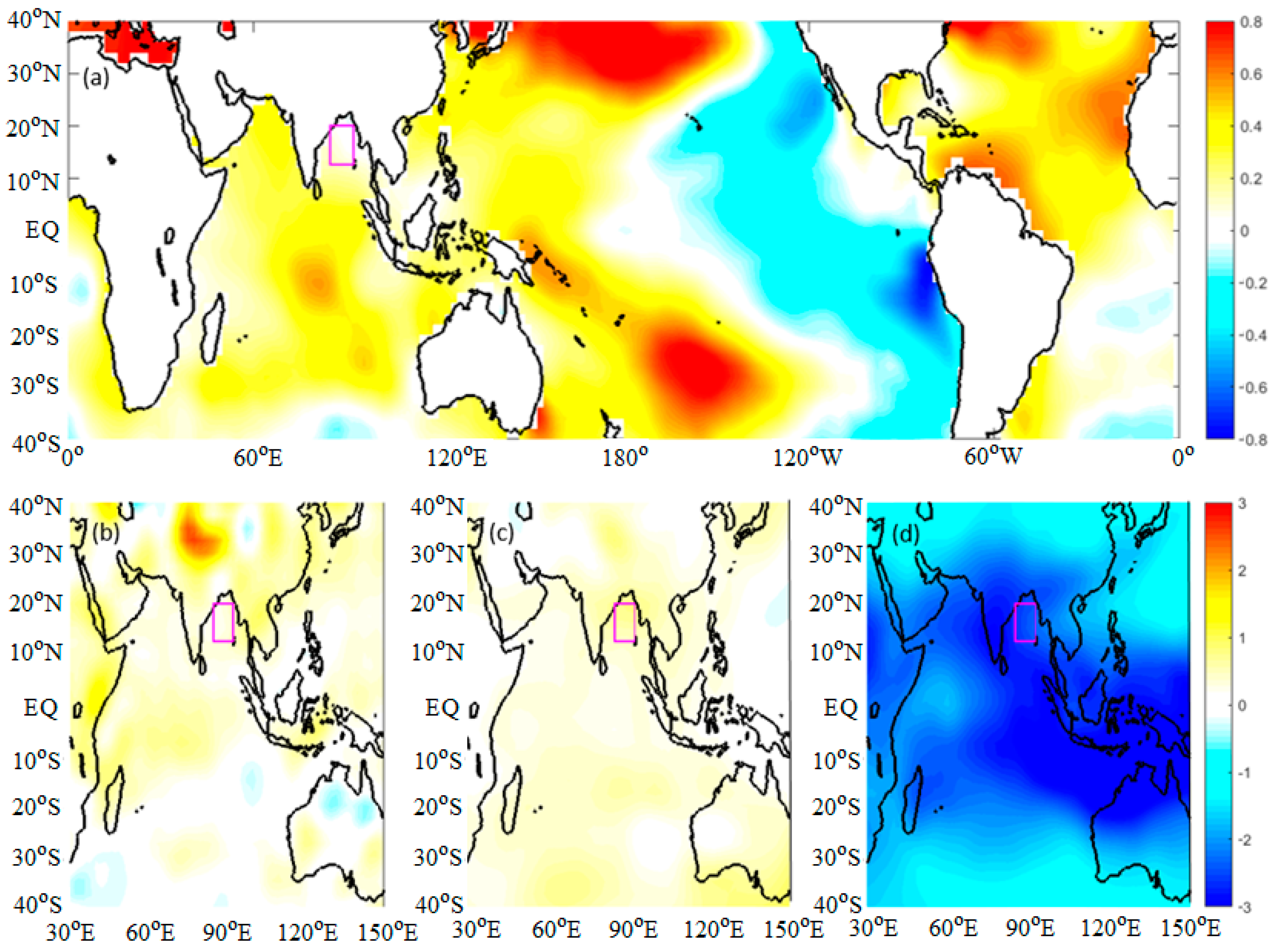
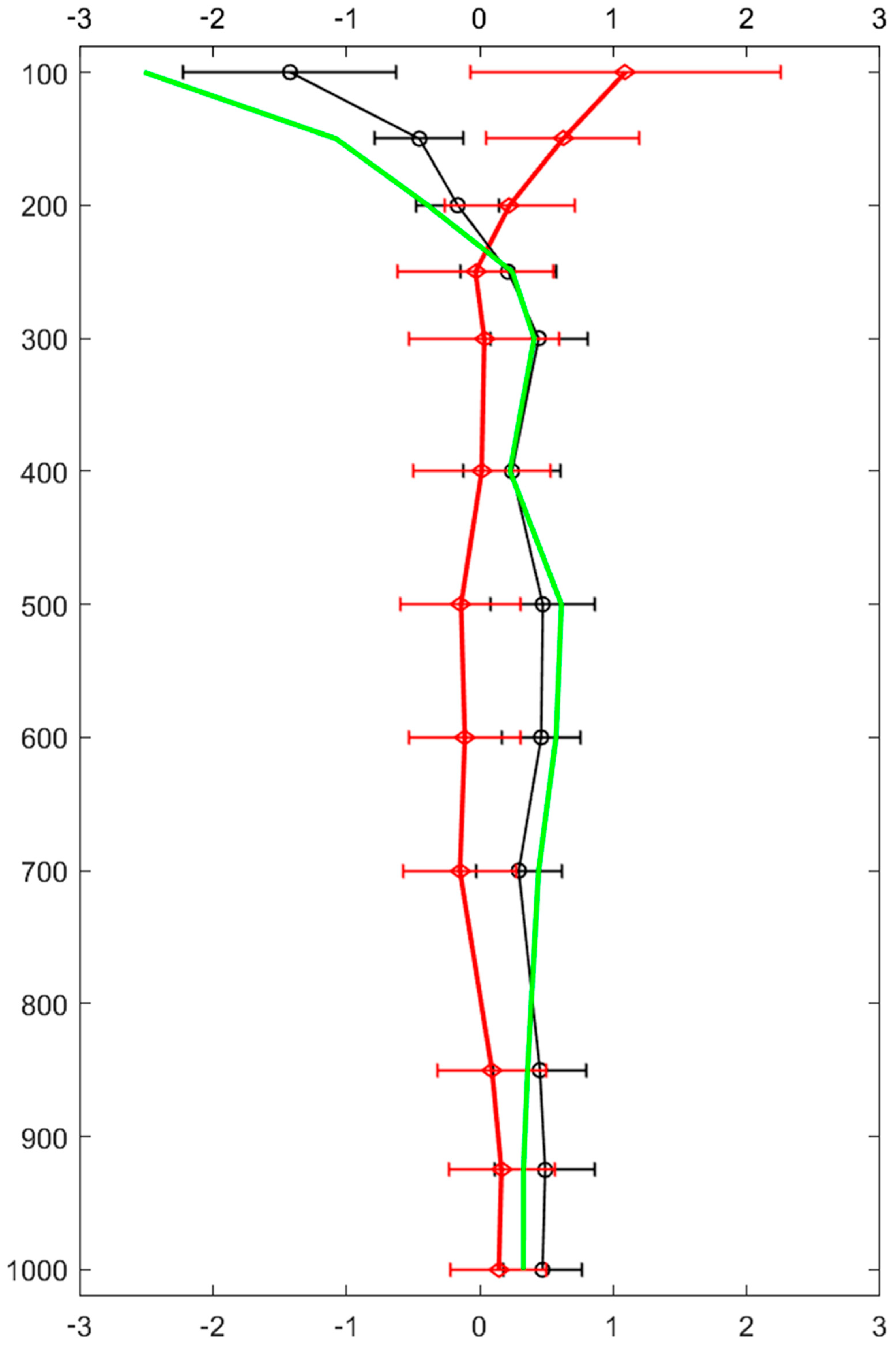
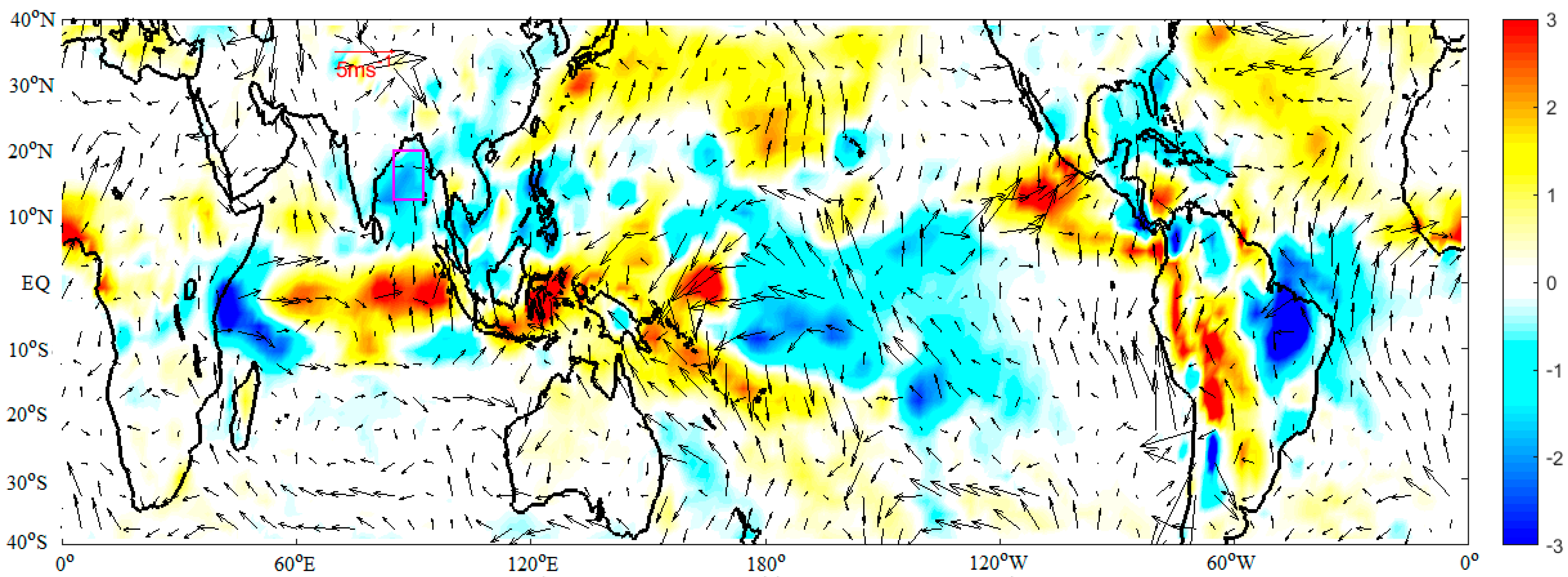
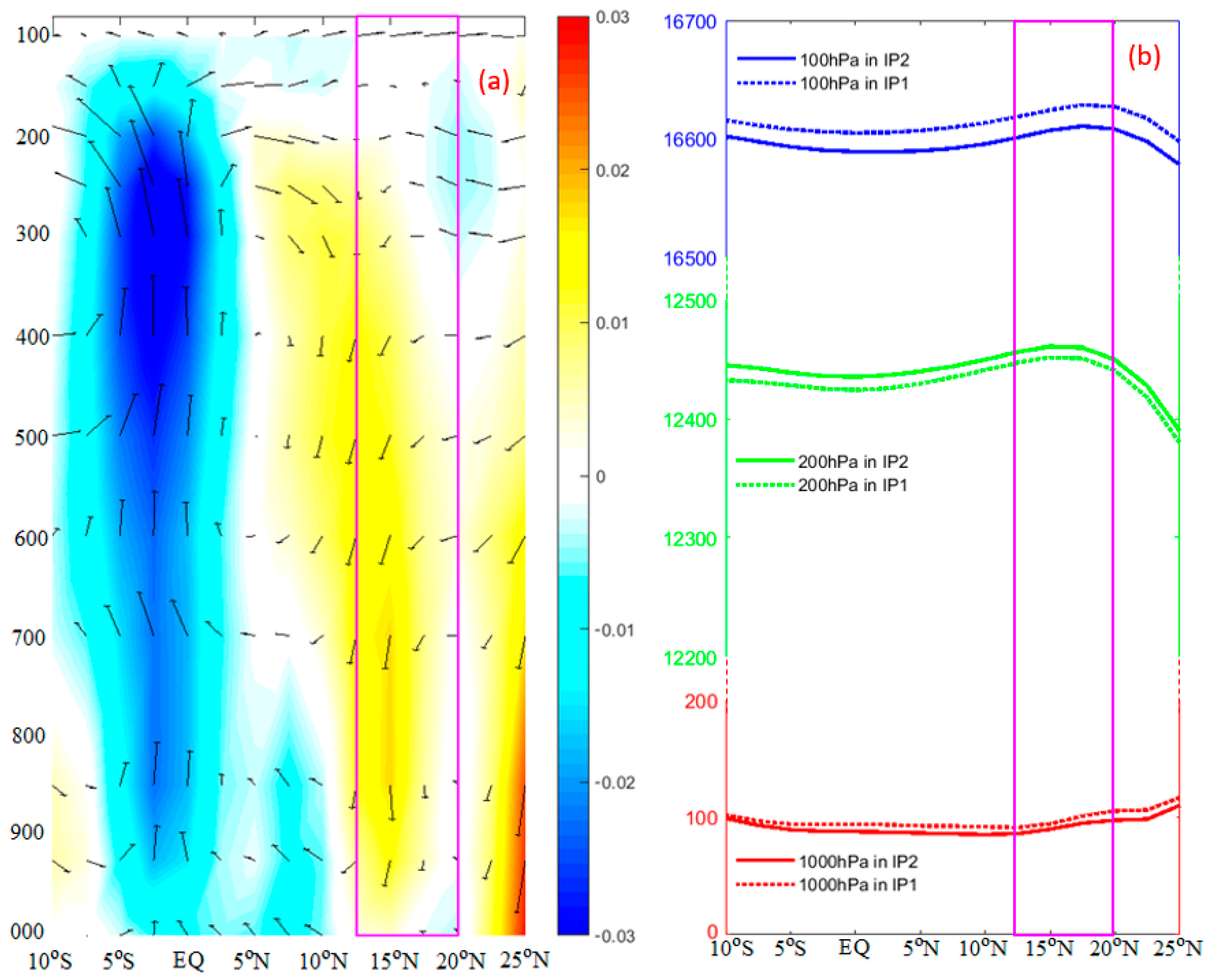
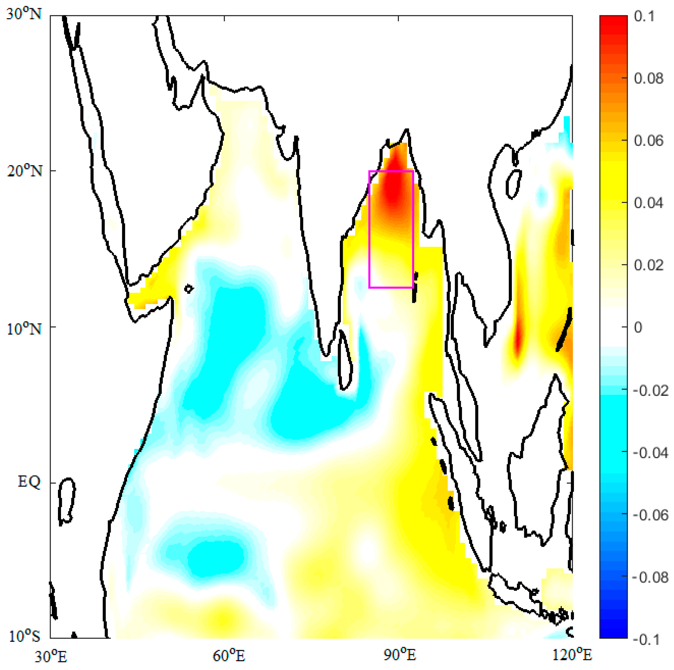
3. Analysis and Results

As was previously determined, 1977 and 1999 were key shift points for the IPO. Compared with the 1977–1998 period, the 1999–2014 period was characterized by the negative-phase IPO, and an obvious La Niña-like pattern could be observed in the Pacific Ocean at this time. Six SCs occurred over the BoB during the PS of IP2, while the annual average number of SCs that occurred during the PS of IP2 was in stark contrast with that recorded in IP1 (Figure 1), which was approximately 8 times more in IP2 than in IP1. According to the tracks of these SCs, the region of 7.5–20° N and 85–92.5° E is regarded as the reference area in this study to carry a diagnostic analysis on the differences in SC activities between the two periods (Figure 2).

Similar to the difference observed in the average annual numbers of SCs between IP1 and IP2, the reference-box-averaged V_pot² values, which could effectively mirror the MPI values [18], also significantly differed between IP2 and IP1 at the 95% confidence level. The components of V_pot², such as T_vd, T_vr and T_ed, also revealed some differences at significance levels greater than 99%, more than 99% and less than 90%, respectively (

Table 1. Differences in the studied terms between IP2 and IP1, their corresponding significance levels and the relative contributions of the changes in various terms to ΔV_pot².

	${\mathit{V}}_{\mathit{p}\mathit{o}\mathit{t}}^2$	Tvd	Tvr	Ted
IP2-IP1	>0	>0	>0	>0
Significance of difference	>95%	>99%	>99%	<90%
		Tvd and Tvr		Ted
$\mathrm{The}\mathrm{proportion}\mathrm{of}\mathrm{the}\mathrm{contribution}\mathrm{to}\Delta V_{pot}^2$		89%		11%

). Hence, V_pot² can be regarded as a diagnostic equation with which the contributions of environmental factors associated with MPI to the SC differences between IP2 and IP1 can be quantitatively analyzed.

The diagnostic results show that the greatest contribution to the observed difference in SC activities between the PS periods in IP2 and IP1 was provided by the T_vd and T_vr terms. Because T_vd and T_vr are determined only by the surface and outflow temperatures, their effects could be regarded together. Table 1 illustrates that most of the contribution came from T_vd and T_vr, which together accounted for approximately 89% of the contribution (Table 1). T_ed provided only approximately 11% of the contribution to ΔV_pot² (Table 1). We could also conclude that surface and outflow temperatures may be the most important environmental factors modulating the remarkable observed difference.

To further verify the diagnostic results described above and quantitatively contrast the changes observed in other environmental factors, such as the T, vorticity (Vor), ω, VWS, RH and SH, affecting TC genesis and development [38,42,43], we introduced the BDI to quantitatively adjust the differences in the environmental factors with different units. The diagnosis results are listed in

Table 2. BDI values of each environmental factor considered in the reference at multiple atmospheric levels during the PS.

BDI (IP2-IP1)	1000	925	850	700	600	500	400	300	200	100
Vor	−0.17	−0.11	−0.05	0.02	0.15	0.11	0.09	0.24	0.30	−0.01
ω	0.03	0.31	0.34 *	0.39 *	0.39 *	0.32	0.25	0.13	−0.04	−0.58 *
T	0.50 *	0.43 *	0.47 *	0.59 *	0.80 *	0.73 *	0.24	0.44 *	−0.48 *	−1.28 *
RH	−0.35	−0.14	−0.11	−0.33	−0.37 *	−0.62 *	−0.62 *	−0.89 *
SH	0.05	0.06	0.08	−0.20	−0.23	−0.47 *	−0.51 *	−0.66 *

Note: the * symbol indicates that the significance level is >95%.

. T was significantly different between IP2 and IP1 at almost every level, especially at the 100 hPa level (Table 2). Although the mid-level RH and SH were lower in IP2 than in IP1, they mainly affected the genesis of TCs rather than the intensity. Given that the boundary-layer SH was slightly more abundant in IP2 than in IP1, this factor naturally had little influence on the observed difference in TC intensity (Table 2).

Based on the above analysis of the diagnostic results, we thought that T, especially upper-level T, may have been the most critical factor that determined the different SC formation mechanisms between IP2 and IP1. Hence, we further analyzed the SST data and the 3-dimensional T structure. Except for an obvious La Niña-like pattern in the Eastern Pacific, warming could be observed almost basin-wide in the tropical Indian Ocean between the PS of IP2 and IP1 (Figure 3a). The bottom- and middle-level (1000- and 500 hPa-level) T warming values nearly fit the SST differences observed in the tropical Indian Ocean (Figure 3b,c), and the corresponding BDIs were 0.50 and 0.73, respectively (Table 2). The upper-level (100 hPa-level) T was evidently colder in IP2 than in IP1, particularly in the Indo-Pacific warm pool region (Figure 3d), and the corresponding BDI was −1.28. Therefore, among the studied factors, the difference in upper-level T might play the most important role in the atmospheric stability differences observed between IP2 and IP1.

In the reference area, the composites of T with climatology removed for IP1 and IP2 showed values of 0.14 °C and 0.47 °C, respectively, at the 1000 hPa level; and of 1.09 °C and −1.42 °C, respectively, at the 100 hPa level (Figure 4). The T differences between IP2 and IP1 were 0.33 °C and −2.51 °C at the 1000 hPa and 100 hPa levels, respectively. The vertical temperature difference (VTD) composite values obtained for IP2 and IP1 were approximately −0.95 °C and 1.89 °C, respectively, and the VTD difference between IP2 and IP1 was 2.84 °C. This obvious disparity in the VTD could induce a remarkable difference in the MPI between IP2 and IP1 with a significance level above 95%, and might further modulate the differential SC formation between IP2 and IP1. It is worth noting that this remarkable VTD difference should be mostly derived from the upper-level T difference between the PS periods of IP2 and IP1 (Figure 4). The vertical temperature ratio (VTR) has a similar result because the VTR is also determined by the lower and upper levels. These analysis results further confirm the above conclusion that the upper-level T difference is thought to be the most important environmental factor affecting the differential SC formation between the PS periods in IP2 and IP1.

Determining the reason for the very significantly negative difference observed in T at the 100 hPa level between the PS periods of IP2 and IP1 naturally became the key objective we investigated next. It is known that a La Niña-like pattern could strengthen the Walker circulation in the Pacific [44,45]. We found that under the La Niña-like SST difference that occurred during the PS periods between IP2 and IP1, the Walker circulation was enhanced in the tropical Pacific Ocean. In response to this enhanced Walker circulation in the Pacific, the other Walker circulation cell over the Indian Ocean also became stronger in IP2 than it was in IP1. The strengthening Walker circulation cells induced bottom-level westerly and easterly wind differences over the tropical Indian Ocean and Pacific Ocean and increased precipitation over the Java Sea and its adjacent regions in the maritime continent (Figure 5). Unlike the increase in precipitation observed over the eastern tropical Indian Ocean, especially in the region west of the island of Sumatra, the precipitation lessened in the BoB in IP2 compared to that measured in IP1 (Figure 5). Simultaneously, the bottom-level wind spanned the equator from the BoB and converged in the tropical southeast Indian Ocean, with a positive precipitation difference (Figure 5). All of these results imply that the local Hadley circulation might play an important role in modulating T changes over the BoB.

A detailed analysis of the along-latitude vertical motion profile was, therefore, carried out next. The 85°−92.5° E-averaged composite results show an anomalous ascending motion that is consistent with the enhanced convection observed in the western region of Sumatra. This ascending branch is well connected to a descending branch over the BoB through a local anomalous Hadley circulation (Figure 6a). The high-pressure difference at the 200 and 300 hPa level coincides with the descending difference; this correspondence may result from convergence in the upper troposphere. In contrast with the 200 hPa level, low pressure is observed at the 100 hPa level above the descending branch. High- and low-pressure centers arise corresponding to positive and negative potential height changes, respectively, according to the hydrostatic relationship. Figure 6b shows a negative potential height change at 100 hPa but a positive potential height change at 200 hPa. Naturally, the 100 hPa level becomes anomalously cold due to the reduced thickness between the 100 hPa and 200 hPa levels.

Through the above analyses, we could comprehend the mechanism by which the observed high-level negative temperature difference formed between IP2 and IP1, and then sought to understand the physical process that modulated the significant increase in the number of SC occurrences during the PS period in IP2 from the atmospheric dynamics and thermodynamics perspectives. In addition to the possible effects of atmospheric processes, the ocean, as the underlying surface of TC activities, also established favorable conditions for enhanced TC intensities over the BoB during the PS in IP2 compared to those in IP1. Heating in the central and eastern tropical Indian Ocean and the westerly wind difference below this heating force a downwelling Kelvin wave to propagate eastward along the equator; then, this Kelvin wave moves along the rim of the BoB as a coastal Kelvin wave (Figure 7). Furthermore, the Kelvin wave in the eastern BoB radiates westward as a downwelling Rossby wave and enters the interior of the BoB. This poleward-propagating coastally downwelling Kelvin wave and the westward-propagating downwelling Rossby wave effectively deepen the thermocline in the BoB during the PS periods in IP2 (Figure 7). This thickened thermocline results in an enlarged upper-ocean heat content [46,47] and a more stable stratification of the upper Ocean; these conditions are favorable to TC intensification. The processes described in this study jointly construct favorable atmospheric and oceanic conditions that ultimately result in the significant difference observed in SC activities over the BoB during the PS periods between IP2 and IP1.

4. Conclusions

The IPO experienced positive and negative phases during the 1977–1998 (IP1) and 1999–2014 (IP2) periods, respectively. Compared to IP1, an obvious La Niña-like pattern occupied the tropical Pacific during IP2, and this pattern even impacted the global climate in some sense through teleconnections. As a possible response to this La Niña-like pattern, approximately 8 times more annual average SC incidences occurred over the BoB during the PS periods in IP2 than in IP1.

Our analysis indicates that the La Niña-like pattern strengthens the Walker circulation and then enhances convection in the central and eastern tropical Indian Ocean, especially in the area west of Sumatra. The enhanced convection in the southeast Indian Ocean induces a local anomalous Hadley circulation, and the descending branch of this circulation is located over the BoB, causing a high-pressure center at the 300 hPa level. Simultaneously, a low-pressure center occurs above the descending branch at approximately the 100 hPa level. According to the hydrostatic relationship, the 100 hPa low-pressure center and 200 hPa high-pressure center could effectively reduce the thickness between the 100 and 200 hPa levels and cause a remarkable negative T difference at the upper level between IP2 and IP1. Furthermore, a relatively small positive T difference can be observed at the bottom level, and this difference may be associated with the positive SST difference observed in the BoB between IP2 and IP1. All of these results support the positive differences observed in T_vd and T_vr between IP2 and IP1. Certainly, these positive differences can be mainly attributed to the upper-level T difference between the two periods. Finally, these differences could affect the MPI difference and even modulate the differential annual average number of recorded SCs between the PS periods of IP2 and IP1.

In addition, the positive heating and westerly wind differences observed between IP2 and IP1 cause the downwelling Kelvin wave to propagate eastward along the equator. This Kevin wave traverses the rim of the BoB as a coastal Kelvin wave and deepens the thermocline in the BoB. Then, the Kelvin wave is reflected at the eastern coast of the BoB into the downwelling Rossby wave that enters the interior of the BoB and increases the thermocline depth in this region. This deep thermocline is also favorable for TC intensification.

The combination of atmospheric and oceanic conditions analyzed in this study ultimately modulate the significant differences in SC activities observed over the BoB between the PS periods of IP2 and IP1. This study has important significance as a reference for understanding and predicting SCs over the BoB.

References

1. Emanuel, K.A. Tropical cyclones. Annu. Rev. Earth Planet. Sci. 2003, 31, 75–104. [Google Scholar] [CrossRef]
2. Pielke, R.A., Jr.; Gratz, J.; Landsea, C.W.; Collins, D.; Saunders, M.A.; Musulin, R. Normalized hurricane damage in the United States: 1900–2005. Nat. Hazards Rev. 2008, 9, 29–42. [Google Scholar] [CrossRef]
3. Blake, E.S.; Landsea, C.W.; Gibney, E.J. The Deadliest, Costliest, and Most Intense United States Tropical Cyclones from 1851 to 2010 (and Other Frequently Requested Hurricane Facts); NOAA Technical Memorandum NWS NHC-6; National Oceanic and Atmospheric Administration, National Weather Service, National Hurricane Center: Miami, FL, USA, 2011. [Google Scholar]
4. Wahiduzzaman, M.; Oliver, E.C.J.; Wotherspoon, J.S.; Holbrook, N.J. A climatological model of North Indian Ocean tropical cyclone genesis, tracks and landfall. Clim. Dyn. 2017, 49, 2585–2603. [Google Scholar] [CrossRef]
5. Wahiduzzaman, M.; Oliver, E.C.J.; Klotzbach, P.J.P.; Wotherspoon, J.S.; Holbrook, N.J. A statistical seasonal forecast model of North Indian Ocean tropical cyclones using the quasi-biennial oscillation. Int. J. Climatol. 2019, 39, 934–952. [Google Scholar] [CrossRef]
6. Wahiduzzaman, M.; Oliver, E.C.; Wotherspoon, S.; Luo, J.J. Statistical forecasting of tropical cyclones over the North Indian Ocean and the role of El Niño-Southern Oscillation. Clim. Dyn. 2020, 54, 1571–1589. [Google Scholar] [CrossRef]
7. Wahiduzzaman, M.; Yeasmin, A.; Luo, J.J.; Quadir, D.A.; Amstel, A.V.; Cheung, K. Markov Chain Monte Carlo simulation and regression approach guided by El Niño–Southern Oscillation to model the tropical cyclone occurrence over the Bay of Bengal. Clim. Dyn. 2021, 56, 2693–2713. [Google Scholar] [CrossRef]
8. Wahiduzzaman, M.; Cheung, K.; Luo, J.-J.; Bhaskaran, P.K.; Tang, S.; Yuan, C. Impact assessment of Indian Ocean Dipole on the North Indian Ocean tropical cyclone prediction using a Statistical model. Clim. Dyn. 2022, 58, 1275–1292. [Google Scholar] [CrossRef]
9. Needham, H.; Keim, B.; Sathiaraj, D. A Review of Tropical Cyclone-Generated Storm Surges: Global Data Sources, Observations and Impacts: A Review of Tropical Storm Surges. Rev. Geophys. 2015, 53, 545–591. [Google Scholar] [CrossRef]
10. Webster, P.J. Myanmar’s deadly daffodil. Nat. Geosci. 2008, 1, 488–490. [Google Scholar] [CrossRef]
11. Kikuchi, K.; Fudeyasu, H. Genesis of tropical cyclone Nargis revealed by multiple satellite observations. Geophys. Res. Lett. 2009, 36, L06811. [Google Scholar] [CrossRef] [Green Version]
12. Lin, I.I.; Chen, C.H.; Pun, I.F.; Liu, W.T.; Wu, C.C. Warm ocean anomaly, air sea fluxes, and the rapid intensification of Tropical Cyclone Nargis (2008). Geophys. Res. Lett. 2009, 36, L03817. [Google Scholar] [CrossRef] [Green Version]
13. McPhaden, M.J.; Foltz, G.R.; Lee, T.; Murty, V.S.N.; Ravichandran, M.; Vecchi, G.A.; Vialard, J.; Wiggert, J.D.; Yu, L. Ocean–atmosphere interactions during Cyclone Nargis. EOS Trans. Am. Geophys. Union 2009, 90, 53. [Google Scholar] [CrossRef]
14. Yanase, W.; Taniguchi, H.; Satoh, M. The genesis of tropical cyclone Nargis (2008): Environmental modulation and numerical predictability. J. Meteorol. Soc. Jpn. 2010, 88, 497–519. [Google Scholar] [CrossRef] [Green Version]
15. Yanase, W.; Satoh, M.; Taniguchi, H.; Fujinami, H. Seasonal and intraseasonal modulation of tropical cyclogenesis environment over the Bay of Bengal during the extended summer monsoon. J. Clim. 2012, 25, 2914–2930. [Google Scholar] [CrossRef] [Green Version]
16. Li, Z.; Yu, W.; Li, T.; Murty, V.S.N.; Tangang, F. Bimodal character of cyclone climatology in Bay of Bengal modulated by monsoon seasonal cycle. J. Clim. 2013, 26, 1033–1046. [Google Scholar] [CrossRef]
17. Akter, N.; Tsuboki, K. Role of synoptic scale forcing in cyclogenesis over the Bay of Bengal. Clim. Dyn. 2014, 43, 2651–2662. [Google Scholar] [CrossRef]
18. Mcphaden, M.J.; Lee, T.; Mcclurg, D. El Nino and its relationship to changing background conditions in the tropical Pacific Ocean. Geophys. Res. Lett. 2011, 38, 175–188. [Google Scholar] [CrossRef]
19. Saji, N.H.; Goswami, B.N.; Vinayachandran, P.N.; Yamagata, T. A dipole mode in the tropical Indian Ocean. Nature 1999, 401, 360–363. [Google Scholar] [CrossRef]
20. Webster, P.J.; Moore, A.M.; Loschnigg, J.P.; Leben, R.R. Coupled ocean–atmosphere dynamics in the Indian Ocean during 1997–98. Nature 1999, 401, 356–360. [Google Scholar] [CrossRef]
21. Wang, B.; Chan, J.C.L. How strong ENSO events affect tropical storm activity over the western North Pacific. J. Clim. 2002, 15, 1643–1658. [Google Scholar] [CrossRef]
22. Ho, C.H.; Kim, J.H.; Jeong, J.H.; Kim, H.S.; Chen, D. Variation of tropical cyclone activity in the South Indian Ocean: El Nino-South Oscillation and Madden-Julian Oscillation effects. J. Geophys. Res. 2006, 111, D22101. [Google Scholar] [CrossRef] [Green Version]
23. Camargo, S.J.; Emanuel, K.A.; Sobel, A.H. Use of a genesis potential index to diagnose ENSO effects on tropical cyclone genesis. J. Clim. 2007, 20, 4819–4824. [Google Scholar] [CrossRef]
24. William, M.F.; Young, S.G. The interannual variability of tropical cyclones. Mon. Weather Rev. 2007, 135, 3587–3598. [Google Scholar]
25. Eric, K.W.; Chan, J.C.L. Interannual variations of tropical cyclone activity over north Indian Ocean. Int. J. Climatol. 2012, 32, 819–830. [Google Scholar]
26. Li, Z.; Yu, W. Modulation of Interannual Variability of TC activity over Southeast Indian Ocean by Negative IOD Phase. Dyn. Atmos. Oceans 2015, 72, 62–69. [Google Scholar] [CrossRef]
27. Girishkumar, M.S.; Ravichandran, M. The influences of ENSO on tropical cyclone activity in the Bay of Bengal during October-December. J. Geophys. Res. 2012, 117, C02033. [Google Scholar] [CrossRef]
28. Singh, O.P.; Gupta, M.; Santha, K.; Saikia, D.; Khanuja, S. Indian Ocean dipole mode and tropical cyclone frequency. Curr. Sci. 2008, 94, 29–31. [Google Scholar]
29. Yuan, J.P.; Cao, J. North Indian Ocean tropical cyclone activities influenced by the Indian Ocean Dipole mode. Sci. China Earth Sci. 2013, 56, 855–865. [Google Scholar] [CrossRef]
30. Li, Z.; Li, T.; Yu, W.; Li, K.; Liu, Y. What Controls the Interannual Variation of Tropical Cyclone Genesis Frequency over Bay of Bengal in the Post-Monsoon Peak Season? J. Atmos. Sci. 2016, 17, 148–154. [Google Scholar] [CrossRef] [Green Version]
31. Wang, B. Interdecadal changes in El Niño onset in the last four decades. J. Clim. 1995, 8, 267–285. [Google Scholar] [CrossRef] [Green Version]
32. Mantua, N.J.; Hare, S.R.; Zhang, Y.; Wallace, M.J.; Francis, C.R. A Pacific interdecadal climate oscillation with impacts on salmon production. Bull. Am. Meteorol. Soc. 1997, 78, 1069–1079. [Google Scholar] [CrossRef]
33. Hu, F.; Li, T.; Liu, J. Cause of interdecadal change of tropical cyclone controlling parameter in the western North Pacific. Clim. Dyn. 2018, 51, 719–732. [Google Scholar] [CrossRef]
34. Yao, S.; Luo, J.; Huang, G.; Wang, P. Distinct global warming rates tied to multiple ocean surface temperature changes. Nat. Clim. Chang. 2017, 7, 486–491. [Google Scholar] [CrossRef]
35. Knapp, K.R.; Kruk, M.C.; Levinson, D.H.; Diamond, J.H.; Neumann, J.C. The international best track archive for climate stewardship (IBTrACS) unifying tropical cyclone data. Bull. Am. Meteorol. Soc. 2010, 91, 363–376. [Google Scholar] [CrossRef]
36. Kalnay, E.; Kanamitsu, M.; Kistler, R.; Collins, W.; Deaven, D.; Gandin, L.; Iredell, M.; Saha, S.; White, G.; Woollen, J.; et al. The NCEP/NCAR 40-year reanalysis project. Bull. Am. Meteorol. Soc. 1996, 77, 437–471. [Google Scholar] [CrossRef] [Green Version]
37. Bister, M.; Emanuel, K.A. Low frequency variability of tropical cyclone potential intensity 1. Interannual to interdecadel variability. J. Geophys. Res. 2002, 107, 4801. [Google Scholar] [CrossRef]
38. Emanuel, K.A.; Nolan, D.S. Tropical cyclone activity and the global climate system. In Proceedings of the 26th Conference on hurricanes and tropical meteorology, Miami, FL, USA, 3–7 May 2004. [Google Scholar]
39. Fu, B.; Peng, S.M.; Li, T.; Stevens, D. Developing versus nondeveloping disturbances for tropical cyclone formation, Part II: Western North Pacific. Mon. Weather Rev. 2012, 140, 1067–1080. [Google Scholar] [CrossRef] [Green Version]
40. Peng, S.M.; Fu, B.; Li, T.; Stevens, D.E. Developing versus nondeveloping disturbances for tropical cyclone formation. Part I: North Atlantic. Mon. Weather Rev. 2012, 140, 1047–1066. [Google Scholar] [CrossRef] [Green Version]
41. Li, Z.; Li, T.; Yu, W. Environmental conditions regulating the formation of super tropical cyclone during pre-monsoon transition period over Bay of Bengal. Clim. Dyn. 2019, 52, 3857–3867. [Google Scholar] [CrossRef]
42. Gray, W.M. Global view of the origin of tropical disturbances and storms. Mon. Weather Rev. 1968, 96, 669–700. [Google Scholar] [CrossRef]
43. Murakami, H.; Wang, B. Future change of North Atlantic tropical cyclone tracks: Projection by a 20-km-mesh global atmospheric model. J. Clim. 2010, 23, 2699–2721. [Google Scholar] [CrossRef]
44. Collins, M.; An, S.; Cai, W.; Ganachaud, A.; Guilyardi, E.; Jin, F.F.; Jochum, M.; Lengaigne, M.; Power, S.; Timmermann, A.; et al. The impact of global warming on the tropical Pacific Ocean and El Niño. Nat. Geosci. 2010, 3, 391–397. [Google Scholar] [CrossRef]
45. DiNezio, P.N.; Clement, A.C.; Vecchi, G.A. Reconciling differing views of tropical Pacific climate change. EOS Trans. Am. Geophys. Union 2010, 91, 141–142. [Google Scholar] [CrossRef] [Green Version]
46. Yu, L. Variability of the depth the 20 °C isotherm along 6°N in the Bay of Bengal: Its response to remote and local forcing and its relation to satellite SSH variability. Deep Sea Res. Part II 2003, 50, 2285–2304. [Google Scholar] [CrossRef]
47. Girishkumar, M.S.; Prakash, V.; Ravichandran, M. Influence of Pacific Decadal Oscillation on the relationship between ENSO and tropical cyclone activity in the Bay of Bengal during October–December. Clim. Dyn. 2015, 44, 3469–3479. [Google Scholar] [CrossRef]
Figure 1. Statistical analysis of SCs over the BoB during the PS in IP1 (1977–1998 year) and IP2 (1999–2014 year). The blue bar is the SC frequency in IP1, which is the annual average number of SCs. Similar to the symbols used for IP1, the red symbols denote IP2. The solid and dashed green lines denote the average maximum potential intensity (MPI) values in the PS of IP1 and IP2, respectively.
Atmosphere 13 00685 g001
Figure 2. Center tracks of SCs during PS of IP1 and IP2 over the BoB. The red dot means TC speed reaches categories 4 and 5.
Atmosphere 13 00685 g002
Figure 3. Composite differences in SST and T during the PS between IP2 and IP1: (a) the SST difference (unit: °C); (bd) the T differences at the 1000 hPa, 500 hPa and 100 hPa levels, respectively (unit: °C). The red box is the reference area in the BoB.
Atmosphere 13 00685 g003
Figure 4. Composite profiles of T with climatology removed, showing the standard errors and differences between IP2 and IP1 (unit: °C). The red line is the box-averaged temperature measured in IP1, the red stem is the standard error, the black line and stem are the corresponding values measured in IP2 and the green line is the temperature difference between IP2 and IP1.
Atmosphere 13 00685 g004
Figure 5. Composite differences in the precipitation rate (shading, unit: kg m−2 s−1) and 1000 hPa-level wind (vector, unit: m s−1) during the PS between IP2 and IP1. The red box is the reference area in the BoB.
Atmosphere 13 00685 g005
Figure 6. Meridional-vertical section of the 85°−92.5° E-averaged composite difference in vertical motion (shading) and the overturning circulation (vector) in PS between IP2 and IP1: (a) the vectors represent the zonal velocity (unit: m s1) and vertical velocity (unit: Pa s1); (b) the potential heights of 1000, 200 and 100 hPa levels in IP1 and IP2 (unit: m).
Atmosphere 13 00685 g006
Figure 7. Composite SSH difference (shading, unit: m) during the PS between IP2 and IP1. The red box is the reference area in the BoB.
Atmosphere 13 00685 g007