
Tropical Cyclone Intensity Prediction Using Deep Convolutional Neural Network


1
School of the Environment, Nanjing University, Nanjing 210046, China
2
School of the Environment, Nanjing Normal University, Nanjing 210023, China
3
Net Zero Era (Jiangsu) Environmental Technology Co., Ltd., Suzhou 215000, China
*
Author to whom correspondence should be addressed.
Atmosphere 2022, 13(5), 783; https://0-doi-org.brum.beds.ac.uk/10.3390/atmos13050783
Submission received: 12 April 2022
/
Revised: 6 May 2022
/
Accepted: 10 May 2022
/
Published: 12 May 2022
(This article belongs to the Special Issue Investigating Tropical Cyclone Intensity Changes with Advanced Data Analysis Techniques)
Abstract
:In this study, deep convolutional neural network (CNN) models of stimulated tropical cyclone intensity (TCI), minimum central pressure (MCP), and maximum 2 min mean wind speed at near center (MWS) were constructed based on ocean and atmospheric reanalysis, as well Best Track of tropical hurricane data over 2014–2018. In order to explore the interpretability of the model structure, sensitivity experiments were designed with various combinations of predictors. The model test results show that simplified VGG-16 (VGG-16 s) outperforms the other two general models (LeNet-5 and AlexNet). The results of the sensitivity experiments display good consistency with the hypothesis and perceptions, which verifies the validity and reliability of the model. Furthermore, the results also suggest that the importance of predictors varies in different targets. The top three factors that are highly related to TCI are sea surface temperature (SST), temperature at 500 hPa (TEM_500), and the differences in wind speed between 850 hPa and 500 hPa (vertical wind shear speed, VWSS). VWSS, relative humidity (RH), and SST are more significant than MCP. For MWS and SST, TEM_500, and temperature at 850 hPa (TEM_850) outweigh the other variables. This conclusion also implies that deep learning could be an alternative way to conduct intensive and quantitative research.
1. Introduction
Tropical cyclone (TC), one of the most severe weather systems which develop over the tropical ocean, have been drawing large attention due to their devastating impact on human beings [1]. It has been found that the intensity of TC mainly depends on three factors [2]: the initial intensity of TC, the thermodynamic state of the atmosphere, and the heat exchange between the ocean and TCs. However, it is still difficult to predict TC intensity (TCI) accurately due to the limited understanding of TC dynamics and sparse observation over the ocean [3,4]. More importantly, TC has shown 13~15% intensifying trend over the past 37 years, since the late 1970s, [5] and the current situation is not optimistic. Therefore, it is essential to develop advanced models to better understand and predict TCI, as their associated destructive winds, extreme precipitation [6,7], floods [8], landslides [9], and other drastic disasters are threatening human life and property.
Based on atmospheric processes and variables, numerous models have been constructed to predict the track of a TC and TCI. Predicting models can generally be divided into two types: numerical models and statistical models. Numerical models heavily rely on complex physical processes to forecast TCI and its track. Shao and Smith [10] improved the prediction of hurricanes Florence and Michael by assimilating atmospheric retrievals from hyperspectral instruments into the Weather Research and Forecasting (WRF) system. Such processes need to deal with a large amount of data and cost intensive computation resources. Furthermore, the poor understanding of complex physical processes, the inaccurate vortex initialization, and large calculation process hinder numerical models’ ability to simulate precisely and efficiently [11].
Considering the constraints of numerical models, statistical models are more flexible and consume fewer computational resources, opening up new opportunities for growth under the prosperity of big data. To some extent, traditional statistical models such as standard multiple regression [12], Generalized Additive Model (GAM) [13], and Statistical Hurricane Intensity Prediction Scheme (SHIPS) [14] could be used to predict TCs. Nevertheless, ordinary non-linear regression still has a limited ability to describe non-linear relations.
With the development of machine learning methods, especially the appearance of neural networks with activation functions, various advanced models have been employed to forecast TCs. Sen et al. [15] applied an Artificial Neural Network (ANN) to improve the performance of non-linear autoregressive models that forecast cyclone disturbances. Furthermore, deep learning techniques such as using a Convolutional Neural Network (CNN), which was designed to process images exclusively, have been widely applied to learn features from satellite imagery data [16,17]. Pradhan et al. [18] designed CNN based on LeNet-5 [19] to extract features from satellite imagery and estimated TCI. To achieve a more accurate prediction, deeper networks were employed and more information was integrated and fed into the network. Higa et al. [20] applied complicated Visual Geometry Group Network-16 (VGG-16) to capture more features from the satellite imagery of TC. Giffard-Roisin et al. [21] constructed fused deep learning models consisting of two CNN modules to learn from wind fields and geopotential height fields. However, most of this research focused on satellite imagery and ignored the importance of atmospheric and ocean data. Zhang et al. [22] considered nine predictors when building CNN, e.g., brightness, temperature, relative vorticity, and geopotential height (GEOPH), but the sea surface temperature (SST) was not included. In this case, more factors that have direct or substantial impacts on TC should be taken into consideration, such as SST [23,24] and vertical wind shear (VWS) [25], which can more effectively identify and affect the dynamic and thermodynamic processes of the interaction between ocean and TCs. Additionally, the interpretability study of machine learning is a new field that verifies the reliability of models. However, models are hardly applied to conduct interpretability experiments and some researchers ignore the importance of ‘visualizing’ the black box. Correspondingly, having an in-depth understanding of model results improves our perspective on the importance of factors and the mechanisms of TC formation.
In this paper, data and the model construction are described in Section 2. Briefly, 2014–2018 atmospheric and ocean reanalysis data are used to construct the predicting model, which is based on the simplified version of VGG-16 (VGG-16s) [26]. Then, we evaluate its performance by comparing it with two other underlying CNN models in Section 3.1. Moreover, we extend the application for an in-depth understanding of the interpretability of our model results by analyzing the importance of variables in Section 3.2.
2. Data and Methods
2.1. Data
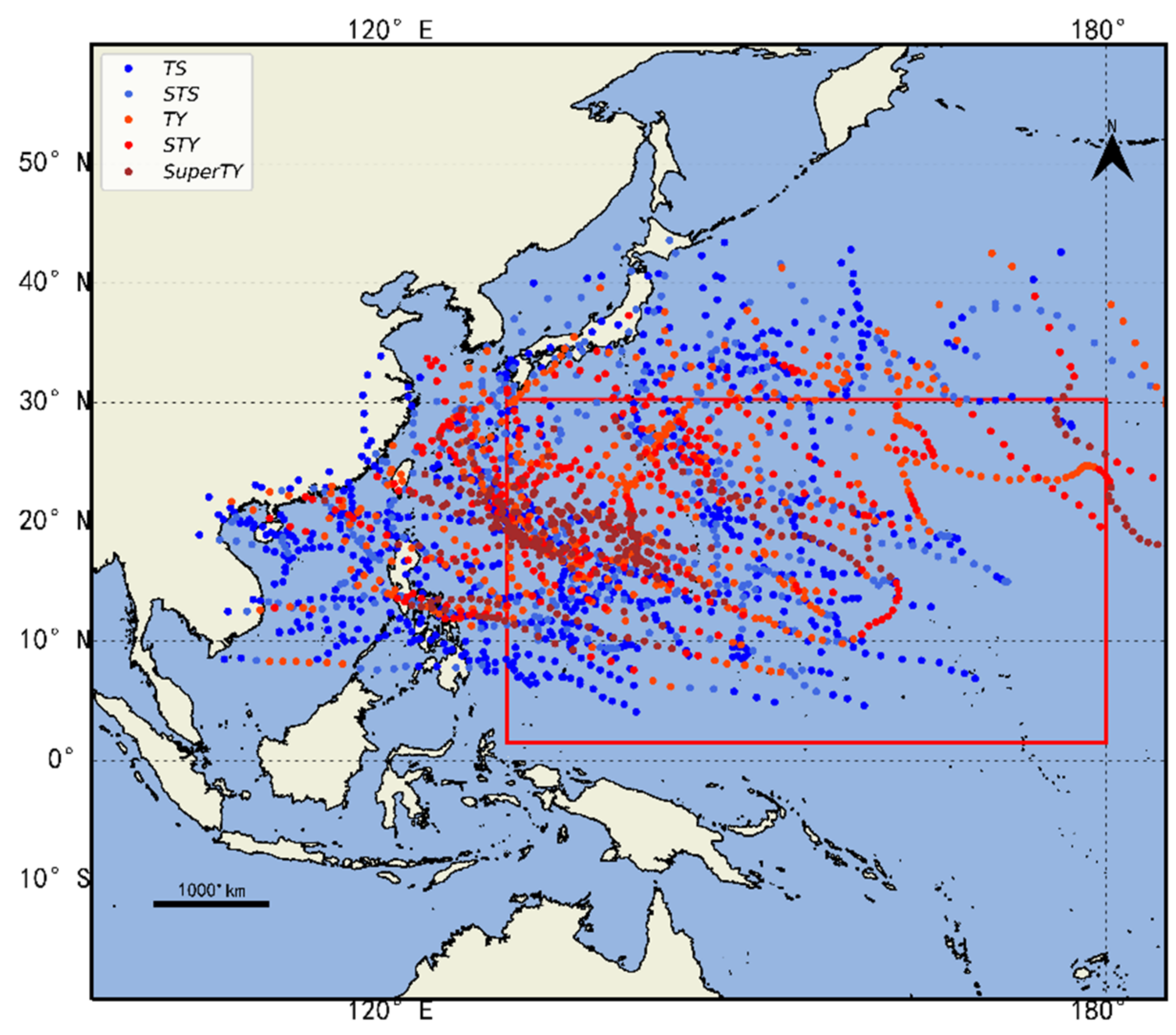
The fifth generation of atmospheric reanalysis from ECMWF (ERA5) ranging from 2014 to 2018 was used to provide necessary meteorological and ocean predictors in our research. The temporal and horizontal resolutions of ERA5 are 3 h and 0.25° × 0.25°, respectively. We mainly focused on the TCs that entered the region with latitude ranges between 1.5° N and 30.25° N and longitude ranges between 129.75° E and 180° E, which mainly consists of the Northwest Pacific Ocean, as shown in the red box in Figure 1. Target data of 6 h intervals within the study region, including TCI, minimum central pressure (MCP), and maximum 2 min mean wind speed at near center (MWS), were obtained from Best Track (BT) data from the China Meteorological Administration Tropical Cyclone Data Center, Beijing [27,28] and data are available at http://tcdata.typhoon.org.cn/en/zjljsjj_sm.html (accessed on 15 February 2022). In order to keep the coherency of data structure, we pre-processed the input feature and target data into the same temporal resolution (6 h). Ten predictors were utilized in the model: SST, temperature at 850 and 500 hPa (TEM_850 and TEM_500), the average of divergence (DIV) at 850 hPa and 1000 hPa, GEOPH at 850 hPa, relative humidity (RH) at 1000 hPa, meridional and zonal components of wind speed (V and U, respectively) at 850 hPa, and VWS between 500 and 850 hPa. It is noted that the VWS is characterized by the differences of wind speed and wind direction between 850 hPa and 500 hPa (VWSS and VWSD, respectively). In addition, U and V contain the information of TC central wind speed and TCI. In other words, U and V are not independent variables to the target TCI and MWS. Therefore, these two factors were not considered as the model predictors nor as sensitivity experiments targeting TCI and MWS. For different targets, the predictors used in the experiment are shown in Table 1. Five-year data from 2014 to 2018 were used to train, validate, and test the model. In the shuffled dataset, a total of 2970 samples were obtained. Of these, 60% of the data made up training dataset, 20% made up validation dataset, and 20% made up testing dataset.
2.2. Model
Generally, CNN comprises of the convolutional layer, the pooling layer, the fully connected layer, and the non-linear activation function. Focusing on the ‘deep in’ neural network, Simonyan and Zisserman [26] created VGG-16 with 13 convolutional layers to classify high-resolution images. Deeper layers can avoid missing features but also increase the number of parameters. Thus, a smaller kernel of 3 × 3 size is utilized to improve efficiency. Owing to the limitation of sample size, we reduced the number of convolutional layers to 10, resulting in the simplified VGG-16 (VGG-16s).
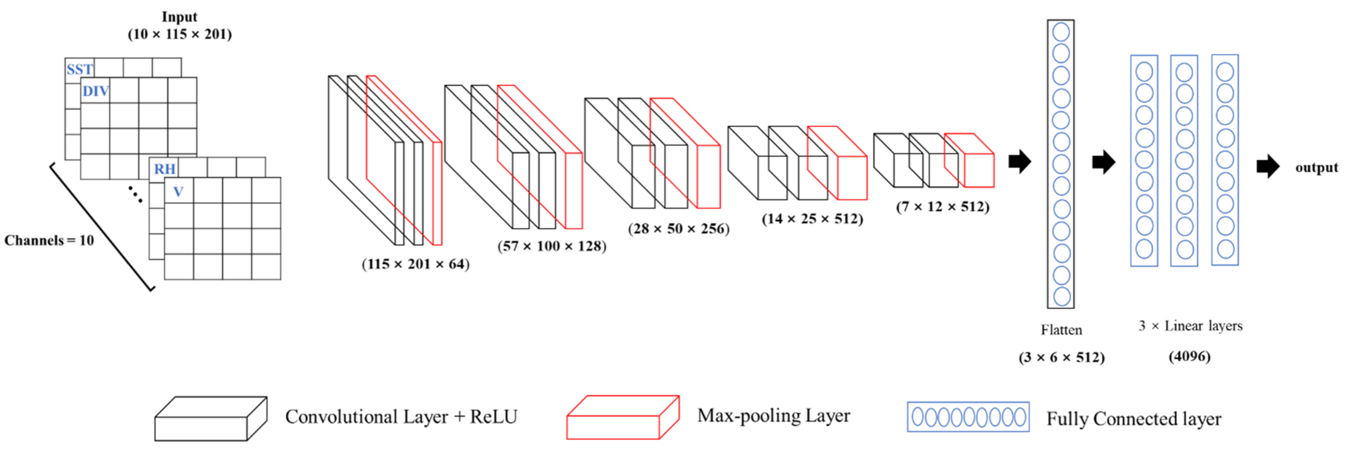
The architecture of VGG-16s is shown in Figure 2. Before feeding data into the network, data are organized into four dimensions, which are samples, feature types, the height of the feature map, and the width of the feature map. The spatial grids of each feature can be seen as a channel of the picture, so the shape of input sample is 10 (8 for TCI) × 115 × 201. For the first convolutional block, 64 filters of 3 × 3 size are used to extract features. After that, the max pooling layer performs down-sampling and reduces the feature map size to 57 × 100. For the second, third, fourth, and fifth convolutional blocks, feature maps are processed similarly. There are 128, 256, 512, and 512 filters of 3 × 3 kernel size to capture features and the size of feature maps are, respectively, reduced to 28 × 50, 14 × 25, 7 × 12, and 3 × 6 after max pooling. We used the ReLU function as the activation function and the padding option was applied to avoid missing information. Then, the 3D matrix of 3 × 6 × 512 size was flattened into a vector of 9216 size, and three fully connected neural networks with 4096 nodes are utilized to output the target.
2.3. Experiment Set-Up
In this paper, the VGG-16s was developed and two classical CNN models were chosen to evaluate the performance of VGG-16s, which are LeNet-5 and AlexNet [29]. LeNet-5 has the initial structure of complex CNN models, which combines the pooling layer and the convolution layer. Additionally, it is designed to accomplish simple-image recognition tasks such as identifying handwritten numbers. The modules of AlexNet and LeNet-5 are quite similar. However, AlexNet has 1000 times more parameters to learn than LeNet-5. Consequently, dropout layers are employed to prevent overfitting. To further avoid overfitting, early stopping was applied to find the best epoch and the dropout number was set to 0.5. Learning rate was chosen by learning rate decay strategy. Other parameters are shown in Table 2.
Then, we used the VGG-16s model to carry out experiments and tried to explore the difference of predictor importance among the three targets. In detail, sensitivity experiments were conducted relying on training a few models with different predictors. For MCP and MWS, experiments were designed by training models based on removing one predictor each time. The differences of test results from different runs revealed the importance of the removed predictors. Furthermore, the change range of metrics could measure the importance magnitude. For TCI, experiments were designed by using one predictor to train the model each time. For example, if the model trained with SST outperforms the model trained with RH, SST possibly outweighs RH for TCI.
To evaluate the performance of models on test datasets, coefficients of determination (R2), root mean square error (RMSE), mean absolute error (MAE), and symmetric mean absolute percentage error (SMAPE) were used for the regression task. On the basis of their definition, the lower the MAE, RMSE, and SMAPE are, the better the model will be. Accuracy (ACC), precision (Pre), recall (Rec), and F1-score (F1) are metrics for the classification task.
ACC is the proportion of correctly classified samples in total samples:
where represents the number of samples that were correctly classified; represents the number of total test samples.
Pre indicates the proportion of true positive results in all positive results. In a certain category, the calculation formula is as follows:
where represents the number of samples that were correctly classified as true category; represents the number of samples that were incorrectly classified as true category.
Rec is the number of true positive samples divided by original positive samples. In a certain category, the calculation formula is as follows:
where represents the number of samples that were incorrectly classified as the false categories.
To balance Pre and Rec, F1 is utilized to combine these two indexes. If F1 is high, both the precision and recall of the classifier indicate good results. In a certain category, the calculation formula is as follows:
In summary, ACC is used to measure the model performance on overall samples. Pre and Rec are complementary metrics to assess judgement errors based on the positive prediction results and judgement omissions based on true positive values. F1 is designed to integrate Pre and Rec. In addition, Pre, Rec, and F1 are based on the number of TCI levels, which is seven in this study. Thus, the macro-average method, which calculates average values of all categories, was used to integrate.
3. Results
3.1. Model Comparison
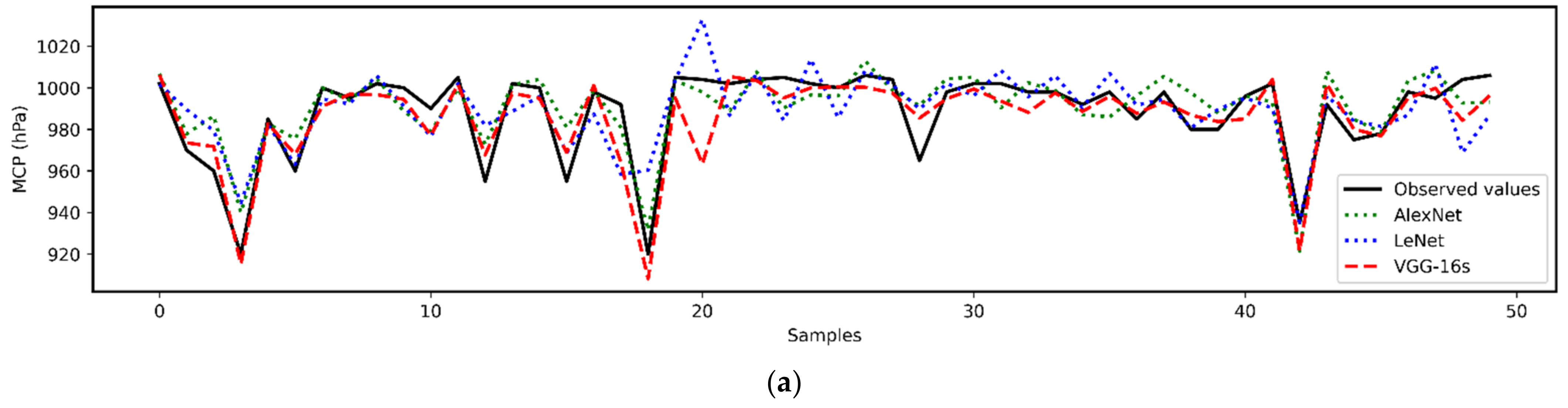
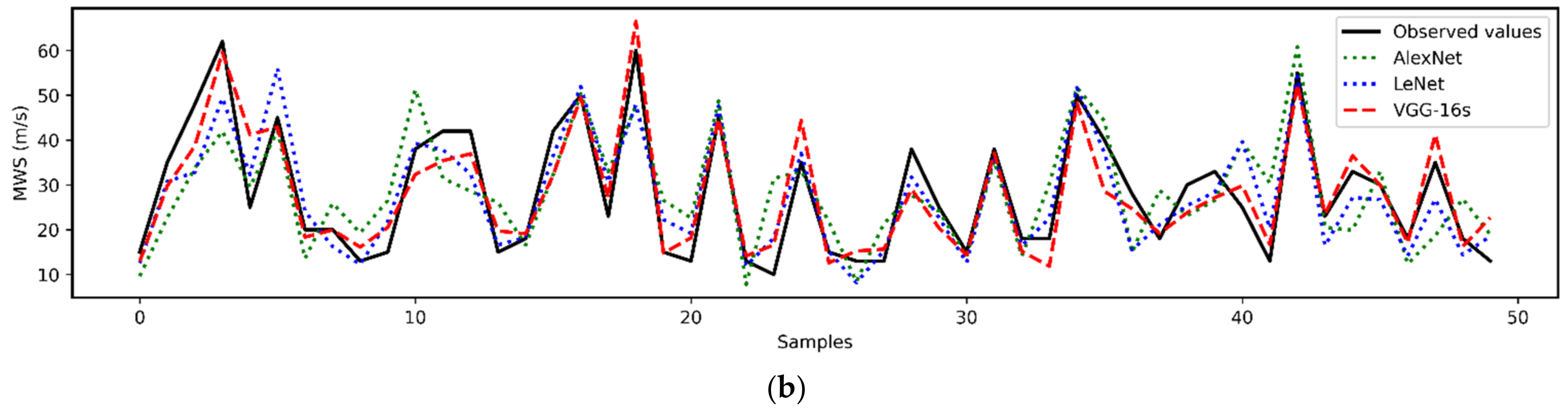
The estimation metrics of different models when predicting three selected targets are shown in Table 3. Generally, VGG-16s achieved a better prediction performance with three targets than the other two models. Especially in comparison to LeNet-5, the R2 of VGG-16s increased by 33%, and RMSE, MAE, and SMAPE of VGG-16s, respectively, reduced by 30%, 36%, and 36% for the MCP forecast. In terms of predicting MWS, the improvements shown on four indices (R2, RMSE, MAE and SMAPE) are 31%, 35%, 41%, and 39% compared to LeNet-5. Figure 3 shows the comparison between the observed values and prediction results of MCP and MWS from three models. It was found that the prediction results of VGG-16s (the red dashed lines) are closer to the observed values (the black solid lines) than the prediction results of LeNet-5 and AlexNet, which are consistent with the metrics results. Such improvements indicate that deeper layers could help the model capture more details and can deal with multi-channels consisting of various factors.
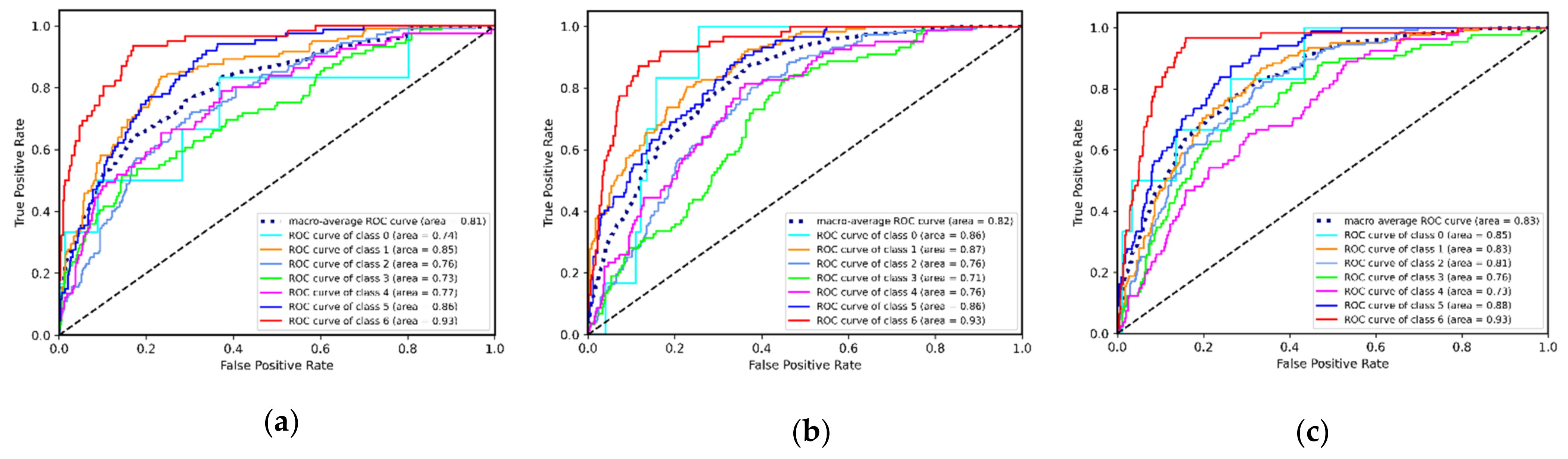
However, VGG-16s showed a slightly superior performance when classifying TCI. Compared with LeNet-5, four indicators increased by 15%, 5.8%, 18%, and 10%, respectively. This smaller improvement is possibly due to the insufficient predictors, the imbalance of samples, and inadequate model structure. Therefore, the model needs to be further optimized and more predictors need to be selected to achieve further improvements. In addition, the macro-average Receiver Operating Characteristic (ROC) [30] curves and ROC curves of different categories of three models are shown in Figure 4. It manifests that the area under the macro-average ROC curve elevates gradually and VGG-16s has the best classification performance on major classes. In summary, VGG-16s performs better than LeNet-5 and AlexNet with regard to the project of three targets. Thus, VGG-16s is applied to sensitivity experiments.
3.2. Sensitivity Experiments
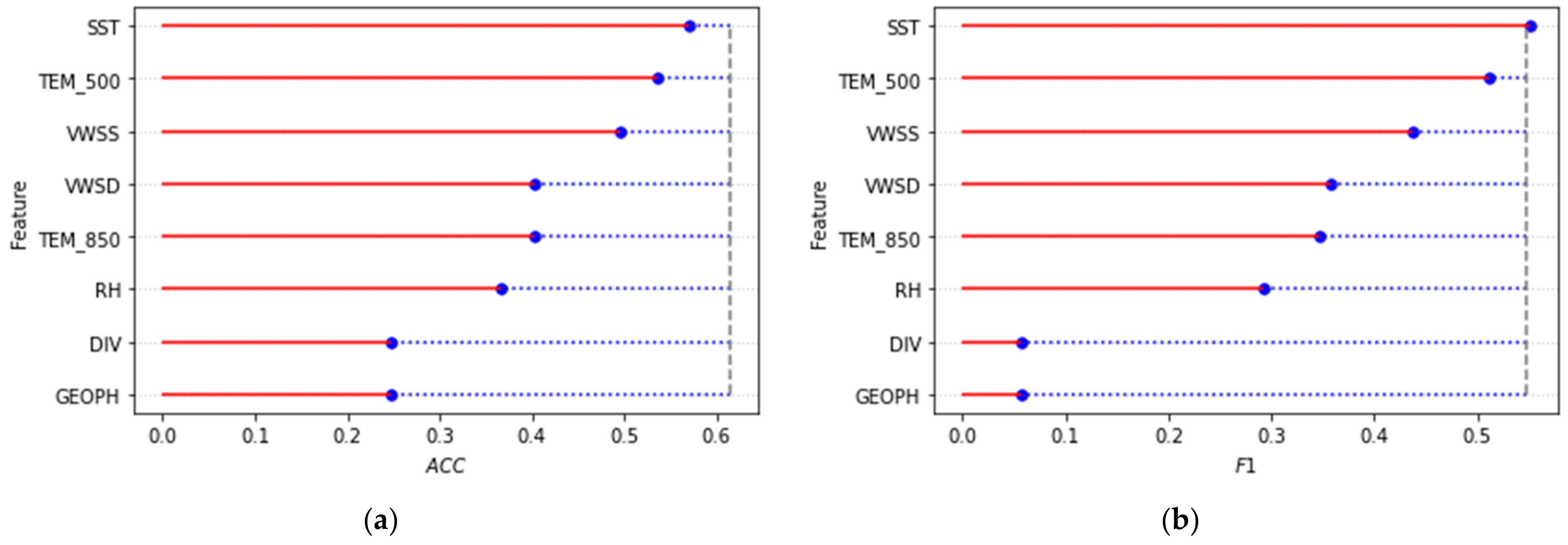
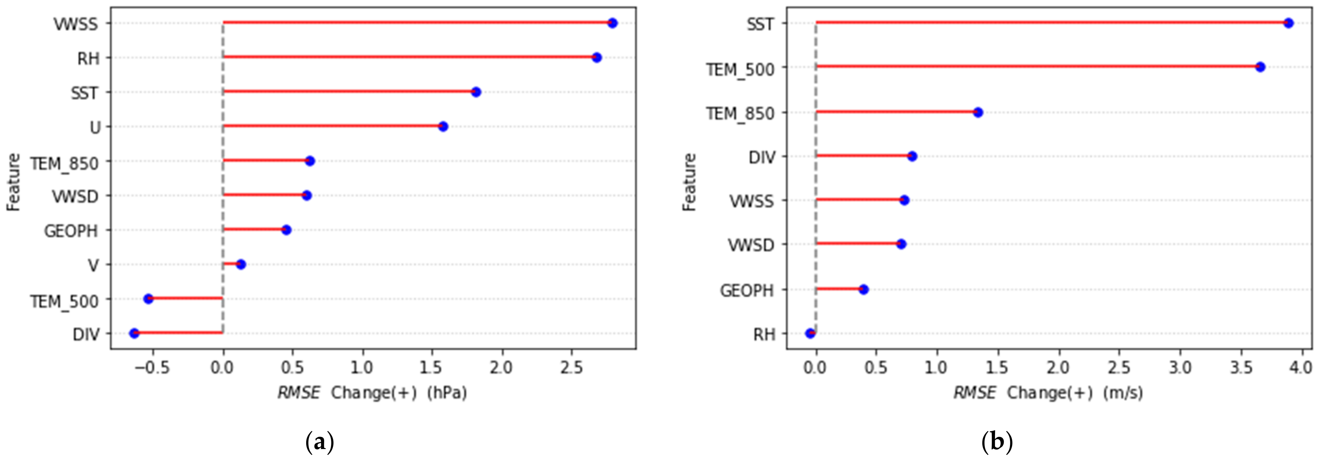
The sensitivity results are shown in Figure 5 and Figure 6. The results show that SST, VWSS, and TEM_500 are the top three important factors in TCI predictions. VWSS, RH, and SST make the most contributions to MCP among the selected factors. SST, TEM_500, and TEM_850 are the top three factors exhibiting closer relations to MWS. Common features can be found in the sensitivity results among three targets. Firstly, SST is a critical variable for three targets, which is due to the fact that ocean potential heat is a crucial energy resource to the formation and enhancement of TC. Generally, a high SST can be seen as a signal that a large amount of water in the ocean evaporates into the atmosphere, which is favorable to a low-pressure center and intensifying TC [23,31,32]. Secondly, TEM_500 is important for both MWS and TCI. This can be attributed to the moisture budget and heat exchange. When wet air mass rises, it releases latent heat that warms the surroundings to keep a warm core. After that, dry air continues rising and become colder. Therefore, the lower the upper air temperature, the more latent heat is released at around 500 hPa, which is possibly similar to the characteristic of outflow temperature [33,34]. Thirdly, VWSS has a high sensitivity to MCP and TCI, which is potentially related to the ventilation effect [35]. A deeper VWS may induce the upper and lower layers of TC to be in different phases, disrupting the energy transport and weakening the warm core. Consequently, a high VWSS is not conducive to TC intensification and is usually seen as a key factor impeding the development of TC. Furthermore, VWS is of great significance to MCP, which suggests that VWS may more directly influence a low-pressure center. Additionally, it is noted that GEOPH is not quite vital to the predicted three targets, especially to TCI and MWS. A possible explanation is that GEOPH is more likely to impact TC track than intensity [36]. Moreover, some differences are expected among three targets, particularly between MCP and MWS. This result indicates that RH is more important to MCP than the other two targets. Statistical data show that TC rapid intensification cases have higher values of 850~700 hPa relative humidity [37]. Areas with a high RH may imply violent evaporation, strong air–sea interaction cycle, and deep lowering of the pressure field [32]. In contrast, vertical temperature distribution is significant for MWS. However, a few previous works focused on the relations between temperature at certain layers and MWS. Therefore, this problem must be further investigated by numerical models.
4. Discussion
A precise TC forecast model could help to identify risks and reduce the loss caused by TCs. In this paper, we compared three basic CNN models based on ocean, atmospheric, and TC data, and VGG-16s was found to perform well. More advanced models such as ResNet [38] and efficient methods such as Synthetic Minority Over-sampling Technique (SMOTE) [39] and Under-sampling (US) [40] that deal with small samples problem should be considered and used to improve model performance, especially for classification tasks. Additionally, the integrated models which combine the merits and function of numerical weather forecast models and machine learning models are possibly meaningful to the development of TC forecasting. Moreover, selecting the best predictor group is instrumental to model efficiency. For example, studies indicate that the tropical cyclone heat potential (TCHP) is more closely related to the central pressure than SST [41]. Therefore, TCHP is possibly a more crucial factor to be chosen as a predictor. Currently, an excessive and insufficient input could bring high computation and poor performance. Thus, choosing the appropriate method when selecting factors is vital.
Studying interpretability is also critical to convince decision makers and researchers to apply models with confidence. In this study, we explored the interpretability of VGG-16s. The results display how the deep learning model makes predictions on targets, which is an alternative way to make structures more visible and explainable. Furthermore, interpretability techniques of deep learning are worthy of being further studied, not merely focusing on factor importance. For instance, saliency maps [42] are promising to explore the spatial patterns of features.
Scenario studies could be carried out based on advanced models. In this research, an interpretability analysis also provides a reference for finding the most direct impact of TC and identifying the priority of function route of TC. Although some preliminary conclusions were found, various issues are still difficult to understand and elucidate comprehensively. In essence, deep learning is still a black box which adds difficulties to mechanism study. Consequently, it is a vital and profound direction for deep research to not only expand the study field of interpretability, but also to consider how to integrate numerical models.
5. Conclusions
In summary, VGG-16s with 10 convolution layers was constructed to stimulate the TCI, MCP, and MWS of TCs. Then, we compared VGG-16s with LeNet-5 and AlexNet, and the results indicate that VGG-16s outperforms the other two models on the three targets, which implies that VGG-16s is probably more appropriate to stimulate TCI, MCP, and MWS. The VGG-16s model structure was further utilized to analyze interpretability by studying sensitivity. The result suggests that the structure of VGG-16s has good interpretability and the importance of predictors varies in different targets, though three targets are all used to depict TC intensity. The top three factors which are highly related to TCI are SST, TEM_500, and VWSS. VWSS, RH, and SST are more critical to MCP. For MWS, SST, TEM_500, and TEM_850 outweigh the other variables. Additionally, the difference in rank manifests that factors have a distinct function route influencing TC intensity. More importantly, deep learning provides an alternative approach to exploring TC formation and intensification, which will bring benefits to promote a more advanced forecast system.
Author Contributions
Conceptualization, X.-Y.X. and M.S.; methodology, X.-Y.X.; software, X.-Y.X.; validation, P.-L.C.; formal analysis, X.-Y.X. and M.S.; investigation, X.-Y.X. and M.S.; resources, Q.-G.W.; data curation, X.-Y.X. and M.S.; writing—original draft preparation, X.-Y.X.; writing—review and editing, M.S.; visualization, X.-Y.X. and M.S.; supervision, M.S. and Q.-G.W.; project administration, M.S. and Q.-G.W.; funding acquisition, M.S. All authors have read and agreed to the published version of the manuscript.
Funding
This research was funded by the Natural Science Foundation of Jiangsu Province (No. BK20210574).
Institutional Review Board Statement
Not applicable.
Informed Consent Statement
Not applicable.
Data Availability Statement
ERA5 data are available at https://www.ecmwf.int/en/forecasts/datasets/reanalysis-datasets/era5 (accessed on 10 February 2022); BT data are available at http://tcdata.typhoon.org.cn/en/zjljsjj_sm.html (accessed on 15 February 2022).
Acknowledgments
The model was constructed on the basis of the VGGNet which is proposed by the University of Oxford Visual Geometry Group. The data used as predictors were provided by ECMWF and the target data were provided by China Meteorological Administration Tropical Cyclone Data Center. We appreciate the support of these institutes.
Conflicts of Interest
The authors declare no conflict of interest.
References
- Peduzzi, P.; Chatenoux, B.; Dao, H.; De Bono, A.; Herold, C.; Kossin, J.; Mouton, F.; Nordbeck, O. Global trends in tropical cyclone risk. Nat. Clim. Chang. 2012, 2, 289–294. [Google Scholar] [CrossRef]
- Emanuel, K.A. Thermodynamic control of hurricane intensity. Nature 1999, 401, 665–669. [Google Scholar] [CrossRef]
- Xu, Y.; Zhang, L.; Gao, S. The Advances and Discussions on China Operational Typhoon Forecasting. Meteorol. Mon. 2010, 36, 43–49. [Google Scholar]
- Wang, Y.; Wu, C.C. Current understanding of tropical cyclone structure and intensity changes—A review. Meteorol. Atmos. Phys. 2004, 87, 257–278. [Google Scholar] [CrossRef]
- Mei, W.; Xie, S.P. Intensification of landfalling typhoons over the northwest Pacific since the late 1970s. Nat. Geosci. 2016, 9, 753–757. [Google Scholar] [CrossRef]
- Chen, Y.; Zhai, P.M. Persistent extreme precipitation events in China during 1951–2010. Clim. Res. 2013, 57, 143–155. [Google Scholar] [CrossRef] [Green Version]
- Van Oldenborgh, G.J.; van der Wiel, K.; Sebastian, A.; Singh, R.; Arrighi, J.; Otto, F.; Haustein, K.; Li, S.H.; Vecchi, G.; Cullen, H. Attribution of extreme rainfall from Hurricane Harvey, August 2017. Environ. Res. Lett. 2017, 12, 124009. [Google Scholar] [CrossRef]
- Jonkman, S.N.; Maaskant, B.; Boyd, E.; Levitan, M.L. Loss of life caused by the flooding of New Orleans after Hurricane Katrina: Analysis of the relationship between flood characteristics and mortality. Risk Anal. Off. Publ. Soc. Risk Anal. 2009, 29, 676–698. [Google Scholar] [CrossRef]
- Lee, C.T.; Huang, C.C.; Lee, J.F.; Pan, K.L.; Lin, M.L.; Dong, J.J. Statistical approach to storm event-induced landslides susceptibility. Nat. Hazards Earth Syst. Sci. 2008, 8, 941–960. [Google Scholar] [CrossRef] [Green Version]
- Shao, M.; Smith, W.L. Impact of Atmospheric Retrievals on Hurricane Florence/Michael Forecasts in a Regional NWP Model. J. Geophys. Res. Atmos. 2019, 124, 8544–8562. [Google Scholar] [CrossRef] [Green Version]
- Ma, L. Research Progress on China typhoon numerical prediction models and associated major techniques. Prog. Geophys. 2014, 29, 1013–1022. [Google Scholar] [CrossRef]
- Demaria, M.; Kaplan, J. A statistical hurricane intensity prediction scheme (SHIPS) for the Atlantic Basin. Weather Forecast. 1994, 9, 209–220. [Google Scholar] [CrossRef]
- Wahiduzzaman, M.; Luo, J.J. Modeling of tropical cyclone activity over the North Indian Ocean using generalised additive model and machine learning techniques: Role of Boreal summer intraseasonal oscillation. Nat. Hazards. 2022, 111, 1801–1811. [Google Scholar] [CrossRef]
- DeMaria, M.; Mainelli, M.; Shay, L.K.; Knaff, J.A.; Kaplan, J. Further improvements to the Statistical Hurricane Intensity Prediction Scheme (SHIPS). Weather Forecast. 2005, 20, 531–543. [Google Scholar] [CrossRef] [Green Version]
- Sen, S.; Nayak, N.C.; Mohanty, W.K. Long-term forecasting of tropical cyclones over Bay of Bengal using linear and non-linear statistical models. Geojournal 2021, 86, 1–23. [Google Scholar] [CrossRef]
- Chen, B.; Chen, B.-F.; Lin, H.-T. Rotation-blended CNNs on a new open dataset for tropical cyclone image-to-intensity regression. In Proceedings of the 24th ACM SIGKDD Conference on Knowledge Discovery and Data Mining (KDD), London, UK, 19–23 August 2018; pp. 90–99. [Google Scholar] [CrossRef]
- Tan, J.; Yang, Q.; Hu, J.; Huang, Q.; Chen, S. Tropical Cyclone Intensity Estimation Using Himawari-8 Satellite Cloud Products and Deep Learning. Remote Sens. 2022, 14, 812. [Google Scholar] [CrossRef]
- Pradhan, R.; Aygun, R.S.; Maskey, M.; Ramachandran, R.; Cecil, D.J. Tropical Cyclone Intensity Estimation Using a Deep Convolutional Neural Network. IEEE Trans. Image Processing A Publ. IEEE Signal Processing Soc. 2018, 27, 692–702. [Google Scholar] [CrossRef]
- Lecun, Y.; Bottou, L.; Bengio, Y.; Haffner, P. Gradient-Based Learning Applied to Document Recognition. Proc. IEEE 1998, 86, 2278–2324. [Google Scholar] [CrossRef] [Green Version]
- Higa, M.; Tanahara, S.; Adachi, Y.; Ishiki, N.; Nakama, S.; Yamada, H.; Ito, K.; Kitamoto, A.; Miyata, R. Domain knowledge integration into deep learning for typhoon intensity classification. Sci. Rep. 2021, 11, 12972. [Google Scholar] [CrossRef]
- Giffard-Roisin, S.; Yang, M.; Charpiat, G.; Kumler Bonfanti, C.; Kegl, B.; Monteleoni, C. Tropical Cyclone Track Forecasting Using Fused Deep Learning From Aligned Reanalysis Data. Front. Big Data 2020, 3, 1–13. [Google Scholar] [CrossRef] [Green Version]
- Zhang, R.; Liu, Q.; Hang, R.; Liu, G. Predicting Tropical Cyclogenesis Using a Deep Learning Method From Gridded Satellite and ERA5 Reanalysis Data in the Western North Pacific Basin. IEEE Trans. Geosci. Remote Sens. 2022, 60, 1–10. [Google Scholar] [CrossRef]
- Wendland, W.M. Tropical storm frequencies related to sea-surface temperatures. J. Appl. Meteorol. 1977, 16, 477–481. [Google Scholar] [CrossRef] [Green Version]
- Mei, W.; Xie, S.P.; Primeau, F.; McWilliams, J.C.; Pasquero, C. Northwestern Pacific typhoon intensity controlled by changes in ocean temperatures. Sci. Adv. 2015, 1, e1500014. [Google Scholar] [CrossRef] [Green Version]
- Liang, X.J.; Li, Q.Q. Revisiting the response of western North Pacific tropical cyclone intensity change to vertical wind shear in different directions. Atmos. Ocean. Sci. Lett. 2021, 14, 100041. [Google Scholar] [CrossRef]
- Simonyan, K.; Zisserman, A. Very Deep Convolutional Networks for Large-Scale Image Recognition. arXiv 2014, 1409, 1556. [Google Scholar]
- Lu, X.Q.; Yu, H.; Ying, M.; Zhao, B.K.; Zhang, S.; Lin, L.M.; Bai, L.N.; Wan, R.J. Western North Pacific Tropical Cyclone Database Created by the China Meteorological Administration. Adv. Atmos. Sci. 2021, 38, 690–699. [Google Scholar] [CrossRef]
- Ying, M.; Zhang, W.; Yu, H.; Lu, X.Q.; Feng, J.X.; Fan, Y.X.; Zhu, Y.T.; Chen, D.Q. An Overview of the China Meteorological Administration Tropical Cyclone Database. J. Atmos. Ocean. Technol. 2014, 31, 287–301. [Google Scholar] [CrossRef] [Green Version]
- Krizhevsky, A.; Sutskever, I.; Hinton, G.E. ImageNet classification with deep convolutional neural networks. Commun. ACM 2017, 60, 84–90. [Google Scholar] [CrossRef]
- Hanley, J.A.; McNeil, B.J. The meaning and use of the area under a receiver operating characteristic (ROC) curve. Radiology 1982, 143, 29–36. [Google Scholar] [CrossRef] [Green Version]
- Emanuel, K.A. The dependence of hurricane intensity on climate. Nature 1987, 326, 483–485. [Google Scholar] [CrossRef]
- Holland, G.J. The maximum potential intensity of tropical cyclones. J. Atmos. Sci. 1997, 54, 2519–2541. [Google Scholar] [CrossRef]
- Ramsay, H.A. The Effects of Imposed Stratospheric Cooling on the Maximum Intensity of Tropical Cyclones in Axisymmetric Radiative-Convective Equilibrium. J. Clim. 2013, 26, 9977–9985. [Google Scholar] [CrossRef]
- Wang, S.; Camargo, S.J.; Sobel, A.H.; Polvani, L.M. Impact of the Tropopause Temperature on the Intensity of Tropical Cyclones: An Idealized Study Using a Mesoscale Model. J. Atmos. Sci. 2014, 71, 4333–4348. [Google Scholar] [CrossRef]
- Gray, W.M. Global view of the origin of tropical disturbances and storms. Mon. Weather Rev. 1968, 96, 669–700. [Google Scholar] [CrossRef]
- Ren, S.; Liu, Y.; Wu, G. Interactions between typhoon and subtropical anticyclone over western pacific revealed by numerical experiments. Acta Meteorol. Sin. 2007, 65, 329–340. [Google Scholar]
- Kaplan, J.; DeMaria, M. Large-scale characteristics of rapidly intensifying tropical cyclones in the North Atlantic basin. Weather Forecast. 2003, 18, 1093–1108. [Google Scholar] [CrossRef] [Green Version]
- He, K.; Zhang, X.; Ren, S.; Sun, J. Deep residual learning for image recognition. In Proceedings of the 2016 IEEE Conference on Computer Vision and Pattern Recognition (CVPR), Las Vegas, NV, USA, 27–30 June 2016; pp. 770–778. [Google Scholar] [CrossRef] [Green Version]
- Chawla, N.; Bowyer, K.; Hall, L.; Kegelmeyer, W. SMOTE: Synthetic Minority Over-sampling Technique. J. Artif. Intell. Res. (JAIR) 2002, 16, 321–357. [Google Scholar] [CrossRef]
- Gong, B.; Ordieres-Meré, J. Prediction of daily maximum ozone threshold exceedances by preprocessing and ensemble artificial intelligence techniques: Case study of Hong Kong. Environ. Model. Softw. 2016, 84, 290–303. [Google Scholar] [CrossRef]
- Wada, A.; Usui, N. Importance of tropical cyclone heat potential for tropical cyclone intensity and intensification in the western North Pacific. J. Oceanogr. 2007, 63, 427–447. [Google Scholar] [CrossRef]
- Simonyan, K.; Vedaldi, A.; Zisserman, A. Deep Inside Convolutional Networks: Visualising Image Classification Models and Saliency Maps. arXiv 2014, arXiv:1312.6034. [Google Scholar]
Figure 1.
Bounding box (red box) of ERA5 for model construction and targeted TC tracks. TS: Tropical Storm; STS: Severe Tropical Storm; TY: Typhoon; STY: Severe Typhoon; SuperTY: Super Typhoon.
Figure 1.
Bounding box (red box) of ERA5 for model construction and targeted TC tracks. TS: Tropical Storm; STS: Severe Tropical Storm; TY: Typhoon; STY: Severe Typhoon; SuperTY: Super Typhoon.

Figure 2.
The architecture of VGG-16s.

Figure 3.
Comparison between observations and predictions from three models. (a) MCP. (b) MWS.


Figure 4.
ROC curves of three models on the test results of TCI. (a) LeNet-5. (b) AlexNet. (c) VGG-16s. True Positive Rate (TPR): the percentage of actual positives that are accurately identified; False Positive Rate (FPR): the percentage of actual negatives that are incorrectly identified as positives. Higher TPR and lower FPR indicate better performance. The area under the ROC curve is also a measure of test results, where a greater area means better performance.

Figure 5.
Performance comparison results of models stimulating TCI trained with certain predictors. (a,b) show the performance results in ACC and F1, respectively. Red solid lines show the values of estimation metrics. Grey dashed lines show the performance of control models inputting all predictors. Blue dotted lines show the difference of performance between the control model and the experimental model.

Figure 6.
RMSE changes as a result of removing the corresponding predictor. (a) Result of MCP. (b) Result of MWS. Grey dashed lines: the RMSE of control model which was constructed by all predictors.
Figure 6.
RMSE changes as a result of removing the corresponding predictor. (a) Result of MCP. (b) Result of MWS. Grey dashed lines: the RMSE of control model which was constructed by all predictors.


Table 1.
The targets and their predictors.
| Target | Predictors | Number | Task Type |
|---|---|---|---|
| MCP | TEM_850,TEM_500, GEOPH, RH, SST, U, V, VWSS, VWSD | 10 | Regression |
| MWS | TEM_850,TEM_500,GEOPH, RH, SST, VWSS, VWSD | 8 | Regression |
| TCI | TEM_850,TEM_500, GEOPH, RH, SST, VWSS, VWSD | 8 | Classification |
Table 2.
Experimental design.
| Network | Target | Learning Rate | Weight Decay | Loss Function | Optimizer |
|---|---|---|---|---|---|
| LeNet-5 | MCP/MWS | 1 × 10⁻⁷ | 5 × 10⁻⁵ | MSE | Adam |
| TCI | 1 × 10⁻⁶ | 5 × 10⁻⁵ | Cross Entropy | Adam | |
| AlexNet | MCP/MWS | 2 × 10⁻⁶ | 5 × 10⁻⁵ | MSE | Adam |
| TCI | 1 × 10⁻⁵ | 5 × 10⁻⁵ | Cross Entropy | Adam | |
| VGG-16s | MCP/MWS | 8 × 10⁻⁶ | 5 × 10⁻⁵ | MSE | Adam |
| TCI | 4 × 10⁻⁶ | 5 × 10⁻⁵ | Cross Entropy | Adam |
Table 3.
The performance of three models in stimulating MCP, MWS, and TCI.
| Target | Evaluating Indicator | LeNet-5 | AlexNet | VGG-16s |
|---|---|---|---|---|
| MCP | R2 | 0.60 | 0.77 | 0.80 |
| RMSE (hPa) | 14.93 | 11.20 | 10.44 | |
| SMAPE | 1.18 | 0.87 | 0.75 | |
| MAE (hPa) | 11.54 | 8.53 | 7.34 | |
| MWS | R2 | 0.65 | 0.83 | 0.85 |
| RMSE (m/s) | 8.65 | 6.03 | 5.62 | |
| SMAPE | 26.07 | 17.56 | 15.49 | |
| MAE (m/s) | 6.82 | 4.56 | 4.16 | |
| TCI | ACC | 0.53 | 0.59 | 0.61 |
| Pre | 0.52 | 0.57 | 0.55 | |
| Rec | 0.49 | 0.57 | 0.58 | |
| F1 | 0.50 | 0.56 | 0.55 |
Publisher’s Note: MDPI stays neutral with regard to jurisdictional claims in published maps and institutional affiliations. |
© 2022 by the authors. Licensee MDPI, Basel, Switzerland. This article is an open access article distributed under the terms and conditions of the Creative Commons Attribution (CC BY) license (https://creativecommons.org/licenses/by/4.0/).
Share and Cite
MDPI and ACS Style
Xu, X.-Y.; Shao, M.; Chen, P.-L.; Wang, Q.-G. Tropical Cyclone Intensity Prediction Using Deep Convolutional Neural Network. Atmosphere 2022, 13, 783. https://0-doi-org.brum.beds.ac.uk/10.3390/atmos13050783
AMA Style
Xu X-Y, Shao M, Chen P-L, Wang Q-G. Tropical Cyclone Intensity Prediction Using Deep Convolutional Neural Network. Atmosphere. 2022; 13(5):783. https://0-doi-org.brum.beds.ac.uk/10.3390/atmos13050783
Chicago/Turabian StyleXu, Xiao-Yan, Min Shao, Pu-Long Chen, and Qin-Geng Wang. 2022. "Tropical Cyclone Intensity Prediction Using Deep Convolutional Neural Network" Atmosphere 13, no. 5: 783. https://0-doi-org.brum.beds.ac.uk/10.3390/atmos13050783
Note that from the first issue of 2016, this journal uses article numbers instead of page numbers. See further details here.