
Conifers May Ameliorate Urban Heat Waves Better Than Broadleaf Trees: Evidence from Vancouver, Canada


Department of Plant Biology and Gund Institute for Environment, University of Vermont, Burlington, VT 05405, USA
*
Author to whom correspondence should be addressed.
Atmosphere 2022, 13(5), 830; https://0-doi-org.brum.beds.ac.uk/10.3390/atmos13050830
Submission received: 1 April 2022
/
Revised: 9 May 2022
/
Accepted: 11 May 2022
/
Published: 19 May 2022
(This article belongs to the Special Issue State-of-Art in Urban Climate Projections)
Abstract
:Anthropogenic greenhouse gas emissions are increasing the frequency of deadly heat waves. Heat waves are particularly devastating in cities, where air pollution is high and air temperatures are already inflated by the heat island effect. Determining how cities can ameliorate extreme summer temperature is thus critical to climate adaptation. Tree planting has been proposed to ameliorate urban temperatures, but its effectiveness, particularly of coniferous trees in temperate climates, has not been established. Here, we use remote sensing data (Landsat 8), high-resolution land cover data, and Bayesian models to understand how different tree and land cover classes affect summer surface temperature in Metro Vancouver, Canada. Although areas dominated by coniferous trees exhibited the lowest albedo (95% CrI 0.08–0.08), they were significantly (12.2 °C) cooler than areas dominated by buildings. Indeed, we found that for conifers, lower albedo was associated with lower surface temperatures. Planting and maintaining coniferous trees in cities may not only sequester CO2 to mitigate global climate change, but may also ameliorate higher temperatures and deadly heat waves locally.
1. Introduction
The majority (approximately 75%) of today’s high-temperature extremes are due to anthropogenic climate change, and the likelihood of hot extreme events (HEEs) will continue to increase as the global climate warms [1]. Hot extreme events directly lead to human deaths and can also initiate cascading effects [2]. For example, an August 2010 heatwave in Russia led to wildfires; the hot extreme event together with air pollution from the wildfires resulted in over 11,000 additional deaths in Moscow [3]. In summer 2021, a heat wave in the Pacific Northwest of North America broke Canada’s air temperature record and increased mortality by nearly a factor of four [4]. The hot extreme event was also associated with a wildfire that burned 90% of Lytton, BC, contributing to adverse human health impacts, particularly in First Nation communities [5]. As climate change intensifies, the frequency of hot extreme events and heat-induced mortality [6] are likely to increase [7].
Ameliorating hot extreme events is particularly important in cities because the heat island effect exacerbates climate warming, which, together with the often low urban air quality and the large population at risk, could lead to substantial adverse human impacts [8,9,10,11]. Urban forests can be an effective strategy to mitigate climate warming [12,13,14]. Trees block 60–90% of shortwave solar radiation from reaching the ground [15] and trees also cool cities by transferring sensible heat into latent heat of vaporization [16]. Furthermore, in addition to cooling the local climate, trees also sequester carbon dioxide, thereby contributing to global cooling [17]. Trees can therefore mitigate climate change at both local and global scales.
While cities recognize the cooling potential of urban forests [18], there is less certainty about the importance of urban forest composition on ameliorating hot extreme events [11]. Tree species vary widely in characteristics that influence their capacity to offset urban warming, e.g., the shade they cast (i.e., leaf area index), evapotranspiration rates, and growth form [19]. Studies have found that the cooling potential of trees can vary by as much as a factor of four across species, due to differences in shading capacity and transpiration rates [19,20,21,22], but most studies have largely focused on broadleaf trees. For example, a recent review [19] found no studies on conifer transpiration, and only one on conifer shading (Cedrus deodar, Pinus pinea in a Mediterranean hot summer climate; [23]). Based on these limited data, the authors of [19] found that coniferous trees with dark green needles provided superior shading. Such reviews demonstrate that conifer cooling capacity has not been established, particularly in non-Mediterranean climates.
Studies have shown that cooling by trees varies by climate, in response to wind, moisture content, and other climate variables [14,19,24,25]. Cooling capacity is also affected by urban building density [14], latitude, planting substrate, and immediate surroundings [19,22].
Here, we use remote sensing data (Landsat 8), high-spatial-resolution land cover classification data, and Bayesian models to explore how broadleaf, coniferous trees, and other land cover classes affect summer surface temperatures in Metro Vancouver, Canada. We expect that areas with tree cover will exhibit substantially lower surface temperatures, and that this effect may be greater in areas dominated by conifers. We also expect higher albedo (reflectance) to be associated with lower surface temperature. This study contributes to a rich body of scholarship on Vancouver’s temperature. A number of studies have shown a significant heat island effect in the city (up to 11.6 °C; [9]). Vancouver parks have also been shown to exhibit a cooling effect of 1–5 °C (known as the ‘park cool island’; [25]). This study fills a literature gap by exploring how a suite of fine-scale land cover classes affects surface temperatures across the city, both in parks and the urban matrix. Furthermore, it may inform how tree planting policies in Vancouver and other cities in the Pacific Northwest might ameliorate the local effects of anthropogenic climate change.
2. Materials and Methods
2.1. Study Region
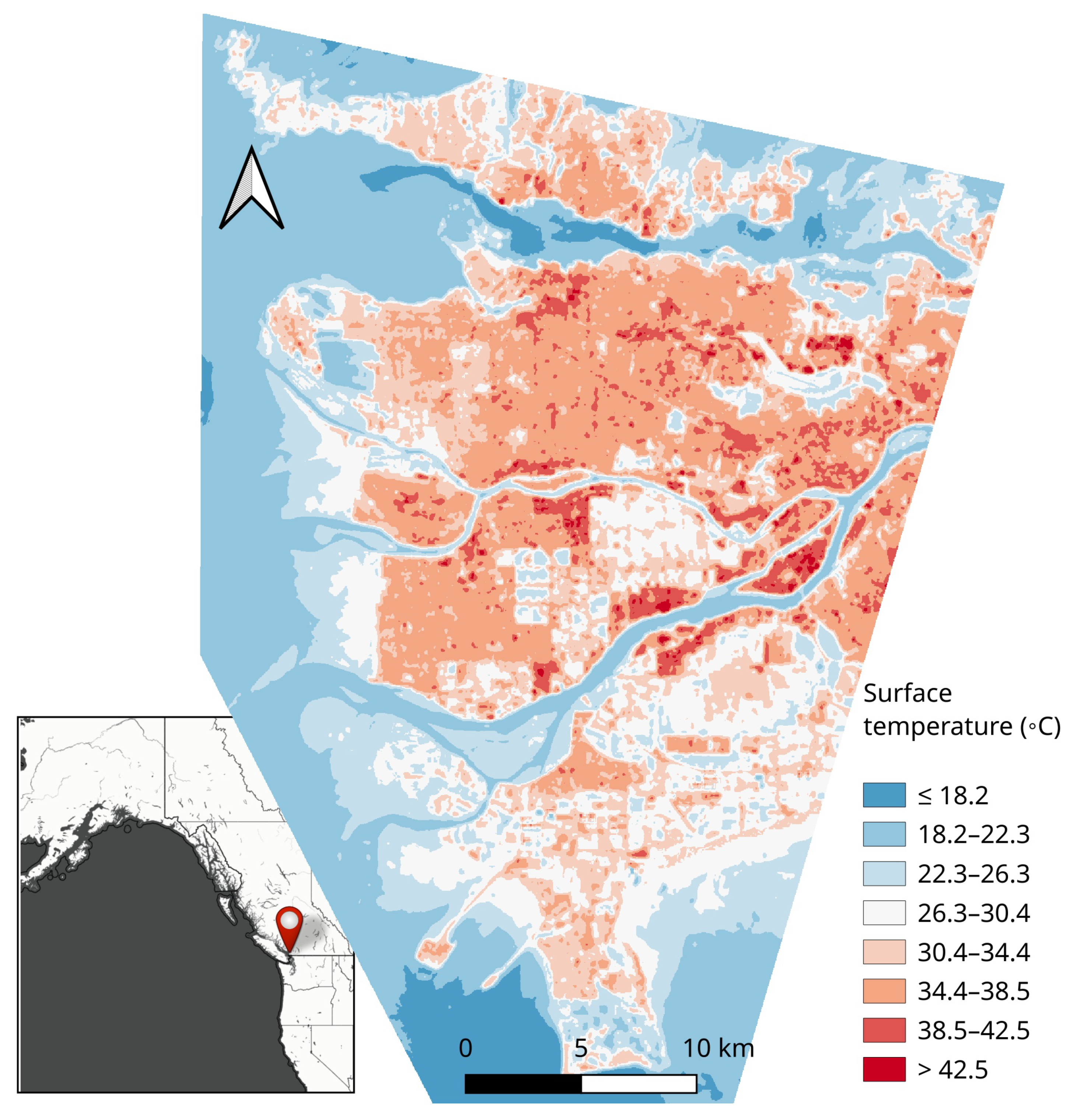
Metro Vancouver is a large metropolitan area (∼2.5 million residents) in the extreme southwest of Canada with warm wet winters and moderate dry summers. We selected a study region in Metro Vancouver such that it was covered by a single Landsat image, near sea level, and urban or peri-urban (see Figure 1). Most of the planted street trees in this region are non-native broadleaf deciduous trees [26], while native forests are dominated by conifers, including Douglas fir (Pseudotsuga menziesii), western hemlock (Tsuga heterophylla), and western red cedar (Thuja plicata) with some broadleaf trees, including red alder (Alnus rubra) and bigleaf maple (Acer macrophyllum) [27]. The first author has spent five years as a settler in the Vancouver, BC, and his first-hand experiences of how air temperature varied across different arboreal habitats motivated the conceptualization of this study.
2.2. Data
2.2.1. Land Cover Classification
We used the Land Cover Classification 2014–5 m Hybrid (Raster; updated in November 2019) dataset from http://www.metrovancouver.org/data (accessed on 26 January 2021) (see Figure 2). This dataset was created by Metro Vancouver using RapidEye 5 m multi-spectral satellite imagery and LiDAR (the latter was only available in the city of Vancouver). This dataset is only available in a format accessible by ArcGIS, so we used ArcGIS to export the raster as a TIF for processing in QGIS. We split the categorical raster into multiple binary rasters, one for each of the following 11 land cover classes: buildings (buildings), other built structures (otherBuilt), paved surfaces (paved), barren ground (barren), exposed soil (soil), coniferous trees (coniferous), deciduous trees (deciduous), shrubs of any type (shrubs), modified grass and herb, including lawns (modifiedGrassHerb), less modified grass and herb, including fields (naturalGrassHerb), and non-photosynthetic vegetation, including dead grass (nonPhotoVeg) (see Figure 2). We combined the remaining bands (no data, shadow, clouds/ice, and water) into an ’other’ binary raster to verify full coverage of the dataset, but not for use in the analysis.
2.2.2. Landsat
We used Landsat 8 to estimate surface temperature, albedo, and surface water. We downloaded Landsat 8 images (collection 2, level 2; [28]) for 3 August 2019 (USGS number: LC08_L2SP_048026_20190803_20200827_02_T1) from https://earthexplorer.usgs.gov/ (accessed on 26 January 2021). The surface temperature band accounts for variable emissivity (estimated from ASTER GED) and makes other corrections [29]. We selected an image from Summer 2019 so that it would be contemporaneous with the land cover dataset. We chose an image taken on 3 August because, on average, 1 August is the hottest day of the year (https://weatherspark.com/m/476/8/Average-Weather-in-August-in-Vancouver-Canada (accessed on 22 January 2021). Early August images will therefore capture the features relevant for understanding the highest temperatures in Vancouver. The image was taken at 19:07 UTC (12:07 p.m. PDT), so it captures the peak sun exposure. The image is cloud free over our study area and exhibits a 30 m resolution (see Figure 2).
Band Transformations
To convert the surface temperature band to Kelvin, we multiplied by 0.00341802 and added 149.0, as described in the Data Format Control Book [29], and then converted to Celsius (see Figure 1). Similarly, for bands 1 through 7, we multiplied each by 2.75 × 10⁻⁵ and subtracted 0.2 to convert the calibrated reflectance bands into radiance units (measured in W/(m2 sr um). We also estimated albedo because albedo is often a key driver of microclimate [30]. We calculated albedo using Equation (1), following Lee et al. [31].
To estimate the locations of surface water, we calculated the Modified Normalized Difference Water Index (MNDWI; [32]) using the following equation:
where MNDWI > 0 implies the presence of surface water, green is Landsat 8 band 3 (which is ∼TM band 2), and middle infrared (MIR) is Landsat 8 band 6 (which is ∼TM band 5). We visualized the resulting raster and validated it against high-resolution satellite data and known water sources. We found a very good mapping, and that it even correctly detected small swimming pools.
2.3. Spatial Analysis
We created a mask to define our area of interest (see Figure 1), cropped the surface temperature raster to this mask, then converted the new cropped raster to polygons (i.e., each landsat pixel became a polygon). To spatially join the albedo, land cover class, and MNDWI with surface temperature, we used zonal statistics. This produced a dataset that associated the albedo, surface temperature, MNDWI, and the number of enclosed pixels of each land cover class. All spatial processing was carried out using the PyQGIS interface to QGIS version 3.22, QGIS Development Team.
2.4. Air Temperature Comparison
To preliminarily understand the differences between Landsat surface temperature and in situ air temperature observations, we extracted the daily high air temperatures from two weather stations on Weather Underground (wunderground.com, accessed on 22 March 2021) for the same day as the Landsat observations.
2.5. Bayesian Models
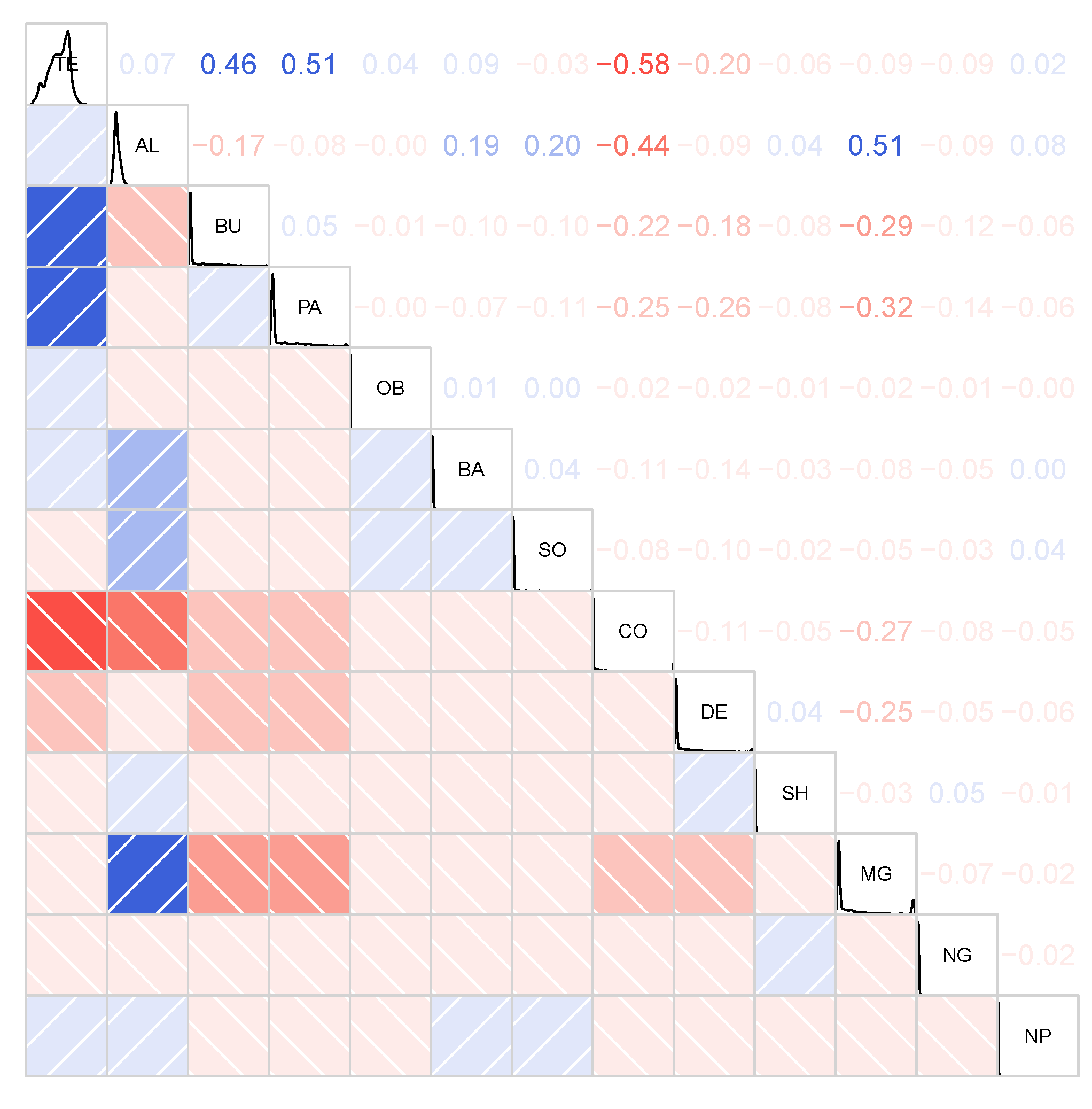
We first removed all locations with MNDWI > 0 (i.e., those that were surface water). Next, we checked that all of the land cover pixels (including the ‘other’ land cover) summed to 36 within each surface temperature polygon—we found this to be true for 99.7% of the polygons. After removing the ’other’ land covers (because there are very few of them and we hypothesized that these classes would not be informative for understanding surface temperature), we excluded all polygons from further analysis that summed to less than 0.5 × 36 = 18. For the remaining polygons, we normalized all of the land cover class values such that they summed to unity within each polygon. This produced a dataset with 791,902 polygons for further analysis. To understand the degree of collinearity between predictor variables (albedo and proportion of each land cover class), we calculated the correlations matrix of all variables (see Figure A1). To ease computation and clarify interaction effects, we standardized albedo such that it had a standard deviation of 0.5 and a mean of 0 [33].
Because the sum of all land cover class proportions is unity, including all land cover classes in a standard intercept–slope regression model produces redundancy (i.e. it is not full rank) [34,35]. To remove this redundancy, we adopted the Scheffe parametrization for mixture experiments, wherein the intercept is omitted and each dependent variable’s coefficient is interpreted as the value of the response variable if the mixture were entirely made up of that particular dependent variable [34]. In contrast, albedo did not share this dependency with the land cover classes, and so we treated it as a ‘process variable’ and included only the interaction effects [36] between it and each land cover class. Our model for surface temperature therefore took the form:
where is the surface temperature variable, are the land cover class variables, are the first-order coefficients, is the standardized albedo variable, are the second-order interaction coefficients, and represents the number of land cover classes, and is the normally distributed random error.
Due to the high collinearity between albedo and some of the land cover classes (Figure A1), we also built a secondary model that excluded albedo:
To understand the effect of albedo alone on surface temperature, we built another secondary model of albedo on surface temperature, where is the intercept coefficient and is the slope coefficient:
Finally, we built another secondary model that used land cover class to predict albedo, following the same form as that in Equation (4), but with the non-standardized albedo replacing surface temperature as the response variable:
All models were fit using the Rstan (version 2.26.1) interface to Stan [37] with rstanarm (version 2.21.1) in R (version 4.1.2). Models were estimated using 4 chains, each with 2000 iterations (with the first half used for warmup and then discarded), and wide proper priors. Chain convergence was confirmed using [38]. We reported 95% credible intervals (CrI).
3. Results
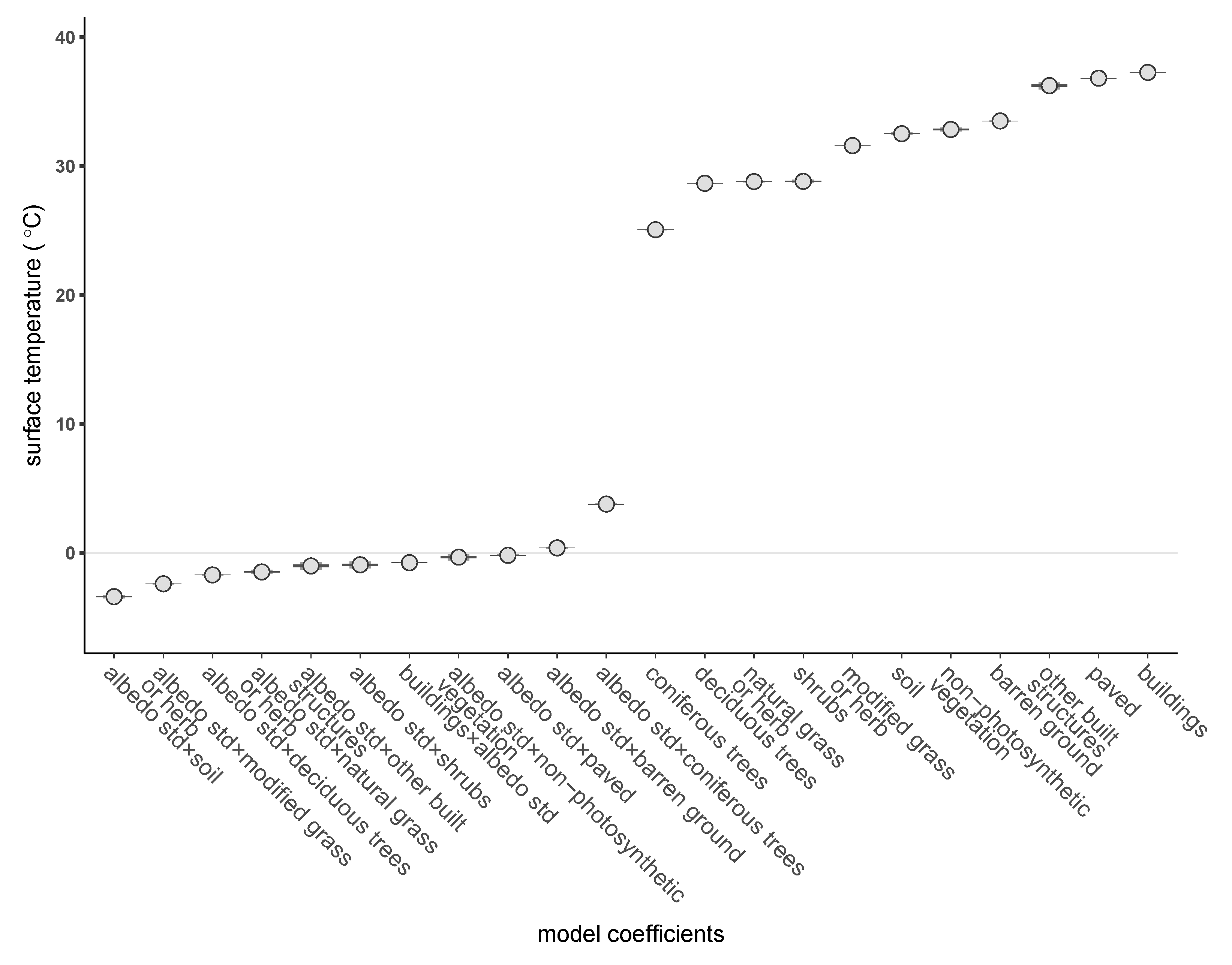
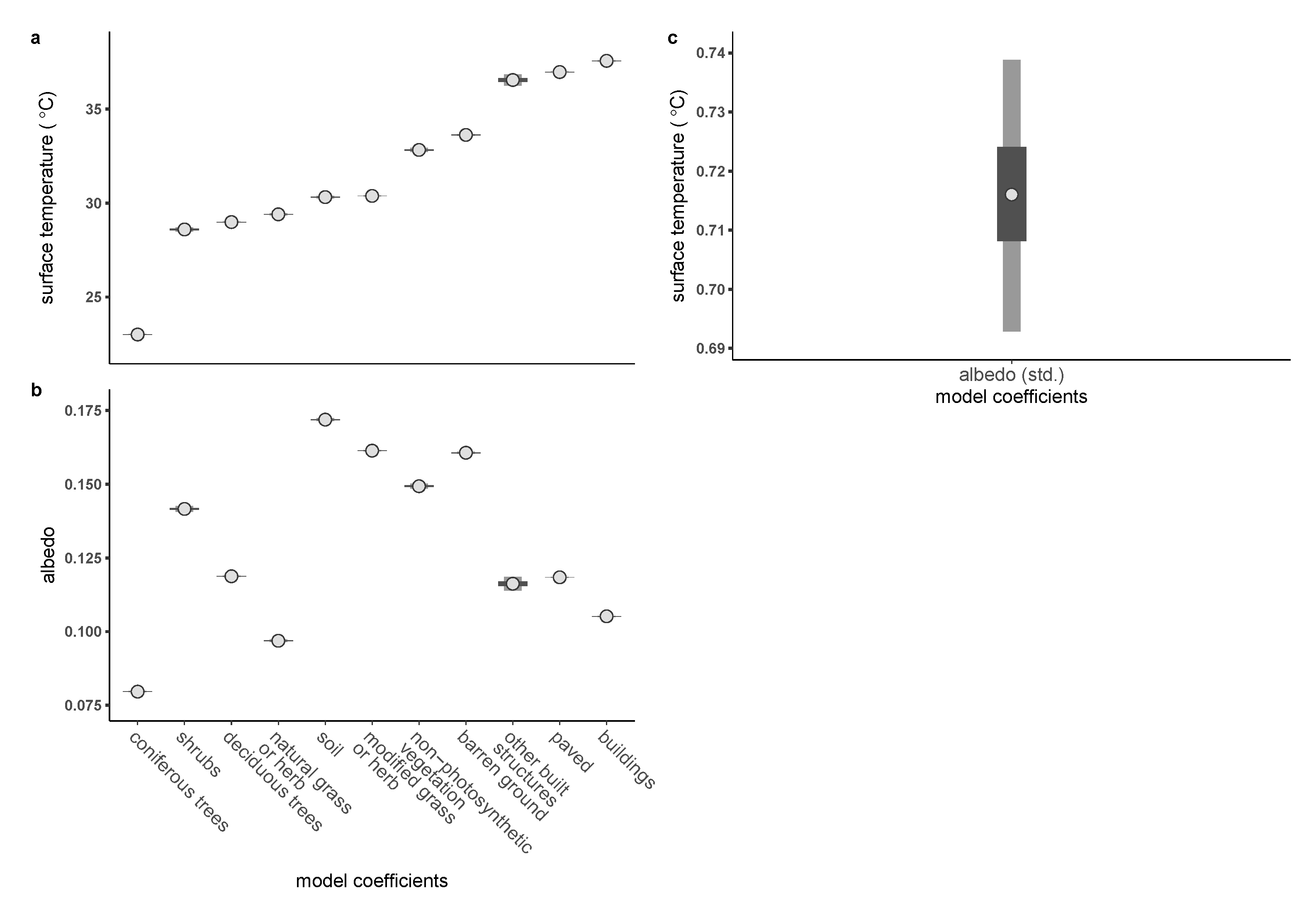
The mean surface temperature across the study area was 31.8 °C. Surface temperature varied significantly by land cover class. Surface temperature was highest at buildings (95% CrI: 37.24–37.29 °C), other built structures, and pavement, moderate at non-photosynthetic vegetation and barren ground, low at grass/herbs, bare soil, shrubs, and broadleaf deciduous trees (95% CrI: 28.65–28.69 °C ), and extremely low—more than 10 °C below buildings—at coniferous trees (95% CrI: 25.07–25.13 °C) (Figure 3, Table A1). The model without albedo (and thus without any challenges associated with collinearity) showed qualitatively similar results, though with some small shifts in estimates, including slightly larger differences between conifers and other cover classes (see Figure 4a).
The mean albedo across the study area was 0.12 and varied significantly by land cover class. Albedo was highest on bare soil (95% CrI: 0.17–0.17), and lowest on coniferous trees (95% CrI 0.08–0.08) (Figure 3, Table A3). Albedo values two standard deviations above the mean were associated with higher temperatures (95% CrI 0.69–0.74 °C).
For nearly all land cover classes, higher albedo within that class was associated with cooler temperatures (interaction terms in Figure 3). However, higher albedo was associated with an increase in conifer surface temperature (95% CrI 3.71–3.88 °C).
Landsat surface temperature and nearby in situ air temperature readings exhibited a positive correlation, although the surface temperature was higher (Landsat surface temperature = 30.1 and 35.7 °C; Weather Underground air temperature = 24.6 and 25.8 °C, respectively).
4. Discussion
This study leveraged remote sensing surface temperature data and high-resolution land cover data to investigate the capacity for coniferous and broadleaf trees to ameliorate high summer temperatures in the Pacific Northwest. While broadleaf trees and other vegetation were associated with cooler surface temperatures than buildings and pavement, we found that conifers were substantially cooler even than broadleaf trees, suggesting that conifers may be most effective in ameliorating urban heat waves in the Pacific Northwest of North America. The high degree of cooling associated with conifers is an encouraging result for cities as they adapt to climate change and the threat of more severe heat waves. Nevertheless, cooling capacity is only one of a suite of factors that should be considered when deciding how to afforest cities.
The large effect of tree type is consistent with previous studies [19], but ours is one of the first to show the effect of conifers. The mechanisms driving this effect may be related to tree form, structure [39], and leaf anatomy: Rahman et al. [19] found that needle-bearing trees exhibited higher shading capacity than other trees. The effect could also be due to differential evapotranspiration rates. Ewers et al. [40] found that white cedar (Thuja occidentalis)—a congener of one of the dominant conifers in our study—exhibited the highest hydraulic conductivity of the trees in their study, which is related to evapotranspiration rates. Hydraulic conductivity is usually higher in species adapted to wet soils. Because the conifers in our study area are mostly native, while the broadleaf trees are mostly not, it is possible that the conifers are better adapted to the wet temperate rainforest conditions and thus transpire faster than the non-native planted broadleaf trees. More research is needed on the mechanisms that drive conifer cooling.
The positive interaction effect between conifers and albedo (Figure 3) further suggests that evapotranspiration may be a key cooling mechanism for conifers. Studies often assume that surface temperature is negatively associated with albedo, except over water [30]. However, our results suggest that conifers with a lower albedo were actually cooler. Furthermore, evapotranspiration rates often vary inversely with albedo [41]. Therefore, it seems likely that lower albedo in conifers leads to higher evapotranspiration rates and thus lower temperatures. Because broadleaf deciduous trees showed the opposite relationship with albedo and temperature, evapotranspiration may play a larger role in cooling conifers than broadleaf trees. Moreover, these differential results suggest that land cover type—beyond surface water—is an important mediator of the albedo–temperature relationship.
Previous studies have shown that transpiration was higher in trees planted in grass than those planted in paved cutouts [19]. Broadleaf trees are more prevalent along Vancouver’s streets due to their root morphology [42] and the aesthetic preferences of Vancouver’s mostly British colonizers [43]. Thus, it is possible that abundance of broadleaf trees near concrete sidewalks and paved roads may have contributed to the higher temperature of broadleaf trees in our study. However, Pace et al. [44] found that water availability and wind speed were more important for determining transpiration rates than ground surface. Future research might assess how planting substrate mediates the relationship between tree type and surface temperature in Vancouver.
Surface temperatures are easy to quantify using remote sensing and correlate with air temperature [45]. However, the complexity of urban environments can complicate this relationship via microscale advection [46]. Thus, future work might measure air temperature in situ and assess how air temperature and surface temperature differ across land cover classes (beyond the very preliminary comparison that we conducted).
Our study focused on the differences between coniferous vs. broadleaf trees because these data exist at the metro-scale. The strong effect observed suggests that tree species is an important factor in determining surface temperature. Greater resolution in tree type may therefore be warranted. As hyperspectral imaging and LiDAR methods improve, it may become possible to identify tree genus at the metro-scale [47,48]. Including tree genus in surface temperature models could demonstrate to city planners what tree genera to plant in order to ameliorate heat waves.
Our findings may not generalize to other times of day. We chose to analyze urban surface temperatures at noon when they are likely to be most severe. However, studies have shown that cooling effects of trees and lawns may reverse at night, since trees retain moisture and disrupt cooling airflow over the ground [25]. Furthermore, urban heat island effects are most severe at night [9]. Future studies might examine how surface temperature–conifer relationships vary over the course of the day. Future work might also analyze the spatial arrangement and clustering of land cover classes (perhaps across similar urban and rural landscapes), which may affect surface temperatures [49].
Local and global climates are interconnected. In addition to regulating the local climate, afforestation and abatement of deforestation could also help regulate global climate. For example, urban tree planting is part of Canada’s Natural Climate Solutions Fund 2 Billion Trees Program, which aims to plant trees to uptake 2–4 megatons of CO2 per year by 2030 [50]. Such programs might help regulate local temperatures too if they target trees with higher cooling capacity, such as conifers.
However, global climate change may reduce the effectiveness of native conifers as a heat wave mitigation strategy. Rising temperatures may reduce growth of native conifers in this region: for example, Restaino et al. [51] showed that Douglas fir (Pseudotsuga menziesii)—a dominant conifer in the Pacific Northwest—is predicted to grow significantly slower in the face of climate change. Nevertheless, there are other co-benefits to planting native conifers as a climate mitigation strategy, including for birds, insects, and people [52,53,54]. Local afforestation may help ameliorate some of the effects of climate change, but in order to be most effective, it must be tied to simultaneous and aggressive efforts to curtail global climate change.
Author Contributions
Conceptualization, B.B. and H.N.E.; analysis, H.N.E. with assistance from B.B.; writing—original draft preparation, H.N.E.; writing—review and editing, H.N.E. and B.B.; visualization, H.N.E., with assistance from B.B.; project administration, H.N.E. and B.B.; funding acquisition, H.N.E. and B.B. All authors have read and agreed to the published version of the manuscript.
Funding
This research was funded by a Gund Postdoctoral Fellowship to HNE and by Environment and Climate Change Canada (GCXE22S079).
Institutional Review Board Statement
Not applicable.
Informed Consent Statement
Not applicable.
Data Availability Statement
This paper does not contain any original data. All custom code has been archived with the Open Science Foundation: http://0-doi-org.brum.beds.ac.uk/10.17605/OSF.IO/WVB7U, accessed on 20 March 2022.
Acknowledgments
We thank RS Delima and R Moran for feedback on figure design and E Ziglar for administrative support. We acknowledge that this work was carried out on land which has long served as a site of meeting and exchange among indigenous peoples and is home of the Abenaki People.
Conflicts of Interest
The authors declare no conflict of interest. The funders had no role in the design of the study; in the collection, analyses, or interpretation of data; in the writing of the manuscript, or in the decision to publish the results.
Appendix A
Figure A1.
Correlation and density plots for each variable used in our analysis. Blue signifies a positive correlation, while red signifies a negative correlation. Fainter colored boxes and text signify a weaker correlation. TE = surface temperature, AL = albedo, BU=buildings, PA = paved, OB = other built structures, BA = barren ground, SO = soil, CO = coniferous trees, DE = deciduous trees, SH = shrubs, MG = modified grass or herb, NG = natural grass or herb, NP = non-photosynthetic vegetation.


Table A1.
Summary of model of effects of land cover class and albedo on surface temperature.
| Mean | SD | 2.5% | 50% | 97.5% | n_eff | Rhat | |
|---|---|---|---|---|---|---|---|
| buildings | 37.27 | 0.01 | 37.24 | 37.27 | 37.29 | 5520.00 | 1.00 |
| paved | 36.82 | 0.01 | 36.80 | 36.82 | 36.84 | 6138.00 | 1.00 |
| otherBuilt | 36.25 | 0.14 | 35.97 | 36.25 | 36.52 | 7381.00 | 1.00 |
| barren | 33.50 | 0.03 | 33.45 | 33.51 | 33.56 | 5216.00 | 1.00 |
| soil | 32.52 | 0.05 | 32.43 | 32.52 | 32.61 | 2293.00 | 1.00 |
| coniferous | 25.07 | 0.03 | 25.02 | 25.07 | 25.13 | 1331.00 | 1.00 |
| deciduous | 28.67 | 0.01 | 28.65 | 28.67 | 28.69 | 6124.00 | 1.00 |
| shrubs | 28.82 | 0.06 | 28.70 | 28.82 | 28.94 | 7278.00 | 1.00 |
| modifiedGrassHerb | 31.59 | 0.01 | 31.57 | 31.59 | 31.62 | 3230.00 | 1.00 |
| naturalGrassHerb | 28.81 | 0.03 | 28.74 | 28.81 | 28.87 | 4271.00 | 1.00 |
| nonPhotoVeg | 32.85 | 0.07 | 32.71 | 32.85 | 32.98 | 3722.00 | 1.00 |
| buildings × albedo_std | −0.75 | 0.02 | −0.79 | −0.75 | −0.71 | 7190.00 | 1.00 |
| albedo_std × paved | −0.18 | 0.03 | −0.24 | −0.18 | −0.12 | 7399.00 | 1.00 |
| albedo_std × otherBuilt | −1.00 | 0.16 | −1.32 | −1.00 | −0.69 | 7191.00 | 1.00 |
| albedo_std × barren | 0.39 | 0.04 | 0.31 | 0.39 | 0.47 | 5799.00 | 1.00 |
| albedo_std × soil | −3.39 | 0.06 | −3.51 | −3.39 | −3.28 | 2357.00 | 1.00 |
| albedo_std × coniferous | 3.79 | 0.04 | 3.71 | 3.79 | 3.88 | 1354.00 | 1.00 |
| albedo_std × deciduous | −1.70 | 0.03 | −1.77 | −1.70 | −1.63 | 8035.00 | 1.00 |
| albedo_std × shrubs | −0.92 | 0.13 | −1.19 | −0.92 | −0.66 | 6588.00 | 1.00 |
| albedo_std × modifiedGrassHerb | −2.39 | 0.02 | −2.43 | −2.39 | −2.35 | 3121.00 | 1.00 |
| albedo_std × naturalGrassHerb | −1.47 | 0.08 | −1.62 | −1.47 | −1.32 | 4419.00 | 1.00 |
| albedo_std × nonPhotoVeg | −0.33 | 0.13 | −0.57 | −0.33 | −0.08 | 3788.00 | 1.00 |
| sigma | 3.15 | 0.00 | 3.14 | 3.15 | 3.15 | 1555.00 | 1.00 |
Table A2.
Summary of model on effects of land cover class on surface temperature.
| mean | sd | 2.5% | 50% | 97.5% | n_eff | Rhat | |
|---|---|---|---|---|---|---|---|
| buildings | 37.56 | 0.01 | 37.54 | 37.57 | 37.59 | 5618.00 | 1.00 |
| paved | 36.97 | 0.01 | 36.95 | 36.97 | 36.99 | 6143.00 | 1.00 |
| otherBuilt | 36.55 | 0.15 | 36.25 | 36.55 | 36.83 | 5412.00 | 1.00 |
| barren | 33.62 | 0.03 | 33.57 | 33.62 | 33.67 | 4992.00 | 1.00 |
| soil | 30.32 | 0.03 | 30.26 | 30.32 | 30.38 | 4876.00 | 1.00 |
| coniferous | 23.01 | 0.01 | 22.98 | 23.01 | 23.03 | 6251.00 | 1.00 |
| deciduous | 28.99 | 0.01 | 28.97 | 28.99 | 29.01 | 5824.00 | 1.00 |
| shrubs | 28.59 | 0.06 | 28.48 | 28.60 | 28.71 | 5181.00 | 1.00 |
| modifiedGrassHerb | 30.38 | 0.01 | 30.36 | 30.38 | 30.40 | 7429.00 | 1.00 |
| naturalGrassHerb | 29.40 | 0.03 | 29.35 | 29.40 | 29.45 | 4701.00 | 1.00 |
| nonPhotoVeg | 32.82 | 0.05 | 32.72 | 32.83 | 32.93 | 4411.00 | 1.00 |
| sigma | 3.21 | 0.00 | 3.20 | 3.21 | 3.21 | 683.00 | 1.00 |
Table A3.
Summary of model on effects of land cover class on on albedo.
| Mean | SD | 2.5% | 50% | 97.5% | n_eff | Rhat | |
|---|---|---|---|---|---|---|---|
| buildings | 0.11 | 0.00 | 0.10 | 0.11 | 0.11 | 5745.00 | 1.00 |
| paved | 0.12 | 0.00 | 0.12 | 0.12 | 0.12 | 5303.00 | 1.00 |
| otherBuilt | 0.12 | 0.00 | 0.11 | 0.12 | 0.12 | 4810.00 | 1.00 |
| barren | 0.16 | 0.00 | 0.16 | 0.16 | 0.16 | 4966.00 | 1.00 |
| soil | 0.17 | 0.00 | 0.17 | 0.17 | 0.17 | 4654.00 | 1.00 |
| coniferous | 0.08 | 0.00 | 0.08 | 0.08 | 0.08 | 5753.00 | 1.00 |
| deciduous | 0.12 | 0.00 | 0.12 | 0.12 | 0.12 | 5485.00 | 1.00 |
| shrubs | 0.14 | 0.00 | 0.14 | 0.14 | 0.14 | 3948.00 | 1.00 |
| modifiedGrassHerb | 0.16 | 0.00 | 0.16 | 0.16 | 0.16 | 6186.00 | 1.00 |
| naturalGrassHerb | 0.10 | 0.00 | 0.10 | 0.10 | 0.10 | 4127.00 | 1.00 |
| nonPhotoVeg | 0.15 | 0.00 | 0.15 | 0.15 | 0.15 | 4629.00 | 1.00 |
| sigma | 0.03 | 0.00 | 0.03 | 0.03 | 0.03 | 1188.00 | 1.00 |
Table A4.
Summary of model on effects of standardized albedo on surface temperature.
| Mean | SD | 2.5% | 50% | 97.5% | n_eff | Rhat | |
|---|---|---|---|---|---|---|---|
| (Intercept) | 31.80 | 0.01 | 31.79 | 31.80 | 31.81 | 638.00 | 1.01 |
| albedo_std | 0.72 | 0.01 | 0.69 | 0.72 | 0.74 | 4452.00 | 1.00 |
| sigma | 5.16 | 0.00 | 5.16 | 5.16 | 5.17 | 2912.00 | 1.00 |
References
- Fischer, E.M.; Knutti, R. Anthropogenic contribution to global occurrence of heavy-precipitation and high-temperature extremes. Nat. Clim. Chang. 2015, 5, 560–564. [Google Scholar] [CrossRef]
- Mitchell, D.; Heaviside, C.; Vardoulakis, S.; Huntingford, C.; Masato, G.; Guillod, B.P.; Frumhoff, P.; Bowery, A.; Wallom, D.; Allen, M. Attributing human mortality during extreme heat waves to anthropogenic climate change. Environ. Res. Lett. 2016, 11, 074006. [Google Scholar] [CrossRef]
- Revich, B.A.; Shaposhnikov, D.A. Climate change, heat waves, and cold spells as risk factors for increased mortality in some regions of Russia. Stud. Russ. Econ. Dev. 2012, 23, 195–207. [Google Scholar] [CrossRef]
- Ministry of Public Safety & Solicitor General. BC Coroners Service (BCCS) Heat-Related Deaths–Knowledge Update 2021. Available online: https://www2.gov.bc.ca/assets/gov/birth-adoption-death-marriage-and-divorce/deaths/coroners-service/statistical/heat_related_deaths_in_bc_knowledge_update.pdf (accessed on 20 March 2022).
- Tait, C.; Hager, J.K.M.; First Nations in British Columbia threaten to block rail traffic over fire recovery fears. Globe Mail, 5 July 2021. Available online: https://www.theglobeandmail.com/canada/article-first-nations-in-british-columbia-threaten-to-block-rail-traffic-over/ (accessed on 20 March 2022).
- Watts, N.; Adger, W.N.; Agnolucci, P.; Blackstock, J.; Byass, P.; Cai, W.; Chaytor, S.; Colbourn, T.; Collins, M.; Cooper, A.; et al. Health and climate change: Policy responses to protect public health. Lancet 2015, 386, 1861–1914. [Google Scholar] [CrossRef]
- Russo, S.; Dosio, A.; Graversen, R.G.; Sillmann, J.; Carrao, H.; Dunbar, M.B.; Singleton, A.; Montagna, P.; Barbola, P.; Vogt, J.V. Magnitude of extreme heat waves in present climate and their projection in a warming world. J. Geophys. Res. Atmos. 2014, 119, 12500–12512. [Google Scholar] [CrossRef] [Green Version]
- Molina, L.T.; Molina, M.J.; Slott, R.S.; Kolb, C.E.; Gbor, P.K.; Meng, F.; Singh, R.B.; Galvez, O.; Sloan, J.J.; Anderson, W.P.; et al. Air Quality in Selected Megacities. J. Air Waste Manag. Assoc. 2004, 54, 1–73. [Google Scholar] [CrossRef]
- Oke, T.; Maxwell, G. Urban heat island dynamics in Montreal and Vancouver. Atmos. Environ. 1975, 9, 191–200. [Google Scholar] [CrossRef]
- Peng, S.; Piao, S.; Ciais, P.; Friedlingstein, P.; Ottle, C.; Bréon, F.M.; Nan, H.; Zhou, L.; Myneni, R.B. Surface Urban Heat Island Across 419 Global Big Cities. Environ. Sci. Technol. 2011, 46, 696–703. [Google Scholar] [CrossRef]
- Kong, J.; Zhao, Y.; Carmeliet, J.; Lei, C. Urban heat island and its interaction with heatwaves: A review of studies on mesoscale. Sustainability 2021, 13, 10923. [Google Scholar] [CrossRef]
- Wang, C.; Wang, Z.H.; Wang, C.; Myint, S.W. Environmental cooling provided by urban trees under extreme heat and cold waves in U.S. cities. Remote Sens. Environ. 2019, 227, 28–43. [Google Scholar] [CrossRef]
- Bowler, D.E.; Buyung-Ali, L.; Knight, T.M.; Pullin, A.S. Urban greening to cool towns and cities: A systematic review of the empirical evidence. Landsc. Urban Plan. 2010, 97, 147–155. [Google Scholar] [CrossRef]
- Wang, C.; Wang, Z.H.; Yang, J. Cooling Effect of Urban Trees on the Built Environment of Contiguous United States. Earth’s Future 2018, 6, 1066–1081. [Google Scholar] [CrossRef] [Green Version]
- Liébard, A.; de Herde, A. Traité D’architecture et D’urbanisme Bioclimatiques: Concevoir, Édifier et Aménager Avec le Développement Durable; Paris Observ’ER: Paris, France, 2005. [Google Scholar]
- Georgi, N.J.; Zafiriadis, K. The impact of park trees on microclimate in urban areas. Urban Ecosyst. 2006, 9, 195–209. [Google Scholar] [CrossRef]
- Domke, G.M.; Oswalt, S.N.; Walters, B.F.; Morin, R.S. Tree planting has the potential to increase carbon sequestration capacity of forests in the United States. Proc. Natl. Acad. Sci. USA 2020, 117, 24649–24651. [Google Scholar] [CrossRef]
- Vancouver City Planning Commission. Climate Emergency: Extreme Heat and Air Quality Mitigation; Vancouver City Planning Commission: Vancouver, BC, Canada, 2021. [Google Scholar]
- Rahman, M.A.; Stratopoulos, L.M.; Moser-Reischl, A.; Zölch, T.; Häberle, K.H.; Rötzer, T.; Pretzsch, H.; Pauleit, S. Traits of trees for cooling urban heat islands: A meta-analysis. Build. Environ. 2020, 170, 106606. [Google Scholar] [CrossRef]
- Rahman, M.A.; Armson, D.; Ennos, A.R. A comparison of the growth and cooling effectiveness of five commonly planted urban tree species. Urban Ecosyst. 2014, 18, 371–389. [Google Scholar] [CrossRef]
- Georgi, J.N.; Dimitriou, D. The contribution of urban green spaces to the improvement of environment in cities: Case study of Chania, Greece. Build. Environ. 2010, 45, 1401–1414. [Google Scholar] [CrossRef] [Green Version]
- Konarska, J.; Uddling, J.; Holmer, B.; Lutz, M.; Lindberg, F.; Pleijel, H.; Thorsson, S. Transpiration of urban trees and its cooling effect in a high latitude city. Int. J. Biometeorol. 2015, 60, 159–172. [Google Scholar] [CrossRef]
- Napoli, M.; Massetti, L.; Brandani, G.; Petralli, M.; Orlandini, S. Modeling Tree Shade Effect on Urban Ground Surface Temperature. J. Environ. Qual. 2016, 45, 146–156. [Google Scholar] [CrossRef]
- Song, J.; Wang, Z.H. Diurnal changes in urban boundary layer environment induced by urban greening. Environ. Res. Lett. 2016, 11, 114018. [Google Scholar] [CrossRef] [Green Version]
- Spronken-Smith, R.A.; Oke, T.R. The thermal regime of urban parks in two cities with different summer climates. Int. J. Remote Sens. 1998, 19, 2085–2104. [Google Scholar] [CrossRef]
- City of Vancouve Open Data Portal. Street Trees. 2022. Available online: https://opendata.vancouver.ca/explore/dataset/street-trees/information/ (accessed on 20 March 2022).
- Diamond Head Consulting. District of North Vancouver Fromme Mountain Area Ecosystem Analysis; Citeseer: Princeton, NJ, USA, 2004; pp. 1–22. [Google Scholar]
- Earth Resources Observation And Science (EROS) Center. Collection-2 Landsat 8-9 OLI (Operational Land Imager) and TIRS (Thermal Infrared Sensor) Level-2 Science Products. 2013. Available online: https://www.usgs.gov/centers/eros/science/usgs-eros-archive-landsat-archives-landsat-8-9-olitirs-collection-2-level-2 (accessed on 20 March 2022). [CrossRef]
- EROS. Landsat 8-9Operational Land Imager (OLI)-Thermal Infrared Sensor (TIRS)Collection 2 Level 2 (L2) Data Format Control Book (DFCB); United States Geological Survey: Reston, VA, USA, 2020. [Google Scholar]
- Dare, R. A system dynamics model to facilitate the development of policy for urban heat island mitigation. Urban Sci. 2021, 5, 19. [Google Scholar] [CrossRef]
- Lee, D.; Seo, M.; Lee, K.; Choi, S.; Sung, N.; Kim, H.; Jin, D.; Kwon, C.; Huh, M.; Han, K. Landsat 8-based high resolution surface broadband albedo retrieval. Korean J. Remote Sens. 2016, 32, 741–746. [Google Scholar] [CrossRef] [Green Version]
- Xu, H. Modification of normalised difference water index (NDWI) to enhance open water features in remotely sensed imagery. Int. J. Remote Sens. 2006, 27, 3025–3033. [Google Scholar] [CrossRef]
- Gelman, A. Scaling regression inputs by dividing by two standard deviations. Stat. Med. 2008, 27, 2865–2873. [Google Scholar] [CrossRef]
- Lawson, J.; Willden, C. Mixture experiments in R using mixexp. J. Stat. Softw. 2016, 72, 1–20. [Google Scholar] [CrossRef] [Green Version]
- Scheffé, H. Experiments with mixtures. J. R. Stat. Soc. Ser. B 1958, 20, 344–360. [Google Scholar] [CrossRef]
- Anderson-Cook, C.M.; Goldfarb, H.B.; Borror, C.M.; Montgomery, D.C.; Canter, K.G.; Twist, J.N. Mixture and mixture-process variable experiments for pharmaceutical applications. Pharm. Stat. 2004, 3, 247–260. [Google Scholar] [CrossRef]
- Carpenter, B.; Gelman, A.; Hoffman, M.D.; Lee, D.; Goodrich, B.; Betancourt, M.; Brubaker, M.; Guo, J.; Li, P.; Riddell, A. Stan: A probabilistic programming language. J. Stat. Softw. 2017, 76, 1–32. [Google Scholar] [CrossRef] [Green Version]
- Vehtari, A.; Gelman, A.; Simpson, D.; Carpenter, B.; Bürkner, P.C. Rank-normalization, folding, and localization: An improved R-hat for assessing convergence of MCMC (with Discussion). Bayesian Anal. 2021, 16, 667–718. [Google Scholar] [CrossRef]
- Domingo, F.; van Gardingen, P.; Brenner, A. Leaf boundary layer conductance of two native species in southeast Spain. Agric. For. Meteorol. 1996, 81, 179–199. [Google Scholar] [CrossRef]
- Ewers, B.E.; Mackay, D.S.; Gower, S.T.; Ahl, D.E.; Burrows, S.N.; Samanta, S.S. Tree species effects on stand transpiration in northern Wisconsin. Water Resour. Res. 2002, 38, 8-1–8-11. [Google Scholar] [CrossRef]
- Seginer, I. The effect of albedo on the evapotranspiration rate. Agric. Meteorol. 1969, 6, 5–31. [Google Scholar] [CrossRef]
- Melles, S. Effects of Landscape and Local Habitat Features on Bird Communities: A Study of an Urban Gradient in Greater Vancouver. Ph.D. Thesis, University of British Columbia, Vancouver, BC, Canada, 2000. [Google Scholar]
- Ley, D. Between Europe and Asia: The case of the missing sequoias. Ecumene 1995, 2, 187–212. [Google Scholar] [CrossRef]
- Pace, R.; Fino, F.D.; Rahman, M.A.; Pauleit, S.; Nowak, D.J.; Grote, R. A single tree model to consistently simulate cooling, shading, and pollution uptake of urban trees. Int. J. Biometeorol. 2021, 65, 277–289. [Google Scholar] [CrossRef]
- Stoll, M.J.; Brazel, A.J. Surface-air temperature relationships in the urban environment of Phoenix, Arizona. Phys. Geogr. 1992, 13, 160–179. [Google Scholar] [CrossRef]
- Shiflett, S.A.; Liang, L.L.; Crum, S.M.; Feyisa, G.L.; Wang, J.; Jenerette, G.D. Variation in the urban vegetation, surface temperature, air temperature nexus. Sci. Total Environ. 2017, 579, 495–505. [Google Scholar] [CrossRef]
- Budei, B.C.; St-Onge, B.; Hopkinson, C.; Audet, F.A. Identifying the genus or species of individual trees using a three-wavelength airborne lidar system. Remote Sens. Environ. 2018, 204, 632–647. [Google Scholar] [CrossRef]
- Wang, K.; Wang, T.; Liu, X. A review: Individual tree species classification using integrated airborne LiDAR and optical imagery with a focus on the urban environment. Forests 2019, 10, 1. [Google Scholar] [CrossRef] [Green Version]
- Myint, S.W.; Zheng, B.; Talen, E.; Fan, C.; Kaplan, S.; Middel, A.; Smith, M.; Huang, H.-P.; Brazel, A. Does the spatial arrangement of urban landscape matter? examples of urban warming and cooling in phoenix and las vegas. Ecosyst. Health Sustain. 2015, 1, 1–15. [Google Scholar] [CrossRef]
- Environment and Climate Change Canada. Nature Smart Climate Solutions Fund; Environment and Climate Change Canada: Vancouver, BC, Canada, 2021.
- Restaino, C.M.; Peterson, D.L.; Littell, J. Increased water deficit decreases Douglas fir growth throughout western US forests. Proc. Natl. Acad. Sci. USA 2016, 113, 9557–9562. [Google Scholar] [CrossRef] [PubMed] [Green Version]
- Melles, S.; Glenn, S.; Martin, K. Urban bird diversity and landscape complexity: Species– environment associations along a multiscale habitat gradient. Conserv. Ecol. 2003, 7, 1–22. [Google Scholar] [CrossRef] [Green Version]
- Tallamy, D.W. Do alien plants reduce insect biomass? Conserv. Biol. 2004, 18, 1689–1692. [Google Scholar] [CrossRef]
- Zahn, M.J.; Palmer, M.I.; Turner, N.J. “Everything we do, it’s cedar”: First Nation and ecologically-based forester land management philosophies in coastal british columbia. J. Ethnobiol. 2018, 38, 314. [Google Scholar] [CrossRef]
Figure 1.
Map of the location of the study region (bottom left) and the bounds of the study region colored by the Landsat-derived surface temperature. Inset map © OpenStreetMap.org contributors.
Figure 1.
Map of the location of the study region (bottom left) and the bounds of the study region colored by the Landsat-derived surface temperature. Inset map © OpenStreetMap.org contributors.

Figure 2.
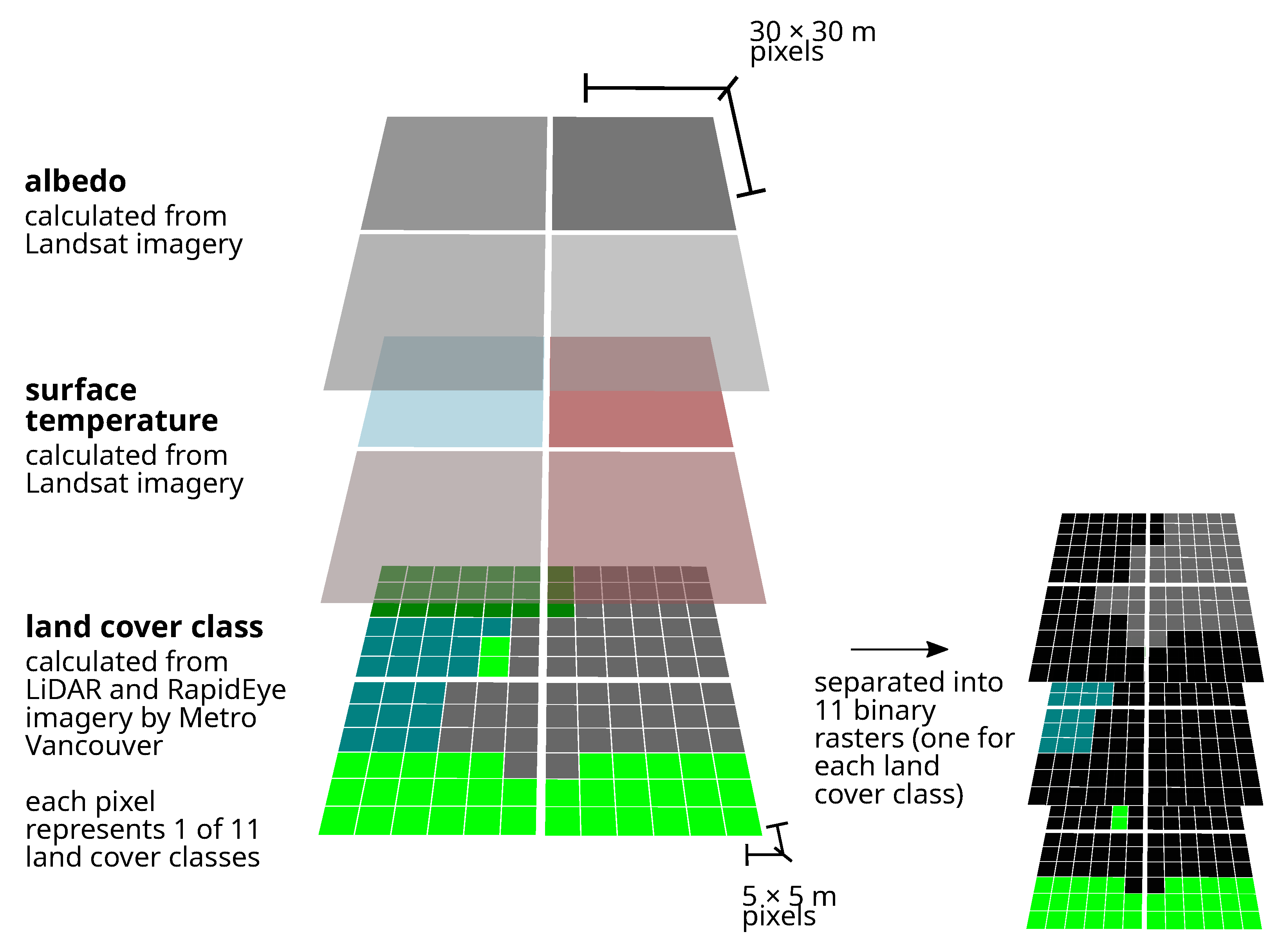
Diagram showing the three layers of data and spatial resolution of each. Albedo and surface temperature were derived from Landsat data and had pixel dimensions of 30 × 30 m. The land cover classes were taken from Metro Vancouver, and were ultimately derived from LiDAR data and RapidEye multispectral satellite imagery. Each land cover class pixel was 5 × 5 m. Thus, 36 land cover class pixels are together associated with a single surface temperature pixel. The land cover class raster was separated into 11 binary rasters for analysis (only 3 shown here for simplicity).
Figure 2.
Diagram showing the three layers of data and spatial resolution of each. Albedo and surface temperature were derived from Landsat data and had pixel dimensions of 30 × 30 m. The land cover classes were taken from Metro Vancouver, and were ultimately derived from LiDAR data and RapidEye multispectral satellite imagery. Each land cover class pixel was 5 × 5 m. Thus, 36 land cover class pixels are together associated with a single surface temperature pixel. The land cover class raster was separated into 11 binary rasters for analysis (only 3 shown here for simplicity).

Figure 3.
Main model results showing 95% credible intervals (outer) and 50% credible intervals (inner) of the effects of land cover classes (and their interactions with albedo) on surface temperature. See Table A1 for model coefficients. See Figure 4 for additional model results.

Figure 4.
Secondary model results showing 95% credible intervals (outer) and 50% credible intervals (inner) for the (a) model of the effects of land cover classes on surface temperature, (b) model of the effects of land cover classes on albedo, and (c) model of the effects of albedo on surface temperature. See Table A2–Table A4 for coefficient values.

Publisher’s Note: MDPI stays neutral with regard to jurisdictional claims in published maps and institutional affiliations. |
© 2022 by the authors. Licensee MDPI, Basel, Switzerland. This article is an open access article distributed under the terms and conditions of the Creative Commons Attribution (CC BY) license (https://creativecommons.org/licenses/by/4.0/).
Share and Cite
MDPI and ACS Style
Eyster, H.N.; Beckage, B. Conifers May Ameliorate Urban Heat Waves Better Than Broadleaf Trees: Evidence from Vancouver, Canada. Atmosphere 2022, 13, 830. https://0-doi-org.brum.beds.ac.uk/10.3390/atmos13050830
AMA Style
Eyster HN, Beckage B. Conifers May Ameliorate Urban Heat Waves Better Than Broadleaf Trees: Evidence from Vancouver, Canada. Atmosphere. 2022; 13(5):830. https://0-doi-org.brum.beds.ac.uk/10.3390/atmos13050830
Chicago/Turabian StyleEyster, Harold N., and Brian Beckage. 2022. "Conifers May Ameliorate Urban Heat Waves Better Than Broadleaf Trees: Evidence from Vancouver, Canada" Atmosphere 13, no. 5: 830. https://0-doi-org.brum.beds.ac.uk/10.3390/atmos13050830
Note that from the first issue of 2016, this journal uses article numbers instead of page numbers. See further details here.