
Response of Population Canopy Color Gradation Skewed Distribution Parameters of the RGB Model to Micrometeorology Environment in Begonia Fimbristipula Hance


Abstract
:1. Introduction
2. Materials and Methods
2.1. Plant Material and Growth Conditions
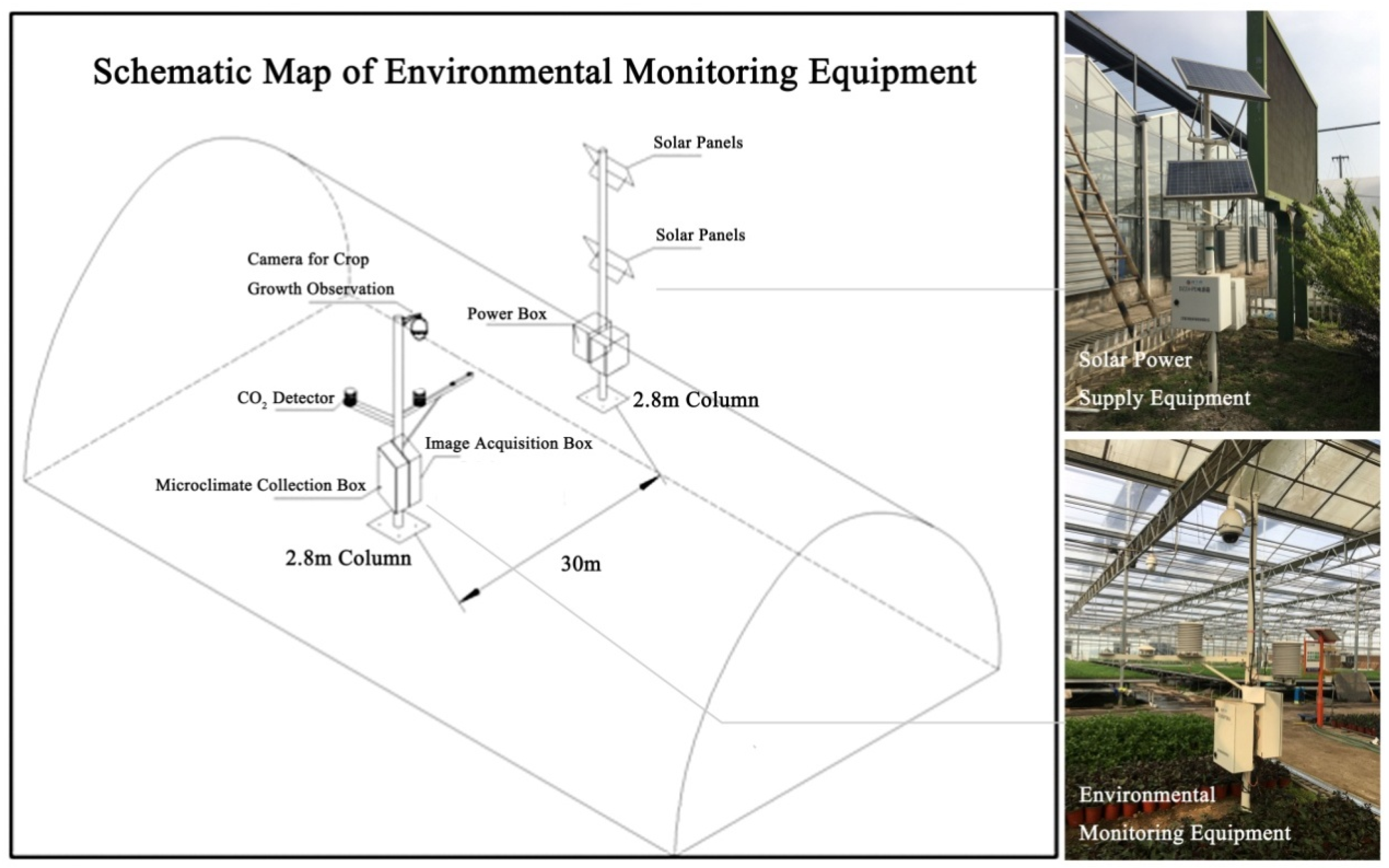
2.2. Meteorological Data Acquisition
2.3. Canopy Image Collection
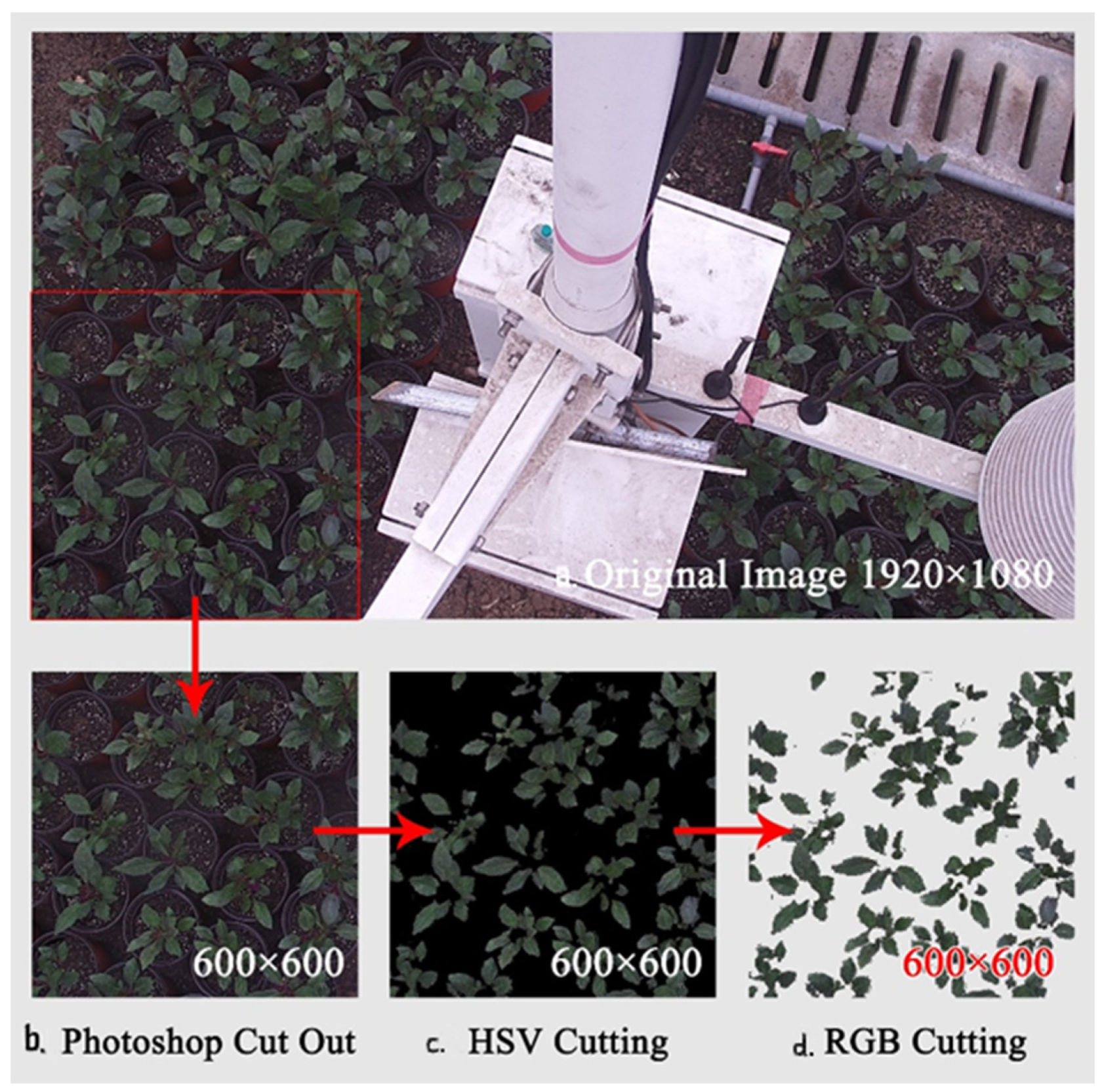
2.4. Cutting and Denoising of the Image
- Adobe Photoshop CS software (San Jose, CA, USA) was primarily used to intercept the range of 600 × 600 in the lower-left corner of the image, and the processed image was saved in a JPG image format (Figure 2b).
- The rgb2hsv function of MATLAB was used to convert RGB images into HSV images. Double cycle operation was used to set the H-value of the image background to 0 (i.e., black), while the H value of the plant remains unchanged. The hsv2rgb function was used to convert the processed HSV image into an RGB image (Figure 2c).
- The double cycle operation of MATLAB was used again to filter the color threshold value of the image processed in the previous step. The color opacity of the black part of the image was adjusted to 0 (that is, completely transparent), and the color image of the target leaf or canopy with the transparent background was saved as a PNG image mode (Figure 2d).
2.5. Information Collection of the RGB Image
2.6. Prediction Model Construction and Goodness-of-Fit Detection
3. Results
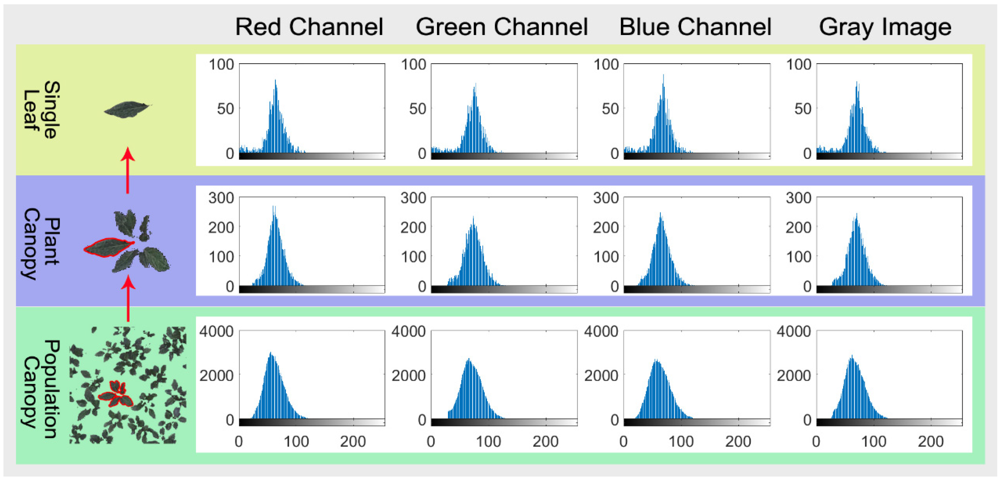
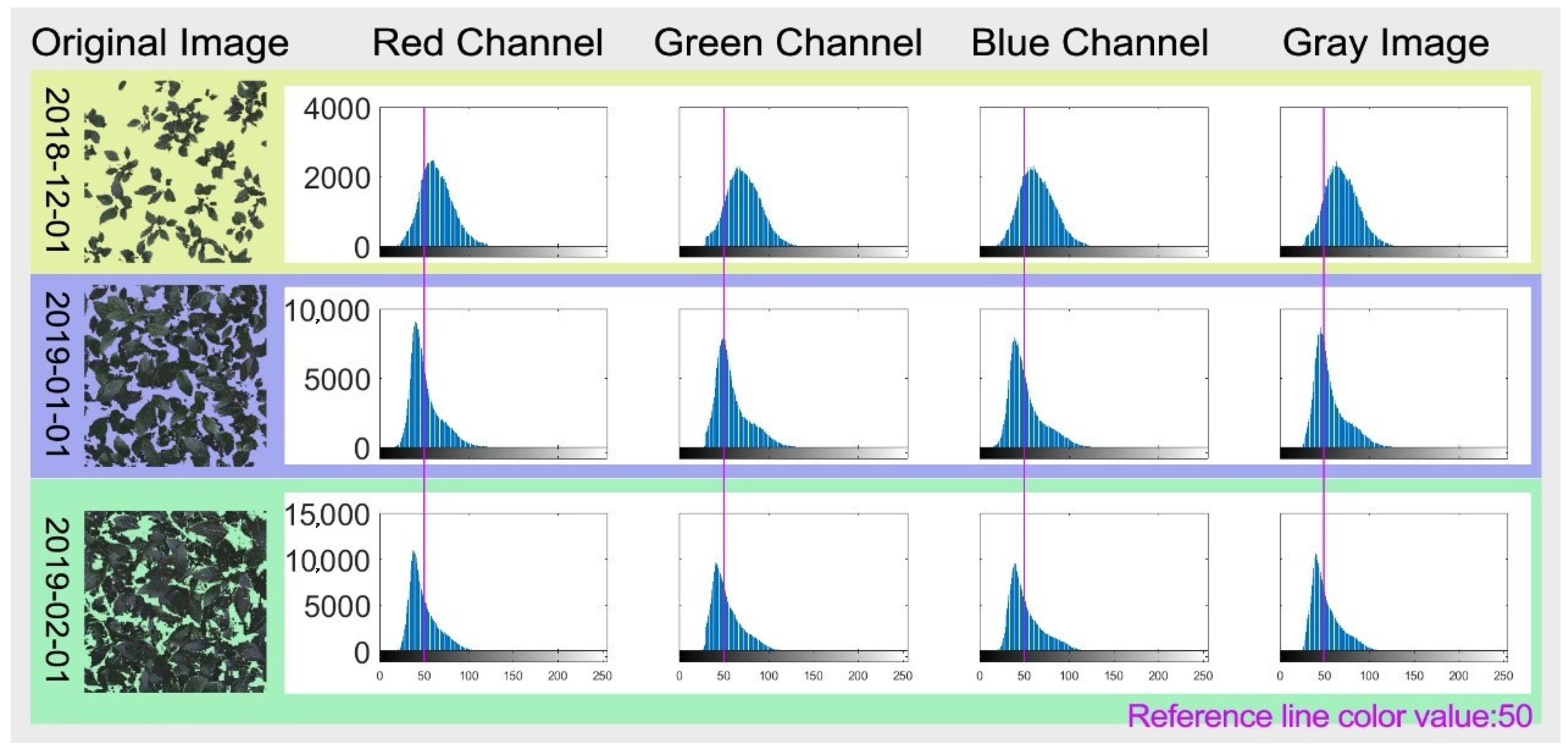
3.1. Skew Analysis of the Distribution of Leaf Color Gradation of the RGB Images
3.2. Correlation Analysis Microclimate Factors in Glasshouse and Population Canopy CGSD Parameters
3.3. Multiple Linear Relationships of the Microclimate Factors and Population Canopy CGSD Parameters
3.4. Optimization of Canopy Color Skewness-Meteorological Models
4. Discussion
5. Conclusions
Supplementary Materials
Author Contributions
Funding
Institutional Review Board Statement
Informed Consent Statement
Data Availability Statement
Conflicts of Interest
References
- Zhou, H.L.; Zhou, G.S.; He, Q.J.; Zhou, L.; Ji, Y.H.; Zhou, M.Z. Environmental explanation of maize specific leaf area under varying water stress regimes. Environ. Exp. Bot. 2019, 171, 103932. [Google Scholar] [CrossRef]
- Nawaz, R.; Abbasi, N.A.; Hafiz, I.A.; Khalid, A. Impact of climate variables on growth and development of Kinnow fruit (Citrus nobilis Lour x Citrus deliciosa Tenora) grown at different ecological zones under climate change scenario. Sci. Hortic. 2019, 260, 108868. [Google Scholar] [CrossRef]
- Kempkes, F.; De Zwart, H.; Muñoz, P.; Montero, J.; Baptista, F.; Giuffrida, F.; Gilli, C.; Stępowska, A.; Stanghellini, C. Heating and dehumidification in production greenhouses at northern latitudes: Energy use. Acta Hortic. 2017, 445–452. [Google Scholar] [CrossRef]
- Amani, M.; Foroushani, S.; Sultan, M.; Bahrami, M. Comprehensive review on dehumidification strategies for agricultural greenhouse applications. Appl. Therm. Eng. 2020, 181, 115979. [Google Scholar] [CrossRef]
- Guo, Y.; Zhao, H.; Zhang, S.; Wang, Y.; Chow, D. Modeling and optimization of environment in agricultural greenhouses for improving cleaner and sustainable crop production. J. Clean. Prod. 2020, 285, 124843. [Google Scholar] [CrossRef]
- Chen, D.; Neumann, K.; Friedel, S.; Kilian, B.; Chen, M.; Altmann, T.; Klukas, C. Dissecting the Phenotypic Components of Crop Plant Growth and Drought Responses Based on High-Throughput Image Analysis. Plant Cell 2014, 26, 4636–4655. [Google Scholar] [CrossRef] [Green Version]
- He, J.Q.; Harrison, R.J.; Li, B. A novel 3D imaging system for strawberry phenotyping. Plant Methods 2017, 13, 1–8. [Google Scholar] [CrossRef]
- Sancho-Adamson, M.; Trillas, M.I.; Bort, J.; Fernandez-Gallego, J.A.; Romanyà, J. Use of RGB Vegetation Indexes in Assessing Early Effects of Verticillium Wilt of Olive in Asymptomatic Plants in High and Low Fertility Scenarios. Remote Sens. 2019, 11, 607. [Google Scholar] [CrossRef] [Green Version]
- Liu, Z.; Hu, H.; Yu, H.; Yang, X.; Yang, H.; Ruan, C.; Wang, Y.; Tang, J. Relationship between leaf physiologic traits and canopy color indices during the leaf expansion period in an oak forest. Ecosphere 2015, 6, art259. [Google Scholar] [CrossRef]
- Grosskinsky, D.K.; Syaifullah, S.J.; Roitsch, T. Integration of multi-omics techniques and physiological phenotyping within a holistic phenomics approach to study senescence in model and crop plants. J. Exp. Bot. 2017, 69, 825–844. [Google Scholar] [CrossRef] [Green Version]
- Vasseur, F.; Bresson, J.; Wang, G.; Schwab, R.; Weigel, D. Image-based methods for phenotyping growth dynamics and fitness components in Arabidopsis thaliana. Plant Methods 2018, 14, 1–11. [Google Scholar] [CrossRef]
- Barker, J.; Zhang, N.Q.; Sharon, J.; Steeves, R.; Wang, X.; Wei, Y.; Poland, J. Development of a field-based high-throughput mobile phenotyping platform. Comput. Electron. Agric. 2016, 122, 74–85. [Google Scholar] [CrossRef] [Green Version]
- Dey, A.K.; Sharma, M.; Meshram, M. An Analysis of Leaf Chlorophyll Measurement Method Using Chlorophyll Meter and Image Processing Technique. Procedia Comput. Sci. 2016, 85, 286–292. [Google Scholar] [CrossRef] [Green Version]
- Yadav, S.P.; Ibaraki, Y.; Gupta, S.D. Estimation of the chlorophyll content of micropropagated potato plants using RGB based image analysis. Plant Cell Tissue Organ. Cult. (PCTOC) 2009, 100, 183–188. [Google Scholar] [CrossRef]
- Adamsen, F.J.; Pinter, P.J.; Barnes, E.M.; Lamorte, R.L.; Wall, G.W.; Leavitt, S.W.; Kimball, B.A. Measuring Wheat Senescence with a Digital Camera. Crop Sci. 1999, 39, 719–724. [Google Scholar] [CrossRef]
- Hu, H.; Liu, H.-Q.; Zhang, H.; Zhu, J.-H.; Yao, X.-G.; Zhang, X.-B.; Zheng, K.-F. Assessment of Chlorophyll Content Based on Image Color Analysis, Comparison with SPAD-502. In Proceedings of the 2nd International Conference on Information Engineering and Computer Science (ICIECS), Wuhan, China, 25–26 December 2010; pp. 476–478. [Google Scholar] [CrossRef]
- Ali, M.M.; Al-Ani, A.; Eamus, D.; Tan, D.K.Y.A. New image processing based technique to determine chlorophyll in plants. Am. Eurasian J. Agric. Environ. Sci. 2012, 12, 1323–1328. [Google Scholar] [CrossRef]
- Han, W.T.; Sun, Y.; Xu, T.F.; Chen, X.W.; Su, K.O. Detecting maize leaf water status by using digital RGB images. Int. J. Agric. Biol. Eng. 2014, 7, 45–53. [Google Scholar] [CrossRef]
- Barbedo, J.G.A. Detection of nutrition deficiencies in plants using proximal images and machine learning: A review. Comput. Electron. Agric. 2019, 162, 482–492. [Google Scholar] [CrossRef]
- Humplík, J.F.; Lazár, D.; Husičková, A.; Spíchal, L. Automated phenotyping of plant shoots using imaging methods for analysis of plant stress responses—A review. Plant Methods 2015, 11, 1–10. [Google Scholar] [CrossRef] [Green Version]
- Humplík, J.F.; Lazár, D.; Fürst, T.; Husičková, A.; Hýbl, M.; Spíchal, L. Automated integrative high-throughput phenotyping of plant shoots: A case study of the cold-tolerance of pea (Pisum sativum L.). Plant Methods 2015, 11, 20. [Google Scholar] [CrossRef] [Green Version]
- Bresson, J.; Bieker, S.; Riester, L.; Doll, J.; Zentgraf, U. A guideline for leaf senescence analyses: From quantification to physiological and molecular investigations. J. Exp. Bot. 2017, 69, 769–786. [Google Scholar] [CrossRef]
- Li, L.; Zhang, Q.; Huang, D. A Review of Imaging Techniques for Plant Phenotyping. Sensors 2014, 14, 20078–20111. [Google Scholar] [CrossRef]
- Neilson, E.H.; Edwards, A.M.; Blomstedt, C.K.; Berger, B.; Møller, B.L.; Gleadow, R.M. Utilization of a high-throughput shoot imaging system to examine the dynamic phenotypic responses of a C4 cereal crop plant to nitrogen and water deficiency over time. J. Exp. Bot. 2015, 66, 1817–1832. [Google Scholar] [CrossRef]
- Bai, G.; Jenkins, S.; Yuan, W.; Graef, G.L.; Ge, Y. Field-Based Scoring of Soybean Iron Deficiency Chlorosis Using RGB Imaging and Statistical Learning. Front. Plant Sci. 2018, 9, 1002–1011. [Google Scholar] [CrossRef] [Green Version]
- Gracia-Romero, A.; Kefauver, S.C.; Vergara-Díaz, O.; Zaman-Allah, M.; Prasanna, B.M.; Cairns, J.; Araus, J.L. Comparative Performance of Ground vs. Aerially Assessed RGB and Multispectral Indices for Early-Growth Evaluation of Maize Performance under Phosphorus Fertilization. Front. Plant Sci. 2017, 8, 2004. [Google Scholar] [CrossRef] [Green Version]
- Tester, M.; Langridge, P. Breeding Technologies to Increase Crop Production in a Changing World. Science 2010, 327, 818–822. [Google Scholar] [CrossRef]
- Bunce, J.A. Responses of stomatal conductance to light, humidity and temperature in winter wheat and barley grown at three concentrations of carbon dioxide in the field. Global Change Biol 2000, 6, 371–382. [Google Scholar] [CrossRef]
- Min-Wha, J.; Mohammad, B.A.; Eun-Joo, H.; Kee-Yoeup, P. Photosynthetic pigments, morphology and leaf gas exchange during ex vitro acclimatization of micropropagated CAM Doritaenopsis plantlets under relative humidity and air temperature. Environ. Exp. Bot 2006, 55, 183–194. [Google Scholar] [CrossRef]
- Urban, J.; Ingwers, M.W.; McGuire, M.A.; Teskey, R.O. Increase in leaf temperature opens stomata and decouples net photosynthesis from stomatal conductance in Pinus taeda and Populus deltoides x nigra. J. Exp. Bot. 2017, 68, 1757–1767. [Google Scholar] [CrossRef] [PubMed]
- Wang, B.; Cai, W.; Li, J.; Wan, Y.; Li, Y.; Guo, C.; Wilkes, A.; You, S.; Qin, X.; Gao, Q.; et al. Leaf photosynthesis and stomatal conductance acclimate to elevated [CO2] and temperature thus increasing dry matter productivity in a double rice cropping system. Field Crop. Res. 2020, 248, 107735. [Google Scholar] [CrossRef]
- Gitelson, A.A.; Gritz, Y.; Merzlyak, M.N. Relationships between leaf chlorophyll content and spectral reflectance and algorithms for non-destructive chlorophyll assessment in higher plant leaves. J. Plant Physiol. 2003, 160, 271–282. [Google Scholar] [CrossRef]
- Chen, Z.; Wang, F.; Zhang, P.; Ke, C.; Zhu, Y.; Cao, W.; Jiang, H. Skewed distribution of leaf color RGB model and application of skewed parameters in leaf color description model. Plant Methods 2020, 16, 23–28. [Google Scholar] [CrossRef]
- Fukuoka, N.; Suzuki, T.; Minamide, K.; Hamada, T. Effect of Shading on Anthocyanin and Non-flavonoid Polyphenol Biosynthesis of Gynura bicolor Leaves in Midsummer. HortScience 2014, 49, 1148–1153. [Google Scholar] [CrossRef] [Green Version]
- Ren, J.; Guo, S.S.; Xin, X.L.; Chen, L. Changes in volatile constituents and phenols from Gynura bicolor DC grown in elevated CO2 and LED lighting. Sci. Hortic. 2014, 175, 243–250. [Google Scholar] [CrossRef]
- Shimizu, Y.; Maeda, K.; Kato, M.; Shimomura, K. Methyl jasmonate induces anthocyanin accumulation in Gynura bicolor cultured roots. Vitr. Cell Dev. Biol. Plant 2010, 46, 460–465. [Google Scholar] [CrossRef]
- Wu, C.-C.; Chang, Y.-P.; Wang, J.-J.; Liu, C.-H.; Wong, S.-L.; Jiang, C.-M.; Hsieh, S.-L. Dietary administration of Gynura bicolor (Roxb. Willd.) DC water extract enhances immune response and survival rate against Vibrio alginolyticus and white spot syndrome virus in white shrimp Litopeneaus vannamei. Fish Shellfish Immunol. 2014, 42, 25–33. [Google Scholar] [CrossRef]
- Dobrescu, A.; Scorza, L.C.T.; Tsaftaris, S.A.; McCormick, A.J. A “Do-It-Yourself” phenotyping system: Measuring growth and morphology throughout the diel cycle in rosette shaped plants. Plant Methods 2017, 13, 1–12. [Google Scholar] [CrossRef] [Green Version]
- Sun, Y.; Zhu, S.; Yang, X.; Weston, M.V.; Wang, K.; Shen, Z.; Xu, H.; Chen, L. Nitrogen diagnosis based on dynamic characteristics of rice leaf image. PLoS ONE 2018, 13, e0196298. [Google Scholar] [CrossRef] [Green Version]
- Gai, J.Y. Experimental Statistical Method; China Agriculture Press: Beijing, China, 2000; pp. 193–208. [Google Scholar]
- Hand, D. Effects of Atmospheric Humidity on Greenhouse Crops. Acta Hortic. 1988, 229, 143–158. [Google Scholar] [CrossRef]
- Shamshiri, R.R.; Jones, J.W.; Thorp, K.; Ahmad, D.; Man, H.C.; Taheri, S. Review of optimum temperature, humidity, and vapour pressure deficit for microclimate evaluation and control in greenhouse cultivation of tomato: A review. Int. Agrophys. 2018, 32, 287–302. [Google Scholar] [CrossRef]
- Li, G.; Tang, L.; Zhang, X.; Dong, J.; Xiao, M. Factors affecting greenhouse microclimate and its regulating techniques: A review. IOP Conf. Ser. Earth Environ. Sci. 2018, 167, 012019. [Google Scholar] [CrossRef]
- Singh, M.C.; Singh, J.P.; Pandey, S.K.; Cutting, N.G.; Sharma, P.; Shrivastav, V.; Sharma, P. A Review of Three Commonly Used Techniques of Controlling Greenhouse Microclimate. Int. J. Curr. Microbiol. Appl. Sci. 2018, 7, 3491–3505. [Google Scholar] [CrossRef]
- Zhang, S.H.; Guo, Y.; Zhao, H.J.; Wang, Y.; Chow, D.; Fang, Y. Methodologies of control strategies for improving energy efficiency in agricultural greenhouses. J. Clean. Prod. 2020, 274, 122695. [Google Scholar] [CrossRef]
- Zhu, J.-X.; Deng, J.-S.; Shi, Y.-Y.; Chen, Z.-L.; Han, N.; Wang, K. Diagnoses of rice nitrogen status based on characteristics of scanning leaf. Spectrosc. Spect. Anal. 2009, 29, 2171–2175. [Google Scholar] [CrossRef]
- Chaerle, L.; Hagenbeek, D.; Vanrobaeys, X.; Van Der Straeten, D. Early detection of nutrient and biotic stress in Phaseolus vulgaris. Int. J. Remote Sens. 2007, 28, 3479–3492. [Google Scholar] [CrossRef]
- Gous, P.W.; Meder, R.; Fox, G.P. Near Infrared Spectral Assessment of Stay-Green Barley Genotypes under Heat Stress. J. Near Infrared Spectrosc. 2015, 23, 145–153. [Google Scholar] [CrossRef]
- Cai, J.; Okamoto, M.; Atieno, J.; Sutton, T.; Li, Y.; Miklavcic, S.J. Quantifying the Onset and Progression of Plant Senescence by Color Image Analysis for High Throughput Applications. PLoS ONE 2016, 11, e0157102. [Google Scholar] [CrossRef] [Green Version]
- Schmalko, M.E.; Scipioni, P.G.; Ferreyra, D. Effect of Water Activity and Temperature in Color and Chlorophylls Changes in Yerba Mate Leaves. Int. J. Food Prop. 2005, 8, 313–322. [Google Scholar] [CrossRef]
- Shibayama, M.; Sakamoto, T.; Takada, E.; Inoue, A.; Morita, K.; Takahashi, W.; Kimura, A. Estimating Paddy Rice Leaf Area Index with Fixed Point Continuous Observation of Near Infrared Reflectance Using a Calibrated Digital Camera. Plant Prod. Sci. 2011, 14, 30–46. [Google Scholar] [CrossRef] [Green Version]
- Sritarapipat, T.; Rakwatin, P.; Kasetkasem, T. Automatic Rice Crop Height Measurement Using a Field Server and Digital Image Processing. Sensors 2014, 14, 900–926. [Google Scholar] [CrossRef] [Green Version]
- Sun, Y.Y.; Shen, S.H. Research progress in application of crop growth models. Chin. J. Agrometeorol. 2019, 40, 444–459. [Google Scholar] [CrossRef]
- Yu, Z.H.; Cao, Z.G.; Wu, X.; Bai, X.D.; Qin, Y.M.; Zhuo, W.; Xiao, Y.; Zhang, X.F.; Xue, H.X. Automatic image-based detection technology for two critical growth stages of maize: Emergence and three-leaf stage. Agric. For. Meteorol. 2013, 174, 65–84. [Google Scholar] [CrossRef]
- Li, Y.; Cao, Z.; Lu, H.; Xiao, Y.; Zhu, Y.; Cremers, A.B. In-field cotton detection via region-based semantic image segmentation. Comput. Electron. Agric. 2016, 127, 475–486. [Google Scholar] [CrossRef]


| Channel | CGSD Parameters | ||||
|---|---|---|---|---|---|
| Mean | Median | Mode | Skewness | Kurtosis | |
| Red Channel (R) | RMean | RMedian | RMode | RSkewness | RKurtosis |
| Green Channel (G) | GMean | GMedian | GMode | GSkewness | GKurtosis |
| Blue Channel (B) | BMean | BMedian | BMode | BSkewness | BKurtosis |
| Gray Image (Y) | YMean | YMedian | YMode | YSkewness | YKurtosis |
| Tdm | RHdm | TGdm | TSdm−10c | VPdm | TDdm | GRdt | PARdt | AT | AGR | APAR | |
|---|---|---|---|---|---|---|---|---|---|---|---|
| RMean | −0.249 | 0.606 ** | 0.278 * | 0.629 ** | −0.025 | −0.029 | −0.24 | −0.251 | −0.865 ** | −0.856 ** | −0.860 ** |
| RMedian | −0.253 | 0.605 ** | 0.280 * | 0.641 ** | −0.024 | −0.033 | −0.227 | −0.235 | −0.843 ** | −0.836 ** | −0.840 ** |
| RMode | −0.257 | 0.584 ** | 0.315 * | 0.690 ** | −0.041 | −0.045 | −0.247 | −0.251 | −0.815 ** | −0.813 ** | −0.816 ** |
| RSkewness | 0.225 | −0.586 ** | −0.292 * | −0.641 ** | 0.003 | 0.01 | 0.214 | 0.224 | 0.853 ** | 0.846 ** | 0.850 ** |
| RKurtosis | 0.142 | −0.503 ** | −0.265 | −0.519 ** | −0.054 | −0.047 | 0.113 | 0.131 | 0.792 ** | 0.774 ** | 0.779 ** |
| GMean | −0.282 * | 0.633 ** | 0.236 | 0.588 ** | −0.067 | −0.053 | −0.344 * | −0.358 ** | −0.950 ** | −0.947 ** | −0.949 ** |
| GMedian | −0.289 * | 0.641 ** | 0.246 | 0.613 ** | −0.068 | −0.057 | −0.343 * | −0.355 * | −0.931 ** | −0.929 ** | −0.931 ** |
| GMode | −0.295 * | 0.607 ** | 0.25 | 0.623 ** | −0.088 | −0.079 | −0.326 * | −0.334 * | −0.901 ** | −0.901 ** | −0.902 ** |
| GSkewness | 0.231 | −0.598 ** | −0.307 * | −0.668 ** | 0.008 | 0.01 | 0.257 | 0.268 | 0.866 ** | 0.864 ** | 0.867 ** |
| GKurtosis | 0.157 | −0.507 ** | −0.261 | −0.526 ** | −0.031 | −0.033 | 0.176 | 0.197 | 0.855 ** | 0.844 ** | 0.848 ** |
| BMean | −0.332 * | 0.625 ** | 0.235 | 0.632 ** | −0.105 | −0.112 | −0.284 * | −0.293 * | −0.794 ** | −0.789 ** | −0.793 ** |
| BMedian | −0.317 * | 0.619 ** | 0.252 | 0.654 ** | −0.088 | −0.097 | −0.272 | −0.278 * | −0.790 ** | −0.787 ** | −0.790 ** |
| BMode | −0.263 | 0.577 ** | 0.321 * | 0.716 ** | −0.047 | −0.054 | −0.292 * | −0.298 * | −0.750 ** | −0.751 ** | −0.754 ** |
| BSkewness | 0.243 | −0.588 ** | −0.294 * | −0.656 ** | 0.023 | 0.028 | 0.242 | 0.252 | 0.864 ** | 0.860 ** | 0.863 ** |
| BKurtosis | 0.205 | −0.517 ** | −0.238 | −0.527 ** | 0.012 | 0.017 | 0.164 | 0.181 | 0.821 ** | 0.808 ** | 0.812 ** |
| YMean | −0.281 * | 0.632 ** | 0.25 | 0.610 ** | −0.06 | −0.053 | −0.313 * | −0.327 * | −0.922 ** | −0.917 ** | −0.920 ** |
| YMedian | −0.283 * | 0.630 ** | 0.258 | 0.630 ** | −0.059 | −0.056 | −0.304 * | −0.314 * | −0.899 ** | −0.896 ** | −0.898 ** |
| YMode | −0.271 | 0.608 ** | 0.285 * | 0.665 ** | −0.056 | −0.051 | −0.316 * | −0.323 * | −0.884 ** | −0.882 ** | −0.884 ** |
| YSkewness | 0.229 | −0.593 ** | −0.305 * | −0.661 ** | 0.005 | 0.01 | 0.239 | 0.25 | 0.858 ** | 0.854 ** | 0.857 ** |
| YKurtosis | 0.159 | −0.508 ** | −0.259 | −0.524 ** | −0.033 | −0.031 | 0.154 | 0.173 | 0.832 ** | 0.818 ** | 0.822 ** |
| Model | R-Square | Adjusted R-Square | RMSE | F Value | Significance F | |
|---|---|---|---|---|---|---|
| RMean | Y1 = 11.556 − 0.017x1 + 0.524x2 + 0.549x3 | 0.848 | 0.839 | 2.456 | 87.634 | 0.000 |
| RMedian | Y2 = − 28.395 − 0.015x1 + 0.629x2 + 0.703x3 + 1.871x4 | 0.868 | 0.857 | 2.630 | 75.860 | 0.000 |
| RMode | Y3 = 14.284 − 0.024x5 + 2.596x4 | 0.746 | 0.735 | 3.668 | 70.458 | 0.000 |
| RSkewness | Y4 = 2.100 + 0.001x1 − 0.199x4 + 0.107x6 | 0.803 | 0.791 | 0.142 | 63.968 | 0.000 |
| RKurtosis | Y5 = 5.371 − 0.010 x1 − 0.024x7 − 0.028 x2 | 0.706 | 0.688 | 0.382 | 37.703 | 0.000 |
| GMean | Y6 = 27.424 − 0.022x1 + 0.464x2 + 0.349x3 | 0.954 | 0.951 | 1.609 | 327.337 | 0.000 |
| GMedian | Y7 = 34.402 − 0.036x5 + 0.366 x2 | 0.906 | 0.902 | 2.548 | 230.359 | 0.000 |
| GMode | Y8 = 30.294 − 0.037x5 + 0.342 x2 | 0.845 | 0.839 | 3.456 | 130.821 | 0.000 |
| GSkewness | Y9 = 1.501 + 0.030x5 − 0.052x7 − 0.013 x2 | 0.831 | 0.820 | 0.138 | 76.900 | 0.000 |
| GKurtosis | Y10 = 2.824 + 0.002x1 | 0.732 | 0.726 | 0.310 | 133.539 | 0.000 |
| BMean | Y11 = 30.430 − 0.013x1 + 0.341x2 | 0.703 | 0.691 | 3.136 | 56.787 | 0.000 |
| BMedian | Y12 = −6.307 − 0.012x1 + 0.380x2 + 2.094 x4 | 0.752 | 0.736 | 3.470 | 47.483 | 0.000 |
| BMode | Y13 = 4.464 − 0.020 x5 + 3.267x4 | 0.695 | 0.683 | 4.028 | 54.781 | 0.000 |
| BSkewness | Y14 = 1.716 + 0.001x1 − 0.083x4 | 0.791 | 0.782 | 0.145 | 90.164 | 0.000 |
| BKurtosis | Y15 = 2.874 + 0.002x1 | 0.674 | 0.668 | 0.346 | 101.377 | 0.000 |
| YMean | Y16 = 38.927 − 0.019x1 + 0.307x2 | 0.892 | 0.888 | 2.240 | 198.372 | 0.000 |
| YMedian | Y17 = 30.819 − 0.021x1 + 0.368x2 | 0.855 | 0.848 | 2.956 | 140.973 | 0.000 |
| YMode | Y18 = 26.665 − 0.032 x5 + 2.144 x4 | 0.825 | 0.818 | 3.440 | 113.213 | 0.000 |
| YSkewness | Y19 = 1.818 + 0.001x1 − 0.092 x4 | 0.784 | 0.775 | 0.156 | 87.302 | 0.000 |
| YKurtosis | Y20 = 2.901 + 0.002x1 | 0.692 | 0.686 | 0.355 | 110.029 | 0.000 |
| Model | Modeling Group | Between-Group Prediction | Outside-Group Prediction | Average | |||||||
|---|---|---|---|---|---|---|---|---|---|---|---|
| Prediction Sample Data | Eliminate Abnormal Data | Predictive Accuracy | Prediction Sample Data | Eliminate Abnormal Data | Predictive Accuracy | Prediction Sample Data | Eliminate Abnormal Data | Predictive Accuracy | |||
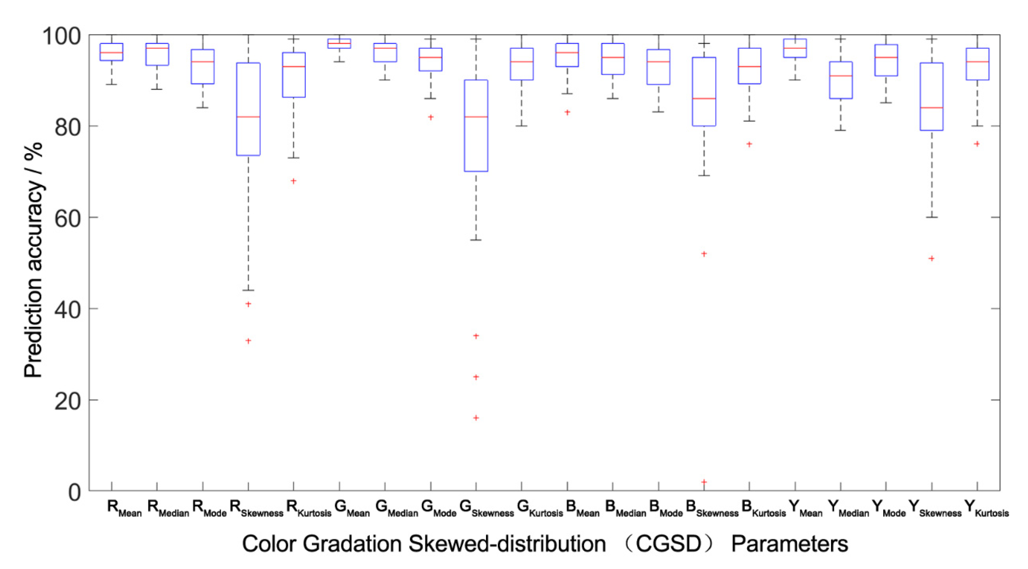
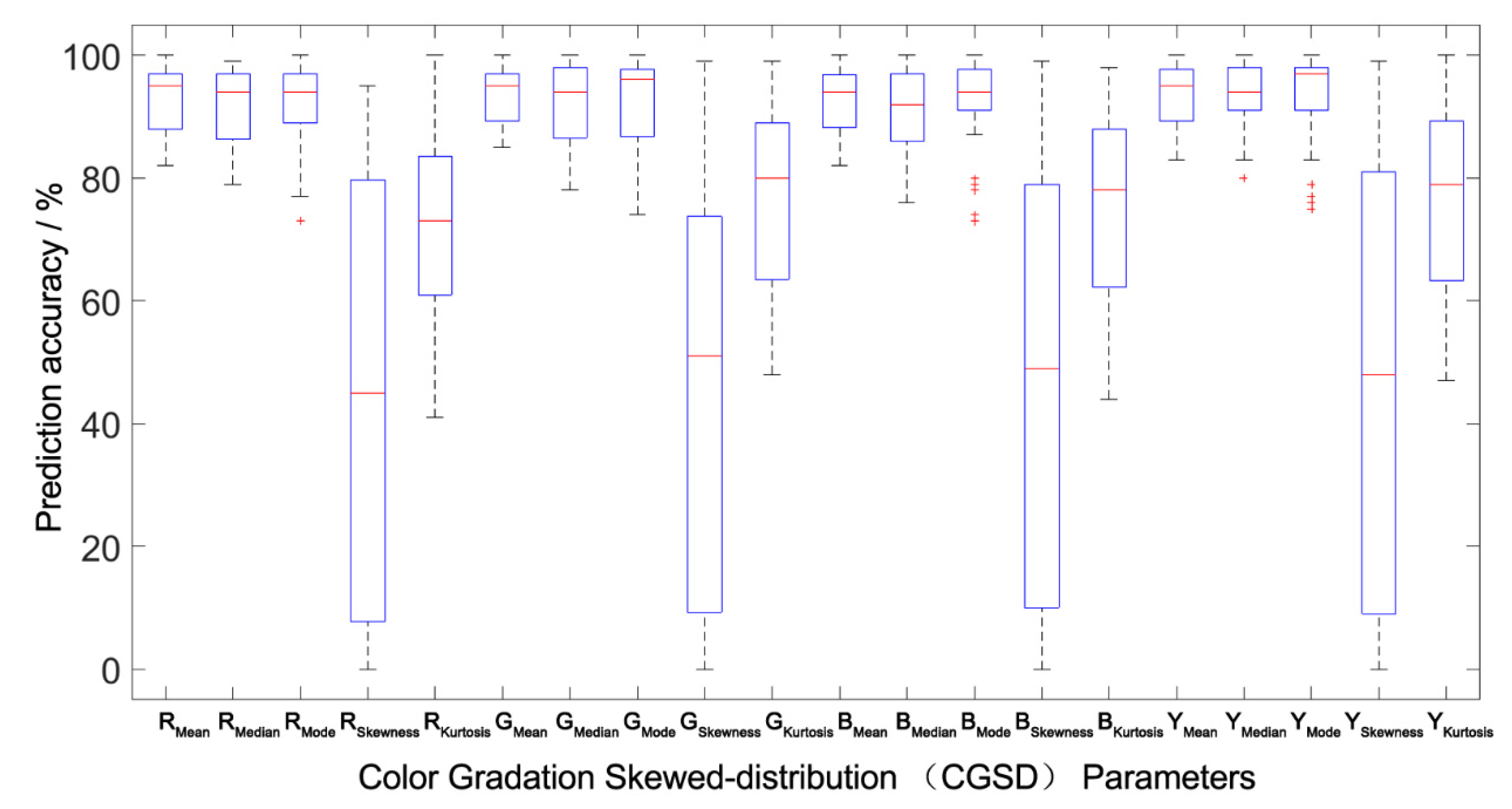
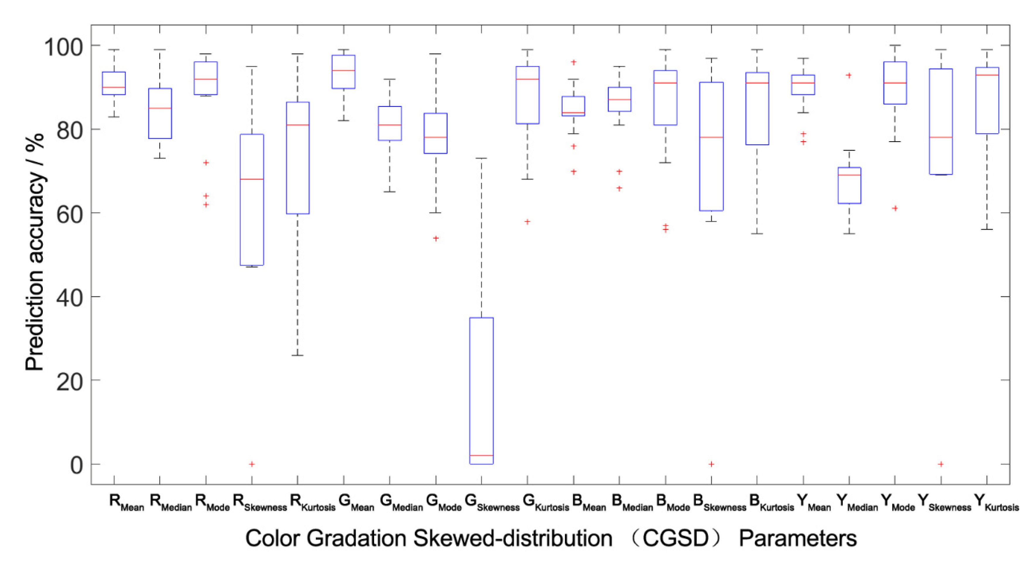
| RMean | Y1 | 51 | 0 | 96.27% | 51 | 0 | 92.89% | 15 | 0 | 90.92% | 94.11% |
| RMedian | Y2 | 51 | 0 | 96.02% | 51 | 0 | 91.98% | 15 | 0 | 84.90% | 92.84% |
| RMode | Y3 | 51 | 0 | 92.89% | 51 | 0 | 92.47% | 15 | 0 | 87.87% | 92.06% |
| RSkewness | Y4 | 51 | 0 | 80.98% | 51 | 10 | 53.21% | 15 | 3 | 70.30% | 68.80% |
| RKurtosis | Y5 | 51 | 0 | 90.48% | 51 | 0 | 72.53% | 15 | 0 | 73.56% | 80.49% |
| GMean | Y6 | 51 | 0 | 97.98% | 51 | 0 | 93.55% | 15 | 0 | 93.71% | 95.50% |
| GMedian | Y7 | 51 | 0 | 96.29% | 51 | 0 | 91.97% | 15 | 0 | 80.08% | 92.33% |
| GMode | Y8 | 51 | 0 | 94.14% | 51 | 0 | 92.38% | 15 | 0 | 77.33% | 91.22% |
| GSkewness | Y9 | 51 | 1 | 76.29% | 51 | 9 | 52.40% | 15 | 7 | 35.12% | 63.73% |
| GKurtosis | Y10 | 51 | 0 | 92.98% | 51 | 0 | 76.64% | 15 | 0 | 86.75% | 85.06% |
| BMean | Y11 | 51 | 0 | 95.46% | 51 | 0 | 92.05% | 15 | 0 | 84.66% | 92.59% |
| BMedian | Y12 | 51 | 0 | 94.53% | 51 | 0 | 90.57% | 15 | 0 | 85.42% | 91.64% |
| BMode | Y13 | 51 | 0 | 92.66% | 51 | 0 | 92.65% | 15 | 0 | 84.46% | 91.60% |
| BSkewness | Y14 | 51 | 1 | 82.21% | 51 | 8 | 56.11% | 15 | 3 | 82.39% | 72.36% |
| BKurtosis | Y15 | 51 | 0 | 92.17% | 51 | 0 | 74.21% | 15 | 0 | 84.12% | 83.31% |
| YMean | Y16 | 51 | 0 | 96.95% | 51 | 0 | 93.33% | 15 | 0 | 89.60% | 94.43% |
| YMedian | Y17 | 51 | 0 | 90.26% | 51 | 0 | 93.64% | 15 | 0 | 67.68% | 88.84% |
| YMode | Y18 | 51 | 0 | 94.11% | 51 | 0 | 93.15% | 15 | 0 | 87.27% | 92.82% |
| YSkewness | Y19 | 51 | 2 | 80.43% | 51 | 10 | 58.03% | 15 | 3 | 84.64% | 73.81% |
| YKurtosis | Y20 | 51 | 0 | 92.56% | 51 | 0 | 76.04% | 15 | 0 | 86.53% | 84.59% |
| Parameters | Model | R-Square | Adjusted R-Square | RMSE | Significant F | |
|---|---|---|---|---|---|---|
| RSkewness | Y4 | 0.803 | 0.791 | 0.142 | 0.000 | |
| Z1 | Equation (4) | 0.884 | 0.874 | 0.111 | 0.000 | |
| GSkewness | Y9 | 0.831 | 0.820 | 0.138 | 0.000 | |
| Z2 | Equation (5) | 0.902 | 0.893 | 0.107 | 0.000 | |
| BSkewness | Y14 | 0.791 | 0.782 | 0.145 | 0.000 | |
| Z3 | Equation (6) | 0.900 | 0.891 | 0.102 | 0.000 | |
| YSkewness | Y19 | 0.784 | 0.775 | 0.156 | 0.000 | |
| Z4 | Equation (7) | 0.894 | 0.884 | 0.111 | 0.000 | |
| Parameters | Model | Modeling Group | Between-Group | Outside-Group | Average | ||||||
|---|---|---|---|---|---|---|---|---|---|---|---|
| Prediction Sample Data | Eliminate Abnormal Data | Predictive Accuracy | Prediction Sample Data | Eliminate Abnormal Data | Predictive Accuracy | Prediction Sample Data | Eliminate Abnormal Data | Predictive Accuracy | |||
| RSkewness | Y4 | 51 | 0 | 80.98% | 51 | 10 | 53.21% | 15 | 3 | 70.30% | 68.80% |
| Z1 | 51 | 0 | 90.02% | 51 | 1 | 60.56% | 15 | 3 | 75.58% | 77.76% | |
| GSkewness | Y9 | 51 | 1 | 76.29% | 51 | 9 | 52.40% | 15 | 7 | 35.12% | 63.73% |
| Z2 | 51 | 0 | 88.31% | 51 | 1 | 60.82% | 15 | 3 | 73.71% | 74.60% | |
| BSkewness | Y14 | 51 | 1 | 82.21% | 51 | 8 | 56.11% | 15 | 3 | 82.39% | 72.36% |
| Z3 | 51 | 0 | 90.16% | 51 | 1 | 61.27% | 15 | 3 | 75.61% | 75.83% | |
| YSkewness | Y19 | 51 | 2 | 80.43% | 51 | 10 | 58.03% | 15 | 3 | 84.64% | 73.81% |
| Z4 | 51 | 0 | 89.05% | 51 | 1 | 60.10% | 15 | 3 | 82.34% | 75.53% | |
Publisher’s Note: MDPI stays neutral with regard to jurisdictional claims in published maps and institutional affiliations. |
© 2022 by the authors. Licensee MDPI, Basel, Switzerland. This article is an open access article distributed under the terms and conditions of the Creative Commons Attribution (CC BY) license (https://creativecommons.org/licenses/by/4.0/).
Share and Cite
Zhang, P.; Chen, Z.; Wang, F.; Wang, R.; Bao, T.; Xie, X.; An, Z.; Jian, X.; Liu, C. Response of Population Canopy Color Gradation Skewed Distribution Parameters of the RGB Model to Micrometeorology Environment in Begonia Fimbristipula Hance. Atmosphere 2022, 13, 890. https://0-doi-org.brum.beds.ac.uk/10.3390/atmos13060890
Zhang P, Chen Z, Wang F, Wang R, Bao T, Xie X, An Z, Jian X, Liu C. Response of Population Canopy Color Gradation Skewed Distribution Parameters of the RGB Model to Micrometeorology Environment in Begonia Fimbristipula Hance. Atmosphere. 2022; 13(6):890. https://0-doi-org.brum.beds.ac.uk/10.3390/atmos13060890
Chicago/Turabian StyleZhang, Pei, Zhengmeng Chen, Fuzheng Wang, Rong Wang, Tingting Bao, Xiaoping Xie, Ziyue An, Xinxin Jian, and Chunwei Liu. 2022. "Response of Population Canopy Color Gradation Skewed Distribution Parameters of the RGB Model to Micrometeorology Environment in Begonia Fimbristipula Hance" Atmosphere 13, no. 6: 890. https://0-doi-org.brum.beds.ac.uk/10.3390/atmos13060890