
Probability Forecasting of Short-Term Short-Duration Heavy Rainfall Combining Ingredients-Based Methodology and Fuzzy Logic Approach


Abstract
:1. Introduction
2. Data and Methods
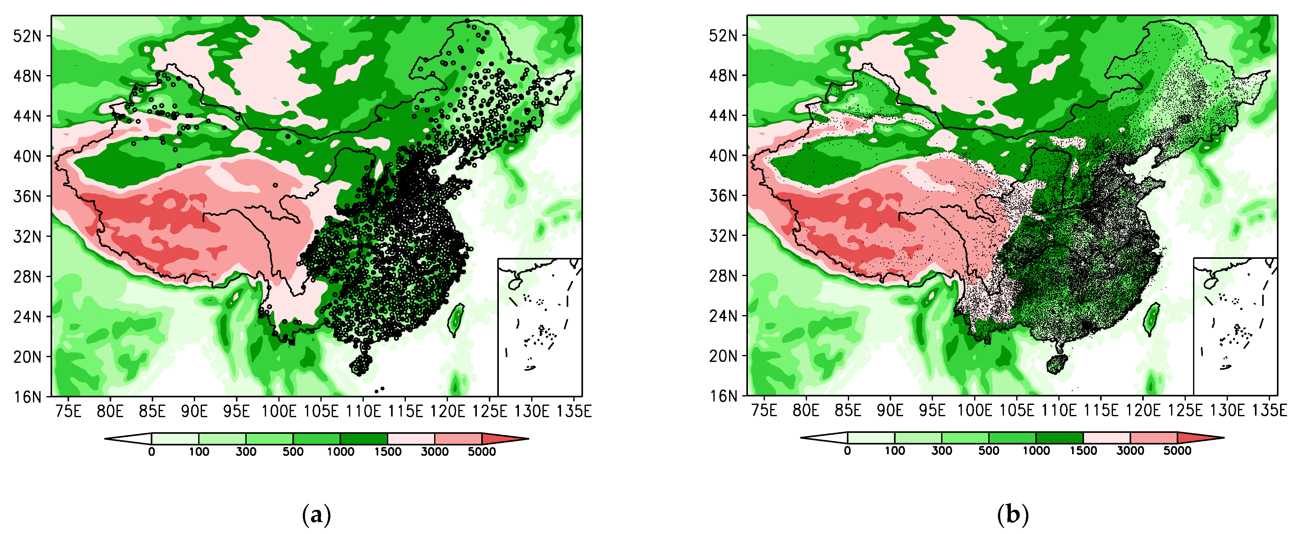
2.1. Data Source
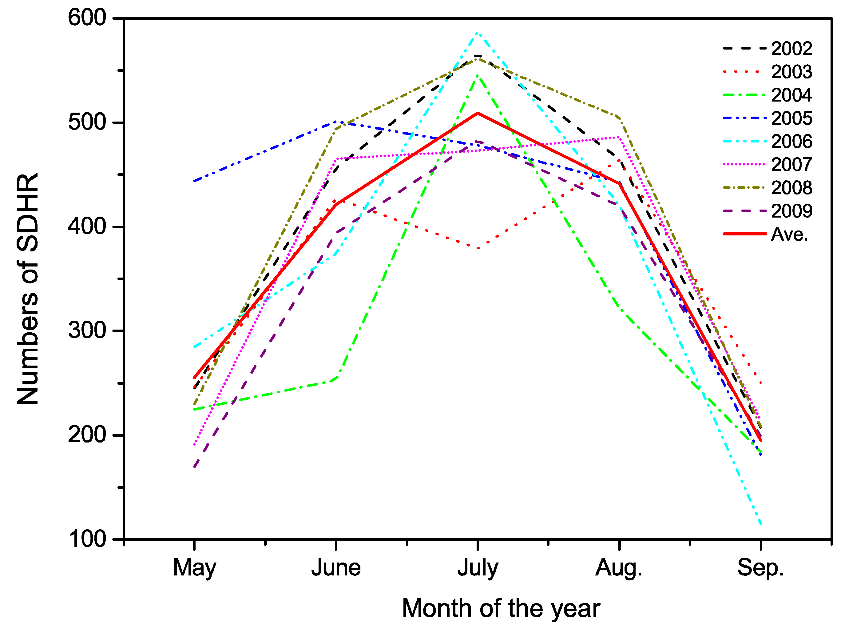
2.2. Climatology of SDHR
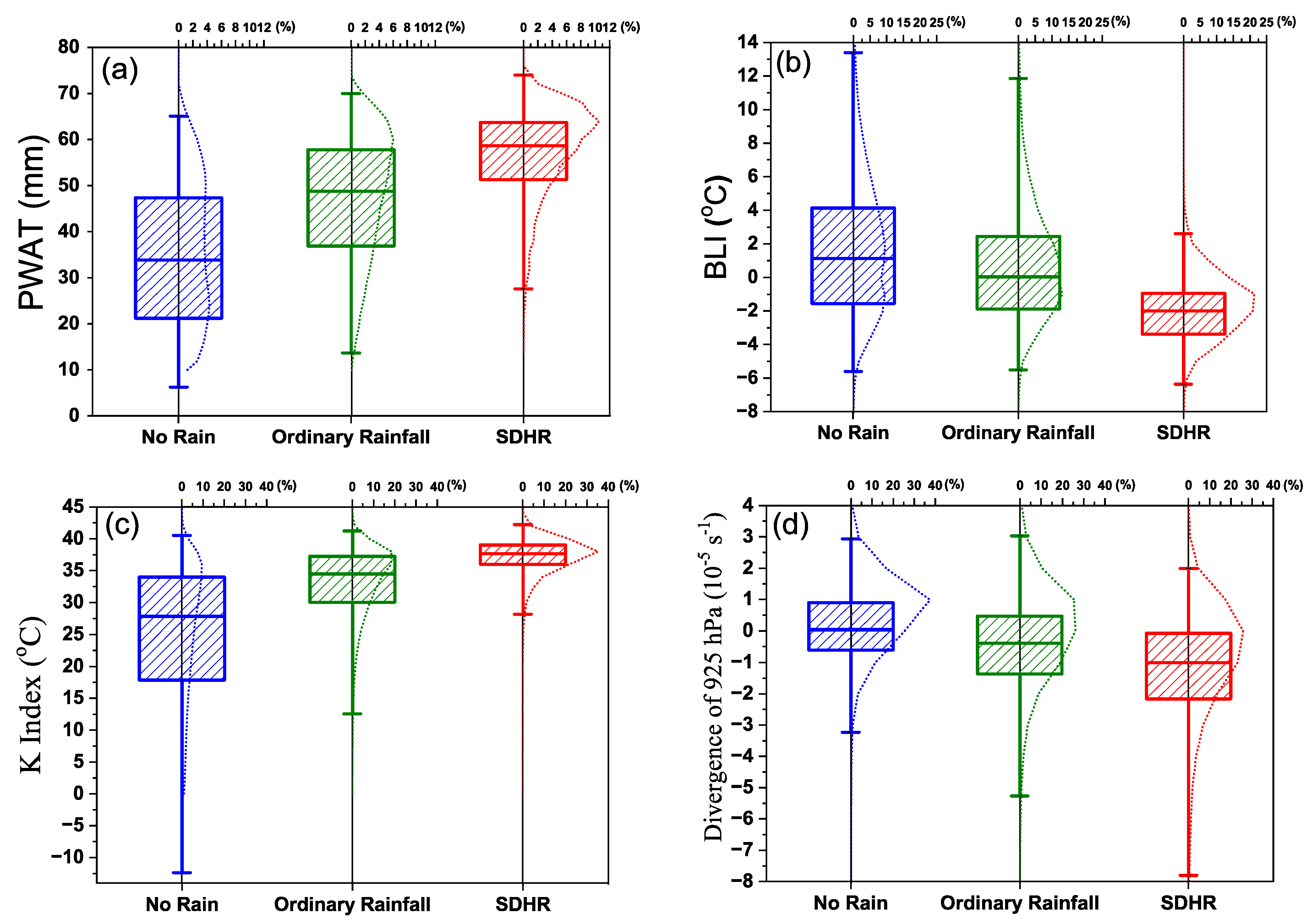
2.3. Selection of Predictors
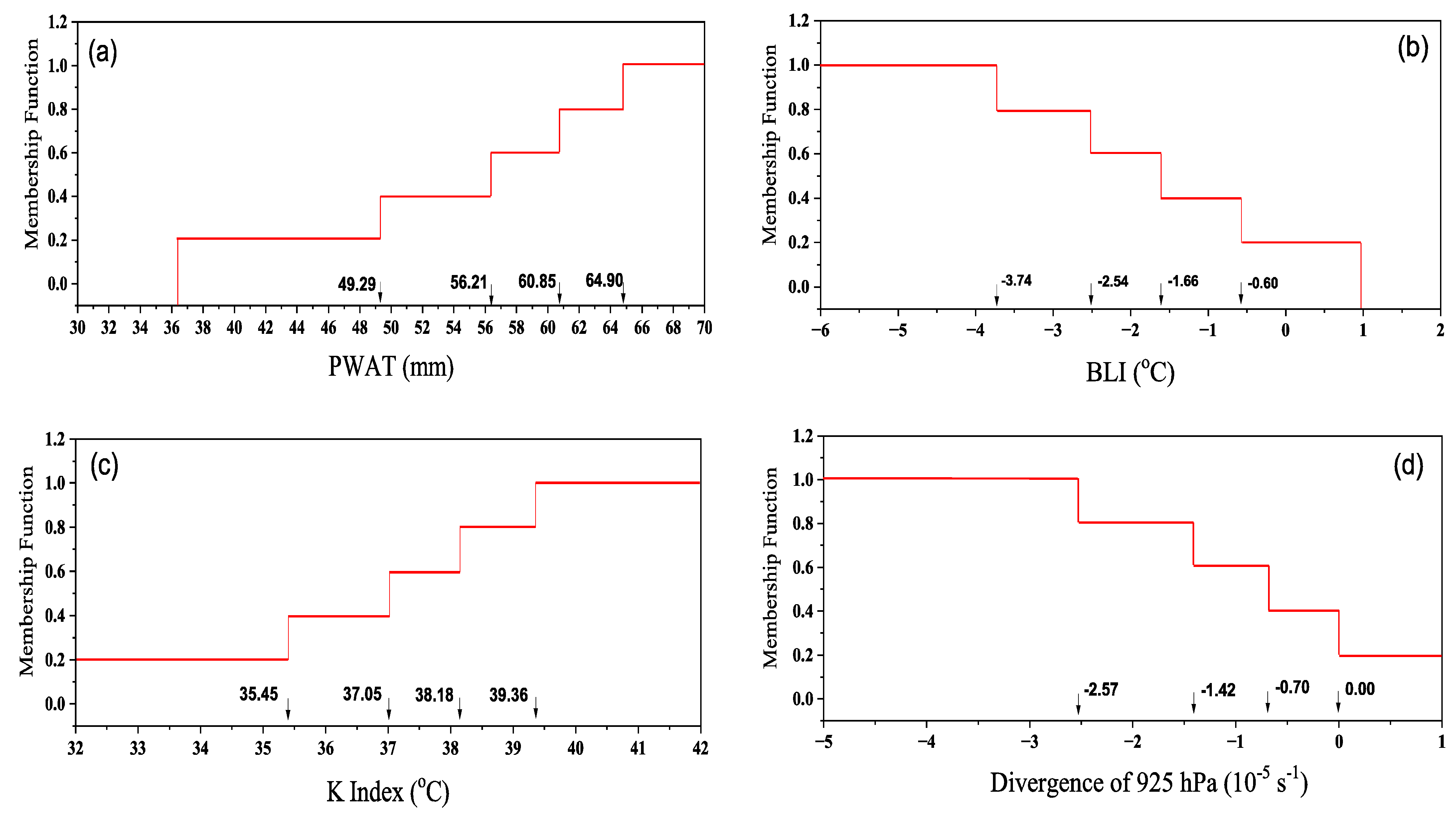
2.4. Fuzzy Logic Algorithm for the Probability of SDHR
2.5. Evaluation Method
3. Evaluation of Results
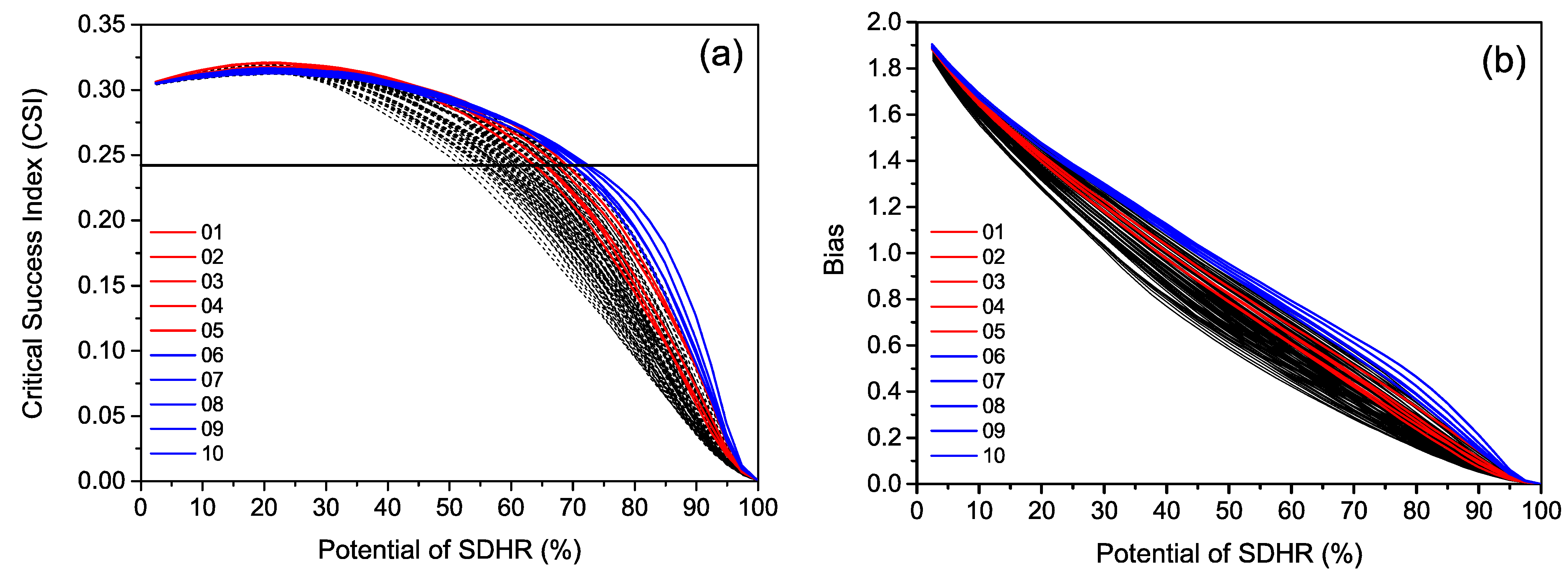
3.1. Evaluation for 00–12 h Forecasts
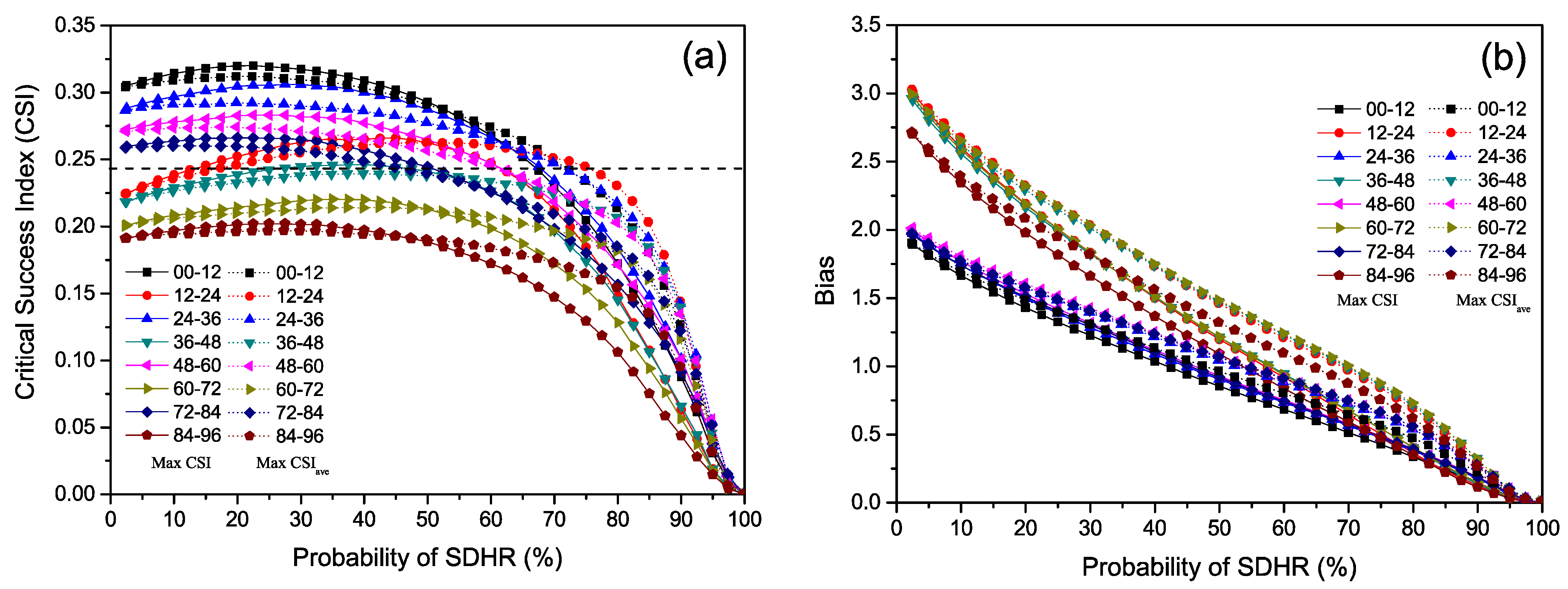
3.2. Evaluation of Longer Period Forecasts
4. Performance for Oceanic and Continental Events
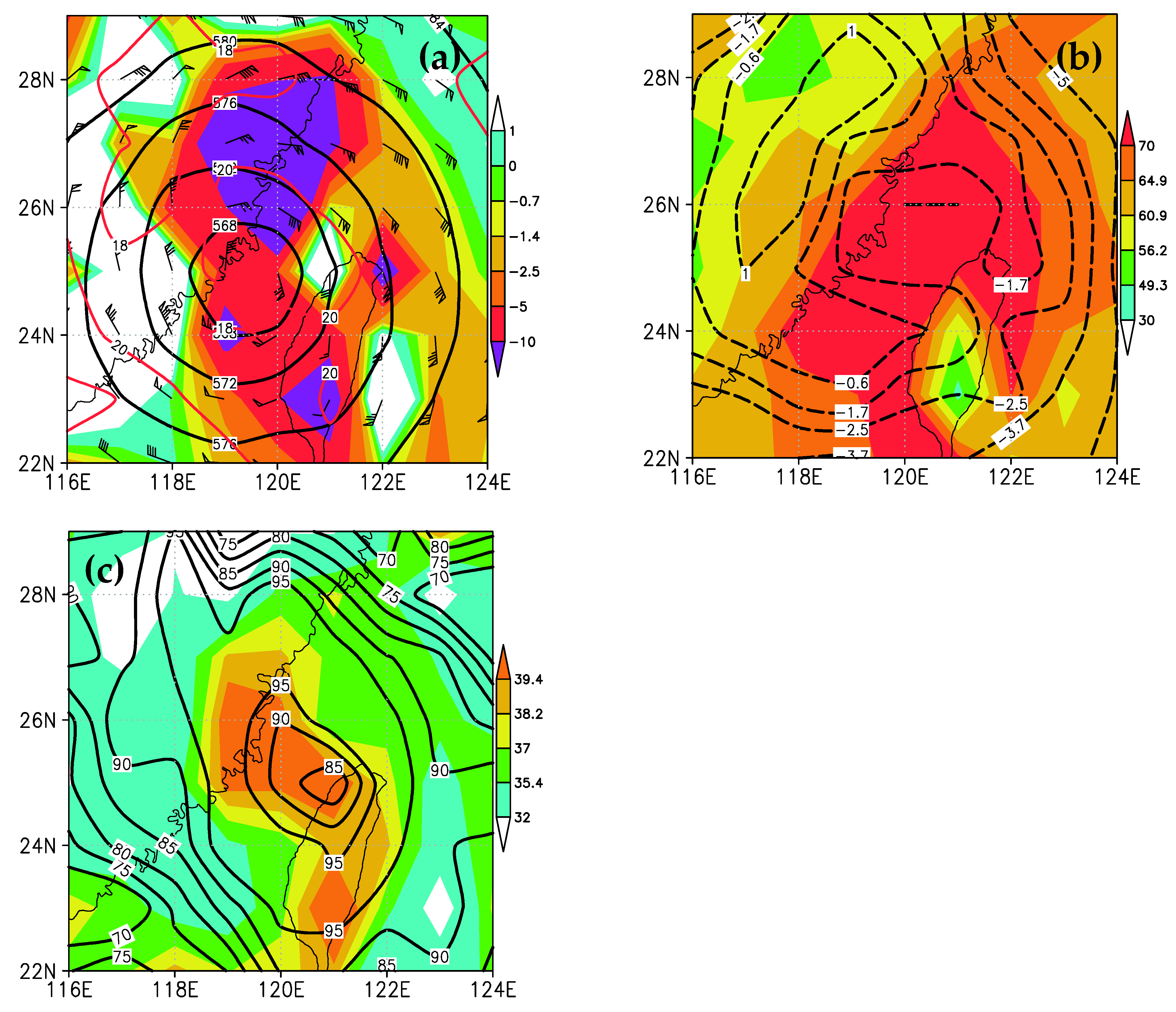
4.1. The Typhoon Soudelor on 8 August 2015
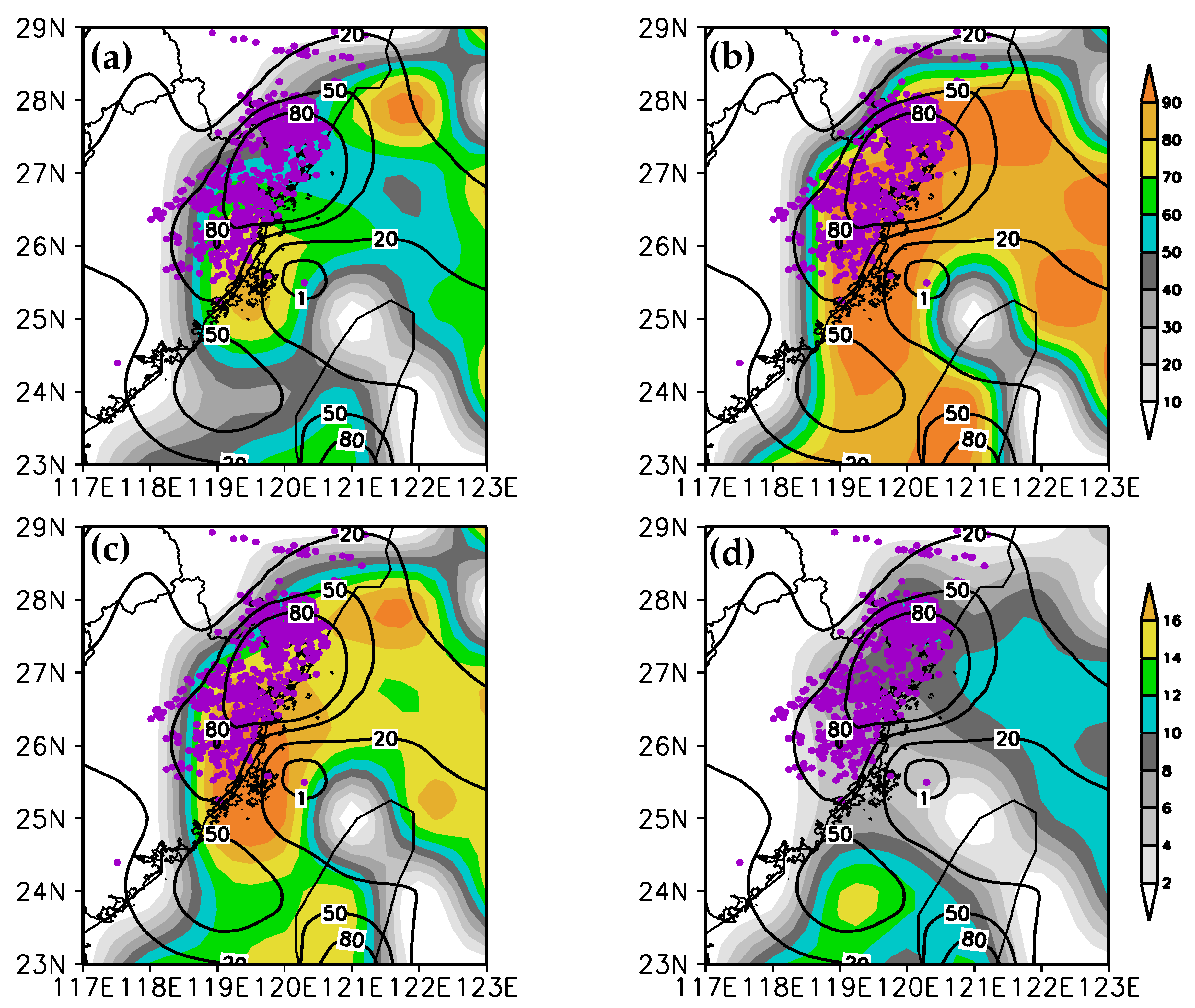
4.2. The Spring Event over Southern China on 15 May 2015
5. Conclusions and Discussion
Author Contributions
Funding
Institutional Review Board Statement
Informed Consent Statement
Data Availability Statement
Acknowledgments
Conflicts of Interest
References
- Brooks, H.E.; Stensrud, D.J. Climatology of heavy rain events in the United States from hourly precipitation observations. Mon. Weather Rev. 2000, 128, 1194–1201. [Google Scholar] [CrossRef] [Green Version]
- Hitchens, N.M.; Brooks, H.E.; Sshumachs, R.S. Spatial and temporal characteristics of heavy hourly rainfall in the United States. Mon. Weather Rev. 2013, 141, 4564–4575. [Google Scholar] [CrossRef]
- Luo, Y.L.; Wu, M.W.; Ren, F.M.; Li, J.; Wong, W.-K. Synoptic situations of extreme hourly precipitation over China. J. Clim. 2016, 29, 8703–8719. [Google Scholar] [CrossRef]
- Zheng, Y.G.; Gong, Y.D.; Chen, J.; Tian, F.Y. Warm-season diurnal variations of total, stratiform, convective, and extreme hourly precipitation over Central and Eastern China. Adv. Atmos. Sci. 2019, 36, 143–159. [Google Scholar] [CrossRef]
- Medlin, J.M.; Kimball, S.K.; Blackwell, K.G. Radar and rain gauge analysis of the extreme rainfall during Hurricane Danny’s (1997) landfall. Mon. Weather Rev. 2007, 135, 1869–1888. [Google Scholar] [CrossRef]
- Liao, Y.S.; Li, J.; Wang, X.F.; Cui, C.G.; Li, W.J. A meso-β scale analysis of the torrential rain event in Jinan in 18 July 2007. Acta Meteorol. Sin. 2010, 68, 944–956. (In Chinese) [Google Scholar]
- Yu, X.D. Investigation of Beijing extreme flooding on 21 July 2012. Meteorol. Mon. 2012, 38, 1313–1329. (In Chinese) [Google Scholar]
- Tian, F.Y.; Zheng, Y.G.; Zhang, X.L.; Zhang, T.; Lin, Y.J.; Zhang, X.W.; Zhu, W.J. Structure, triggering, and maintenance mechanism of convective systems during the Guangzhou extreme rainfall on 7 May 2017. Meteorol. Mon. 2018, 44, 469–484. (In Chinese) [Google Scholar]
- Yin, J.F.; Gu, H.D.; Liang, X.D.; Yu, M.; Sun, J.S.; Xie, Y.X.; Li, F.; Wu, C. A possible dynamic mechanism for rapid production of the extreme hourly rainfall in Zhengzhou City on 20 July 2021. J. Meteorol. Res. 2022, 36, 6–25. [Google Scholar] [CrossRef]
- Davis, R.S. Flash flood forecast and detection methods. In Severe Convective Storms; Doswell, C.A., III, Ed.; American Meteorological Society: Boston, MA, USA, 2001; pp. 481–525. [Google Scholar]
- Cao, Y.H.; Wu, Z.L.; Xu, Z.Y. Effects of rainfall on aircraft aerodynamics. Prog. Aerosp. Sci. 2014, 71, 85–127. [Google Scholar] [CrossRef]
- Yan, H.F.; Gallus, W.A., Jr. An evaluation of QPF from the WRF, NAM, and GFS Models using multiple verification methods over a small domain. Weather Forecast. 2016, 31, 1363–1379. [Google Scholar] [CrossRef]
- Huang, L.; Luo, Y.L. Evaluation of quantitative precipitation forecasts by TIGGE ensemble for south China during the presummer rainy season. J. Geophys. Res. Atmos. 2017, 122, 8494–8516. [Google Scholar] [CrossRef]
- Doswell, C.A., III; Brooks, H.E.; Maddox, R.A. Flash flood forecasting: An ingredients-based methodology. Weather Forecast. 1996, 11, 560–580. [Google Scholar] [CrossRef]
- Fankhauser, J.C. Estimates of thunderstorm precipitation efficiency from field measurements in CCOPE. Mon. Weather Rev. 1988, 116, 663–684. [Google Scholar] [CrossRef] [Green Version]
- May, P.T.; Rajopadhyaya, D.K. Vertical velocity characteristics of deep convection over Darwin, Australia. Mon. Weather Rev. 1999, 127, 1056–1071. [Google Scholar] [CrossRef]
- Lepore, C.; Allen, J.T.; Tippett, M.K. Relationships between hourly rainfall intensity and atmospheric variables over the Contiguous United States. J. Clim. 2016, 29, 3181–3197. [Google Scholar] [CrossRef]
- Lenderink, G.; Barbero, R.; Loriaux, J.M.; Fowler, H.J. Super-clausius-clapeyron scaling of extreme hourly convective precipitation and its relation to large-scale atmospheric conditions. J. Clim. 2017, 30, 6037–6052. [Google Scholar] [CrossRef]
- Nielsen, E.R.; Schumacher, R.S. Dynamical insights into extreme short-term precipitation associated with supercells and mesovortices. J. Atmos. Sci. 2018, 75, 2983–3009. [Google Scholar] [CrossRef]
- Doswell, C.A., III. The distinction between large-scale and mesoscale contribution to severe convection: A case study example. Weather Forecast. 1987, 2, 3–16. [Google Scholar] [CrossRef] [Green Version]
- Tang, W.Y.; Zhou, Q.L.; Liu, X.H.; Zhu, W.J.; Mao, X. Analysis on verification of national severe convective weather categorical forecasts. Meteorol. Mon. 2017, 43, 67–76. (In Chinese) [Google Scholar]
- Tian, F.Y.; Zheng, Y.G.; Zhang, T.; Mao, D.Y.; Tang, W.Y.; Zhou, Q.L.; Sun, J.H.; Zhao, S.X. Sensitivity analysis of short-duration heavy rainfall related diagnostic parameters with point-area verification. J. Appl. Meteorol. Sci. 2015, 26, 385–396. (In Chinese) [Google Scholar]
- Tian, F.Y.; Zheng, Y.G.; Zhang, T.; Zhang, X.L.; Mao, D.Y.; Sun, J.H.; Zhao, S.X. Statistical characteristics of environmental parameters for warm season short-duration heavy rainfall over Central and Eastern China. J. Meteorol. Res. 2015, 29, 370–384. [Google Scholar] [CrossRef]
- Li, Y.D.; Gao, S.T.; Liu, J.W. A calculation of convective energy and the method of severe weather forecasting. J. Appl. Meteorol. Sci. 2004, 15, 10–20. (In Chinese) [Google Scholar]
- Schmeit, M.J.; Kok, K.J.; Vogelezang, D.H.P. Probabilistic forecasting of (severe) thunderstorms in the Netherlands using model output statistics. Weather Forecast. 2005, 20, 134–148. [Google Scholar] [CrossRef]
- Pang, G.Q.; He, J.; Huang, Y.M.; Zhang, L.H. A binary logistic regression model for severe convective weather with numerical model data. Adv. Meteorol. 2019, 2019, 6127281. [Google Scholar] [CrossRef]
- Hill, A.J.; Herman, G.R.; Schumacher, R.S. Forecasting severe weather with random forests. Mon. Weather Rev. 2020, 148, 2135–2161. [Google Scholar] [CrossRef] [Green Version]
- Kistler, R.; Kalnay, E.; Collins, W.; Saha, S.; White, G.; Woollen, J.; Chelliah, M.; Ebisuzaki, W.; Kanamitsu, M.; Kousky, V.; et al. The NCEP-NCAR 50-Year Reanalysis: Monthly means CD-ROM and documentation. Bull. Am. Meteorol. Soc. 2001, 82, 247–268. [Google Scholar] [CrossRef]
- Chen, C.S.; Lin, Y.-L.; Zeng, H.-T.; Chen, C.-Y.; Liu, C.-L. Orographic effects on heavy rainfall events over northeastern Taiwan during the northeasterly monsoon season. Atmos. Res. 2013, 122, 310–335. [Google Scholar] [CrossRef] [Green Version]
- Tao, S.Y. Torrential Rain of China; Science Press: Beijing, China, 1980; pp. 1–225. (In Chinese) [Google Scholar]
- Trenberth, K.E. Atmospheric moisture recycling: Role of advection and local evaporation. J. Clim. 1999, 12, 1368–1381. [Google Scholar] [CrossRef]
- Galway, J.G. The lifted index as a predictor of latent instability. Bull. Am. Meteorol. Soc. 1956, 37, 528–529. [Google Scholar] [CrossRef] [Green Version]
- Zimmermann, H.J. Fuzzy Set Theory and Its Applications, 4th ed.; Springer Science & Business Media, LLC: Berlin, Germany, 2001; pp. 141–160. [Google Scholar]
- Mueller, C.; Saxen, T.; Roberts, R.; Wilson, J.; Betancourt, T.; Dettling, S.; Oien, N.; Yee, J. NCAR Auto-nowcast system. Weather Forecast. 2003, 18, 545–561. [Google Scholar] [CrossRef]
- Berenguer, M.; Sempere-Torres, D.; Corral, C.; Sanchez-Diezma, R. A fuzzy logic technique for identifying nonprecipitation echoes in radar scans. J. Atmos. Ocean. Technol. 2006, 23, 1157–1180. [Google Scholar] [CrossRef] [Green Version]
- Kuk, B.J.; Kim, H.I.; Ha, J.S.; Lee, H.K. A fuzzy logic method for lightning prediction using thermodynamic and kinematic parameters from radio sounding observations in South Korea. Weather Forecast. 2012, 27, 205–217. [Google Scholar] [CrossRef]
- Lin, P.-F.; Chang, P.-L.; Jou, B.J.-D.; Wilson, J.W.; Roberts, R.D. Objective prediction of warm season afternoon thunderstorms in northern Taiwan using a fuzzy logic approach. Weather Forecast. 2012, 26, 44–60. [Google Scholar] [CrossRef] [Green Version]
- Schroeer, K.; Kirchengast, G.; Sungmin, O. Strong dependence of extreme convective precipitation on gauge network density. Geophys. Res. Lett. 2018, 45, 8253–8263. [Google Scholar] [CrossRef] [Green Version]
- Chen, J.; Zheng, Y.G.; Zhang, X.L.; Zhu, P.J. Distribution and diurnal variation of warm-season short-duration heavy rainfall in relation to the MCSs in China. J. Meteorol. Res. 2013, 27, 868–888. [Google Scholar] [CrossRef]
- Li, W.H.; Yu, R.C.; Zhang, M.H.; Lin, W.Y.; Chen, H.M.; Li, J. Regimes of diurnal variation of summer rainfall over subtropical east Asia. J. Clim. 2012, 25, 3307–3320. [Google Scholar]
- Dai, Z.J.; Yu, R.C.; Li, J.; Chen, H.M. The characteristics of summer precipitation diurnal variation in three reanalysis datasets over China. Meteorol. Mon. 2011, 37, 21–30. (In Chinese) [Google Scholar]
- Zhou, C.L.; Wang, K.C. Contrasting daytime and nighttime precipitation variability between observations and eight reanalysis products from 1979 to 2014 in China. J. Clim. 2017, 30, 6443–6464. [Google Scholar] [CrossRef]
- Ren, F.M.; Yang, H. An overview of advances in typhoon rainfall and its forecasting researches in China during the past 70 years and future prospects. Torrent. Rain Disast. 2019, 38, 526–540. (In Chinese) [Google Scholar]
- Xu, W.X.; Zipser, E.J. Properties of deep convection in tropical continental, monsoon, and oceanic rainfall regimes. Geophys. Res. Lett. 2012, 39. [Google Scholar] [CrossRef]
- Schultz, D.M.; Cortinas, J.V.; Doswell, C.A., Jr. Comments on “An operational ingredients-based methodology for forecasting midlatitude winter season precipitation”. Weather Forecast. 2002, 17, 160–167. [Google Scholar] [CrossRef]
- Xu, W.X.; Zisper, E.J.; Chen, Y.-L.; Liu, C.; Liou, Y.-C.; Lee, W.-C.; Jou, B.J.-D. An orography-associated extreme rainfall event during TiMREX: Initiation, storm evolution, and maintenance. Mon. Weather Rev. 2012, 140, 2555–2574. [Google Scholar] [CrossRef] [Green Version]


| Classification | Abbr. | Indices | Unit | S1 | S2 | S |
|---|---|---|---|---|---|---|
| Moisture | PWAT * | Total precipitable water | mm | 0.70 | 0.41 | 0.287 |
| Q925 | Specific humidity of 925 hPa | g kg−1 | 0.70 | 0.49 | 0.343 | |
| RH850 | Relative humidity of 850 hPa | % | 0.75 | 0.42 | 0.315 | |
| Q850 | Specific humidity of 850 hPa | g kg−1 | 0.76 | 0.44 | 0.334 | |
| RH700 | Relative humidity of 700 hPa | % | 0.77 | 0.41 | 0.316 | |
| Q700 | Specific humidity of 700 hPa | g kg−1 | 0.78 | 0.40 | 0.312 | |
| DVF700 | Water vapor flux divergence of 925 hPa | g s−1 cm−2 hPa−1 | 0.80 | 0.65 | 0.520 | |
| DVF850 | Water vapor flux divergence of 850 hPa | g s−1 cm−2 hPa−1 | 0.90 | 0.78 | 0.702 | |
| DVF925 | Water vapor flux divergence of 700 hPa | g s−1 cm−2 hPa−1 | 0.98 | 0.97 | 0.951 | |
| Instability | BLI * | Best lifted index | °C | 0.52 | 0.47 | 0.244 |
| 925 hPa potential pseudo-equivalent temperature | K | 0.63 | 0.51 | 0.321 | ||
| 850 hPa potential pseudo-equivalent temperature | K | 0.64 | 0.45 | 0.288 | ||
| BCAPE | Best convective available potential energy | J kg-1 | 0.67 | 0.73 | 0.489 | |
| T850 | 850 hPa Temperature | °C | 0.68 | 0.66 | 0.449 | |
| KI* | K index | °C | 0.70 | 0.37 | 0.259 | |
| DT85 | Temperature difference of 850 hPa and 500 hPa | °C | 0.92 | 0.90 | 0.828 | |
| TT | Total totals | °C | 0.96 | 0.83 | 0.797 | |
| Lifting | SHR6 | 0–6 km vertical wind shear | m s−1 | 0.81 | 0.92 | 0.745 |
| DIV925 * | 925 hPa divergence | s−1 | 0.83 | 0.64 | 0.531 | |
| SHR3 | 0–3 km vertical wind shear | m s−1 | 0.88 | 0.71 | 0.625 | |
| DIV850 | 850 hPa divergence | s−1 | 0.92 | 0.90 | 0.828 | |
| SHR1 | 0–1 km vertical wind shear | m s−1 | 0.97 | 0.98 | 0.951 |
| Abbrev. | PWAT | RH850 | BLI | KI | DIV925 | T850 | TP |
|---|---|---|---|---|---|---|---|
| Unit | mm | % | °C | °C | S−1 | °C | mm |
| Threshold | ≥30 | ≥70 | ≤0.96 | ≥32.0 | ≤1.0 × 10⁻⁵ | ≥15 | ≥1.0 |
| Observation | |||
|---|---|---|---|
| Yes | No | ||
| Forecast | Yes | H (hit) | FA (false alarm) |
| No | M (miss) | CR (correct rejection) | |
| No. | Weights | Skill Scores | |||||||
|---|---|---|---|---|---|---|---|---|---|
| PWAT | BLI | DIV925 | KI | CSI | CSIave | Bias | POD | FAR | |
| 1 | 0.1 | 0.7 | 0.1 | 0.1 | 0.3202 | 0.2426 | 1.376 | 0.576 | 0.1234 |
| 2 | 0.2 | 0.6 | 0.1 | 0.1 | 0.3201 | 0.2357 | 1.416 | 0.586 | 0.1281 |
| 3 | 0.1 | 0.6 | 0.1 | 0.2 | 0.3199 | 0.2377 | 1.413 | 0.585 | 0.1278 |
| 4 | 0.1 | 0.5 | 0.1 | 0.3 | 0.3197 | 0.2333 | 1.339 | 0.567 | 0.1190 |
| 5 | 0.2 | 0.5 | 0.1 | 0.2 | 0.3197 | 0.2310 | 1.398 | 0.581 | 0.1261 |
| 6 | 0.1 | 0.1 | 0.7 | 0.1 | 0.3120 | 0.2501 | 1.477 | 0.589 | 0.1370 |
| 7 | 0.1 | 0.2 | 0.6 | 0.1 | 0.3130 | 0.2482 | 1.476 | 0.590 | 0.1367 |
| 8 | 0.1 | 0.3 | 0.5 | 0.1 | 0.3144 | 0.2465 | 1.475 | 0.592 | 0.1363 |
| 9 | 0.1 | 0.4 | 0.4 | 0.1 | 0.3157 | 0.2450 | 1.471 | 0.593 | 0.1355 |
| 10 | 0.1 | 0.1 | 0.6 | 0.2 | 0.3126 | 0.2443 | 1.456 | 0.585 | 0.1344 |
| 11 | 0.25 | 0.25 | 0.25 | 0.25 | 0.3165 | 0.2273 | 1.457 | 0.591 | 0.1269 |
Publisher’s Note: MDPI stays neutral with regard to jurisdictional claims in published maps and institutional affiliations. |
© 2022 by the authors. Licensee MDPI, Basel, Switzerland. This article is an open access article distributed under the terms and conditions of the Creative Commons Attribution (CC BY) license (https://creativecommons.org/licenses/by/4.0/).
Share and Cite
Tian, F.; Zhang, X.; Xia, K.; Sun, J.; Zheng, Y. Probability Forecasting of Short-Term Short-Duration Heavy Rainfall Combining Ingredients-Based Methodology and Fuzzy Logic Approach. Atmosphere 2022, 13, 1074. https://0-doi-org.brum.beds.ac.uk/10.3390/atmos13071074
Tian F, Zhang X, Xia K, Sun J, Zheng Y. Probability Forecasting of Short-Term Short-Duration Heavy Rainfall Combining Ingredients-Based Methodology and Fuzzy Logic Approach. Atmosphere. 2022; 13(7):1074. https://0-doi-org.brum.beds.ac.uk/10.3390/atmos13071074
Chicago/Turabian StyleTian, Fuyou, Xiaoling Zhang, Kun Xia, Jianhua Sun, and Yongguang Zheng. 2022. "Probability Forecasting of Short-Term Short-Duration Heavy Rainfall Combining Ingredients-Based Methodology and Fuzzy Logic Approach" Atmosphere 13, no. 7: 1074. https://0-doi-org.brum.beds.ac.uk/10.3390/atmos13071074