
Urban Heat Island and Thermal Comfort Assessment in a Medium-Sized Mediterranean City

Department of Environmental Engineering, Democritus University of Thrace, 67100 Xanthi, Greece
*
Authors to whom correspondence should be addressed.
Atmosphere 2022, 13(7), 1102; https://0-doi-org.brum.beds.ac.uk/10.3390/atmos13071102
Submission received: 14 June 2022
/
Revised: 5 July 2022
/
Accepted: 8 July 2022
/
Published: 13 July 2022
(This article belongs to the Special Issue Strategies for Mitigation and Adaptation to Urban Heat)
Abstract
:One of the greatest issues nowadays is that of the urban heat island effect on the thermal conditions inside cities. The air temperature inside the city core is warmer than that in suburbs, thus deteriorating the quality of life for citizens and making outdoor spaces uncomfortable in terms of thermal comfort. This phenomenon is usually assessed in large scale cities worldwide and less often in medium-sized towns. The current study aimed to investigate the urban heat island effect and, therefore, to assess the outdoor thermal comfort conditions in a medium-sized city. More specifically, the methodology of the current study includes: (i) the combination of different monitoring techniques to quantify the urban heat island effect in a medium-sized Mediterranean city. Both in situ measurements and remote sensing techniques were applied to assess the urban heat island effect in terms of both the canopy layer (CUHI) and the surface (SUHI); (ii) the identification of the parameters that affect thermal comfort and the identification of the most appropriate bioclimatic indices that determine outdoor thermal comfort in the city of interest. Both questionnaire survey and in situ measurements took place on a sidewalk in the city of Xanthi, Northern Greece, during the summer. The CUHI effect was obvious, especially in the morning and afternoon. Downscaled MODIS satellite images also showed that the intensity of SUHI was higher in the morning and afternoon. Apart from air temperature, important differences in the values of most microclimatic parameters were recorded between the meteorological station placed inside the urban area and those gathered from a nearby meteorological station. The narrow roads, the thermal properties of construction materials, and the absence of greenery characterized the area of interest and may be the key factors creating these differences in climate. Concerning the thermal comfort assessment, the most significant parameters were the air temperature and solar radiation, although, both empirical and direct indices were found to describe the comfort values well. According to the results, downscaling techniques are also important for the SUHI effect to be investigating in detail in medium-sized urban environments.
1. Introduction
Nowadays, globally, many people move from rural areas to the urban ones, thereby causing some issues in terms of climate. One of these issues is the urban heat island effect [1]. The urban heat island effect affects the quality of life of citizens and is responsible for thermal comfort conditions in both indoor and outdoor spaces [2]. Generally, there are four types of urban heat island effects [3]:
- ➢
- Surface urban heat island (SUHI)
- ➢
- Sub-surface
- ➢
- Canopy urban heat island (CUHI)
- ➢
- Boundary urban heat island (BUHI)
There are a lot of differences between these effects concerning the ways of assessing them and in the principles by which they are characterized. Generally, the BUHI is hard to assess because of the difference in temperature between sensor mounted on tall towers, air balloons and aircraft [4]. For this reason, the surface heat island effect (SUHI) and the canopy urban heat island effect (CUHI) are the most studied. Even though there are basic differences between them in terms of energetic and temporal characteristics, both are related to the result of changing agricultural areas to surfaces either without or with less vegetation [3]. There are several categories of observation of both CUHI and SUHI, such as in situ measurements, modelling approaches, remote sensing techniques, and infrared thermography. In situ measurement methods usually refer to the approach based on meteorological data gathered from mobile stations placed in different parts of the urban and rural areas [5,6]. The modelling approach usually refers to the method of using computer models. The ENVI-met model is an ordinary software tool used to assess microclimate and thermal comfort conditions [7,8]. Furthermore, a lot of computational fluid dynamics (CFD) simulation tools can calculate microclimate parameters [9]. The CUHI is usually assessed by comparing the air temperature inside an urban environment with that of a rural one [10,11]. Many studies conducted with in situ measurements and model simulations have shown that the UHI is characterized by seasonal variations [12,13]. Remote sensing techniques thermography are widely used for assessing the SUHI effect and offer detailed information on land surface temperature (LST) in various types of soil [14,15,16]. Various indices have been developed to characterize the impact of urbanization. One of these indices is the normalized difference vegetation index (NDVI) [17,18]. Finally, infrared thermography has also been widely applied because it can provide infrared images in greater detail at multiple scales. The UHI effect is usually observed at local or neighbourhood scales using aerial vehicles (AVs), rooftop observatories, drones, and portable cameras etc. [19,20].
The determination of human thermal comfort in outdoor spaces is of great importance when assessing the urban microclimate. Considering thermal comfort from the beginning will be quite helpful for building sustainable cities. According to ASHRAE, 2013 “Human comfort is defined as the condition of mind which expresses satisfaction with the thermal environment” [21]. A lot of effort has already been made worldwide on assessing the thermal sensation in outdoor environments [22].
For this reason, many models, called bioclimatic indices, have been developed to rate human thermal comfort in the outdoor environment. Bioclimatic indices are divided into the following categories [23]:
- ➢
- Rational indices
- ➢
- Empirical indices
- ➢
- Direct indices
Rational indices are mainly based on the energy balance of the human being taking into consideration the interactions between metabolic work rate, clothing insulation, and meteorological parameters, on the thermal perception of the pedestrian. One of the most well-known indices is the Predicted Mean Vote (PMV) [24,25]. Although the PMV index was used to evaluate thermal comfort in indoor environment at first [26], it was recently applied to assess thermal comfort outdoors [27,28]. Another rational index that is extensively used is the Physiological Equivalent Temperature (PET), “based on the Munich Energy-balance model for Individuals” [29]. A well-known rational index is the ‘Standard Effective Temperature (SET)’ based on the Pierce two-nodes model which simplifies the complex environment into a standard environment [30]. Finally, the ”Universal Thermal Climate Index (UTCI)“ is a relatively newly developed rational index, which is based on a multi-node heat budget based approach and is extensively used in many case studies [31,32].
On the other hand, ‘Empirical indices’ rate thermal comfort for a specific climatic location and are expressed as linear equations that are based on in situ measurements and questionnaire surveys. The ‘Wet-Bulb Globe Temperature (WBGT)’ is one of these indices and is one of the most extensively used biometeorological indices [33]. The ‘WBGT’ was initially used to evaluate thermal stress at training camps of the United States Army and, more recently, it was used to assessing thermal comfort of outdoor spaces [34]. The ‘Actual Sensation Vote (ASV)’ is also an empirical index developed by the RUROS project. The ‘ASV index’ is based on both in situ microclimatic measurements and questionnaire data in different countries across Europe [35].
Finally, the direct indices that are based on linear equations, assess thermal comfort by considering the impact of meteorological parameters such as air temperature, wind speed, and relative humidity. There are a lot of widely used direct indices. The ‘Normal Effective Temperature (NET)’ [36] as well as the ‘Apparent Temperature (AT)’ [37,38] and the Heat Index (HI) [36,39] are used to rate thermal comfort in a warm environment, while the ‘Wind Chill Index (WCI)’ [40] is used to measure thermal stress in a cool environment.
The phenomenon of the urban heat island effect and the assessment of outdoor thermal comfort conditions is usually examined in large scale urban areas and not so much in small or medium scale towns [41]. The aim and the original contribution of the current study was to: (i) Assess the phenomenon of the urban heat island effect in a medium-sized Mediterranean city through different monitoring techniques to identify both the CUHI and SUHI effects. Both techniques were used so that the urban heat island effect in the region could be quantified in detail. Apart from quantifying the UHI effect, surface temperature data that was extracted from satellite data was compared with air temperature, so the correlation between them could be assessed. Apart from surface temperature, the distribution of air temperature derived from satellite images would create a more holistic view allowing the hot spots in medium-sized cities to be effectively identified. (ii) Assess thermal comfort conditions of outdoor spaces, to derive the most appropriate bioclimatic indices and to extract city comfort indices to represent thermal comfort in medium-sized cities. In situ monitoring and a questionnaire survey were carried out in summer and several statistical techniques were used to elaborate the obtained data in order to assess the outdoor thermal comfort conditions in the city of Xanthi, Northern Greece.
2. Methodology
In the current study, the investigation of the heat island effect in a medium-sized city was based on data from both in situ monitoring measurements and satellite images and used for microclimatic analysis. A modelling approach was used when infrared thermography was not being considered. Concerning the modelling approach, limitations such as the complexity of the geometry and issues regarding the initialization of data, very often lead to simulation errors [42,43,44]. On the other hand, assessing the urban heat island effect at the city scale via infrared thermography can be costly as thermal cameras are normally installed on aircrafts or on helicopters [19]. The satellite data analysis included, the acquisition of several satellite images covering the study area, selection of the most appropriate ones (excluding cloudless conditions) and application of downscaling techniques to derive high resolution data for the microclimate of the study area. These data were compared with in situ measurements carried out during summer in the study area. Meteorological data from a nearby meteorological station were also acquired. For the thermal sensation analysis in the study area, an in situ monitoring campaign was combined with the distribution of questionnaires to users of the area during summer. For the thermal sensation analysis and the thermal comfort prediction, several statistical techniques were applied to the acquired data that were interpreted into bioclimatic indices. Different indices were investigated and the most appropriate ones for thermal comfort prediction in the study area were proposed.
2.1. Monitoring Procedure
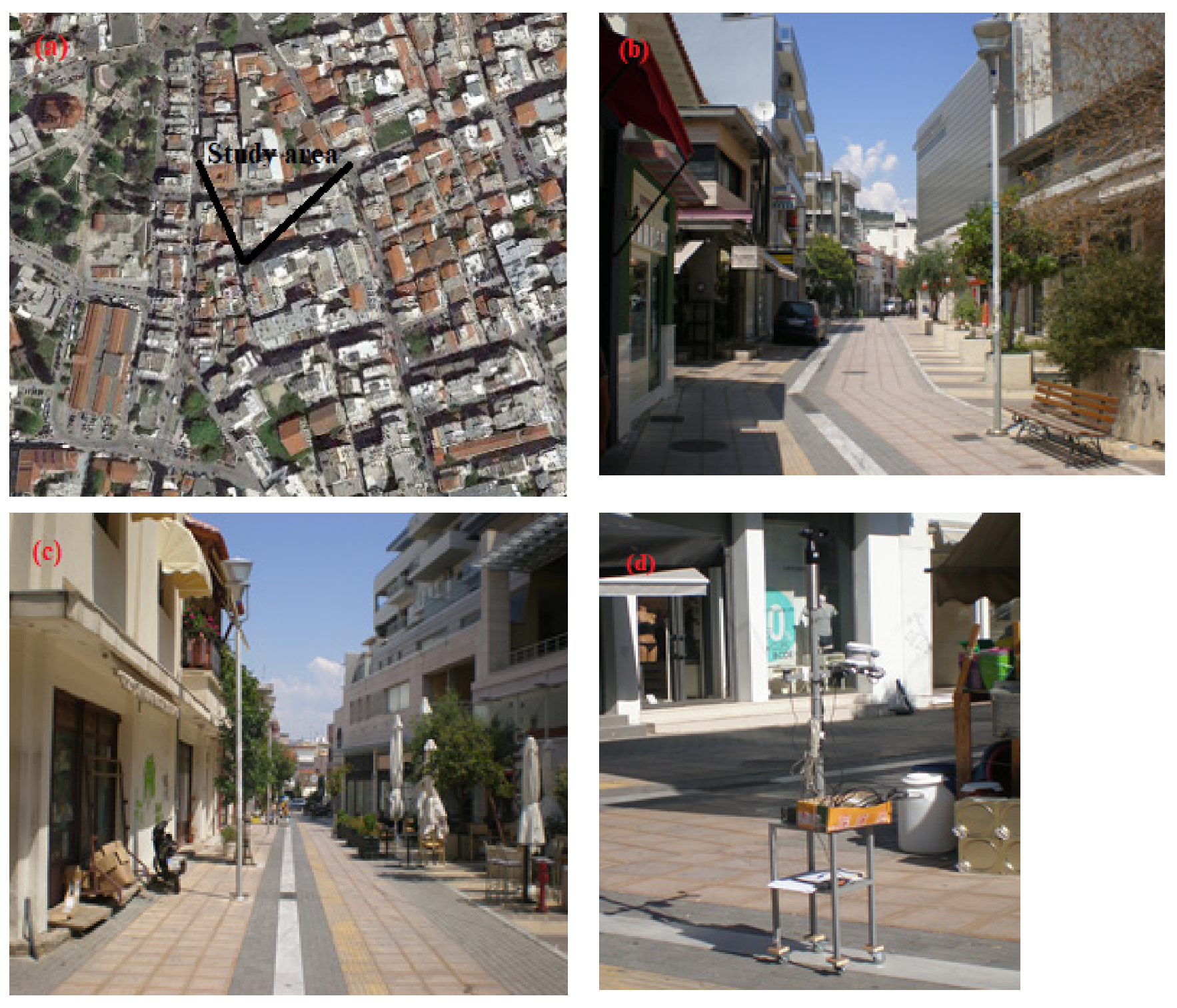
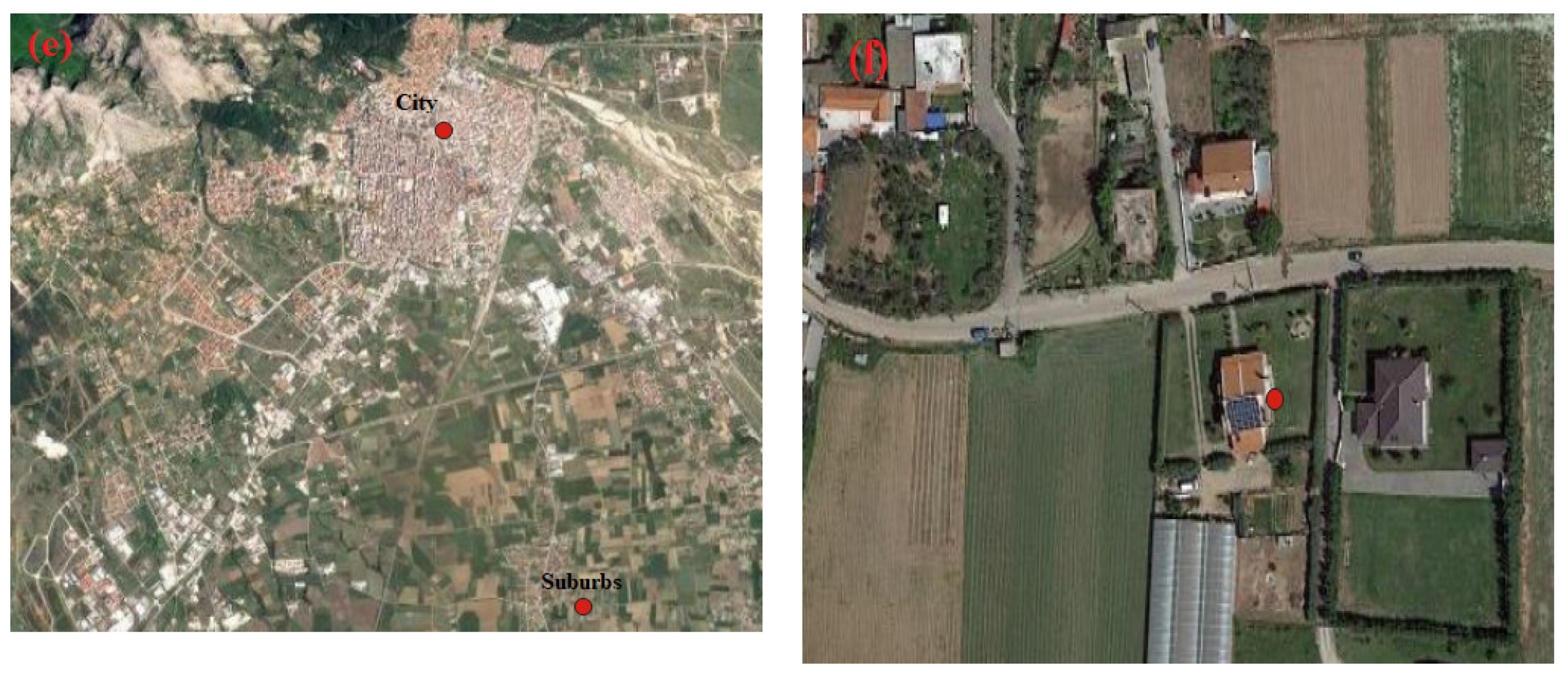
The study was located in a pedestrian area in the city of Xanthi, Northern Greece Figure 1a–c, located at 41°08′ N latitude, 24°53′ E longitude and 43 m altitude [45]. The selected site represented an ordinary urban morphology with commercial buildings, small entertainment places like coffee restaurants, block of flats, and a low amount of vegetation. Furthermore, a lot of people visit the study site, or work in the commercial buildings daily, so many questionnaires were dispensed. The microclimate conditions in the area were monitored with a mobile meteorological station, Figure 1d. Additionally, meteorological data from a weather station located in a rural area almost 4.5 km from the city of Xanthi—the weather station of the National Observatory of Athens located in the region of Peteinos (41°05′56″ N latitude 24°53′10″ E longitude and 40 m altitude)—were collected [46], Figure 1e,f. The study was conducted during the summer of the year 2016, between July 16 and August 6 (21 days). This period of the year was selected as the weather conditions are usually stable and, according to available historic weather data, the mean monthly air temperature appears to be at its peak [45].
2.2. In Situ Measurements
Microclimatic measurements were carried out near the interviewees with a mobile meteorological station (Figure 1d), for air temperature (Tair), relative humidity (RH), globe temperature (Tglobe), and solar radiation (SR) at 1.5 m above ground, and the wind speed (WS) at 2 m above ground. The heights chosen for taking measurements were selected because they represent the conditions that prevail at the pedestrian level.
The globe temperature was measured with a tailor-made thermometer for outdoor measurements, a thermistor sensor positioned in the middle of a hollow, grey acrylic sphere of 0.038 m diameter [47]. The grey colour was used as it represents the radiant properties of the human skin and the most common clothing insulation for an ordinary person. This globe thermometer had a response time of less than 5 min, in correspondence with measurements of Tair, and WS, and it has been proven to be a suitable instrument to assess the outdoor mean radiant temperature (Tmrt) [47]. The mean radiant temperature was calculated from Equation (1) [48]:
where ε is the emissivity (0.95) and D the diameter of the sphere material (0.038 m). The technical details of the measuring instruments that were used in the current study are shown in Table 1.
The measurements were carried out at three different periods of the day: morning (10:00 to 11:30 a.m.), afternoon (13:10 to 14:40) and evening (19:10 to 20:40).
Remote Sensing
Remote sensing techniques were applied to identify the ‘surface urban heat island’ effect (SUHI). More specifically, numerous satellite images were gathered through the monitoring period. The selected sensor was that of MODIS and the products MOD11A1, MOD11A2, MYD11A1, MYD11A2 were used [49]. Both MOD11A1 and MYD11A1 provide land surface temperature daily at a 1 km spatial resolution, while MOD11A2 and MYD11A2 were available every 8 days. All products provide day and night data. Even though all products offer low spatial resolution, they give the opportunity for the UHI to be assessed in greater detail. The acquisition of these data is free of charge, and they provide at least four data points on a daily basis, observing in that way the trend of the UHI during the day. The MOD11A2 and MYD11A2 where selected for this study to overcome possible cloud contaminated MOD11A1 and MYD11A1 products. Table 2 presents the product details [50].
Downscaling Methodology
Although the MODIS satellite offers low spatial resolution data, it however offers high revisit periodicity. On the other hand, several satellites with low temporal frequency, such as Landsat and Sentinel, provide high volumes of analysis data [51]. For this reason, a downscaling technique is of great importance for satellite data to be used more frequently. The most well-known technique is the statistical downscaling (thermal sharpening). Thermal sharpening uses the parametric relationship of the LST (land surface temperature) and ancillary data. A lot of regression models have already been developed, such as: Disaggregation of Radiometric Temperature (DisTrad), Temperature Sharpening (TsHARP), and the TsHARP with local variant. In the DisTrad downscaling model, the inverse relationship between temperature and indices that are uses to quantify vegetation covered areas was applied [52]. The TsHARP model is considered to be a modification of the DisTrad method that is more accurate. For this reason, the fractional vegetation cover (FVC) was used [53]. Accordingly, the TsHARP model with local variant is a modification of the TsHARP method, enhancing the accuracy in mixed agricultural cover areas [54]. Pixel, modulation techniques in urban areas were also applied using high resolution emissivity data [55]. Finally, a new statistical downscaling approach that used land surface emissivity was developed, and it showed accurate result compared to the Advanced Spaceborn Thermal Emission and Reflection Radiometer (ASTER) land surface temperature data in urban areas [56].
In the current study, the TsHARP technique was used. Both Sentinel-2 (S2) data (resolution 10–60 m) and Landsat 8 data (resolution 30 m) were selected for the downscaling procedure along with the MODIS satellite images. This method was selected as previous studies have shown satisfactory results concerning the disaggregation of MODIS to Landsat spatial resolution [57]. The Sentinel-2 image data, acquired on 30 July 2016, and that of Landsat 8, acquired on 6 August 2016, were used. The spectral information of the selected channels is presented in Table 3 [58,59,60,61]. In both satellite sensors, the visible red (RED) and near infrared (NIR) bands were both used so that the normalized difference vegetation index (NDVI) could be calculated.
The NDVI index was created to identify vegetation covered areas and its values vary from −1 to +1 and it is calculated as follows (Equation (2)) [62,63]:
where NIR is the near infrared band and Red, the red band of the selected sensor. High values of NDVI show vegetated areas, and low values show water and bare soil areas.
The selected downscaling technique was based on the reverse relationship of LST and NDVI and it is developed as follows [52,53,64,65]:
where, NDVICR is the NDVI in low resolution analysis and is the predicted LST at low resolution; LSTREF refers to reference LST and is the residual temperature of low resolution; NDVIHR refers to the NDVI index in high resolution analysis; and refers to predicted LST at high resolution analysis. For the TsHARP method, the slope and the intercept values were calculated as follows:
Both LST retrieval and downscaling procedure were processed in RStudio, an integrated development environment for programming language, R [66].
2.3. Outdoor Thermal Comfort Survey
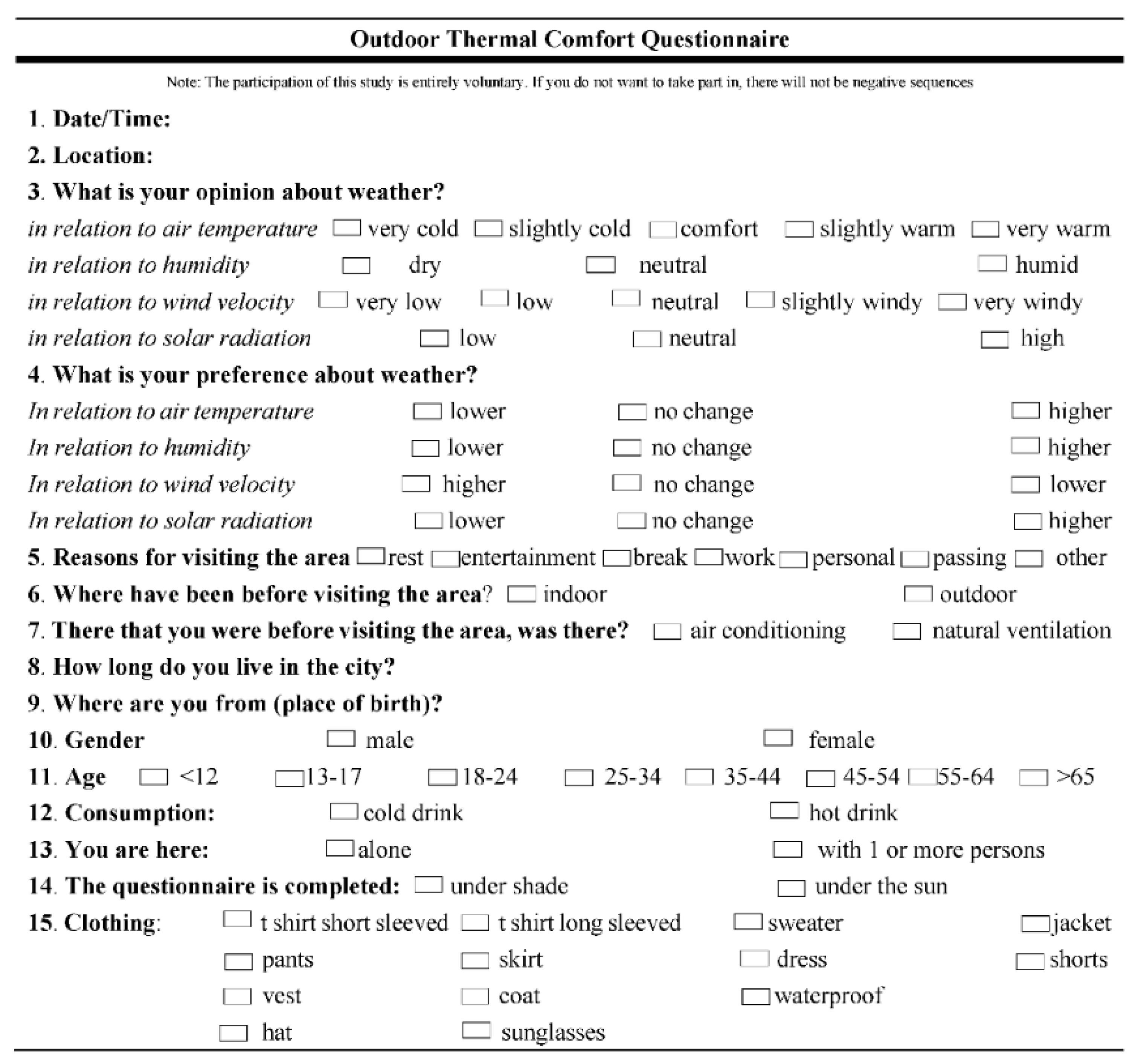
The questionnaires were distributed randomly to people who were visiting the study area while in situ measurements were made. The questionnaire was divided into three parts. The first part included questions expressing the opinion of the interviewee about the sensation of the climatic parameters (air temperature, humidity wind velocity, and solar radiation). All responses to these questions were analysed on a 5-point scale (air temperature, wind tolerance) or in a 3-point scale (solar radiation, humidity). Respondents were asked to rate their thermal comfort on a 5-point scale (Actual Sensation Vote (ASV)) (−2 stands for “very cold”; −1 for “slightly cold”; 0 for “comfort”; 1 for “slightly warm”; 2 for “very warm”) [35]. Both a 5-point scale and a 7-point scale of thermal sensation have been widely used [67,68]. The 7-point scale was used as the thermal sensation scale [69] and was proposed by ISO 10551 [70]. However, in the current study, the ASV index was chosen because it is a usual method for the assessment of outdoor thermal comfort and it has been already adopted in previous research that has taken place in Greece [71,72]. The second part of the questionnaire includes personal information (e.g., age, gender, clothing insulation etc.) and the third part includes psychological parameters (reason of visiting the area) and other social aspects. Clothing insulation values were derived from the clothing description of the respondents [73]. Totally, 266 questionnaires were selected, approximately 12 per day. In the Appendix A, the questionnaire that was used in the study is shown.
2.4. Thermal Sensation Analysis
Based on the questionnaire and weather monitoring data, the factors related to thermal sensation were assessed. The parameters that were examined were separated into three main categories: meteorological, personal, and physiological, and two statistical procedures were applied:
- (1)
- One-way ANOVA was used to define the relationship between ASV and each parameter to be defined.
- (2)
- The ordinal regression analysis was used for determination of the parameter that was related to thermal sensation.
2.5. Thermal Comfort Calculation
This research examined the applicability of 18 thermo-physiological indices for the climate of Xanthi. The selected indices were based on the Silvia Coccolo’s list, which they divided into three categories [74]: rational, empirical, and direct indices. In Table 4, the characteristics of the selected indices are presented. The ASVATHENS was chosen instead of the ASVTHESSALONIKI and the ASVMEDITERRANEAN as it has already shown to be the most applicable to Mediterranean climates [75]. Additionally, the MOCI was included in empirical indices, however, it is a new index that rates thermal comfort in Mediterranean climates [76]. Finally, the Wind Chill Index (WCI) was not examined as it is usually applied in cold environments [40].
The rational indices PMV, PET, OUT_SET, UTCI and PT were calculated using the RayMan model for each, one interview separately, and they were compared with the actual sensation vote (ASV). The RayMan model was developed according to Guideline 3787 of the German Engineering Society and can calculate the radiation flux in both simple and complex environments [77,78]. The body surface area for men was standardized to 1.98 m2, which represents a human with height equal to 1.77 m and a body weight equal to 80 kg. Accordingly, body surface for women was set at 1.67 m2 (1.66 height and 60 kg weight). These data were acquired from the investigation done by Pantavou et al. (2013) from 1706 questionnaires in the Mediterranean city of Athens and assumes that there are negligible differences in the population among Greek cities [79]. Metabolic activity was set at 58.2 W/m2, which is equivalent to energy produced by a person who is seated at rest [80,81], as all respondents filling the questionnaire were resting. ‘Empirical’ and ‘Direct’ indices were calculated according to Table 5.

Table 4.
Characteristics of the selected indices.
| Category | Abbreviation | Index | Reference |
|---|---|---|---|
| Rational indices | PMV | Predicted Mean Vote | [24,25] |
| PET | Physiologically Equivalent Temperature (°C) | [29] | |
| OUT_SET | Outdoor Standard Effective Temperature (°C) | [30] | |
| UTCI | Universal Thermal Climate Index (°C) | [31] | |
| PT | Perceived Temperature (°C) | [82] | |
| Empirical indices | ASVATHENS | Actual Sensation Vote | [35,83] |
| TS | Thermal Sensation | [84,85] | |
| TSP | Thermal Sensation Perception | [86] | |
| MOCI | Mediterranean Outdoor Comfort Index | [76] | |
| WBGT | Wet Bulb Globe Temperature (°C) | [87,88] | |
| Direct indices | AT | Apparent Temperature (°C) | [37,38] |
| DI | Discomfort Index (°C) | [89] | |
| ESI | Environmental Stress Index (°C) | [90,91] | |
| NET | Normal Effective Temperature (°C) | [36] | |
| HU | Humidex (°C) | [92] | |
| HI | Heat Index (°C) | [36,39] | |
| CP | Cooling Power Index (mcalm−2/s) | [93] | |
| RSI | Relative Strain Index (°C) | [94] |
To evaluate the human thermal sensation, the relationship between the mean Actual Sensation Vote (mASV) value and those of every one of the calculated indices were separately examined. In the case of PET, OUT_SET, UTCI, PT, AT, DI, ESImodified, NET, HU, HI and WBGT, the ‘Mean Actual Sensation Vote’ (mASV) of the respondents in each 1 °C of these indices’ interval groups was separately calculated. Accordingly, in the case of PMV, TS, TSP, MOCI and CP, the mean Actual Sensation Vote (mASV) of the respondents in each 1 unit of PMV, TS and CP interval group was calculated separately. Finally, in the case of ASVATHENS and RSI, the mean Actual Sensation Vote (mASV) was calculated in each 0.1 unit of these indices.
3. Results
3.1. Weather Data
During the survey period, air temperature ranged from 26.9 to 43.7 °C, relative humidity from 15 to 56%, wind speed from 0.5 to 4.6 m/s, mean radiant temperature from 26.2 to 50.3 °C, and solar radiation from 1 to 1290 W/m2 (Table 6). The air temperature measured by the thermistor in a white shielded box was quite close to that measured by the HOBO Pro V2 sensor; the mean difference of the values was 0.4 °C. The sky was generally clear and sunny. The minimum mean air temperature was recorded on 20 July 2016 (31 °C) (day 4) and the maximum on 6 August 2016 (37.1 °C) (day 21). Considering all recorded days, the average values were: air temperature 35.4 °C, relation humidity 56%, wind speed 4.6 m/s, mean radiant temperature 47.1 °C, and solar radiation 1290 W/m2.
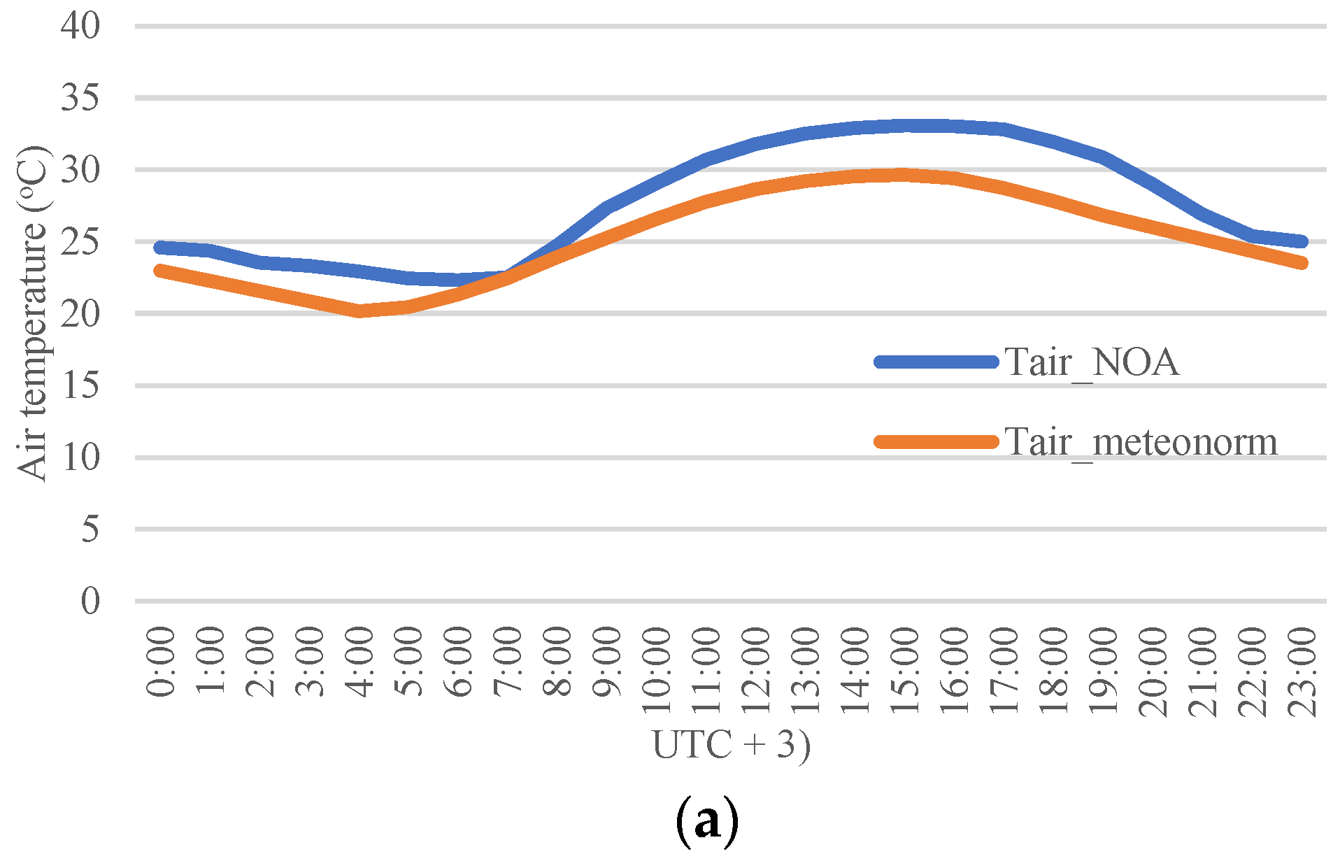
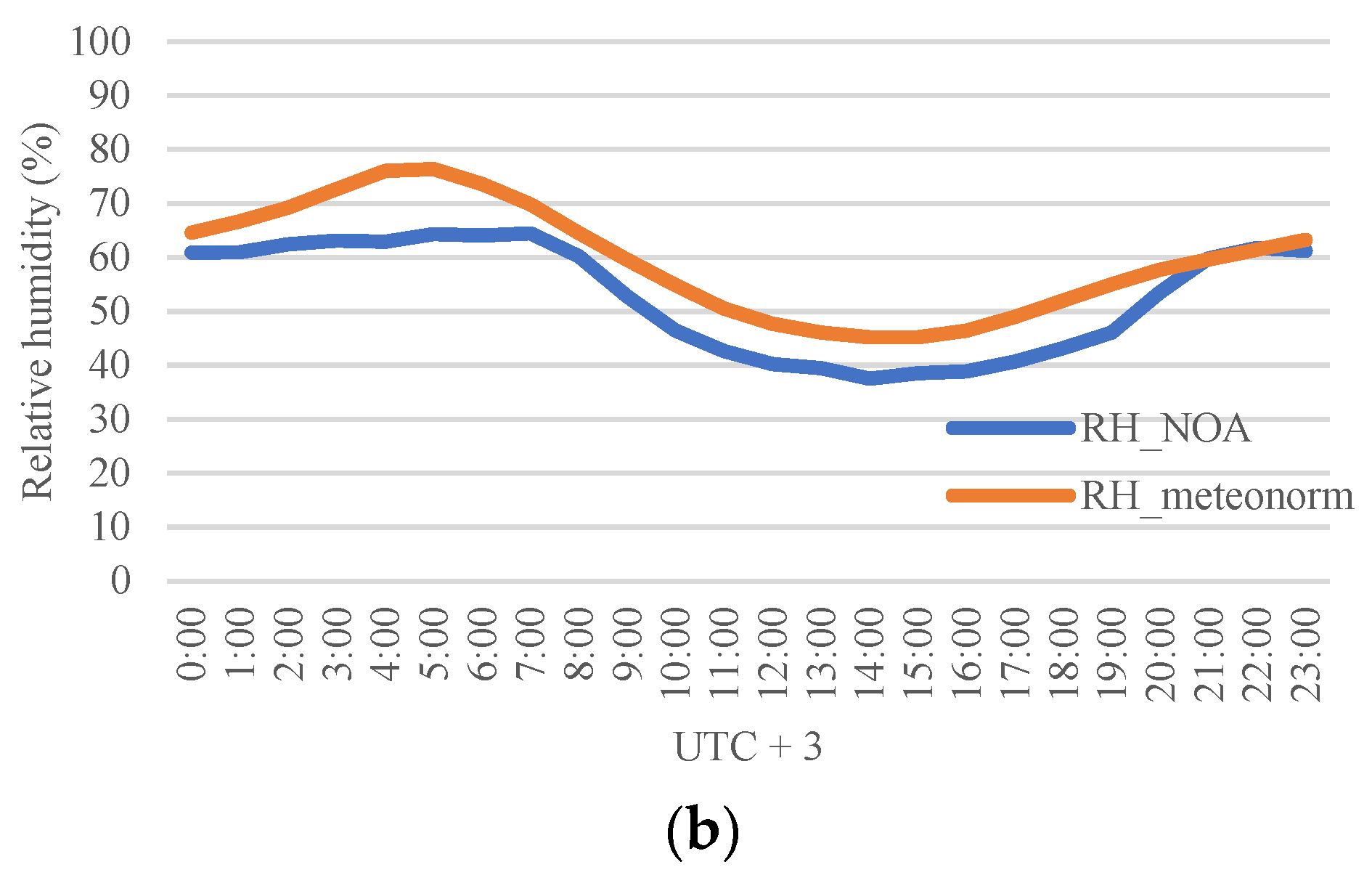
In summary, the site was characterized by high air temperature values and relatively low relative humidity and wind speed values. The air temperature may be affected to a great degree by the surrounded construction materials, as Tmrt values were also high (97.2 °C maximum and 47.1 °C average value). Furthermore, the absence of greenery was obvious, as predictable from the low values for relative humidity. These low values of humidity lead those of air temperature to extremely high levels, making in that way the region unbearable in terms of thermal comfort conditions. Finally, historical data (METEONORM V8) of both Tair and RH were also gathered and compared with those acquired from the NOA station. The comparison is presented in Figure 2a,b, which shows that the hourly average value of the air temperature in summer 2016 was equal to 27.6 °C, 2.4 °C above the average level (25.2 °C). Accordingly, the hourly average value of the relative humidity was found to be 6.7% lower than that recorded previously in the city of Xanthi (52.8% and 59.5%, respectively). The values that were observed in the city of Xanthi in the summer of 2016 may have played an important role in the existence of high values of air temperature that were observed in the field during the same measurement period.
3.2. Urban Heat Island
3.2.1. Canopy Urban Heat Island (CUHI)
A comparison of all measured microclimatic parameters between those experimentally measured and those gathered from the nearby meteorological station showed significant differences. Compared with that of the rural environment, the urban climate was found to vary in terms of air temperature, relative humidity, and wind speed. It must be pointed out, though, that the mobile station was placed inside the urban area and measured microclimatic parameters at a height of 1.5 m above ground. On the other hand, the meteorological station near the city of Xanthi measured the meteorological parameters at a height of 10 m. Therefore, the actual differences between the values at the location of the two sensors could be smaller if made at the same height. However, as it can be seen in Table 7, that despite the city of Xanthi not being considered a large urban area, it still differed greatly from suburban areas in terms of climate, and it can be stated that the urban heat island phenomenon was quite obvious in the city of Xanthi. According to Oke (1973) [1], “almost every urban environment through the world is from 1 °C to 4 °C warmer than neighbouring rural areas, and this enforcing urban heat island effect”. The urban heat island phenomenon is obvious in the city of Xanthi, as shown in Table 7. Therein, the average value of air temperature in the city of Xanthi is seen to be 4.6 °C higher than that of the region of Peteinos.
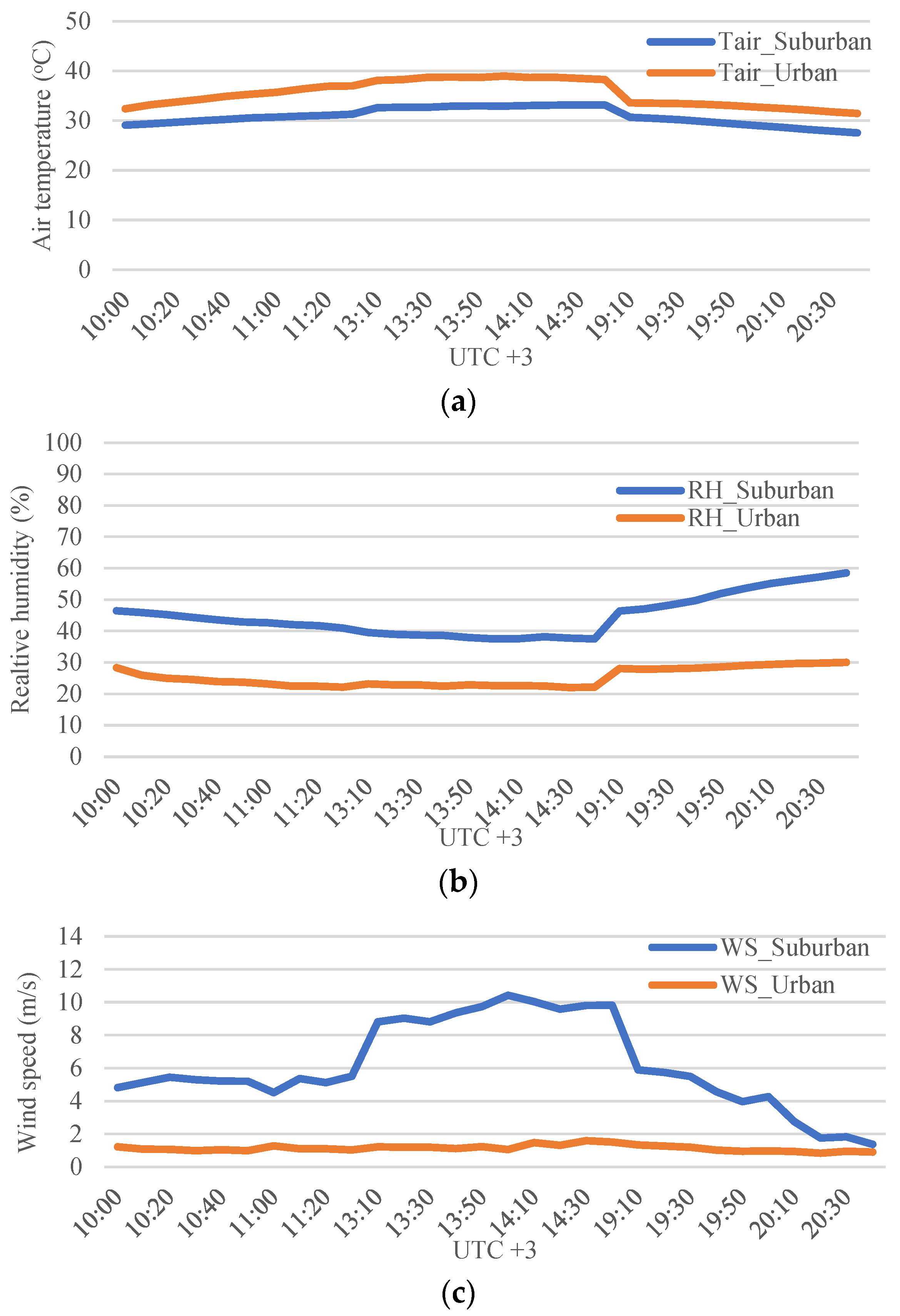
Significant differences appeared in all microclimatic data, as already mentioned. Concerning relative humidity, the average value in urban centres was 20.8% lower than that of the rural environment. This difference can be attributed to the lower level of vegetation and soil cover in the urban area of Xanthi compared to the larger area of greenery and natural landscapes in the region of Peteinos. While the meteorological station placed in the city of Xanthi was surrounded by buildings from 3 m to 21 m tall, the meteorological station of NOA was located in an open area with no obstacles surrounding it. This difference of morphology, led to great differences in terms of wind speed because the buildings provide obstacles to wind flow. Concerning solar radiation, no significant difference appeared between the two meteorological stations. The meteorological parameters are shown in Figure 3a–c. The outcomes indicate that both the morphology, the conventional structure material, and the absence of greenery play an important role concerning the intensity of the urban heat island in terms of CUHI.
3.2.2. Surface Urban Heat Island (SUHI)
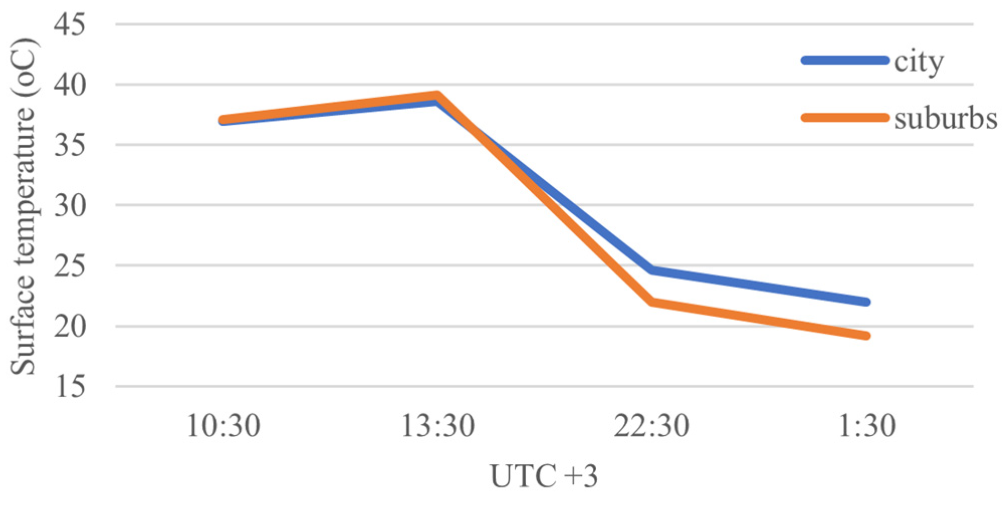
The urban heat island effect in terms of surface temperature was investigated by using remote sensing data. The satellite images contaminated with clouds, were removed. However, for the MODIS satellite, there were available data for almost all experimental days. Following the analysis of satellite images as described previously, the trend of the surface temperature for both the city and suburbs is presented in Figure 4. Significant differences appeared in terms of surface temperature between the city centre and the suburbs. More specifically, the average surface temperature inside the city core was 1.2 °C higher than that of the suburbs. The maximum difference between the city and suburbs in terms of ‘land surface temperature’ LST was 4.0 °C and appeared on 1 August 2016 at 22:34 UTC + 3. Figure 4 shows the greatest difference between the LST of the city and suburbs appeared at night. On the other hand, in the morning, the two temperatures were quite close and, in many cases, the LST of the suburbs was slightly higher than that inside the city core. This could be attributed to the properties of the construction materials inside the city. Constructive materials inside urban areas like pavements, roads, and buildings, can absorb large amount of heat from solar radiation. Therefore, during the night hours, the stored heat releases to the environment resulting in great differences in terms of temperature (both air and surface temperature) between urban environments and that of rural ones.
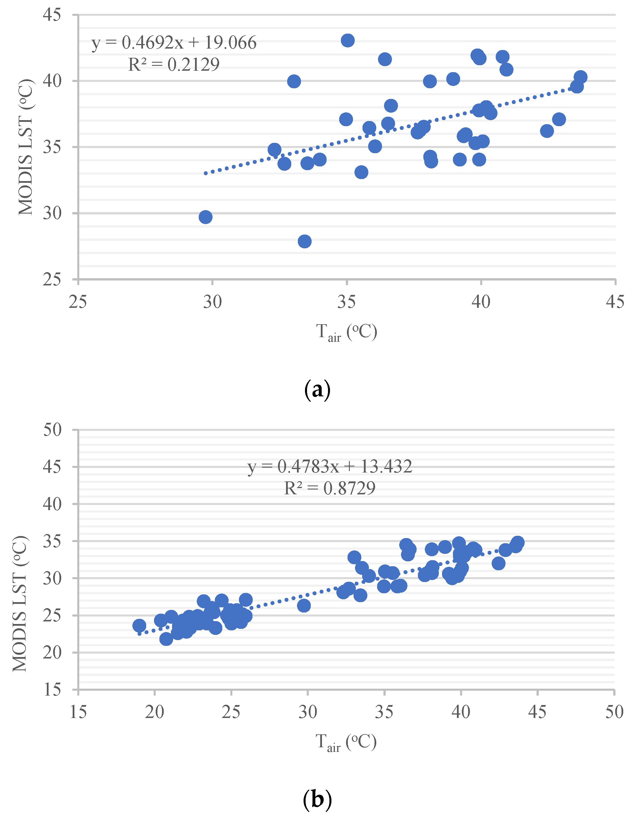
The relationship between the LST and Tair was also investigated. Quantifying air temperature as a function of surface temperature would be quite helpful for mapping air temperature in urban areas. In that way, hot spots in the urban environment would be easier to identify. For this reason, both Tair values and the available MODIS data were used in the investigation, and two tests were conducted. Firstly, Tair values that were gathered from the mobile station were compared with the LST data that were extracted from the MODIS images. Secondly, the Tair values that were gathered from the NOA station (Tair_met) were compared with the MODIS LST values. In Figure 5a,b, the correlation between the surface temperature and air temperature for the two tests is presented. This reveals in the first test a weak correlation (R2 = 0.21) between the MODIS LST and the Tair. However, concerning the second test, the correlation between the MODIS LST and the Tair_met can be described as strong (R2 = 0.87). Concerning the first test, the low correlation between the MODIS LST and the Tair data can be attributed to the low spatial resolution of the MODIS satellite (1000 m); this is a critical factor, as air temperature near the surface is more sensitive to different surface covers. For this reason, more satellite data are required for downscaling techniques to be applied and for the correlation between LST and Tair to be examined in more detail. Finally, because in situ measurements during the night hours were not performed, the correlation between the two parameters could only be performed for morning and afternoon hours. Concerning the second test, air temperature measured at higher levels (10 m above ground) were found to be predicted from satellite surface temperature data with relatively high accuracy. This may be attributed to the air temperature at higher levels not being affected to a great degree by the morphology of the ground, and therefore the low spatial resolution of MODIS satellite does not play an important role. The equation that described the relationship between air temperature and surface temperature is presented as follows:
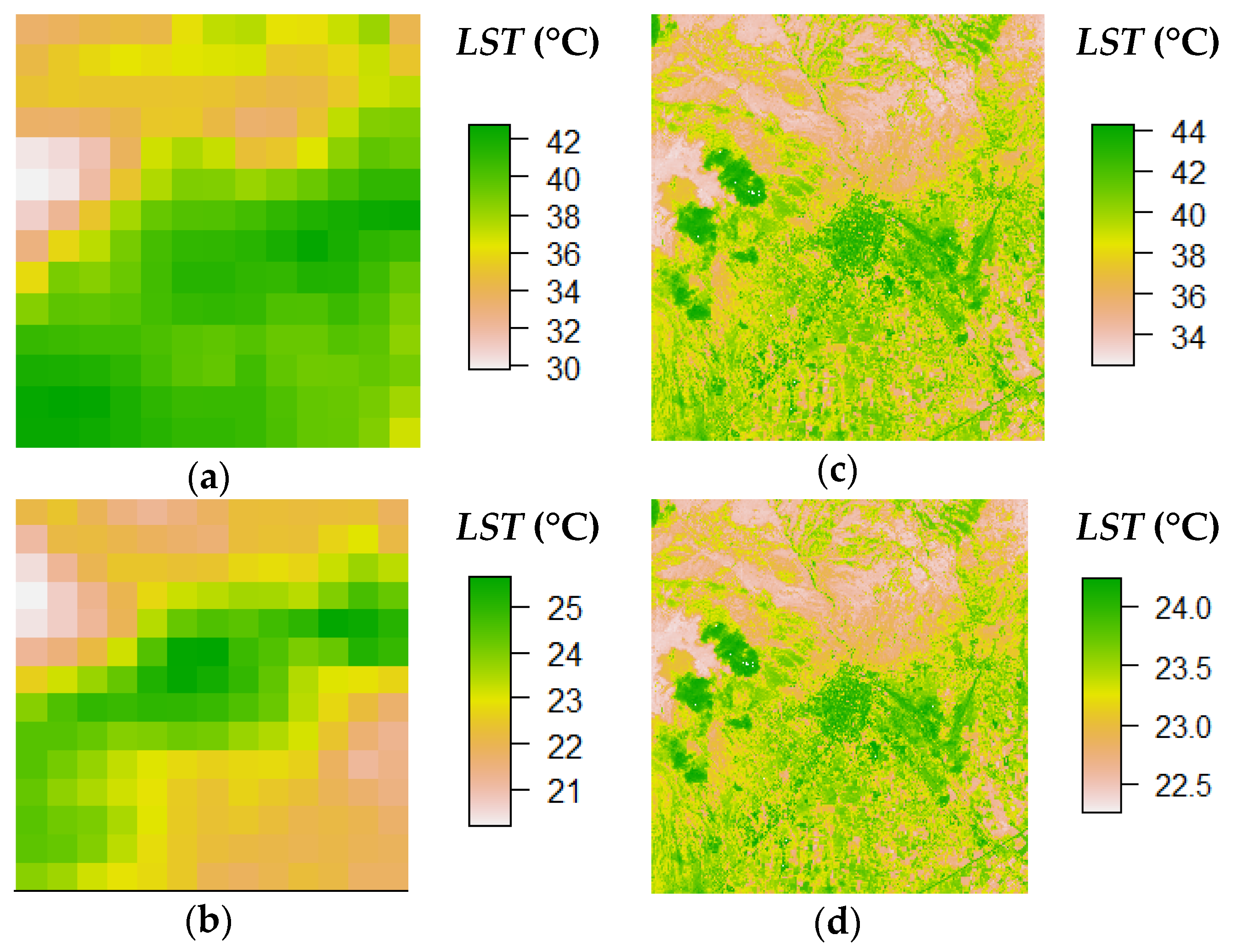
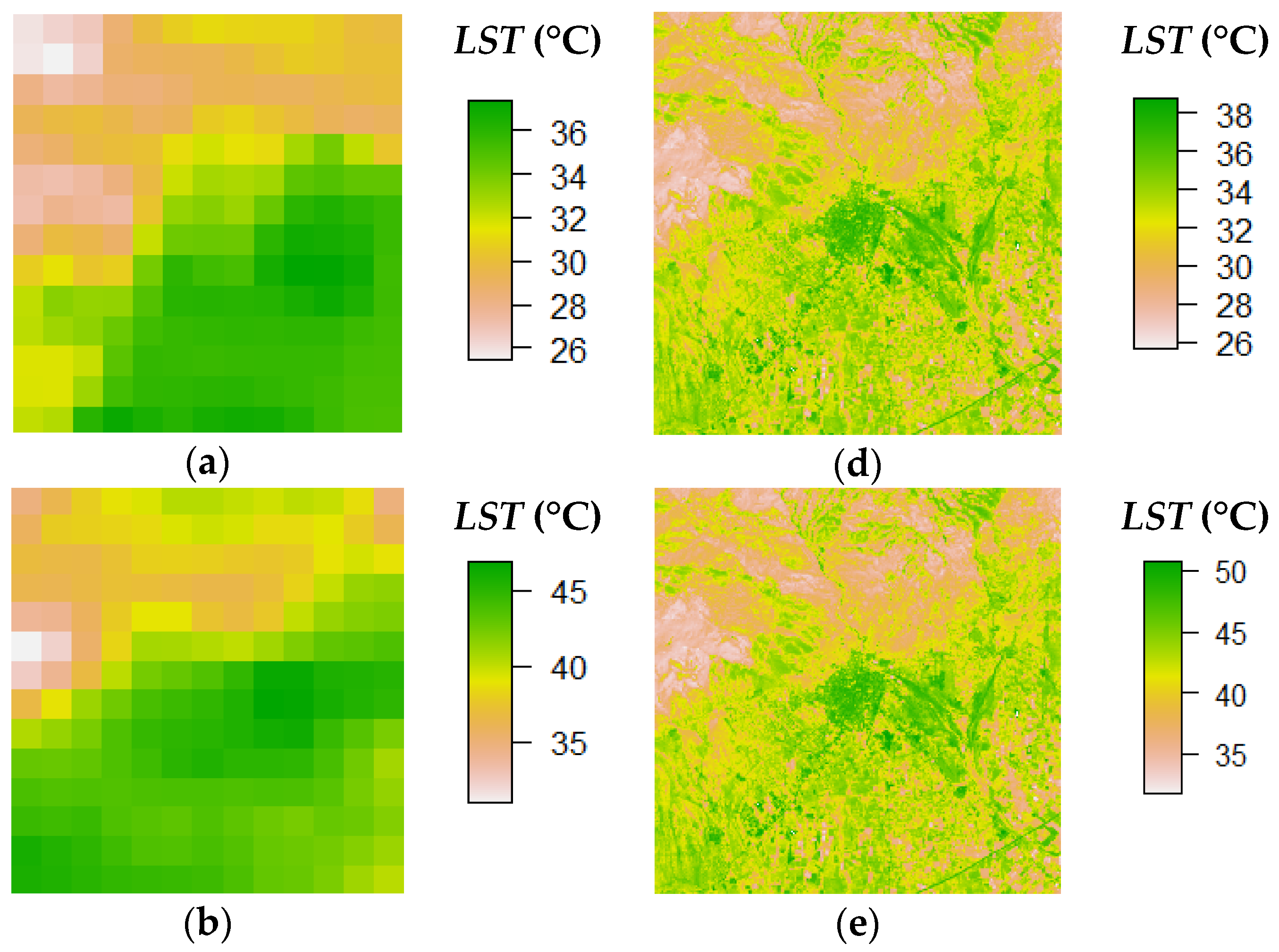
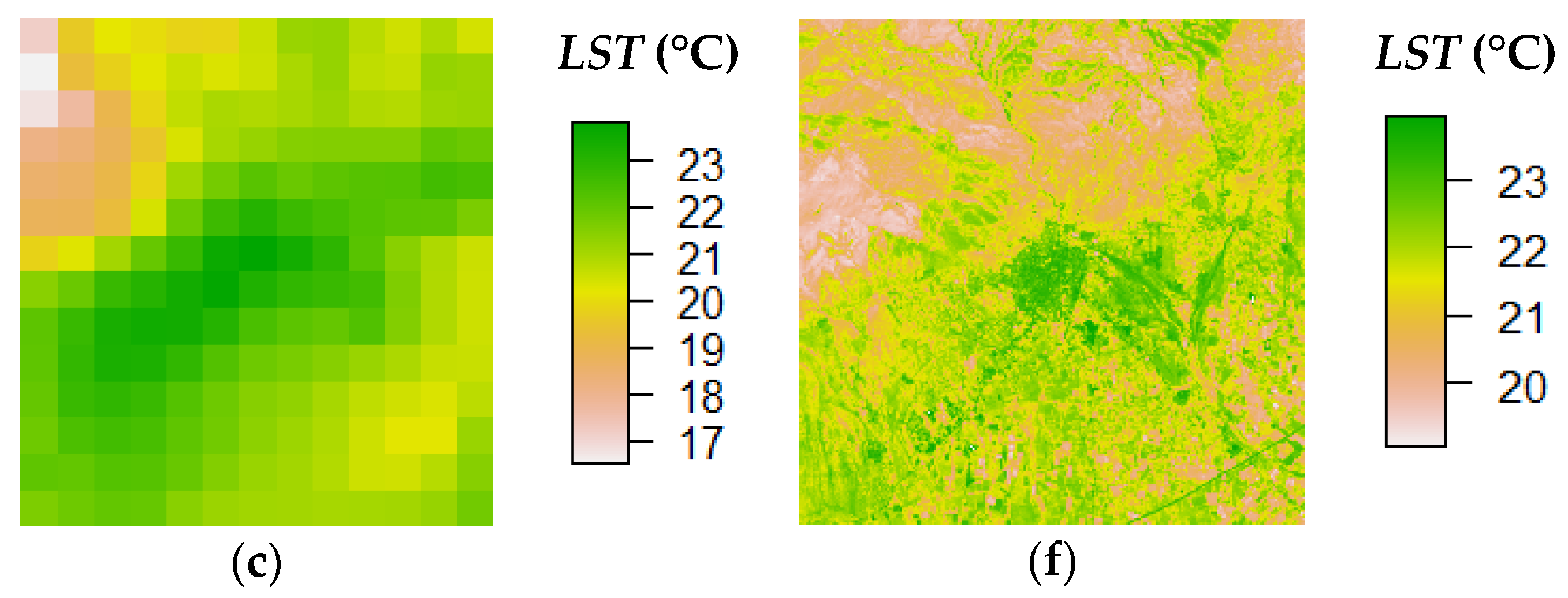
Finally, the TsHARP disaggregation method was applied to the different satellite data, as previously discussed. More specifically, thermal images were disaggregated from 1000 m, the initial spatial resolution of the MODIS, to 10 m (Sentinel-2) and 30 m (Landsat 8). Figure 6a,b shows the LST images with a spatial resolution of 1000 m and Figure 6c,d shows the corresponding downscaled LST images with spatial resolution of 10 m. Accordingly, Figure 7a,b shows the LST images with spatial resolution of 1000 m and Figure 7c,d shows the corresponding downscaled LST images with spatial resolution of 30 m. It is obvious from Figure 7 that the downscaled LST images offer more details for the spatial distribution of surface temperature in the region of interest. The temperature differences are obvious in the results, especially in the morning hours. In Table 8, the LST values in both the city and suburbs at a 1000 m and a 10 m spatial resolution are presented. Considering the downscaled images, the SUHI effect is more obvious in the morning hours, as the LST value inside the city core is 2.5 °C higher than that in the rural area at 11:35 UTC + 3. Even more obvious is the SUHI effect on 5 August 2016, Table 9, with the difference between the city and the suburbs, in terms of the surface temperature, equal to 6 °C. In contrast to what has already been described for the SUHI intensity concerning the MODIS LST 1000 m data, in the case of both the MODIS LST 10 m and the MODIS LST 30 m, on both days the SUHI intensity was more obvious in the morning and afternoon hours.
3.3. Questionnaire Data
Totally, 266 questionnaires were dispersed, 30% of interviews took place from 10:00 to 11:30, 54% took place from 13:10 to 14:40, and 16% from 19:10 to 20:40. This difference is reasonable, because there are a lot of people who visit the coffee restaurants and the shopping centres in the morning and in the afternoon. On the other hand, the area becomes less crowded the evening hours.
Of the interviewees, 52% were males, 40% visited the site for entertainment, and about 20% for work. These results are quite reasonable because the study area is a shopping street and has a lot of coffee restaurants. Therefore, most visitors are people who use the site for recreational purposes or they are employees. Additionally, most of the sample were city residents (62.8%).
Regarding age, 90.23% of the sample were 18 to 54 years old, and 33.5% of them were aged between 25 and 34 years, which was thus the most frequent age group. Finally, the clothing thermal insulation ICL of people ranged between 0.3 to 1.2 clo, with the mean value equal to 0.4 clo. Table 10 summarizes the average values for weather data, clothing insulation and the age of the respondents for the comfort values of the questionnaires.
According to the microclimatic monitoring performed in the area and the assessment of all questionnaires, people perceived thermal comfort at a mean air temperature of 33.7 °C.
3.3.1. Actual Sensation Vote (ASV)
Responses from people interviewed during the survey showed that the perceived thermal comfort (Actual Sensation Vote, ASV) covered only three vote point scales of the five points available. The percentage of responses was 54.1% for comfort, 30.1% for slightly warm, and 15.8% for very warm.
To assess which factor was related to thermal comfort, the parameters were divided into the following categories: meteorological, personal, and physiological.
3.3.2. Actual Sensation and Weather Parameters
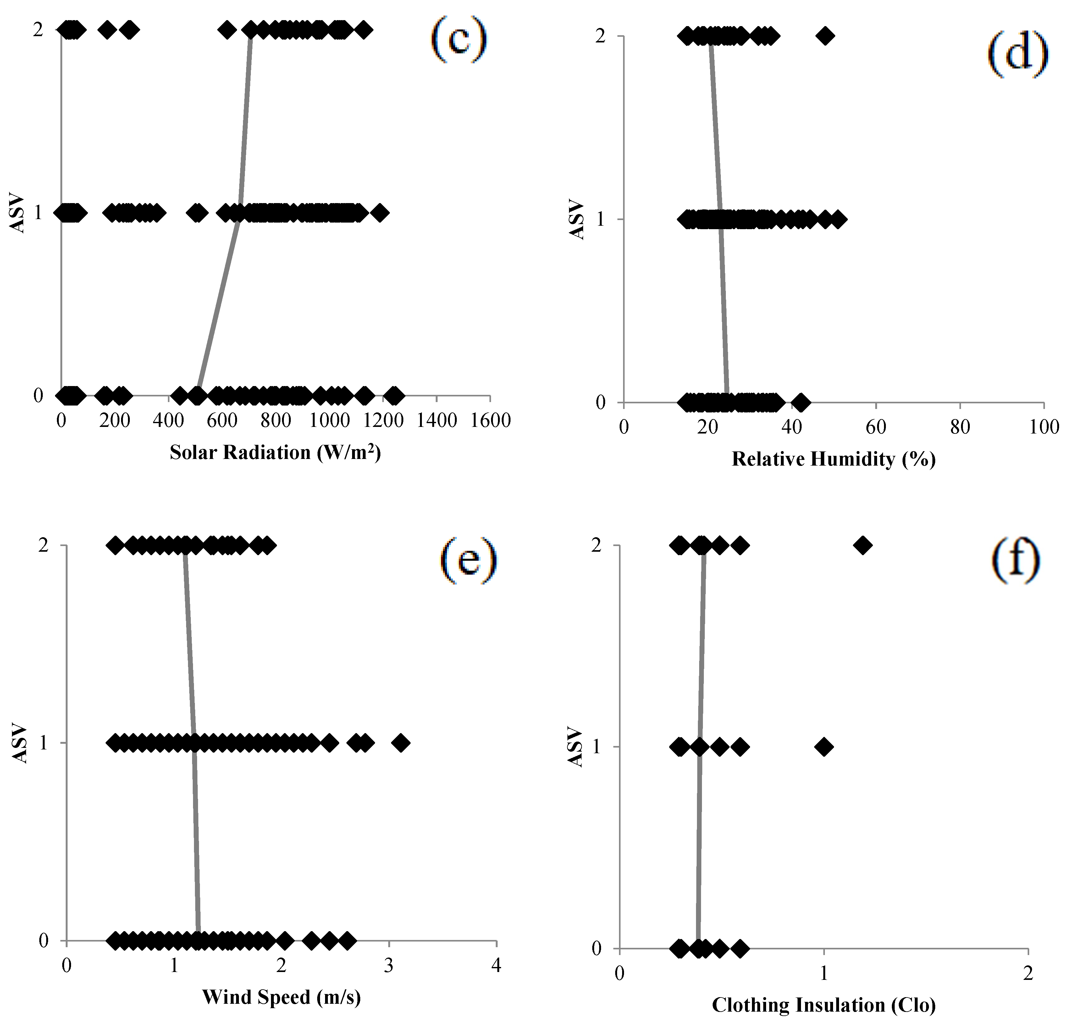
One-way ANOVA was applied at the data, and it was shown that there was a significant difference between the classes of ASV and all the weather parameters, except for wind speed. Additionally, a Tukey post-hoc test was applied at the data to examine the statistically important differences between the examined parameters. The Tukey post-hoc test revealed statistically important differences between all ASV levels and averages in the cases of Tair and Tmrt. In the case of Tmrt, the analysis revealed statistically significant differences only for the ASV level from 0 and 1. For the solar radiation, the Tukey post-hoc analyses showed statistically significant differences only for the ASV level between 0 and 1, and for relative humidity only for the level between 1 and 2. Finally, in the case of wind speed, no significance was observed in the different levels of ASV.
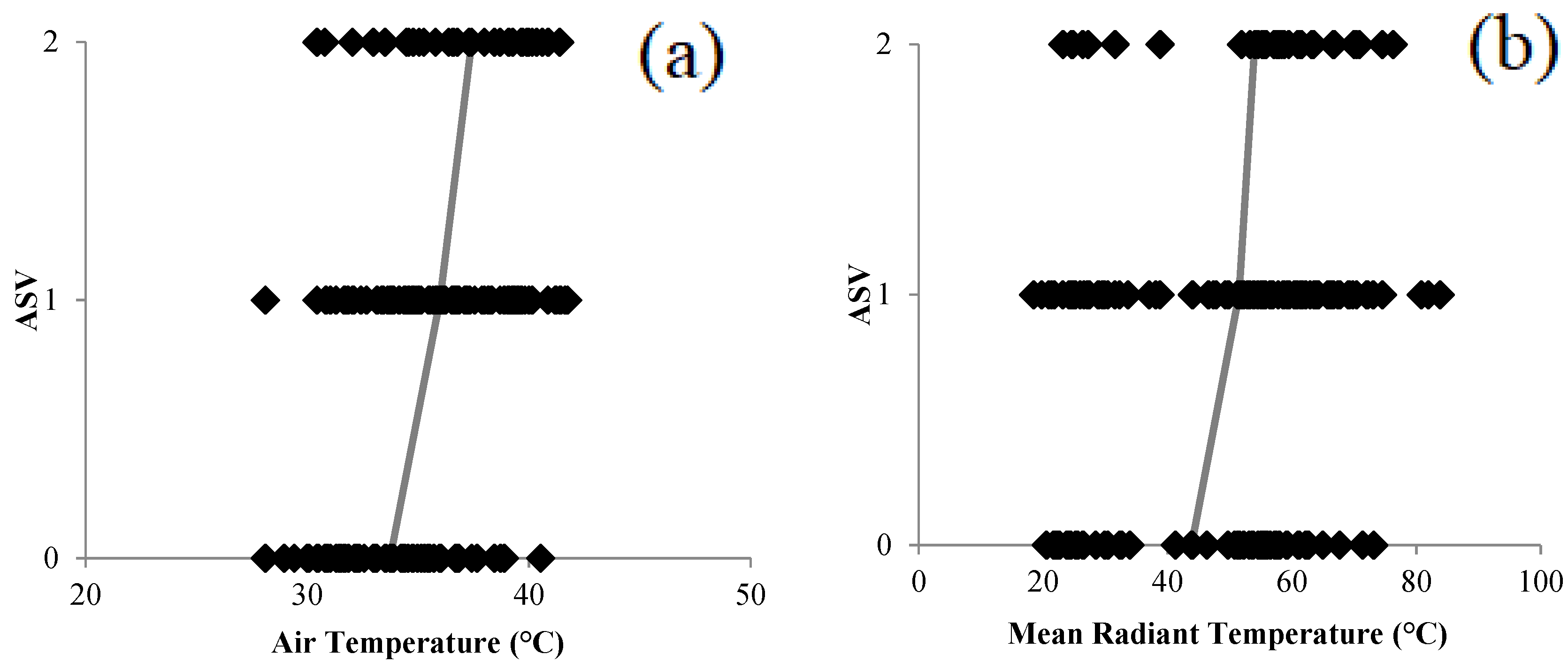
The statistical analysis showed that the value group for air temperature during summer at which people felt comfortable was between 33.7 and 36 °C, while the standard deviation between categories 1 and 2 decreased about 1.4 °C. These results are quite close with those from previous studies performed in Greece [75]. In the case of the mean radian temperature, higher differences between all classes were observed, showing the importance of radiation. In Figure 8a–f, the weather parameters and clothing insulation per level of Actual Sensation Vote (ASV) are presented.
3.3.3. Actual Sensation and Personal Characteristics
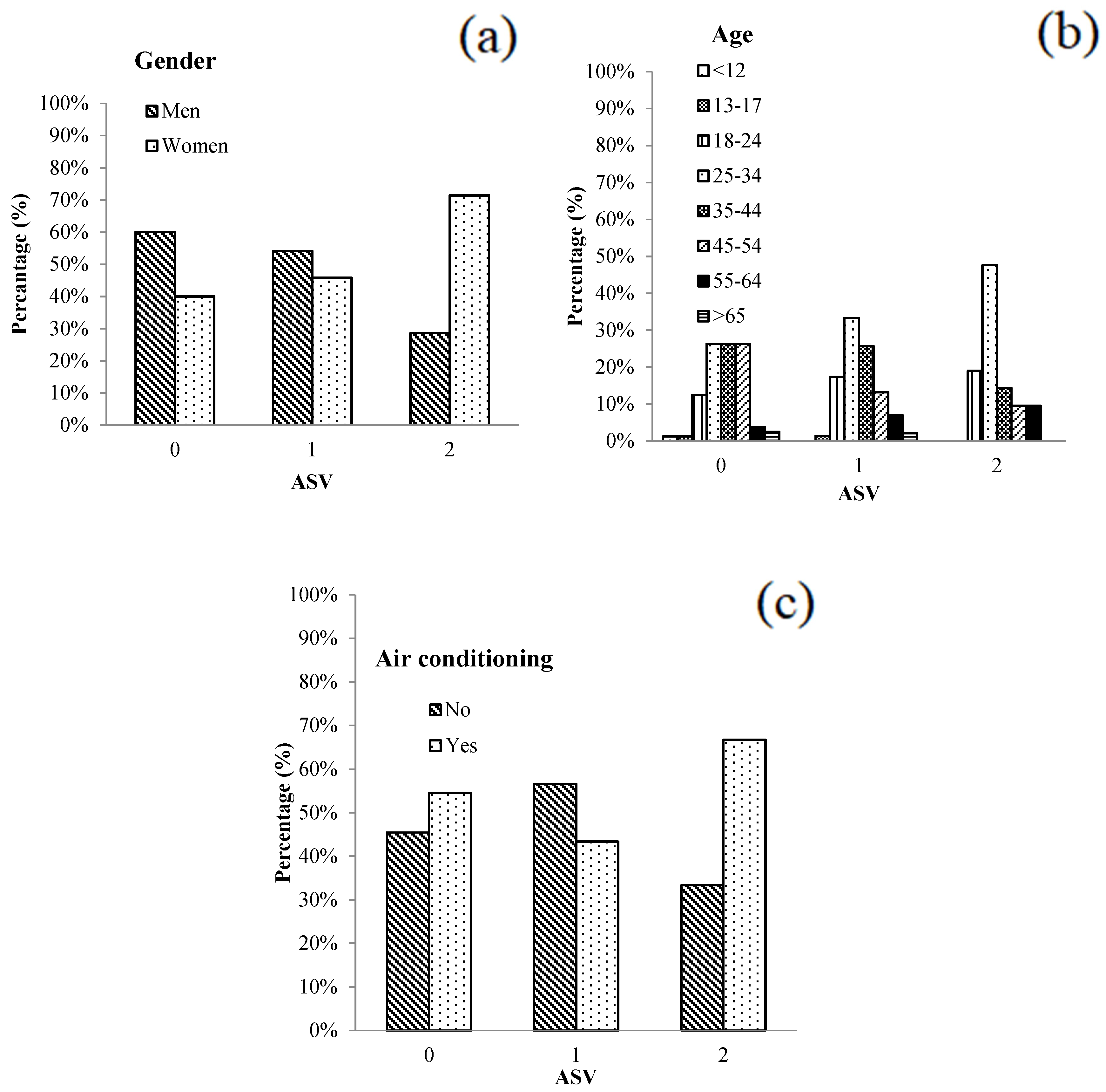
The responses showed that women felt warmer than men. More specifically, a higher percentage of ASV in the level of 0 (comfort) was observed in males (60%). Furthermore, a higher percentage in the level of 1 (slightly warm) was observed in men (54.2%) compared to women (45.8%). In the level of 2 (very warm), a quite high percentage of actual sensation votes was observed in females (71.4%) than in men (28.6%).
Vulnerability to heat was observed for people in the age of 18 to 34 years and people between 55 and 64 years. Additionally, the interviewers who previously were in a conditioned place tended to vote the extreme class on the actual sensation scale. In Figure 9, the personal parameters per class of the Actual Sensation Vote (ASV) are presented.
3.4. Actual Sensation and Physiological Factors
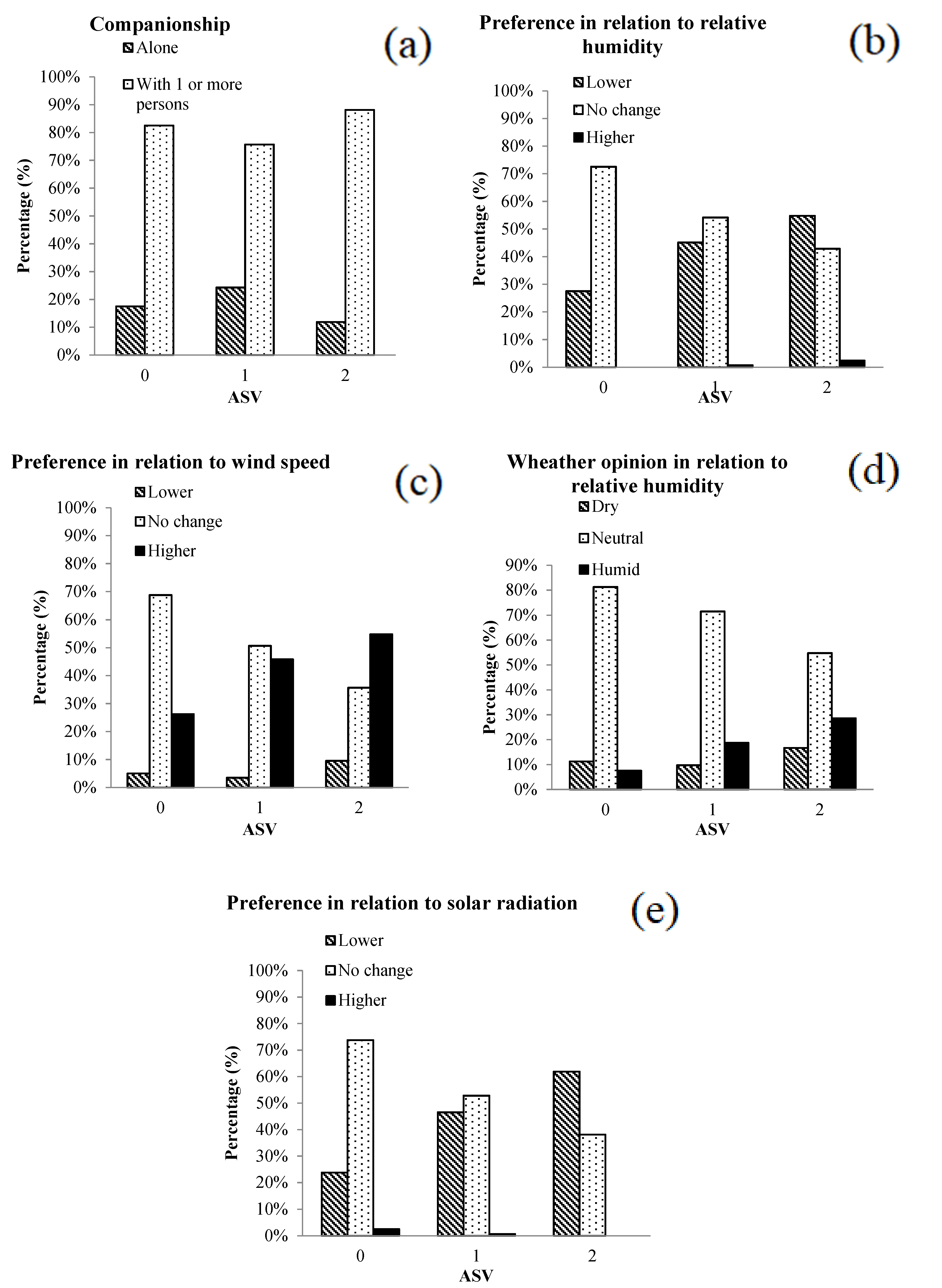
Actual sensation is dependent on companionship and total comfort. A great number of votes (88.1%) in the higher level of the ASV scale (very warm) was observed among persons who were with companionship during the interview in comparison with those who were alone (11.9%).
Most respondents (73.8%) who felt comfortable stated that the site was comfortable. Accordingly, most respondents who felt very warm (90.5%) stated that they preferred cooler thermal environments. In relation to the weather opinion, most respondents who felt comfortable stated that the day of the interview was warm, with normal levels of humidity and solar radiation, and low wind velocity. Concerning the level of solar radiation, we must underline that most people who participated in the interview (95%) were in a shaded place and as a matter of fact were not affected by the solar radiation.
Regarding the preference for microclimatic conditions, people who felt very warm, stated that they preferred lower levels of relative humidity (54.8%) and solar radiation (61.9%) and a higher level of wind velocity (54.8%). In Figure 10a–e, the psychological parameters per class of the Actual Sensation Vote are presented.
3.5. Actual Sensation Prediction
To investigate which parameter was the most important for thermal sensation, an ordinal regression analysis was applied at the data. The Tmrt values were excluded from the analysis because they were highly correlated to the Tair values. Air temperature was selected instead of Tmrt for the analysis because it is measured with high accuracy and there is no need of applying further equations for its calculation. All meteorological parameters were found to be statistically significant (<0.05), apart from the wind speed. According to the ordinal regression analysis, the ASV was not correlated with shading, visit purpose, place of birth, frequency of visiting, consumption (drink or food), companionship and clothing insulation. The most statistical important weather parameters were the Tair and SR (Table 11).
Among respondents, women felt warmer than men. Furthermore, people aged from 25 to 34 and 55 to 64 years felt warmer than those who belonged to the remaining age groups. Finally, regarding psychological factors, the ASV was significantly correlated with both the respondents’ opinion about weather conditions and their preference for all different microclimatic parameters. According to this analysis, people felt comfort in relation to relative humidity and solar radiation and felt warm in relation to air temperature. Furthermore, most respondents felt that the level of wind speed was low. In relation to preference, people preferred lower air temperature. Regarding relative humidity, wind speed and solar radiation, most respondents did not prefer any change (Figure 7).
3.6. Subjective and Objective Thermal Sensation
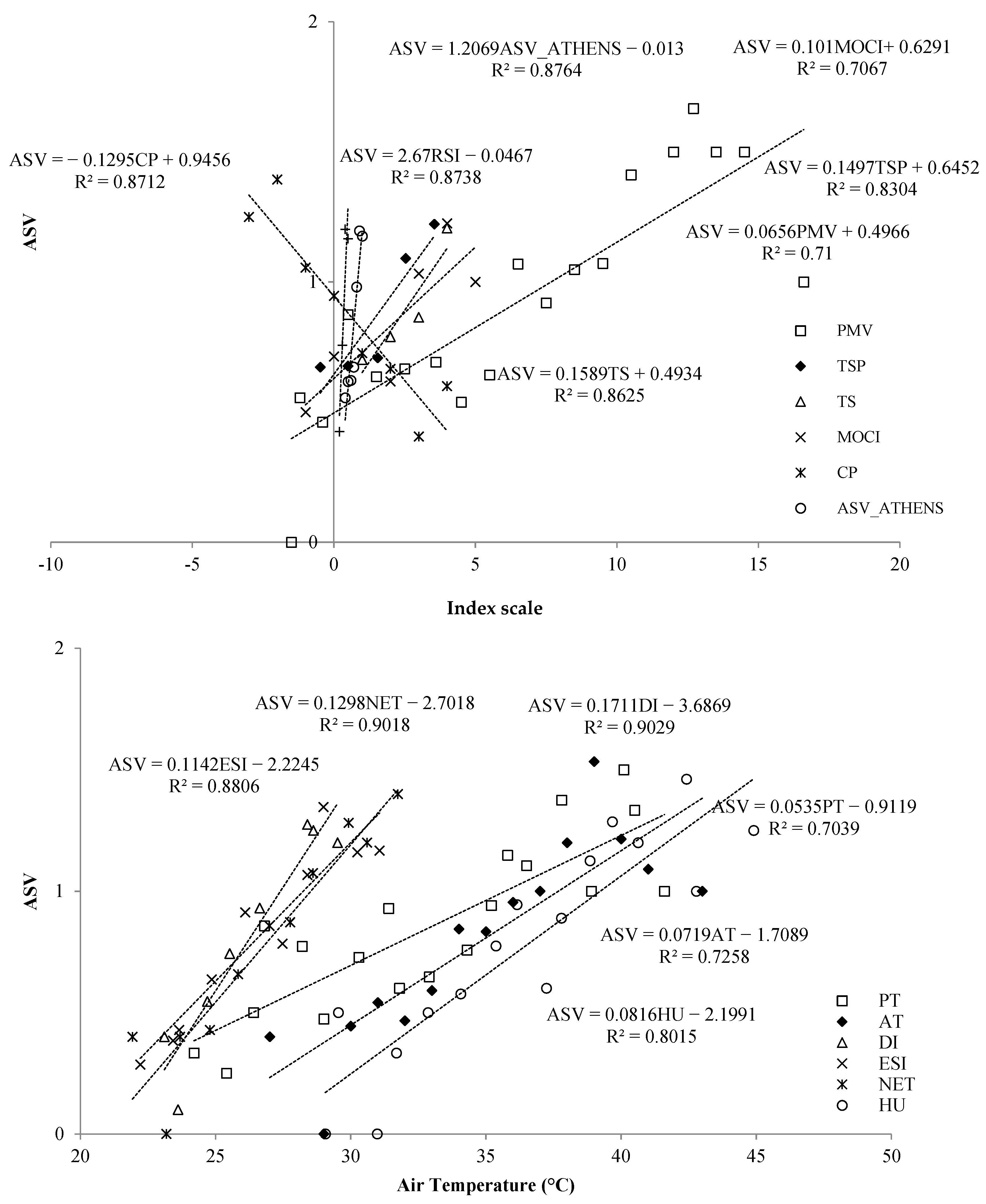
As shown in Figure 11, among all ‘rational indices’, the PMV (Equation (24)) and PT (Equation (25)) were found to be the indices with strong correlation with the ASV, having similar ability to predict comfort votes, but the PMV had the strongest correlation (Equation (23)) with R2 = 0.71.
The results are concordant with other studies in Mediterranean regions [72]. The rest of ‘rational indices’ cannot describe the comfort votes. Concerning the ‘empirical indices’, apart from the WBGT, all had strong correlation with the ‘Actual Sensation Vote’ (ASV). The ASVATHENS was found to be the most appropriate one with the implication of the model (Equation (26)):
Finally, most of the indices based on linear equations showed strong correlation between Actual Sensation Vote. The DI and NET were found to be the more appropriate indices to describe the comfort votes in the city of Xanthi in summer conditions with the implication of the models (Equation (27) and Equation (28) respectively):
3.7. City Comfort Index
Several ASV models for the city of Xanthi were investigated based on the collected climatic data and people questionnaire responses. The ASV equation takes into consideration four microclimatic parameters: air temperature, solar radiation, wind speed and relative humidity. Different climatic data sources were tested for the calculation of the ASV, and the most effective model was selected. The questionnaires were randomly collected in time and thus, the in situ measurements from the mobile meteorological station had very short time intervals (every 1 min) allowing for better correspondence with the interview time, while the nearby city meteorological station monitors data every 10 min.
In the first approach, the regression model was calculated with the in situ climatic measurement data. To compare the ASV model with the one derived from the meteorological station data, questionnaire responses corresponding to 10 min time steps were selected for the analysis. Due to this procedure, the examined questionnaire responses dropped from 266 to 165. The regression model concerning in situ measurements was calculated as:
The same procedure used previously was followed with data collected from the nearby meteorological station. The regression model is described as:
Another regression model was investigated based on all in situ monitored climatic data and questionnaire responses and thus, considering all 266 observations (all collected questionnaires) and is described as follows:
For the examination of the ASV model based on all questionnaire responses and meteorological station data, an interpolation between consequent 10 min data was done to derive a value for the time of the questionnaire interview. The regression model is described as follows:
In all examined cases, the correlation coefficient was found to be in line with previous studies (0.26 to 0.68) [71], or between 0.41 and 0.46. Minor differences, though, appeared among all regression models. The most sufficient regression model was found to be the one that took into consideration the meteorological parameters gathered from the nearby station that monitored data every 10 min (r = 0.46) and the reduced number of questionnaires corresponding at the meteorological recording time. On the other hand, the most insufficient was found to be the one that also took into consideration the microclimatic parameters gathered from the nearby station and included all questionnaires. This procedure, by narrowing the gap with closer values, led to uncertainties as some microclimatic parameters were very unstable and unpredictable (especially solar radiation due to cloud effect and wind speed) making this procedure less valid.
4. Conclusions
- ➢
- The area of interest was characterized by high values of air temperature and low values of relative humidity and wind speed.
- ➢
- The urban heat island effect was obvious in the city of Xanthi, especially in the morning and afternoon, as the average air temperature inside the city core was found to be 4.6 °C higher than that of the rural area of Peteinos.
- ➢
- The absence of greenery and morphology of the site of interest play an important role for the existence of the urban heat island effect.
- ➢
- The average surface temperature inside the city core was 1.2 °C higher than that of the suburbs. The maximum difference was found to be equal to 4.0 °C.
- ➢
- A strong correlation was found between the MODIS LST (1000 m spatial resolution) and the air temperature derived from the nearby meteorological station (10 m above ground). Low spatial resolution of satellite data plays an important role for the air temperature at the lower levels to be quantified.
- ➢
- Taking into consideration pan-sharpened images of 10 m and 30 m spatial resolution, the intensity of the SUHI effect was also more obvious in the morning and afternoon.
- ➢
- Concerning the thermal sensation assessment, both air temperature and solar radiation were found to be significant parameters.
- ➢
- As for subjective and objective thermal sensations were concerned, most of the direct indices described the comfort votes well.
- ➢
- A model that predicted thermal comfort inside the city core of Xanthi was found. This model considered weather parameters from the nearby meteorological station.
5. Discussion
A lot of focus has been given to large urban areas globally and less to small towns or medium scale cities. The current work focused on the assessment of the urban heat island effect in a medium-sized Mediterranean city. In terms of CUHI, the intensity of the urban heat island effect exceeded 4 °C. Concerning SUHI, the urban heat island effect was found to be equal to 4 °C in the case of non-pansharpened images and equal to 6 °C in the case of downscaled images (Landsat8, 30 m). The urban heat island effect, in terms of SUHI, might be even more intensive considering that many surfaces cannot be accounted for due to spatial resolution limitation. Furthermore, due to the temporal frequency of the MODIS images, many hours during the day cannot be investigated. What can be concluded, is that the morphology of the area of interest, as well as the absence of greenery, has an important role concerning microclimate effects. Additionally, the thermal properties of the conventional materials that covered both buildings and pavement may be another significant factor. Nevertheless, the correlation between air temperature acquired from the nearby meteorological station and surface temperature acquired from the MODIS satellite at 1000 m spatial resolution was found to be strong. On the other hand, the linear relationship between the MODIS LST and air temperature that was measured in the study area was found to be weak. However, the relationship between land surface temperature from satellites and air temperature at lower levels (1.5 m above ground) is also necessary for mapping air temperature inside medium scale cities at higher resolution. For this reason, more satellite data are required for downscaling techniques to be performed and measurements acquired during the night are necessary for more reliable results.
Concerning the thermal comfort assessment, and more specifically Actual sensation and weather parameters, the statistical procedure showed a significant difference between levels of actual sensation vote and weather parameters, except for wind speed. For the mean radiant temperature (Tmrt), Tukey post-hoc analyses showed significant differences only for ASV levels 0 and 1, for the solar radiation only for ASV levels 0 and 1, and finally for the relative humidity, only for the level between 1 and 2. Concerning actual sensation prediction, ordinal regression showed that all meteorological factors were statistically important except wind speed. As previous studies that have been conducted in large cities have already shown, and as in the case of the city of Xanthi, the most significant parameters are the air temperature and the solar radiation [72].
Concerning subjective and objective thermal sensations, the empirical and the direct indices described the comfort votes well. More specifically, the DI and NET were found to be highly correlated with ASV (R2 = 0.90). The CP index has been already applied with success in many projects in Greece [96,97] and according to our research was evaluated as one of the most appropriate thermo-physiological indices (R2 = 0.87). Among the empirical indices, almost all showed strong correlations with R2 values higher than 0.70. In contrast, the WBGT as previous studies have already shown, do not reflect in a great degree the vote for comfort of the interviews [72]. Finally, among rational indices, only the PMV and PT were found to be appropriate to describe the comfort votes, with R2 values equal to 0.71 and 0.70, respectively. As previous studies in Mediterranean climates [72] have already shown, the OUT_SET index is directly affected by the solar environment and for this reason is quite unstable and, therefore, is not able to describe comfort votes. Furthermore, the PET is affected to a great degree by the air temperature and as a result cannot describe comfort votes especially in summer.
Finally, an attempt to derive a city comfort index (ASV) was made using different climatic data and number of questionnaires. The regression models were compared with those that were calculated in previous studies. All regression models were quite close in terms of the regression coefficient. However, the regression model that considered the microclimatic parameters acquired from the nearby meteorological station with data every 10 min, showed the highest regression coefficient, providing in that way an index that can predict thermal comfort conditions for the city of Xanthi during summer.
The outcomes of the current study, underline the fact that medium scale cities need more attention to be comfortable regarding thermal sensation. Furthermore, many thermal comfort results were found to be in accordance with those derived from previous studies that were conducted in large urban areas showing that medium scale cities act like large urban environments, and that more studies should be conducted in medium scale cities in the future.
Author Contributions
Conceptualization, G.K. and A.D.; Methodology, G.K. and A.D.; Software, G.K., A.D. and S.Z.; Validation, G.K., A.D., P.T. and S.Z.; Investigation, G.K. and A.D.; Writing—Original Draft, G.K. and A.D.; Writing—Review & Editing, G.K., A.D., P.T. and S.Z.; Visualization, G.K.; Supervision, A.D.; Project administration, A.D.; Monitoring, G.K, A.D. and P.T. All authors have read and agreed to the published version of the manuscript.
Funding
This research received no external funding.
Institutional Review Board Statement
Not applicable.
Informed Consent Statement
Not applicable.
Data Availability Statement
Not applicable.
Acknowledgments
This work was based on data collected during the dissertation thesis carried out in the frame of the Master of Science course ‘Environmental Engineering and Science’, at the Department of Environmental Engineering, Democritus University of Thrace, Greece.
Conflicts of Interest
The authors decleare no conflict of interest.
Appendix A
The questionnaire used in the current study.

References
- Oke, T.R. City size and the urban heat island. Atmos. Environ. 1973, 7, 769–779. [Google Scholar] [CrossRef]
- Anbar, M. The Climate Impact on Human Comfort in the Eastern Nile Delta; Cairo University: Cairo, Egypt, 2012; pp. 267–319. [Google Scholar]
- Oke, T.R.; Mills, G.; Christen, A.; Voogt, J. Urban Climates; Cambridge University Press: Cambridge, UK, 2017. [Google Scholar]
- Voogt, J.A.; Oke, T.R. Thermal remote sensing of urban climates. Remote Sens. Environ. 2003, 86, 370–384. [Google Scholar] [CrossRef]
- Bottyán, Z.; Kircsi, A.; Szegedi, S.; Unger, J. The relationship between built-up areas and the spatial development of the mean maximum urban heat island in Debrecen, Hungary. Int. J. Climatol. 2005, 25, 405–418. [Google Scholar] [CrossRef] [Green Version]
- Bottyán, Z.; Unger, J. A multiple linear statistical model for estimating the mean maximum urban heat island. Theor. Appl. Climatol. 2003, 75, 233–243. [Google Scholar] [CrossRef]
- Bruse, M.; Fleer, H. Simulating surface–plant–air interactions inside urban environments with a three dimensional numerical model. Environ. Model. Softw. 1998, 13, 373–384. [Google Scholar] [CrossRef]
- Bruse, M. ENVI-met 4. Available online: http://www.envi-met.info (accessed on 9 March 2021).
- Dimoudi, A.; Zoras, S.; Kantzioura, A.; Stogiannou, X.; Kosmopoulos, P.; Pallas, C. Use of cool materials and other bioclimatic interventions in outdoor places in order to mitigate the urban heat island in a medium size city in Greece. Sustain. Cities Soc. 2014, 13, 89–96. [Google Scholar] [CrossRef]
- Camilloni, I.; Barros, V. On the Urban Heat Island Effect Dependence on Temperature Trends. Clim. Change 1997, 37, 665–681. [Google Scholar] [CrossRef]
- Stewart, I.D.; Oke, T.R. Local Climate Zones for Urban Temperature Studies. Bull. Am. Meteorol. Soc. 2012, 93, 1879–1900. [Google Scholar] [CrossRef]
- Arnfield, A.J. Two decades of urban climate research: A review of turbulence, exchanges of energy and water, and the urban heat island. Int. J. Climatol. 2003, 23, 1–26. [Google Scholar] [CrossRef]
- Gedzelman, S.D.; Austin, S.; Cermak, R.; Stefano, N.; Partridge, S.; Quesenberry, S.; Robinson, D.A. Mesoscale aspects of the Urban Heat Island around New York City. Theor. Appl. Climatol. 2003, 75, 29–42. [Google Scholar] [CrossRef]
- Chen, X.L.; Zhao, H.M.; Li, P.X.; Yin, Z.Y. Remote sensing image-based analysis of the relationship between urban heat island and land use/cover changes. Remote Sens. Environ. 2006, 104, 133–146. [Google Scholar] [CrossRef]
- Hu, Y.; Jia, G. Influence of land use change on urban heat island derived from multi-sensor data. Int. J. Climatol. 2010, 30, 1382–1395. [Google Scholar] [CrossRef]
- Weng, Q.; Lu, D.; Schubring, J. Estimation of land surface temperature–vegetation abundance relationship for urban heat island studies. Remote Sens. Environ. 2004, 89, 467–483. [Google Scholar] [CrossRef]
- Pongrácz, R.; Bartholy, J.; Dezső, Z. Application of remotely sensed thermal information to urban climatology of Central European cities. Phys. Chem. Earth Parts A/B/C 2010, 35, 95–99. [Google Scholar] [CrossRef]
- Weng, Q. Thermal infrared remote sensing for urban climate and environmental studies: Methods, applications, and trends. ISPRS J. Photogramm. Remote Sens. 2009, 64, 335–344. [Google Scholar] [CrossRef]
- Martin, M.; Chong, A.; Biljecki, F.; Miller, C. Infrared thermography in the built environment: A multi-scale review. Renew. Sustain. Energy Rev. 2022, 165, 112540. [Google Scholar] [CrossRef]
- Tejedor, B.; Lucchi, E.; Nardi, I. Application of Qualitative and Quantitative Infrared Thermography at Urban Level: Potential and Limitations. In New Technologies in Building and Construction; Springer: Singapore, 2022; Volume 258, pp. 3–19. [Google Scholar] [CrossRef]
- ANSI/ASHRAE Standard 55–2013; Thermal Environmental Conditions for Human OccupancyAmerican Society of Heating, Refrigerating and Air-Conditioning Engineers. American Society of Heating, Refrigerating and Air-Conditioning Engineers: Atlanta, GA, USA, 2013.
- Fang, Z.; Feng, X.; Liu, J.; Lin, Z.; Mak, C.M.; Niu, J.; Tse, K.-T.; Xu, X. Investigation into the differences among several outdoor thermal comfort indices against field survey in subtropics. Sustain. Cities Soc. 2019, 44, 676–690. [Google Scholar] [CrossRef]
- Cheng, Y.; Niu, J.; Gao, N. Thermal comfort models: A review and numerical investigation. Build. Environ. 2012, 47, 13–22. [Google Scholar] [CrossRef]
- Fanger, P.O. Thermal Comfort. Analysis and Application in Environmental Engineering, 1st ed.; Danish Technical Press: New York, NY, USA, 1970. [Google Scholar]
- Jendritzky, G.; Nübler, W. A model analysing the urban thermal environment in physiologically significant terms. Meteorol. Atmos. Phys. 1981, 29, 313–326. [Google Scholar] [CrossRef]
- Gao, S.; Li, Y.; Wang, Y.A.; Meng, X.Z.; Zhang, L.Y.; Yang, C.; Jin, L.W. A human thermal balance based evaluation of thermal comfort subject to radiant cooling system and sedentary status. Appl. Therm. Eng. 2017, 122, 461–472. [Google Scholar] [CrossRef]
- Nikolopoulou, M.; Baker, N.; Steemers, K. Thermal comfort in outdoor urban spaces: Understanding the human parameter. Sol. Energy 2006, 41, 1455–1470. [Google Scholar] [CrossRef]
- Cheng, V.; Ng, E.; Chan, C.; Givoni, B. Outdoor thermal comfort study in a sub-tropical climate: A longitudinal study based in Hong Kong. Int. J. Biometeorol. 2012, 56, 43–56. [Google Scholar] [CrossRef] [PubMed]
- Höppe, P. The physiological equivalent temperature—A universal index for the biometeorological assessment of the thermal environment. Int. J. Biometeorol. 1999, 43, 71–75. [Google Scholar] [CrossRef]
- Gagge, A.P.; Fobolets, A.P.; Berglund, L.G. A Standard Predictive Index of Human Response to the Thermal Environment. ASHRAE Trans. 1986, 92, 709–731. [Google Scholar]
- Bröde, P.; Krüger, E.L.; Rossi, F.A.; Fiala, D. Predicting urban outdoor thermal comfort by the Universal Thermal Climate Index UTCI—A case study in Southern Brazil. Int. J. Biometeorol. 2012, 56, 471–480. [Google Scholar] [CrossRef] [PubMed]
- Jendritzky, G.; de Dear, R.; Havenith, G. UTCI—Why another thermal index? Int. J. Biometeorol. 2012, 56, 421–428. [Google Scholar] [CrossRef] [PubMed] [Green Version]
- Yaglou, C.; Minard, D. Control of heat casualties at military training centers. Arch. Ind. Health 1957, 16, 302–316. [Google Scholar] [CrossRef]
- Budd, G. Wet-bulb globe temperature (WBGT)—Its history and its limitations. J. Sci. Med. Sport 2008, 11, 20–32. [Google Scholar] [CrossRef]
- Nikolopoulou, M. Designing Open Spaces in the Urban Environment: A Bioclimatic Approach; Centre for Renewable Energy Sources (CRES): Athens, Greece, 2004; pp. 1–56. [Google Scholar]
- Blazejczyk, K.; Epstein, Y.; Jendritzky, G.; Staiger, H.; Tinz, B. Comparison of UTCI to selected thermal indices. Int. J. Biometeorol. 2012, 56, 515–535. [Google Scholar] [CrossRef] [Green Version]
- Steadman, R. A Universal Scale of Apparent Temperature. J. Climatol. Appl. Meteorol. 1984, 23, 1674–1687. [Google Scholar] [CrossRef]
- Steadman, R.G. The Assessment of Sultriness. Part I: A Temperature-Humidity Index Based on Human Physiology and Clothing Science. J. Appl. Meteorol. 1979, 18, 861–873. [Google Scholar] [CrossRef] [Green Version]
- Rothfusz, L.P. The Heat Index Equation (or, More than You ever Wanted to Know about Heat Index); Technical Attachment, SR/SSD 90-23; NWS Southern Region Headquarters: Forth Worth, TX, USA, 1990. Available online: https://www.weather.gov/media/ffc/ta_htindx.PDF (accessed on 6 July 2022).
- Parsons, K. Human Thermal Environments: The Effects of Hot, Moderate, and Cold Environments on Human Health, Comfort, and Performance, 3rd ed.; CRC Press: Boca Raton, FL, USA, 2014. [Google Scholar]
- Bechtel, B.; Demuzere, M.; Mills, G.; Zhan, W.; Sismanidis, P.; Small, C.; Voogt, J. SUHI analysis using Local Climate Zones—A comparison of 50 cities. Urban Clim. 2019, 28, 100451. [Google Scholar] [CrossRef]
- Rosso, F.; Golasi, I.; Castaldo, V.L.; Piselli, C.; Pisello, A.L.; Salata, F.; Ferrero, M.; Cotana, F.; Vollaro, A.L. On the impact of innovative materials on outdoor thermal comfort of pedestrians in historical urban canyons. Renew. Energy 2018, 118, 825–839. [Google Scholar] [CrossRef]
- Roth, M.; Lim, V.H. Evaluation of canopy-layer air and mean radiant temperature simulations by a microclimate model over a tropical residential neighbourhood. Build. Environ. 2017, 112, 177–189. [Google Scholar] [CrossRef]
- Acero, J.A.; Arrizabalaga, J. Evaluating the performance of ENVI-met model in diurnal cycles for different meteorological conditions. Theor. Appl. Climatol. 2016, 131, 455–469. [Google Scholar] [CrossRef]
- TOTEE 20701-3; Climatic Data of Greek Areas. Technical Chamber of Greece: Athens, Greece, 2017.
- NORTHmeteo. Available online: http://www.northmeteo.gr/weather_stations/peteinos/wxtrends.php (accessed on 15 May 2017).
- Kántor, N.; Unger, J. The most problematic variable in the course of human-biometeorological comfort assessment—The mean radiant temperature. Cent. Eur. J. Geosci. 2011, 3, 90–100. [Google Scholar] [CrossRef] [Green Version]
- Walikewitz, N.; Jänicke, B.; Langner, M.; Meier, F.; Endlicher, W. The difference between the mean radiant temperature and the air temperature within indoor environments: A case study during summer conditions. Build. Environ. 2015, 84, 151–161. [Google Scholar] [CrossRef]
- Wan, Z. MODIS Land Surface Temperature Products Users’ Guide. In Collection-6; University of California: Santa Barbara, CA, USA, 2013. [Google Scholar]
- DAAC, L. Earthdata. Available online: https://ladsweb.modaps.eosdis.nasa.gov (accessed on 27 September 2020).
- Essa, W.; Verbeiren, B.; van der Kwast, J.; Batelaan, O. Improved DisTrad for Downscaling Thermal MODIS Imagery over Urban Areas. Remote Sens. 2017, 9, 1243. [Google Scholar] [CrossRef] [Green Version]
- Kustas, W.P.; Norman, J.M.; Anderson, M.C.; French, A.N. Estimating subpixel surface temperatures and energy fluxes from the vegetation index–radiometric temperature relationship. Remote Sens. Environ. 2003, 85, 429–440. [Google Scholar] [CrossRef]
- Agam, N.; Kustas, W.P.; Anderson, M.C.; Li, F.; Neale, C.M.U. A vegetation index based technique for spatial sharpening of thermal imagery. Remote Sens. Environ. 2007, 107, 545–558. [Google Scholar] [CrossRef]
- Jeganathan, C.; Hamm, N.A.S.; Mukherjee, S.; Atkinson, P.M.; Raju, P.L.N.; Dadhwal, V.K. Evaluating a thermal image sharpening model over a mixed agricultural landscape in India. Int. J. Appl. Earth Obs. Geoinf. 2011, 13, 178–191. [Google Scholar] [CrossRef]
- Stathopoulou, M.; Cartalis, C. Downscaling AVHRR land surface temperatures for improved surface urban heat island intensity estimation. Remote Sens. Environ. 2009, 113, 2592–2605. [Google Scholar] [CrossRef]
- Agathangelidis, I.; Cartalis, C. Improving the disaggregation of MODIS land surface temperatures in an urban environment: A statistical downscaling approach using high-resolution emissivity. Int. J. Remote Sens. 2019, 40, 5261–5286. [Google Scholar] [CrossRef]
- Bisquert, M.; Sánchez, J.; Caselles, V. Evaluation of Disaggregation Methods for Downscaling MODIS Land Surface Temperature to Landsat Spatial Resolution in Barrax Test Site. IEEE J. Sel. Top. Appl. Earth Obs. Remote Sens. 2016, 9, 1430–1438. [Google Scholar] [CrossRef] [Green Version]
- ESA. Sentinel-2 User Handbook; Agence Apatiale Européene: Paris, France, 2015. [Google Scholar]
- Ahmed, S. Assessment of urban heat islands and impact of climate change on socioeconomic over Suez Governorate using remote sensing and GIS techniques. Egypt. J. Remote Sens. Space Sci. 2018, 21, 15–25. [Google Scholar] [CrossRef]
- Bonafoni, S.; Baldinelli, G.; Verducci, P. Sustainable strategies for smart cities: Analysis of the town development effect on surface urban heat island through remote sensing methodologies. Sustain. Cities Soc. 2017, 29, 211–218. [Google Scholar] [CrossRef]
- Zhai, M. Inversion of organic matter content in wetland soil based on Landsat 8 remote sensing image. J. Vis. Commun. Image Represent. 2019, 64, 102645. [Google Scholar] [CrossRef]
- Rouse, J.W.; Haas, R.H.; Schell, J.A.; Deering, D.W. Monitoring vegetation systems in the Great Plains with ERTS; Texas A&M University: College Station, TX, USA, 1974; pp. 309–317. [Google Scholar]
- Aniello, C.; Morgan, K.; Busbey, A.; Newland, L. Mapping micro-urban heat islands using LANDSAT TM and a GIS. Comput. Geosci. 1995, 21, 965–967, 969. [Google Scholar] [CrossRef]
- Wald, L.; Ranchin, T.; Mangolini, M. Fusion of satellite images of different spatial resolutions: Assessing the quality of resulting images. Photogramm. Eng. Remote Sens. 1997, 63, 691–699. [Google Scholar]
- Karnieli, A.; Bayasgalan, M.; Bayarjargal, Y.; Agam, N. Comments on the use of the Vegetation Health Index over Mongolia. Int. J. Remote Sens. 2006, 27, 2017–2024. [Google Scholar] [CrossRef]
- Available online: https://rstudio.com/ (accessed on 9 March 2021).
- Malhotra, N.K.; Peterson, M. Basic Marketing Research: A Decision-Making Approach, 2nd ed.; Prentice Hall: Hoboken, NJ, USA, 2006. [Google Scholar]
- Dawes, J. Do data characteristics change according to the number of scale points used? An experiment using 5-point, 7-point and 10-point scales. Int. J. Mark. Res. 2012, 50, 61–77. [Google Scholar] [CrossRef]
- Nicol, F. A Handbook of Adaptive Thermal Comfort towards a Dynamic Model; University of Bath: Bath, UK, 2008. [Google Scholar]
- ISO 10551:1995; Ergonomics of the Thermal Environment e Assessment of the Influence of the Thermal Environment Using Subjective Judgement Scales. International Organisation for Standardisation: Geneva, Switzerland, 1995.
- Nikolopoulou, M.; Lykoudis, S. Thermal comfort in outdoor urban spaces: Analysis across different European countries. Build. Environ. 2006, 41, 1455–1470. [Google Scholar] [CrossRef] [Green Version]
- Tsitoura, M.; Tsoutsos, T.; Daras, T. Evaluation of comfort conditions in urban open spaces. Appl. Isl. Crete. Energy Convers. Manag. 2014, 86, 250–258. [Google Scholar] [CrossRef]
- ISO 9920:2007; Ergonomics-Estimation of the Thermal Characteristics of a Clothing Ensemble. ISO: Geneva, Switzerland, 2007.
- Coccolo, S.; Kämpf, J.; Scartezzini, J.-L.; Pearlmutter, D. Outdoor human comfort and thermal stress: A comprehensive review on models and standards. Urban Clim. 2016, 18, 33–57. [Google Scholar] [CrossRef]
- Pantavou, K.; Santamouris, M.; Asimakopoulos, D.; Theoharatos, G. Empirical calibration of thermal indices in an urban outdoor Mediterranean environment. Build. Environ. 2014, 80, 283–292. [Google Scholar] [CrossRef]
- Salata, F.; Golasi, I.; Petitti, D.; Vollaro, E.D.L.; Coppi, M.; Vollaro, A.D.L. Relating microclimate, human thermal comfort and health during heat waves: An analysis of heat island mitigation strategies through a case study in an urban outdoor environment. Sustain. Cities Soc. 2017, 30, 79–96. [Google Scholar] [CrossRef]
- Matzarakis, A.; Rutz, F.; Mayer, H. Modelling radiation fluxes in simple and complex environments—Application of the RayMan model. Int. J. Biometeorol. 2007, 51, 323–334. [Google Scholar] [CrossRef]
- Matzarakis, A.; Rutz, F.; Mayer, H. Modelling radiation fluxes in simple and complex environments: Basics of the RayMan model. Int. J. Biometeorol. 2010, 54, 131–139. [Google Scholar] [CrossRef] [Green Version]
- Pantavou, K.; Theoharatos, G.; Santamouris, M.; Asimakopoulos, D. Outdoor thermal sensation of pedestrians in a Mediterranean climate and a comparison with UTCI. Build. Environ. 2013, 66, 82–95. [Google Scholar] [CrossRef]
- Ng, E.; Cheng, V. Urban human thermal comfort in hot and humid Hong Kong. Energy Build. 2012, 55, 51–65. [Google Scholar] [CrossRef]
- ISO 8996:2004; Ergonomics-Determination of Metabolic Heat Production. ISO: Geneva, Switzerland, 2004.
- Staiger, H.; Laschewski, G.; Grätz, A. The perceived temperature—A versatile index for the assessment of the human thermal environment. Part A: Scientific basics. Int. J. Biometeorol. 2012, 56, 165–176. [Google Scholar] [CrossRef] [PubMed]
- Golasi, I.; Salata, F.; Vollaro, E.D.L.; Coppi, M.; Vollaro, A.D.L. Thermal Perception in the Mediterranean Area: Comparing the Mediterranean Outdoor Comfort Index (MOCI) to Other Outdoor Thermal Comfort Indices. Energies 2016, 9, 550. [Google Scholar] [CrossRef] [Green Version]
- Givoni, B.; Khedari, J.; Wong, N.H.; Feriadi, H.; Noguchi, M. Thermal sensation responses in hot, humid climates: Effects of humidity. Build. Res. Inf. 2006, 34, 496–506. [Google Scholar] [CrossRef]
- Givoni, B.; Noguchi, M. Outdoor comfort responses of Japanese persons. In Proceedings of the 21th Conference on Passive and Low Energy Architecture, Eindhoven, The Netherlands, 19–21 September 2004; pp. 19–22. [Google Scholar]
- Monteiro, L.M.; Alucci, M.P. An Outdoor Thermal Comfort Index for the Subtropics. In Proceedings of the PLEA 2009-26th Conference on Passive and Low Energy Architecture, Quebec, QC, Canada, 22–24 June 2009; pp. 22–24. [Google Scholar]
- d’Ambrosio Alfano, F.; Malchaire, J.; Palella, B.; Riccio, G. WBGT Index Revisited After 60 Years of Use. Ann. Occup. Hyg. 2014, 58, 955–970. [Google Scholar] [CrossRef] [PubMed] [Green Version]
- de Dear, R.; Pickup, J. An outdoor thermal environment index (OUT SET*). applications. In Biometeorology and Urban Climatology at the Turn of the Millennium: A Selection of Papers from the International Conference on Urban Climatology and the International Congress on Biometeorology (ICBeICUC’99); World Meteorological Organization: Geneva, Switzerland, 2001. [Google Scholar]
- Thom, E.C. The Discomfort Index. Weatherwise 1959, 12, 57–61. [Google Scholar] [CrossRef]
- Moran, D.S.; Epstein, Y. Evaluation of the environmental stress index (ESI) for hot/dry and hot/wet climates. Ind. Health 2006, 44, 399–403. [Google Scholar] [CrossRef] [PubMed] [Green Version]
- Moran, D.S.; Pandolf, K.B.; Shapiro, Y.; Laor, A.; Heled, Y.; Gonzalez, R.R. Evaluation of the environmental stress index for physiological variables. J. Therm. Biol. 2003, 28, 43–49. [Google Scholar] [CrossRef]
- d’Ambrosio, A.F.R.; Palella, B.I.; Riccio, G. Thermal environment assessment reliability using temperature-humidity indices. Ind. Health 2011, 49, 95–106. [Google Scholar] [CrossRef] [Green Version]
- Santamouris, M.; Xirafi, F.; Gaitani, N.; Spanou, A.; Saliari, M.; Vassilakopoulou, K. Improving the Microclimate in a Dense Urban Area Using Experimental and Theoretical Techniques—The Case of Marousi, Athens. Int. J. Vent. 2012, 11, 1–16. [Google Scholar] [CrossRef]
- Emmanuel, R. Thermal comfort implications of urbanization in a warm-humid city: The Colombo Metropolitan Region (CMR), Sri Lanka. Build. Environ. 2005, 40, 1591–1601. [Google Scholar] [CrossRef]
- Salata, F.; Golasi, I.; Treiani, N.; Plos, R.; Vollaro, A.L. On the outdoor thermal perception and comfort of a Mediterranean subject across other Koppen-Geiger’s climate zones. Environ. Res. 2018, 167, 115–128. [Google Scholar] [CrossRef] [PubMed]
- Balaras, C.; Tselepidaki, I.; Santamouris, M.; Asimakopoulos, D. Calculations and statistical analysis of the environmental cooling power index for Athens, Greece. Energy Convers. Manag. 1993, 34, 139–146. [Google Scholar] [CrossRef]
- Santamouris, M.; Gaitani, N.; Spanou, A.; Saliari, M.; Giannopoulou, K.; Vasilakopoulou, K.; Kardomateas, T. Using cool paving materials to improve microclimate of urban areas—Design realization and results of the flisvos project. Build. Environ. 2012, 53, 128–136. [Google Scholar] [CrossRef] [Green Version]
Figure 1.
Overview of the study area: (a) Region of Xanthi; (b) Dagli Str; (c) Elpidos Str; (d) Meteorological station in the study area; (e) Location of the Meteorological Stations in the city and suburb (red points); (f) Location of the Meteorological Station of National Observatory of Athens (red point).


Figure 2.
(a) Hourly average air temperature observed in 2016 compared with that observed previously during summer. (b) Hourly average relative humidity trend observed in 2016 compared with that observed previously during summer.
Figure 2.
(a) Hourly average air temperature observed in 2016 compared with that observed previously during summer. (b) Hourly average relative humidity trend observed in 2016 compared with that observed previously during summer.


Figure 3.
(a) Average trend of air temperature in both urban and rural area. (b) Average trend of relative humidity in both urban and rural area. (c) Average trend of wind speed in both urban and rural area.
Figure 3.
(a) Average trend of air temperature in both urban and rural area. (b) Average trend of relative humidity in both urban and rural area. (c) Average trend of wind speed in both urban and rural area.

Figure 4.
Comparison of average surface temperature between city and suburbs over the day.

Figure 5.
(a) Correlation between the MODIS LST and the Tair for Test 1. (b) Correlation between the MODIS LST and the Tair_met for Test 2.
Figure 5.
(a) Correlation between the MODIS LST and the Tair for Test 1. (b) Correlation between the MODIS LST and the Tair_met for Test 2.

Figure 6.
(a) The MODIS LST image (1000 m) on 30 July 2016 (11:35 UTC + 3). (b) The LST image (1000 m) on 30 July 2016 (22:28 UTC + 3). (c) The downscaled image (10 m) on 30 July 2016 (11:35 UTC + 3). (d) Downscaled image (10 m) on 30 July 2016 (22:28 UTC + 3).
Figure 6.
(a) The MODIS LST image (1000 m) on 30 July 2016 (11:35 UTC + 3). (b) The LST image (1000 m) on 30 July 2016 (22:28 UTC + 3). (c) The downscaled image (10 m) on 30 July 2016 (11:35 UTC + 3). (d) Downscaled image (10 m) on 30 July 2016 (22:28 UTC + 3).

Figure 7.
(a) The MODIS LST image (1000 m) on 5 August 2016 (12:34 UTC + 3). (b) The MODIS LST image (1000 m) on 5 August 2016 (14:27 UTC + 3). (c) The MODIS LST image (1000 m) on 5 August 2016 (1:34 UTC + 3). (d) The downscaled image (10 m) on 5 August 2016 (12:34 UTC + 3). (e) The downscaled image (10 m) on 5 August 2016 (14:27 UTC + 3). (f) The downscaled image (10 m) on 5 August 2016 (1:34 UTC + 3).


Figure 8.
Weather parameters and clothing insulation per level of Actual Sensation Vote (ASV).


Figure 9.
Personal parameters per class of Actual Sensation Vote (ASV): (a) persons’ gender; (b) persons’ age; (c) previous stay in air corditioned place.
Figure 9.
Personal parameters per class of Actual Sensation Vote (ASV): (a) persons’ gender; (b) persons’ age; (c) previous stay in air corditioned place.

Figure 10.
Psychological parameters per class of Actual Sensation Vote.

Figure 11.
Correlation between the Actual Sensation Vote and Thermal indices.

Table 1.
Technical details of the measuring instruments.
| Variable | Symbol | Unit | Instrument | Accuracy |
|---|---|---|---|---|
| Air temperature | Tair | °C | Thermistor in a white shield box | ±0.15 °C |
| Globe Temperature | Tglobe | °C | Thermistor grey sphere | ±0.15 °C |
| Relative Humidity | RH | % | Hobo Pro V2 | ±2.5% |
| Air temperature | Tair | Hobo Pro V2 | ±0.2 °C | |
| Wind Speed | WS | m/s | Anemometer Thies Clima | ±0.5 m/s |
| Solar Radiation | SR | W/m2 | Kimo SL 200 Solarimeter | % tilted error |
Table 2.
Satellite products information.
| Short Name | Platform | Instrument | Processing Level | Spatial Resolution | Temporal Resolution |
|---|---|---|---|---|---|
| MOD11A1 | Terra | MODIS | Level-3 | 1 km | Daily |
| MOD11A2 | 8 day | ||||
| MYD11A1 | Aqua | Daily | |||
| MYD11A2 | 8 day |
Table 3.
Channel spectral information for Sentinel-2 and Landsat 8 satellite data.
| Satellite Data | Sensor | Subsystem | Band No | Spectral Domain (Wavelength μm) | Spatial Resolution, m |
|---|---|---|---|---|---|
| Sentinel | Sentinel-2 | Red | 4 | 0.665 | 10 |
| NIR | 8 | 0.842 | |||
| Landsat | Landsat 8 | Red | 4 | 0.53–0.59 | 30 |
| NIR | 5 | 0.85–0.88 |
Table 5.
Indices calculated in the study.
| Equations | |
|---|---|
| , (°C) | (8) |
| (9) | |
| where Tsurface is surface temperature, calculated by the following equation [95]: | |
| , (°C) | (10) |
| (11) | |
| (12) | |
| where Icl the clothing insulation (1 clo = 0.155 m2 K W−1) | |
| , (°C) | (13) |
| where pa is the air vapor pressure, calculated as follow [92]: | |
| (14) | |
| , (°C) | (15) |
| , (°C) | (16) |
| , (°C) | (17) |
| , (°C) | (18) |
| , (°C) | (19) |
| , (°C) | (20) |
| (21) | |
| , (°C) | (22) |
| where pa from Equation (14) |
Table 6.
Maximum, minimum, and average values of weather data from the portable weather meteorological station.
Table 6.
Maximum, minimum, and average values of weather data from the portable weather meteorological station.
| WS (m/s) | Tair (°C) | Tmrt (°C) | SR (W/m2) | RH (%) | |
|---|---|---|---|---|---|
| Maximum value | 4.6 | 43.7 | 97.2 | 1290 | 56 |
| Minimum value | 0.5 | 26.9 | 14.4 | 1 | 15 |
| Average value | 1.1 | 35.4 | 47.1 | 562.2 | 24 |
Table 7.
Average value of microclimatic data (16 July 2016 to 6 August 2016).
| Meteorological Stations | Tair (°C) | RH (%) | WS (m/s) | SR (W/m2) |
|---|---|---|---|---|
| Peteinos (NOA) | 30.8 | 44.7 | 4.7 | 513.4 |
| Xanthi | 35.4 | 24 | 1.1 | 562.2 |
Table 8.
TheLST values in both city and suburbs at 1000 m and 10 m spatial resolution.
| Date | Time (UTC + 3) | LST at 1000 m Spatial Resolution (°C) | ΔLST (°C) | LST at 10 m Spatial Resolution (°C) | ΔLST (°C) | ||
|---|---|---|---|---|---|---|---|
| City | Suburbs | City | Suburbs | ||||
| 30 July 2016 | 10:30 | 40.1 | 40.6 | −0.5 | 42.8 | 40.3 | 2.5 |
| 22:30 | 25.4 | 22.5 | 2.9 | 24.0 | 23.6 | 0.4 | |
Table 9.
The LST values for both city and suburbs at 1000 m and 30 m spatial resolution.
| Date | Time (UTC + 3) | LST at 1000 m Spatial Resolution (°C) | ΔLST (°C) | LST at 30 m Spatial Resolution (°C) | ΔLST (°C) | ||
|---|---|---|---|---|---|---|---|
| City | Suburbs | City | Suburbs | ||||
| 5 June 2016 | 10:30 | 33.5 | 35.6 | −2.1 | 37.3 | 33.1 | 4.2 |
| 13:30 | 43.6 | 43.1 | 0.5 | 48.5 | 42.5 | 6.0 | |
| 1:30 | 23.8 | 21.2 | 2.6 | 23.4 | 21.8 | 1.6 | |
Table 10.
Summary of the average values and standard deviation of weather data, clothing insulation and the age of the respondents for the comfort values of the questionnaires.
Table 10.
Summary of the average values and standard deviation of weather data, clothing insulation and the age of the respondents for the comfort values of the questionnaires.
| WS (m/s) | Tair (°C) | SR (W/m2) | RH (%) | ICL (Clo) | Age (years) | |
|---|---|---|---|---|---|---|
| Mean comfort value | 1.2 | 33.7 | 506.6 | 24.6 | 30.7 | 38.2 |
| Average value | 1.2 | 35.5 | 625.1 | 23.1 | 0.4 | 36.4 |
| Standard deviation | 0.6 | 3.2 | 403.6 | 7.7 | 0.11 | 12.3 |
Table 11.
Ordinal regression analysis for the prediction of actual sensation votes.
| Actual Sensation Vote | Estimate | Std. Error | Sig. | Overall Test Sig. | |
|---|---|---|---|---|---|
| Threshold | Comfort = 0 | −0.844 | 0.134 | 0.000 | |
| Slightly warm = 1 | 1.674 | 0.168 | 0.000 | ||
| Tair | 0.274 | 0.042 | 0.000 | 0.000 | |
| SR | 0.001 | 0.000 | 0.002 | 0.002 | |
| RH | −0.042 | 0.016 | 0.007 | 0.007 | |
| Gender | 0.003 | ||||
| Man = 0 | −0.702 | 0.242 | 0.004 | ||
| Woman = 1 | 0 | ||||
| Age | 0.018 | ||||
| <12 = 0 | −19.206 | 0.000 | - | ||
| 13–17 = 1 | 0.206 | 1.408 | 0.884 | ||
| 18–24 = 2 | 0.972 | 0.915 | 0.288 | ||
| 25–34 = 3 | 1.077 | 0.890 | 0.226 | ||
| 35–44 = 4 | 0.427 | 0.897 | 0.634 | ||
| 45–54 = 5 | −0.079 | 0.911 | 0.931 | ||
| 55–64 = 6 | 1.286 | 0.987 | 0.193 | ||
| >67 = 7 | 0 | ||||
| Weather opinion | |||||
| Wind speed | |||||
| −2 | 1.316 | 0.439 | 0.003 | ||
| −1 | 0.543 | 0.369 | 0.141 | ||
| 0 | −0.047 | 0.387 | 0.903 | ||
| 1 | 0 | ||||
| Relative humidity | 0.005 | ||||
| Dry = −1 | −0.599 | 0.460 | 0.193 | ||
| Neutral = 0 | −1.040 | 0.329 | 0.002 | ||
| Humid = 1 | 0 | ||||
| Solar radiation | 0.000 | ||||
| Low = −1 | −1.566 | 0.389 | 0.000 | ||
| Normal = 0 | −1.465 | 0.299 | 0.000 | ||
| High = 1 | 0 | ||||
| Preference | |||||
| Temperature | 0.000 | ||||
| Warmer = −1 | −2.015 | 1.408 | 0.153 | ||
| No change = 0 | −2.422 | 0.300 | 0.000 | ||
| Cooler = 1 | 0 | ||||
| Wind speed | 0.001 | ||||
| Higher = −1 | 0.054 | 0.572 | 0.925 | ||
| No change = 0 | −0.840 | 0.567 | 0.138 | ||
| Lower = 1 | 0 | ||||
| Relative humidity | 0.002 | ||||
| Lower = −1 | −1.404 | 1.399 | 0.316 | ||
| No change = 0 | −2.215 | 1.399 | 0.113 | ||
| Higher = 1 | 0 | ||||
| Solar radiation | 0.000 | ||||
| Lower = −1 | 2.270 | 1.245 | 0.068 | ||
| No change = 0 | 1.207 | 1.237 | 0.329 | ||
| Higher = 1 | 0 |
Publisher’s Note: MDPI stays neutral with regard to jurisdictional claims in published maps and institutional affiliations. |
© 2022 by the authors. Licensee MDPI, Basel, Switzerland. This article is an open access article distributed under the terms and conditions of the Creative Commons Attribution (CC BY) license (https://creativecommons.org/licenses/by/4.0/).
Share and Cite
MDPI and ACS Style
Kalogeropoulos, G.; Dimoudi, A.; Toumboulidis, P.; Zoras, S. Urban Heat Island and Thermal Comfort Assessment in a Medium-Sized Mediterranean City. Atmosphere 2022, 13, 1102. https://0-doi-org.brum.beds.ac.uk/10.3390/atmos13071102
AMA Style
Kalogeropoulos G, Dimoudi A, Toumboulidis P, Zoras S. Urban Heat Island and Thermal Comfort Assessment in a Medium-Sized Mediterranean City. Atmosphere. 2022; 13(7):1102. https://0-doi-org.brum.beds.ac.uk/10.3390/atmos13071102
Chicago/Turabian StyleKalogeropoulos, Georgios, Argiro Dimoudi, Pavlos Toumboulidis, and Stamatis Zoras. 2022. "Urban Heat Island and Thermal Comfort Assessment in a Medium-Sized Mediterranean City" Atmosphere 13, no. 7: 1102. https://0-doi-org.brum.beds.ac.uk/10.3390/atmos13071102
Note that from the first issue of 2016, this journal uses article numbers instead of page numbers. See further details here.