Characteristics of Low-Latitude Ionosphere Activity and Deterioration of TEC Model during the 7–9 September 2017 Magnetic Storm

Abstract

Under the influence of space weather, abnormal disturbances in the ionosphere will distort the ionosphere model seriously and affect the global navigation satellite system negatively. This study analyzes the ionospheric activity characteristics and the ionospheric model performance in low latitude during a strong geomagnetic storm from 7 to 9 September 2017. The research goals are to determine the abnormal behavior of the ionosphere during the geomagnetic storm and to refine the ionosphere model in the low latitude. In the experiment, the vertical total electron content (VTEC) peak value at low latitudes caused by this geomagnetic storm was significantly higher than that on the geomagnetic quiet day, and the VTEC peak value increased by approximately 75%. In the main phase of the geomagnetic storm, the degree of VTEC variation with longitude is significantly higher than that of the geomagnetic quiet day. The VTEC variation trend in the northern hemisphere is more severe than that in the southern hemisphere. In the region where VTEC decreases with longitude, the VTEC in the northern hemisphere is higher than that in the southern hemisphere on the same longitude at low latitudes, and this phenomenon is not significantly affected by the geomagnetic disturbance of the recovery phase. During the geomagnetic storm, the daily minimum value of VTEC at different latitudes was basically the same, approximately 5 TECU, indicating that the nighttime VTEC of the ionosphere in low latitudes was weakly affected by latitude and geomagnetic storms. Geomagnetic disturbances during geomagnetic storms will lead to anomalous features of the “Fountain effect” in the ionosphere at low latitudes. In addition, this geomagnetic storm event caused the accuracy of spherical harmonics (SH), polynomial, and ICE models to decrease by 7.12%, 27.87%, and 48.56%, respectively, and caused serious distortion, which is negative VTEC values fitted by the polynomial model.

1. Introduction

The requirements for the accuracy and reliability of the observation results are constantly improving with the development of space geodetic technology. The ionospheric disturbances caused by solar activity and geomagnetic storms will lead to a decrease in positioning accuracy for the Global Navigation Satellite System (GNSS). Space weather will cause serious distortions in existing GNSS ionospheric models, especially at low latitudes where ionospheric activity is intense. As such, this paper takes a strong geomagnetic storm as an example to study the disturbance characteristics of the ionosphere in the low-latitude region during the geomagnetic storm and provide a basis for the refined modeling of the ionosphere in the low-latitude region.

Studies show that the total electron concentration (TEC) in the ionosphere caused by geomagnetic storms deviates from its average statistical level, and differences are observed in the abnormal disturbance characteristics of the ionosphere in different geomagnetic storm events and at various phases of the geomagnetic storm event [1]. In recent years, the ionospheric disturbance characteristics and the ionosphere–magnetic field coupling mechanism during strong geomagnetic storms attracted extensive attention. The study found that during a strong geomagnetic storm, the rapidly penetrating electric field caused the equatorial ionosphere to rise violently, thereby forming a fountain effect [2,3]. The F3 layer may be generated during a strong geomagnetic storm, resulting in an abnormal vertical structure of the ionosphere [4]. Features, such as plasma depletion, ridges, and domes formed over the latitudinal distribution [5]. Significant differences are observed in the response of the top and bottom ionospheres to geomagnetic storms [6].

An interaction mechanism is observed between the magnetic field and the ionosphere during a geomagnetic storm. The changes in the ionospheric TEC during geomagnetic storms are directly related to solar activity and the ionosphere–magnetic field coupling mechanism [7,8,9]. When a coronal mass ejection (CME) associated with a solar flare hits the Earth’s magnetic field, the excitation of the equatorial circulation decreases the north component (X component) of the magnetic field, thereby forming the main phase of a geomagnetic storm [10]. During this period, a complex set of mechanisms enhanced the coupling of the outer magnetosphere to the high-latitude ionosphere, hence altering the rate at which particles ionize and neutralize in the atmosphere [11]. This phenomenon forms large-scale travelling ionospheric disturbances (LSTIDs) and enhances the TEC greatly, resulting in ionospheric disturbances [12]. An important feature of ionospheric disturbance is the expansion and enhancement of the equatorial ionization anomaly in the latitudinal direction [13,14].

Two consecutive solar flares occurred from 6 to 8 September 2017 and caused abnormal disturbances in the ionosphere. Yamauchi et al. monitored ionospheric activity during solar flares using EISCAT radar observations in Tromsø and Svalbard [15]. It shows two interplanetary coronal mass ejections (ICMEs) arrived at the earth accompanied by enhancements of energetic particle flux in both the solar wind (SEP event) and inner magnetosphere, and an AL < −2000 substorm took place. Both flares caused an increase in ionospheric electron density for about 10 min. Jin et al. studied the formation and evolution of field alignment irregularities at low latitudes during this geomagnetic storm by analyzing very high frequency (VHF) coherent radar data installed at Foke, Hainan Island, China [16]. The base height of the F layer at Fuke also showed a large elevation after midnight during two consecutive substorm onsets, suggesting that the substorm-induced over-shielding penetration electric field may take over and modify the ambient zonal electric field in low-latitude ionosphere and induce the irregularities in the post-midnight sector. Camilla et al. found that the space weather event contained three consecutive CMEs, and studied the interaction between them [17]. The results show that the time interval between the CME eruptions and their relative speeds are critical factors in determining the resulting impact of complex CMEs at various heliocentric distances. Blagoveshchensky et al. analyzed the storm event using parameters of vertical (foF2, foEs) and oblique ionospheric sounding (MOF, modes), absorption level, total electron content (TEC), and particle fluxes at high altitudes [18]. The results show: TEC increased during the first storm and decreased during the second storm. Nadia et al. also studied the impact of the geomagnetic storm of 7–9 September 2017 on the low- to mid-latitude ionosphere [19]. They found that a variety of space weather phenomena, such as the coronal mass ejection, the high-speed solar wind stream, and the solar radio flux were the cause of multiple day enhancements in the VTEC in the low- to mid-latitude ionosphere during the period 4–14 September 2017.

The traditional research method of ionospheric disturbance is mainly based on the foF2 data of the ionospheric altimeter station; however, this method may not receive the echo of the F₂ layer when a strong geomagnetic storm causes a negative phase storm [20,21]. The development of GNSS ionospheric detection technology became the main means of ionospheric disturbance detection. Based on the global GNSS ground monitoring network data, the global ionosphere map (GIM) product produced and released by the International GNSS Service (IGS) Analysis Center is an excellent tool for analyzing the characteristics of ionospheric activities [22,23]. Based on this product, this study conducted an in-depth analysis of the low-latitude ionosphere activity characteristics and the ionospheric model performance during a strong geomagnetic storm on 7 to 9 September 2017 to lay a foundation for the study of the magnetic field–ionosphere coupling mechanism and the refinement of the low-latitude ionosphere model.

2. Experimental Data

2.1. Global Ionospheric Map

IGS established the Ionosphere Working Group in 1998 and released GIM products [24]. This article uses the GIM products released by the Center for Orbit Determination in Europe (CODE). This product uses the spherical harmonics model and Bernese software to process double differential carrier phase data and TEC parameter estimation, which provides 2.5° × 5.0° spatial resolution and 1 h temporal resolution [25,26], data source: ftp://cddis.gsfc.nasa.gov/pub/gps/products/ionex/ (accessed on 13 October 2021). Currently, GNSS observations obtained from global and regional networks of IGS ground receivers are the main data source for ionospheric TEC retrieval. GNSS is the primary detection tool for global and regional ionospheric structure because of its continuous observations, high accuracy, and widely distributed stations around the globe [27].

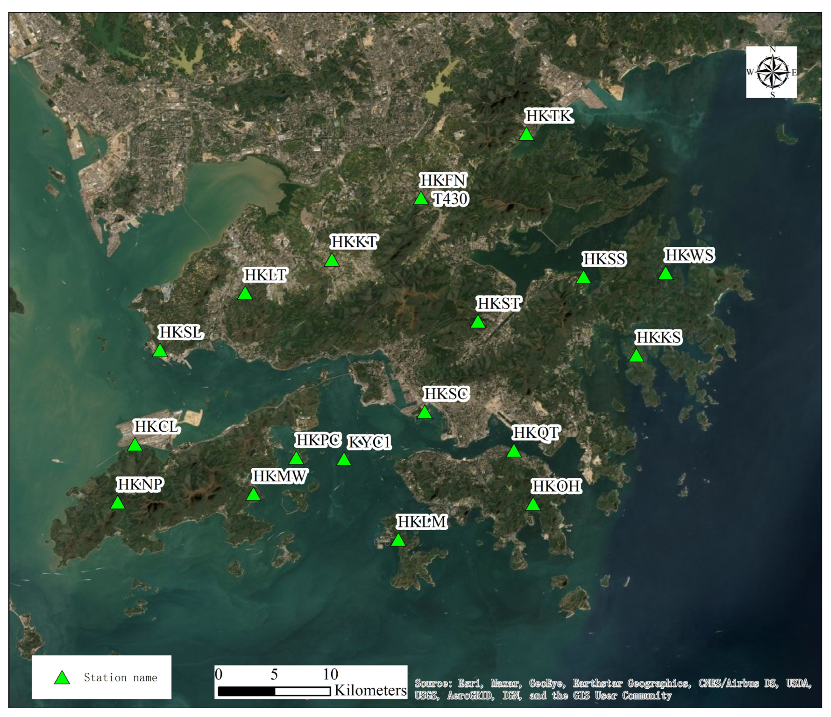
2.2. Hong Kong Satellite Positioning Reference Station Network

To analyze the fitting performance of commonly used ionospheric models in low-latitude regions during a geomagnetic storm, this study selected Hong Kong as the study area. The VTEC value is calculated by the observation data of the Hong Kong Satellite Positioning Reference Station Network (SatRef), and the degree of accuracy loss of different ionospheric models during a strong geomagnetic storm is analyzed. Data source: ftp://ftp.geodetic.gov.hk/ (accessed on 13 October 2021).

The Hong Kong SatRef has a total of 18 continuously operating reference stations, including 9 mountain reference stations and 9 rooftop reference stations. The distance between the reference stations is approximately 10 to 15 km. Figure 1 is the distribution map of the station.

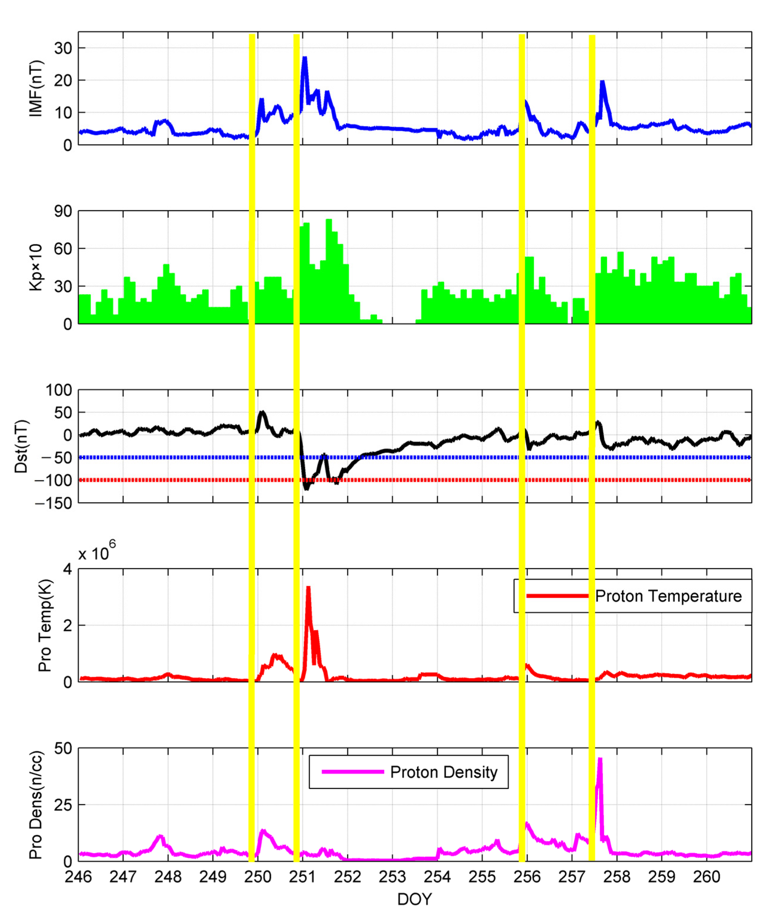
2.3. Space Weather Indices

In this study, some space weather indices were used to analyze the fluctuation characteristics of the magnetic field during the geomagnetic storm, such as: interplanetary magnetic field (IMF) magnitude, Kp, Dst, proton temperature, and proton density. The data came from the NASA’s Space Physics Data Facility (SPDF). SPDF is a project of the Heliophysics Science Division (HSD) at NASA’s Goddard Space Flight Center. SPDF also provides multi-project, cross-disciplinary access to data in order to enable correlative and collaborative research across discipline and mission boundaries with present and past missions.. In this paper, the geomagnetic storm indices (Dst and Kp), magnetic field data (IMF magnitude avg) and plasma data (proton temperature and density) all are 1-h resolution. The Dst index is used as the main indicator for the identification of a geomagnetic storm.

3. Results and Discussion

3.1. Dst Index Fluctuation during Geomagnetic Storm

By analyzing the space weather indices from 3 September 2017 to 17 September 2017, the information of geomagnetic storm start and end times, and storm intensity are described (Figure 2).

In Figure 2, the abscissa is day of year (DOY). It can be seen that there are four SSCs from 246th to 260th. Among them, IMF, Kp, Dst, proton temperature, and proton density all fluctuated significantly after the SSCs of 249th and 250th. However, only IMF, Kp, and proton density fluctuated significantly after the SSCs at 255th and 257th, and the Dst index did not reach the threshold of −50 for a moderate storm. The storm intensity judgment standard is shown in

Table 1. Geomagnetic activity intensity threshold of Dst index.

Geomagnetic Index	Quiet	Moderate Storm	Strong Storm
Dst [nT]	Greater than −50	[−100, −50]	Less than −100

[28].

Usually, the Dst index is used as the basis for judging geomagnetic storms. From Figure 2, it can be found that the Dst index is less than −50 storm threshold only at 251st and 252nd, that is, there were significant geomagnetic storm events in these two days. Dst was at a level greater than 0 before 23:00 on the 249th, indicating that the geomagnetic field was quiet.

In detail, the Dst index dropped sharply at around 0:00 UTC on the 251st, the minimum value was close to −150 nT, and then the Dst index rapidly increased to around −60 nT. At around 12:00 UTC on the 251st, it dropped rapidly again, and the minimum value was close to −125 nT. At about 12:00 UTC on the 252th, it recovered to above −50 nT, and the geomagnetic field entered a relatively quiet state. According to the classification standard of geomagnetic storms in Table 1, this geomagnetic storm is a strong geomagnetic storm event. The geomagnetic field disturbance is significant, and the disturbance time lasts for approximately 48 h. Due to the significant coupling relationship between the geomagnetic field and the ionosphere, geomagnetic storms will have a dramatic impact on the ionosphere [5]. Therefore, this paper selects this storm event to study the activity characteristics of the ionosphere in the low-latitude region during the strong geomagnetic storm and provide a reference for the refinement of the low-latitude ionosphere model. According to the change characteristics of the magnetic field during the geomagnetic storm, it can be divided into three stages, namely, the initial phase, the main phase, and the recovery phase [10]. Combined with the change trend of the Dst index in Figure 2, the corresponding time of the initial phase, main phase, and recovery phase of this geomagnetic storm are shown in

Table 2. Corresponding time of different stages of this geomagnetic storm.

Storm Stage	Period
Initial phase	7 September 2017 UTC 0:00~7 September 2017 UTC 22:00
Main phase	7 September 2017 UTC 23:00~8 September 2017 UTC 3:00
Recovery phase	8 September 2017 UTC 4:00~9 September 2017 UTC 23:00

.

3.2. Time Characteristics of Low-Latitude Ionospheric Disturbance

To explore the change in characteristics of the ionosphere over time during this geomagnetic storm, the time series of the vertical total electron content (VTEC) is analyzed. We select VTEC on two symmetrical grid points in the northern and southern hemispheres of low latitudes as the research object. The positions of grid point 1 and 2 are (22.5° N, 110° E) and (22.5° S, 110° E), respectively. In addition, according to the fluctuation of the Dst index in Figure 2, the geomagnetic activity from 7 to 9 September 2017 was intense, whereas the geomagnetic activity on 6 September 2017 and 10 September 2017 was relatively quiet. Therefore, the ionospheric variation characteristics of these two days are used as a control. The VTEC variation trends of grid points 1 and 2 on 6, 8, and 10 September 2017 were plotted, as shown in Figure 3 and Figure 4, respectively.

Figure 3 shows that the VTEC gradually increases from approximately 12 TECU before (6 September) and after (10 September) the geomagnetic storm and reached a peak at approximately 45 TECU around 7:00 UTC. The time when VTEC starts to decrease is about UTC 9:00; it then decreases sharply from UTC 10:00 to 13:00, and stabilizes at a lower level from UTC 15:00 to 24:00, which VTEC fluctuates slightly at 5–10 TECU. The variation trend of the ionospheric VTEC at grid point 1 in the northern hemisphere before and after the geomagnetic storm is basically the same. It shows an overall trend of first increasing, reaching a peak, and then decreasing; that is, there is a consistency with the diurnal variation, which the VTEC varies with solar altitude. On 8 September, the study area VTEC showed a sharp increase trend at UTC 0:00–6:00, with a peak value of approximately 50 TECU, and entered the VTEC reduction stage from UTC 6:00. Although the variation trend of VTEC in the geomagnetic storm also meets the diurnal variation characteristics, the value of study area VTEC in the period of increasing electron concentration (UTC 0:00–6:00) is significantly higher than those before and after the geomagnetic storm. In addition, in Figure 3, the VTEC on 8 September entered a lowering stage at nearly UTC 6:00, while on 6 and 10 September, the VTEC began to decrease at about UTC 9:00. This observation shows that the time of study area VTEC entering the lowering stage on the disturbed day is earlier than that on the quiet day during the current geomagnetic storm.

In Figure 4, the fluctuation trend of VTEC is at grid point 2 in the southern hemisphere, which is on the same longitude and latitude as grid point 1 in the northern hemisphere. Figure 4 shows that on 6 September (before the storm) the VTEC was in an increasing phase at UTC 0:00–4:00, VTEC increased from approximately 8 TECU to approximately 18 TECU, then began to decline, and stabilized at a lower level from UTC 13:00 to 24:00. On 10 September (after the storm) VTEC also started to increase from approximately 8 TECU, but reached two peaks at UTC 3:00 and UTC 8:00, respectively, and the peak VTECs were approximately 13 TECU and 15 TECU. After that, VTEC stabilized at approximately 3–5 TECU. Compared with the fluctuation trends before and after the geomagnetic storm, that of VTEC in the geomagnetic storm also shows a significant difference. The VTEC increased sharply from about 12 TECU on 8 September (this result is consistent with the findings of Blagoveshchensky et al. [18]) and reached a first peak at UTC 3:00, followed by a rapid decline, started to increase again at UTC 6:00, and reached the second peak at UTC10:00. The VTEC showed a downward trend from UTC 10:00 to UTC 21:00. Two peaks were observed in one day, around 4:00 and 10:00 UTC on September 8th, and the peak value of VTEC is significantly higher than that of 18 TECU before the storm and 15 TECU after the storm, and the maximum peak value exceeds 28 TECU. Form Figure 3 and Figure 4, the VTEC shows an increasing trend during the geomagnetic storm, but the VTEC of grid point 2 in the southern hemisphere is lower than that of grid point 1 in the northern hemisphere. From the VTEC fluctuation on 8 September, the degree of VTEC anomaly (deviation from the statistical level) of grid point 2 is significantly higher than that of grid point 1, indicating that the impact of this geomagnetic storm on the ionosphere in the low latitudes of the southern hemisphere is greater than that of the northern hemisphere.

3.3. Spatial Characteristics of Low-Latitude Ionospheric Disturbance

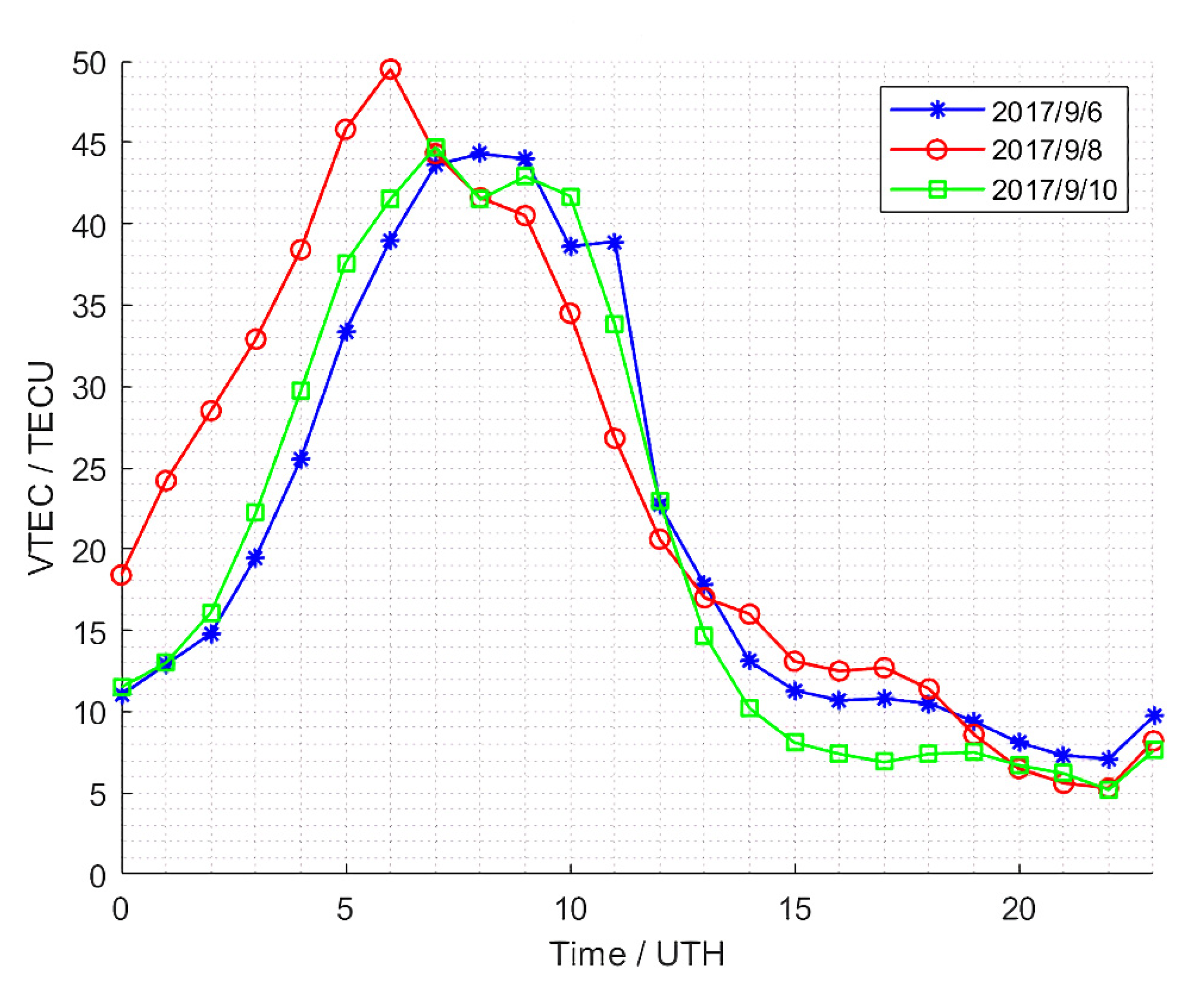
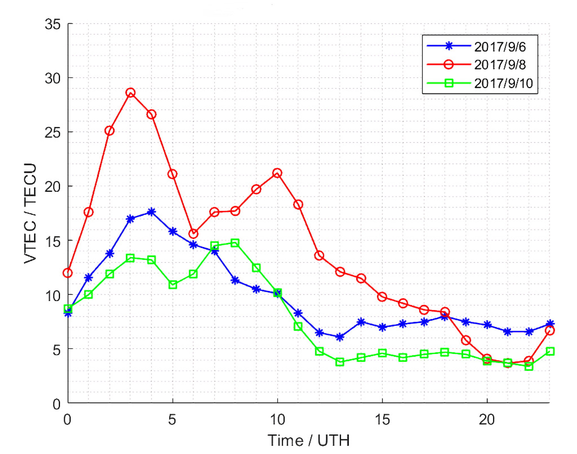
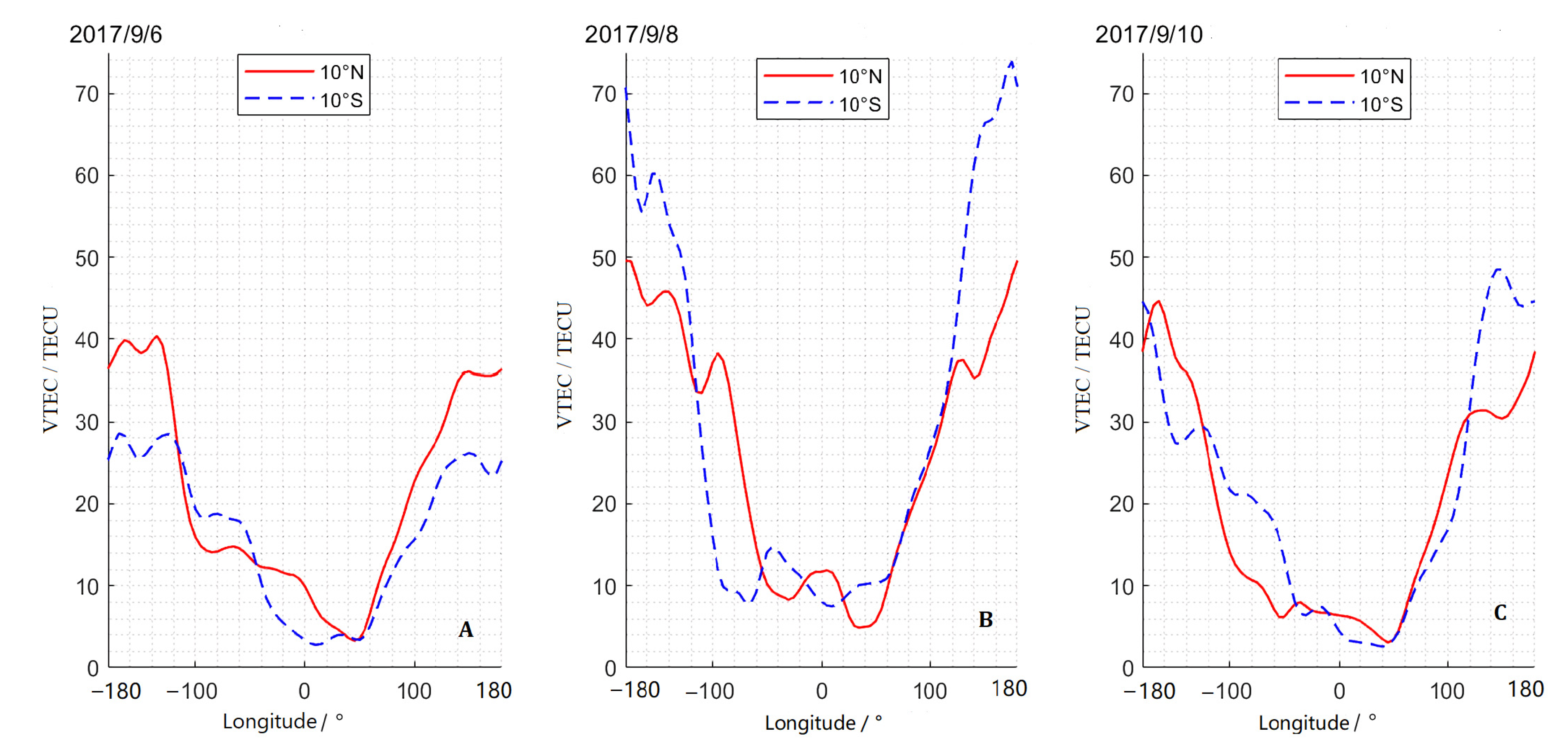
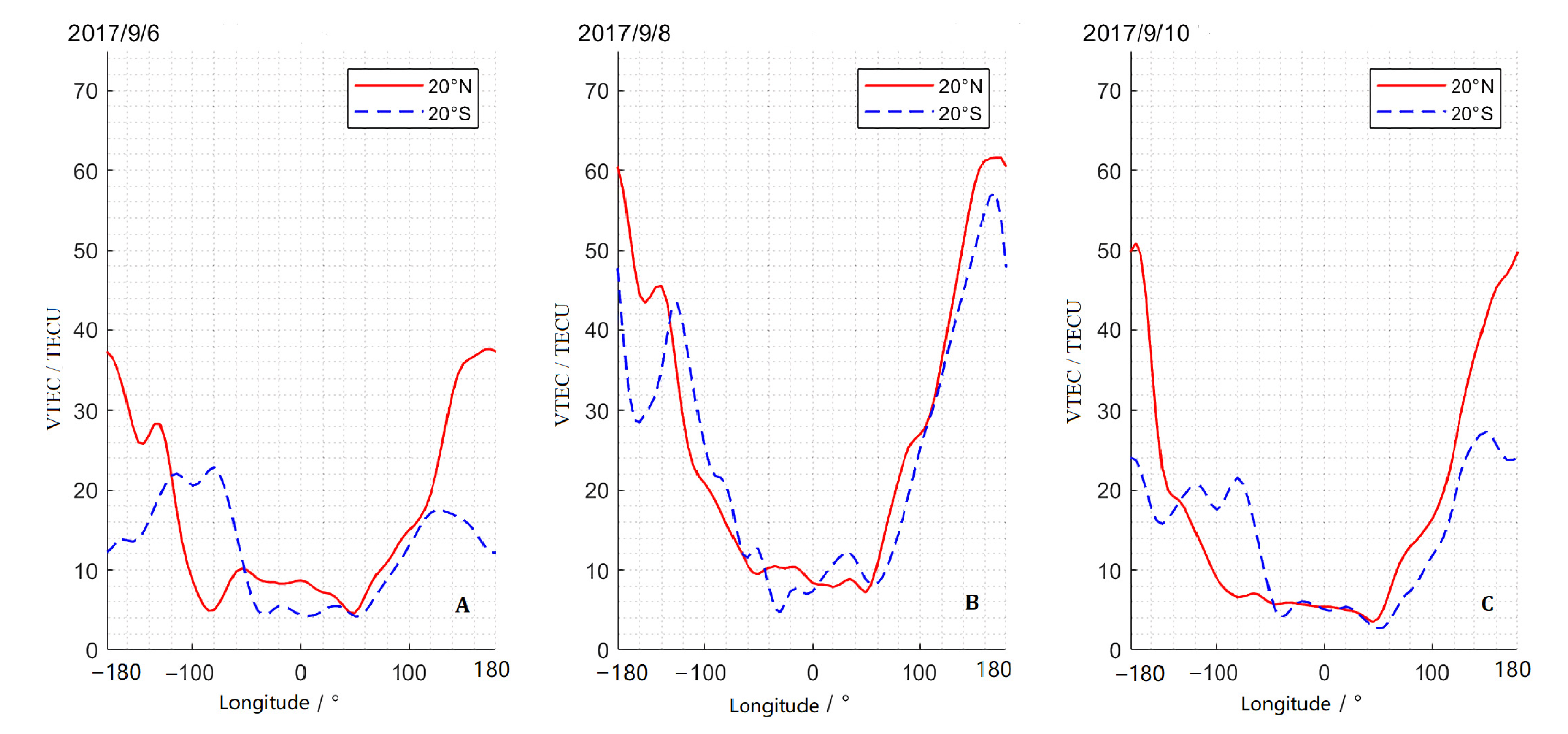
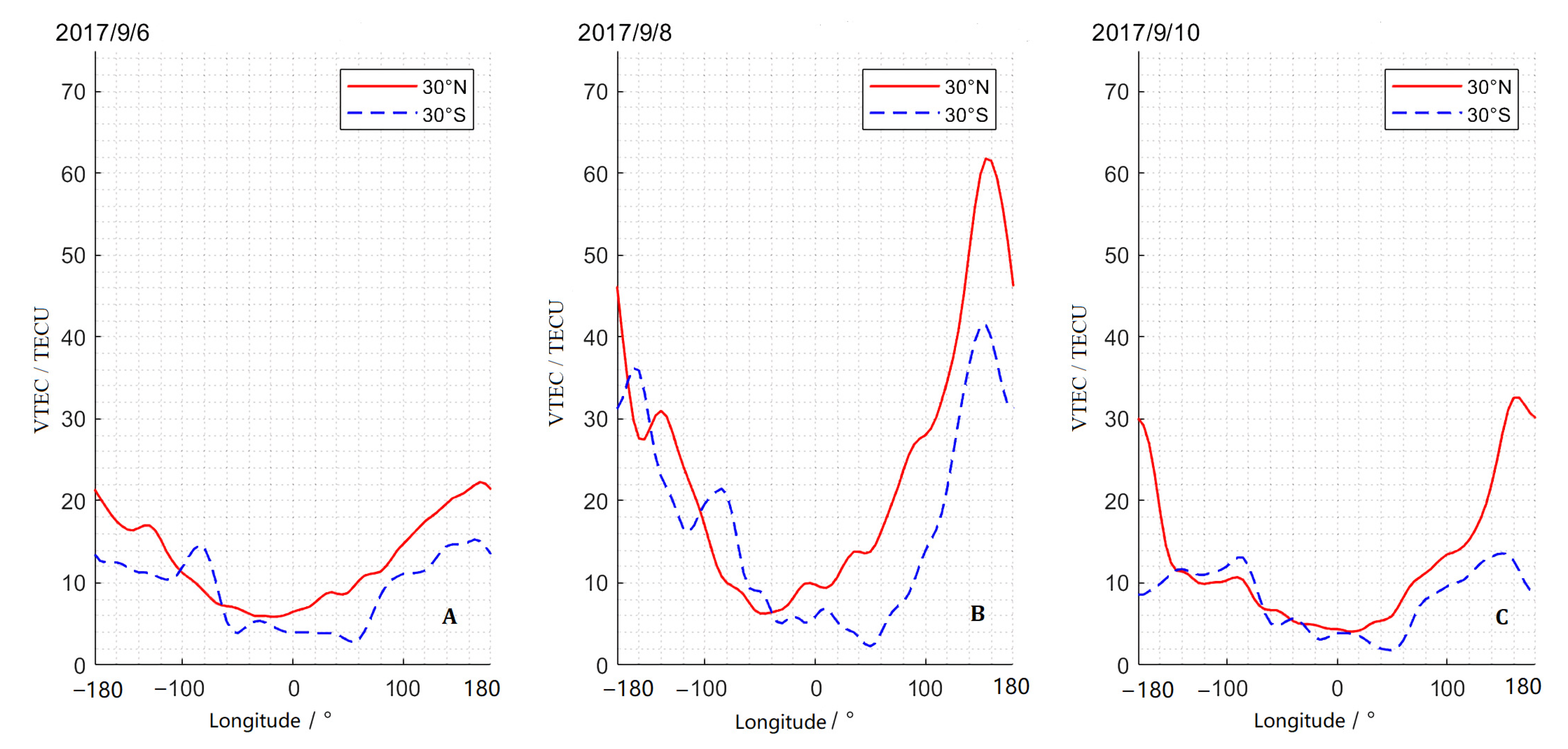
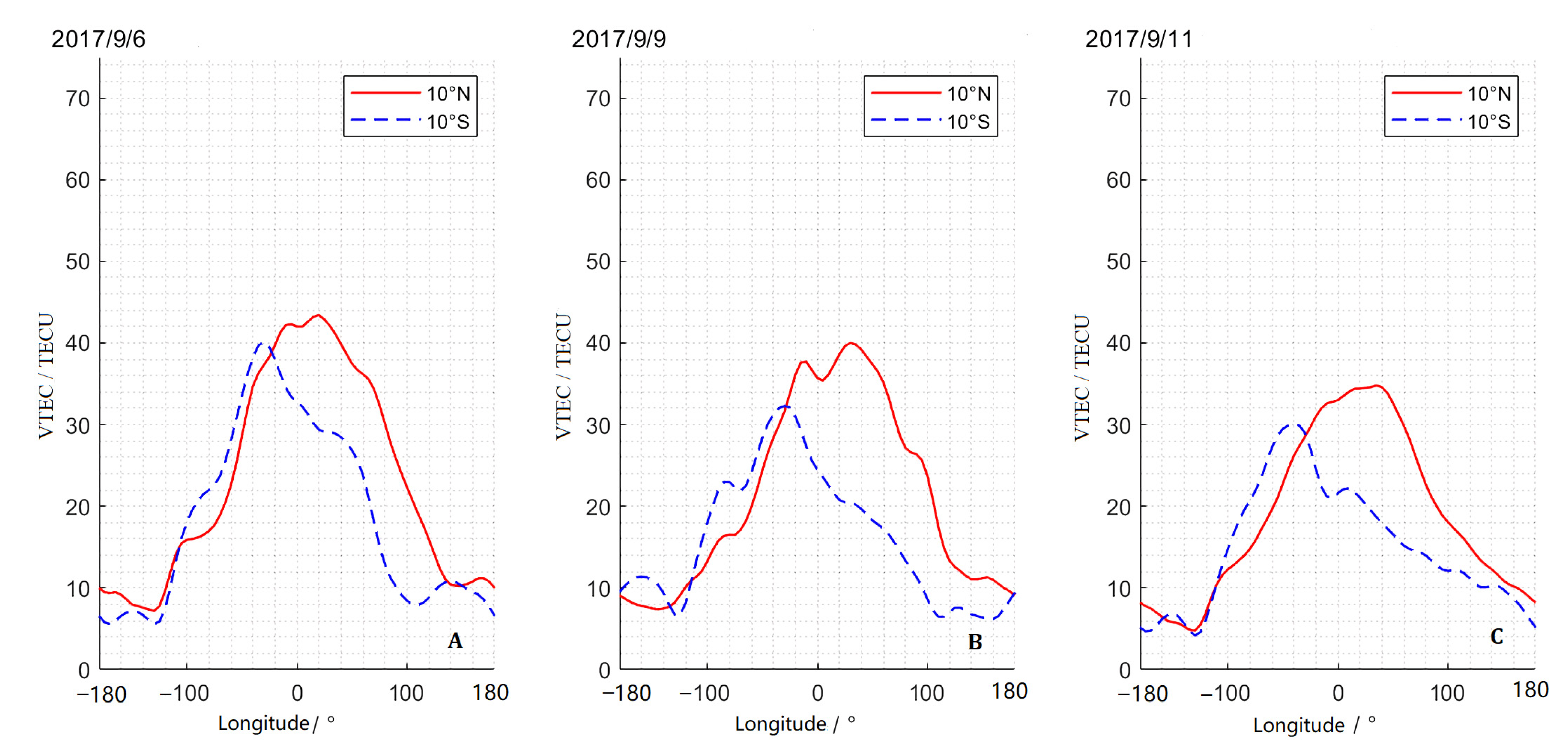
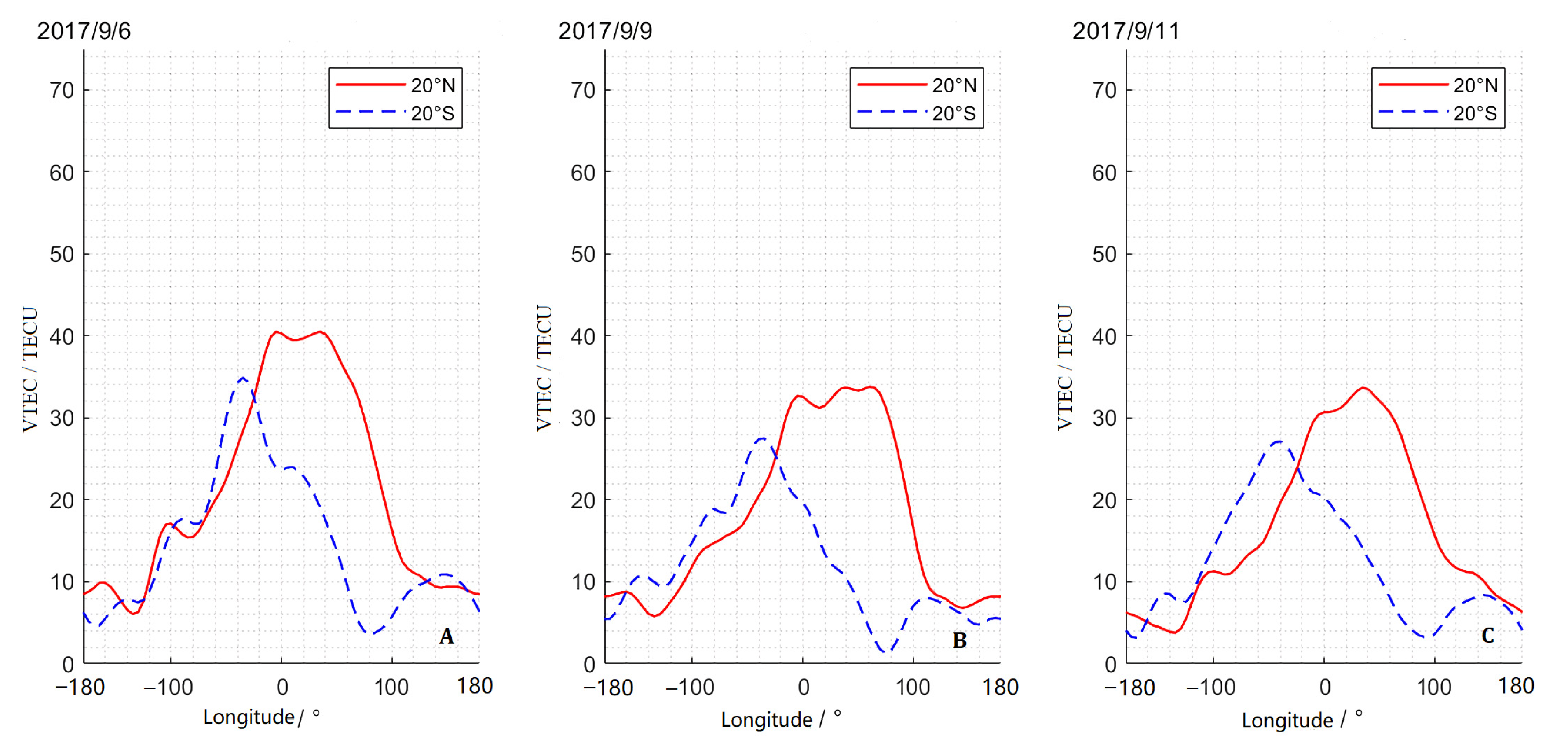
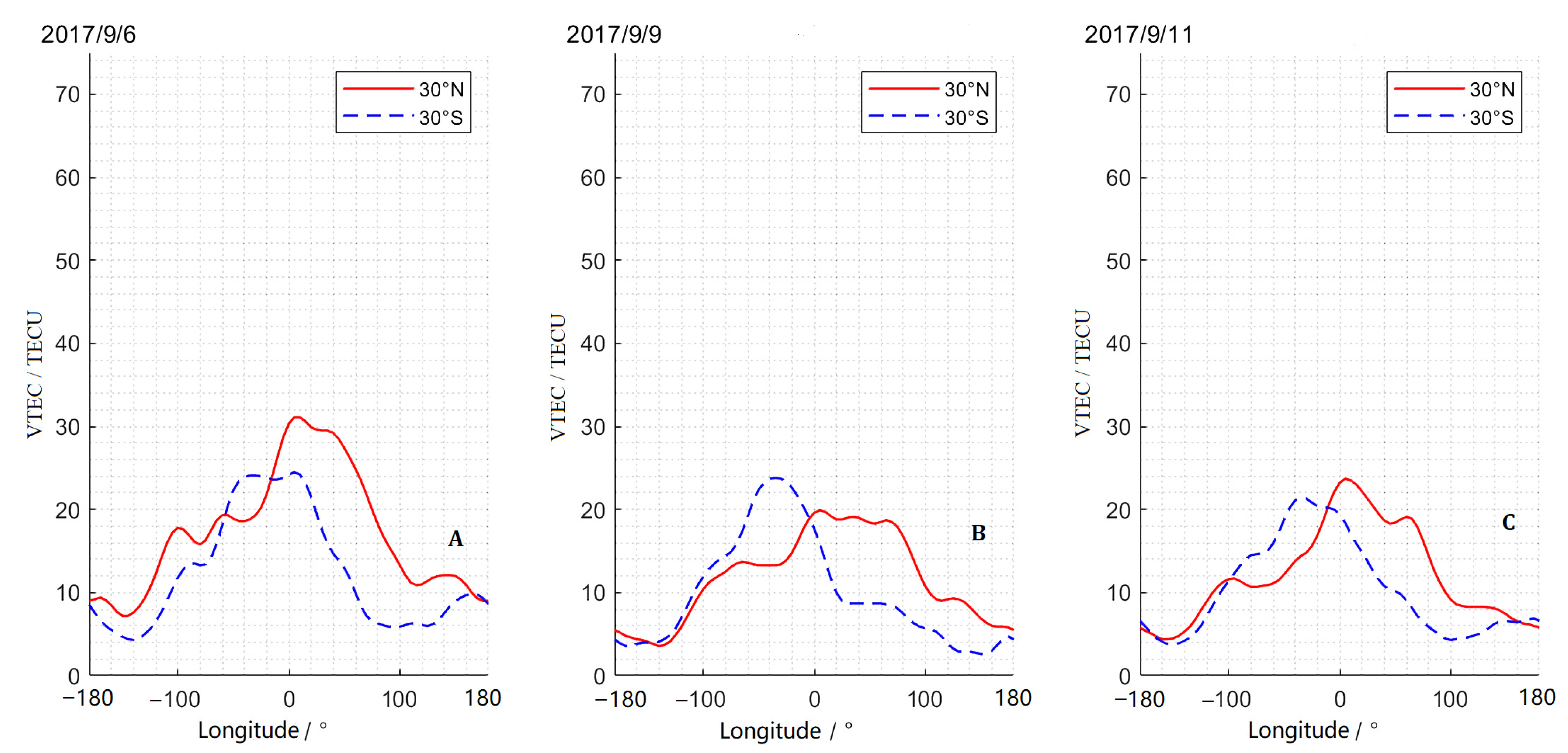
3.3.1. Zonal and Meridional Characteristics of VTEC

To explore the anomalous spatial changes in the ionosphere at low latitudes during geomagnetic storms, this paper analyzes the zonal and meridional changes in the ionosphere. The experiment selected VTEC at low latitudes (30° S—30° N) as the research objects. In each group of experiments, the VTEC before (6 September) and after (10 September) the geomagnetic storm were used as the control group for comparative analysis. In addition, due to the different magnetic field activities in the main phase and the recovery phase of the geomagnetic storm, this paper analyzes the ionospheric activity characteristics of the main phase and the recovery phase, respectively.

1.

Main phase

In the experiment, the VTEC from 180° W to 180° E at six latitudes of 10° N, 10° S, 20° N, 20° S, 30° N, and 30° S was used as the research object. The variation trends of VTEC in the experimental group (8 September) and the control group (6 and 10 September) at UTC 2:00 on the day were plotted, respectively, as shown in Figure 5, Figure 6 and Figure 7.

By analyzing Figure 5, Figure 6 and Figure 7, the variation trends of VTEC at different latitudes in low-latitude regions with longitude all show the characteristics of peak and trough; the VTEC trough is near the zero-degree longitude and the peak is near the 180-degree longitude at UTC 2:00, and the variation trends of VTEC at symmetrical monitoring points in the northern and southern hemispheres are not consistent. However, in the main phase of the geomagnetic storm (the panels B in Figure 5, Figure 6 and Figure 7), the peak value of the wave crest is significantly higher than those before and after the geomagnetic storm. Especially at 10° N/S latitude, the VTEC peak value in the southern hemisphere exceeds 70 TECU, which is approximately 75% higher than the peak value of 40 TECU before and after the geomagnetic storm. This finding indicates a significant increase in the ionospheric VTEC at low latitudes caused by this geomagnetic storm. In addition, by comparing the differences between the northern and southern hemispheres of VTEC peaks before and after the geomagnetic storm (the panels A and C in Figure 5, Figure 6 and Figure 7), we found that the peaks of VTEC at latitudes of 20° and 30° in the northern hemisphere are higher than those in the southern hemisphere. This finding indicates that under geomagnetically quiet conditions, the equatorial anomaly of the ionosphere is not symmetrical in the northern and southern hemispheres. However, during the main phase of the geomagnetic storm, the VTEC increase in the southern hemisphere is higher than that in the northern hemisphere, thereby weakening the difference between the northern and southern hemispheres.

The figures also reflect that at the same latitude, the VTEC valley values of the before, the main phase, and the after of the geomagnetic storm are almost the same, and they all remain around 5 TECU. With the change in the solar hour angle, the VTEC shows a different degree of increasing trend with the change in longitude, thereby changing the VTEC at various longitudes. Figure 6, Figure 7 and Figure 8 show that in the main phase of the geomagnetic storm, the VTEC changes with longitude is significantly more severe than those before and after the magnetic storm. This change trend in the northern hemisphere is significantly more severe than that in the southern hemisphere, which indicates that the longitude change characteristics of the ionosphere are affected by geomagnetic storms and exhibit differences between the northern and southern hemispheres.

2.

Recovery phase

According to the stage division of this geomagnetic storm in Table 1, the recovery phase is mainly on 9 September. Thus, this paper analyzes the meridional and zonal variation characteristics of the low-latitude VTEC on 9 September and uses the VTEC on 6 September and 10 September as the control group. The variation trends of VTEC with longitude on 10° N, 10° S, 20° N, 20° S, 30° N, and 30° S latitudes at UTC 14:00 are plotted as shown in Figure 8, Figure 9 and Figure 10.

Figure 8, Figure 9 and Figure 10 illustrate that the variation in VTEC with longitude at different latitudes in the recovery phase of this geomagnetic storm also shows obvious peak characteristics. However, the VTEC peak value of the recovery phase was not significantly different from those before and after the geomagnetic storm, indicating that the ionospheric activity basically returned to the normal level during the recovery phase of the geomagnetic storm. The VTEC in the southern and northern hemispheres are consistent in regions where VTEC increases with longitude. However, regions where VTEC decreases with longitude show significant differences between the northern and southern hemispheres, that is, the VTEC in the northern hemisphere is significantly higher than those in the southern hemisphere on the same longitude in the region where VTEC decreases with longitude, and the difference is more obvious when the latitude is lower. The reason may be that the interaction between the equatorial current system and the magnetic field causes the deflection of free electrons to the northern hemisphere, resulting in the phenomenon of the VTEC in the northern hemisphere being higher than that in the southern hemisphere, and this phenomenon is not significantly affected by the geomagnetic disturbance of the recovery phase.

In the comparison of the latitude differences of VTEC in Figure 8, Figure 9 and Figure 10, we found that when the latitude is low, the peaks of VTEC at before and after the geomagnetic storm and the recovery phase are higher. The VTEC peak is about 40 TECU at 10° N/S latitude, the VTEC peak is slightly lower than 10° N/S latitude at 20° N/S latitude, and the VTEC peak decreases to about 30 TECU at 30° N/S latitude. In addition, the daily minimum value of VTEC at different latitudes is basically the same, about 5 TECU, that is, the minimum value of VTEC in low latitudes (nighttime VTEC) is weakly affected by latitude and geomagnetic storms.

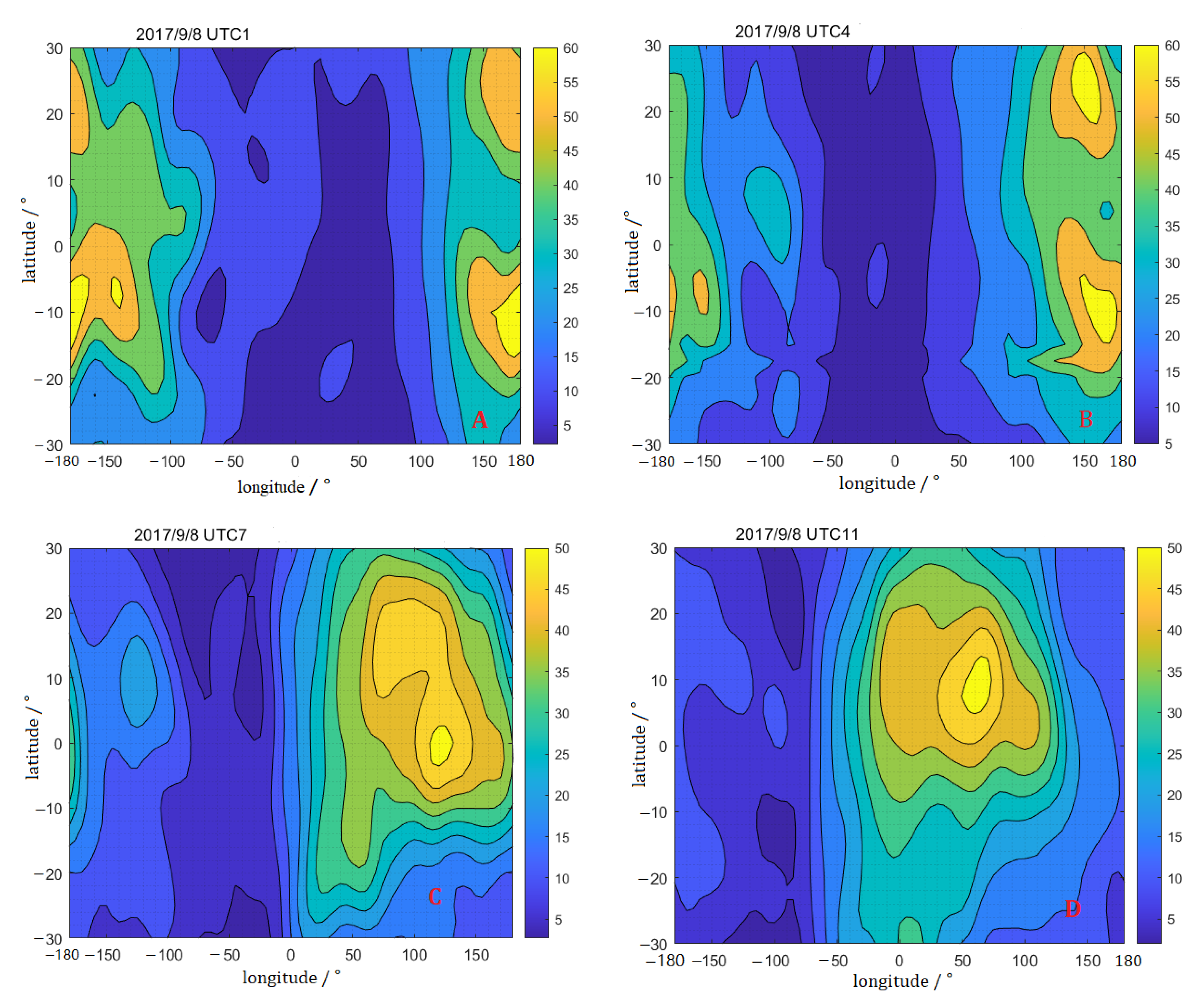
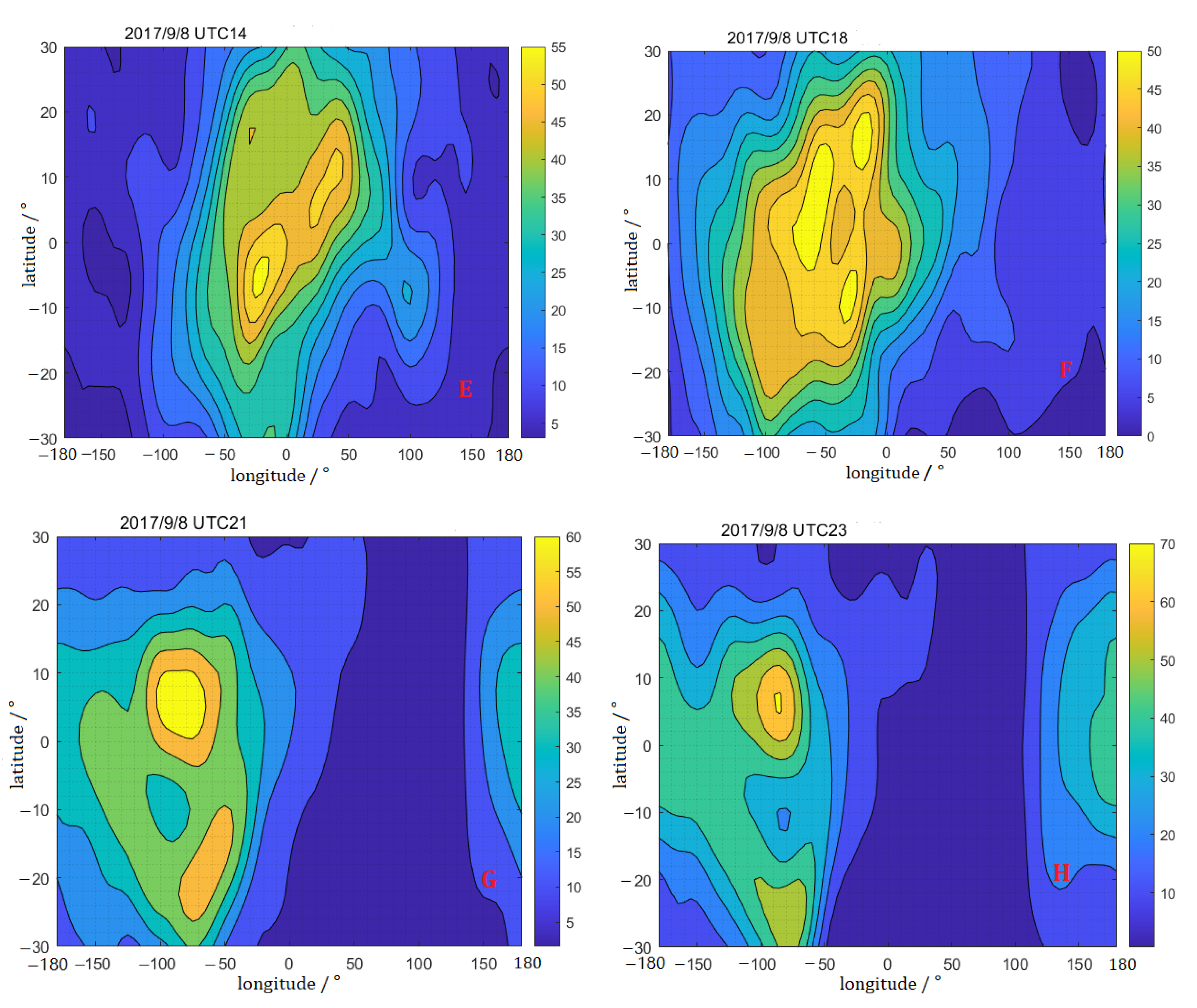
3.3.2. Spatial Distribution Characteristics of VTEC

Another issue to be explored in this paper is the anomalous spatial distribution of low-latitude ionospheric VTEC during geomagnetic storms. Therefore, the ionospheric VTEC value in the region during the geomagnetic storm (30° N~30° S, 180° W~180° E) is selected as the research object. Pseudo-color maps of the VTEC spatial distribution are shown in Figure 11.

The spatial distribution of VTEC in each panel in Figure 11 shows that the peak area of VTEC exhibits a trend of moving from east to west over time. It is closely related to the solar hour angle at different longitudes, indicating that the characteristics of ionospheric activity at low latitudes during magnetic storms are generally consistent with the general pattern of ionospheric activity. In addition, at UTC 1:00, UTC 4:00, UTC 7:00, UTC 14, UTC 21:00, and UTC 23:00, VTEC presents two peak areas in the north and south, showing double peak characteristics, that is, the equatorial “fountain effect” formed under the combined action of the equatorial current system and the geomagnetic field [29,30], which is also consistent with the general characteristics of the ionospheric equatorial anomaly. However, ionospheric anomalies were exhibited at UTC 11:00 and 18:00, with VTEC showing only one peak area at UTC 11:00 and three peak areas at UTC 18:00.

Comparing the Dst index data on 8 September in

Table 3. The Dst index on 8 September 2017.

UTC/H	1	2	3	4	5	6	7	8	9	10	11	12
Dst/nT	−125	−142	−128	−114	−124	−110	−108	−108	−90	−73	−63	−63
UTC/H	13	14	15	16	17	18	19	20	21	22	23	24
Dst/nT	−96	−120	−122	−118	−110	−124	−114	−113	−104	−102	−102	−98

, we found that at UTC 11:00 and UTC 18:00, the Dst index has a minimum value and an extremum value of the day, respectively. Given that the Dst index reflects the strength of the geomagnetic storm, it is inferred that during the geomagnetic storm, the weakening of the magnetic disturbance will weaken the “fountain effect” in the low-latitude ionospheric anomaly, thereby showing the VTEC single-peak characteristic. However, when the magnetic perturbation intensifies, it interferes with the “fountain effect”, hence enabling it to exhibit an anomalous characteristic of multiple peaks. To sum up, from the analysis of the spatial distribution of VTEC, the violent disturbance of the magnetic field during geomagnetic storms will lead to abnormal characteristics of the “fountain effect” in the ionosphere at low latitudes.

3.4. Performance Analysis of Ionospheric Model during Geomagnetic Storm

To explore whether the ionospheric function model was significantly affected during this strong geomagnetic storm, this study separately tested the fitting performance of the spherical harmonics (SH), polynomial model, and ionospheric model based on continuity equation (ICE) models in low latitudes.

3.4.1. Commonly Used Ionospheric Function Models

(1)

SH model

The SH is used to fit the ionospheric VTEC, which is suitable for establishing a global model. The function expression is shown in Formula (1).

$$VTEC={\displaystyle \sum _{n=0}^{n_{\max }}{\displaystyle \sum _{m=0}^n\widetilde{P_{nm}}(\sin {\phi }_p)}}(a_{nm}\cos ms+b_{nm}\sin ms)$$

(1)

where VTEC is the total electron content of the zenith; ${\phi }_p$ is the latitude of the puncture point; s = ${\lambda }_p$ − $s_0$, ${\lambda }_p$, and $s_0$ are the longitude and solar time angles of the puncture point, respectively. a_nm and b_nm are the ionospheric model coefficients to be calculated, P_nm is the normalized Legendre polynomial, and n and m are the model order [31,32,33,34]. The SH can be used not only for global ionospheric modeling but also for regional ionospheric modeling. For example, low-order SH can be used to model the ionosphere in a small area.

(2)

Polynomial model

The polynomial model regards the VTEC of the ionosphere as a function, and the difference in solar time angle and latitude, and the model expression is shown in (2),

$$VTEC={\displaystyle \sum _{i=0}^m{\displaystyle \sum _{j=0}^n{a}_{ij}{({\phi }_p-{\phi }_0)}^i{(s-s_0)}^j}},$$

(2)

where ${\phi }_0$ is the geographic latitude of the central point of the study area, $s_0$is the solar hour angle of the station position $({\phi }_0, {\lambda }_0)$ at time $t_0,$ $s-s_0=\left({\lambda }_p-{\lambda }_0\right)+\left(t_i-t_0\right)$. $({\lambda }_p, {\phi }_p)$ is the longitude and latitude of the puncture point, $t_i$ is the observation time, $a_{ij}$ is the model coefficient to be estimated, and m and n are the highest order [35,36,37]. When the number of observations is more than the parameters of the equation, the least square method is used to obtain the optimum values. The polynomial model is a common model for region modeling, but suffers from “edge effects” when modeling a larger region.

(3)

ICE model

Taking into account the photochemical reactions and transportation in the ionosphere, a new ionospheric model is established by Li et al., named ICE model [8]. The model expression is shown in Formula (3).

$$\{\begin{array}{l}f({\phi }_0,\lambda )=\frac{-K_3+{\{K_3^2-4K_2[K_1{I}^{\prime }(\sin {\phi }_0\sin \delta +\cos {\phi }_0\cos \delta \cos \lambda )-K_4]\}}^{\frac{1}{2}}}{2K_2},(-90<\lambda <90)\\ f({\phi }_0,\lambda )=\frac{-K_3}{2K_2}+\frac{1}{2K_2}{(K_3^2+4K_2{K}_4)}^{\frac{1}{2}}=K_0,(\lambda \le -90,90\le \lambda )\\ \lambda =\frac{2\pi \left(\mathrm{t}-14\right)}{24}\end{array}$$

(3)

where the δ is the declination of the sun, ${\phi }_0$ represents the geographic latitude of the observation location, t is the local time, and $\lambda$ is the hour angle (the hour angle takes 14:00 local time as 0°, that is, the sun is at the local time at 14:00 when it rises to the highest position in the day), I^′ is the solar radiation flux. The ICE model regards the total electron content in a small area of the night hemisphere as a constant $K_0$. The $K_0$, $K_1$, $K_2$, $K_3$, and $K_4$ are parameters related to the physical properties of the ionosphere. Similarly, parameter estimation equations can be established by GNSS observations, model coefficients are estimated by the least square method, and the ICE model expression used to calculate the local TEC can be obtained.

3.4.2. Principle of GNSS Ionospheric VTEC Inversion

In this study, GNSS dual-frequency observations are used as experimental data, and the carrier phase smoothed pseudorange method is used to calculate the slant TEC (STEC) in the line of sight (LOS). Then, the mapping function is used to calculate the VTEC of the puncture point; the main principle is shown in the Formulas (4)–(7).

Firstly, geometry-free pseudorange P4 is constructed by inter-frequency differencing by GNSS multi-frequency observations as Formula (4).

$${(P_j^i)}_4={(P_j^i)}_1-{(P_j^i)}_2=40.309\times (\frac{1}{f_1^2}-\frac{1}{f_2^2})\times STEC+DC{B}^i+DC{B}_j+{\xi }_P$$

(4)

where $f_1$ and $f_2$ are GNSS signal frequencies, $DC{B}^i$ and $DC{B}_j$ are the satellite and receiver differential code bias, respectively.${\zeta }_P$ is the residual, i and j are the satellite and receiver numbers, respectively.

Secondly, the phase-smoothed pseudo-range P₄, sm is obtained by smoothing the pseudo-range observation value by the GNSS phase observation value, and its function expression is as Formula (4).

$$\{\begin{array}{l}{P}_{4,sm}(t)={\varpi }_t{P}_4(t)+(1+{\varpi }_t)P_{4,prd}(t),(t>1)\\ P_{4,prd}(t)=P_{4,sm}(t-1)+[L_4(t)-L_4(t-1)],(t>1)\end{array}$$

(5)

where t represents the number of epochs, ω is the weighting factor related to epoch t, P₄ and L₄ are, respectively, the pseudorange and phase observations without geometric influence constructed by inter-frequency difference in GNSS multi-frequency observations. From Formulas (4) and (5), the expression of phase-smoothed pseudorange observations can be obtained, such as Formula (6).

$$P_{4,sm}=40.3\times (\frac{1}{f_1^2}-\frac{1}{f_2^2})\times STEC+DC{B}^i+DC{B}_j$$

(6)

Finally, under the assumption of the single layer model (SLM), the mapping function is used to convert the STEC to the VTEC at the puncture point, as shown in Equation (7).

$$\{\begin{array}{l}VTEC=M(Z^{\prime })\times STEC\\ M(Z^{\prime })=\cos [\arcsin (\frac{R_e}{R_e+H}\cos E)]\end{array}$$

(7)

where M is the mapping function, $R_e$ is the average radius of the earth, $Z^{\prime }$ is the zenith distance of the puncture point, and E is the altitude angle of the satellite. The H is the effective height of the SLM, generally 300–500 km.

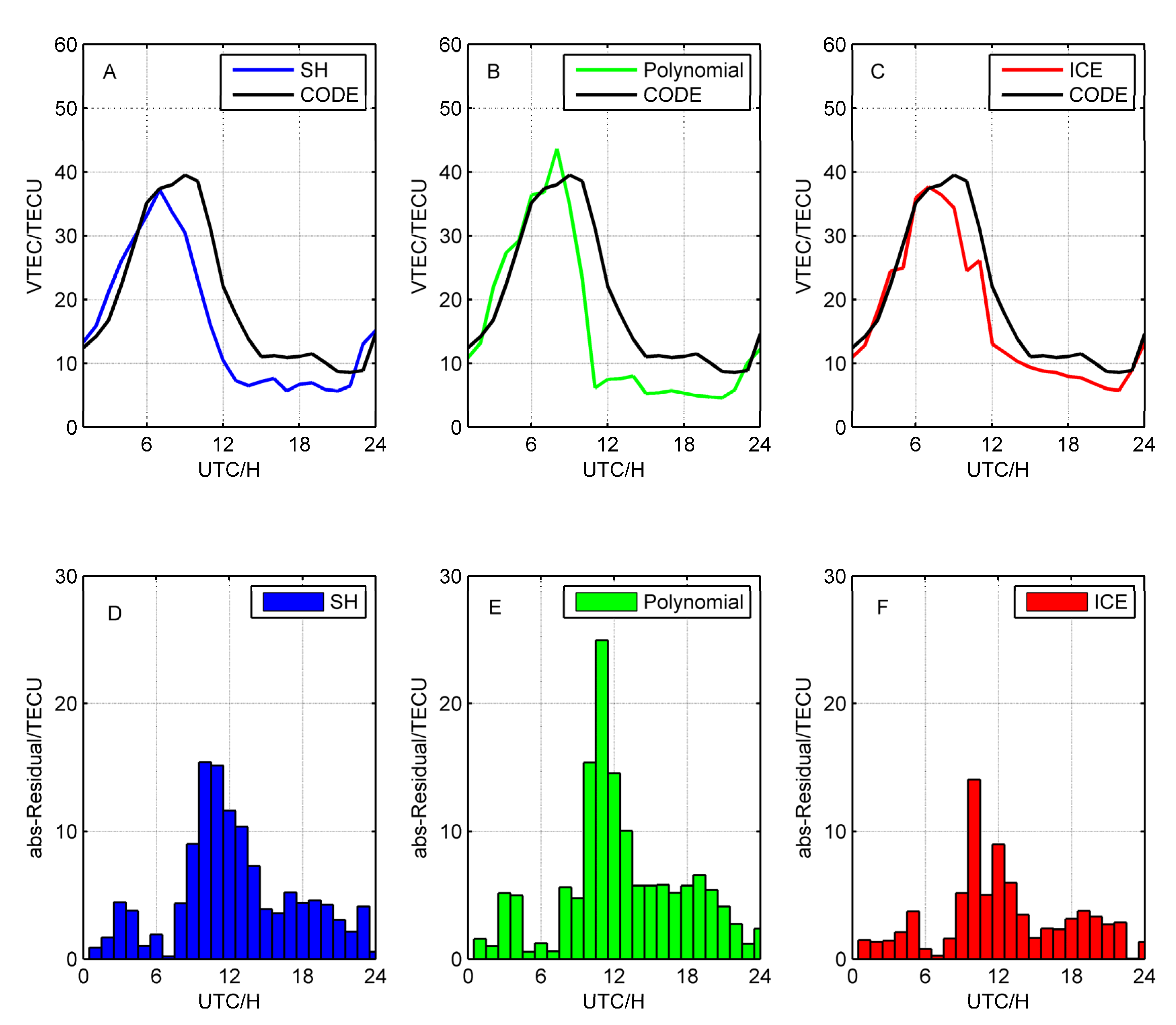
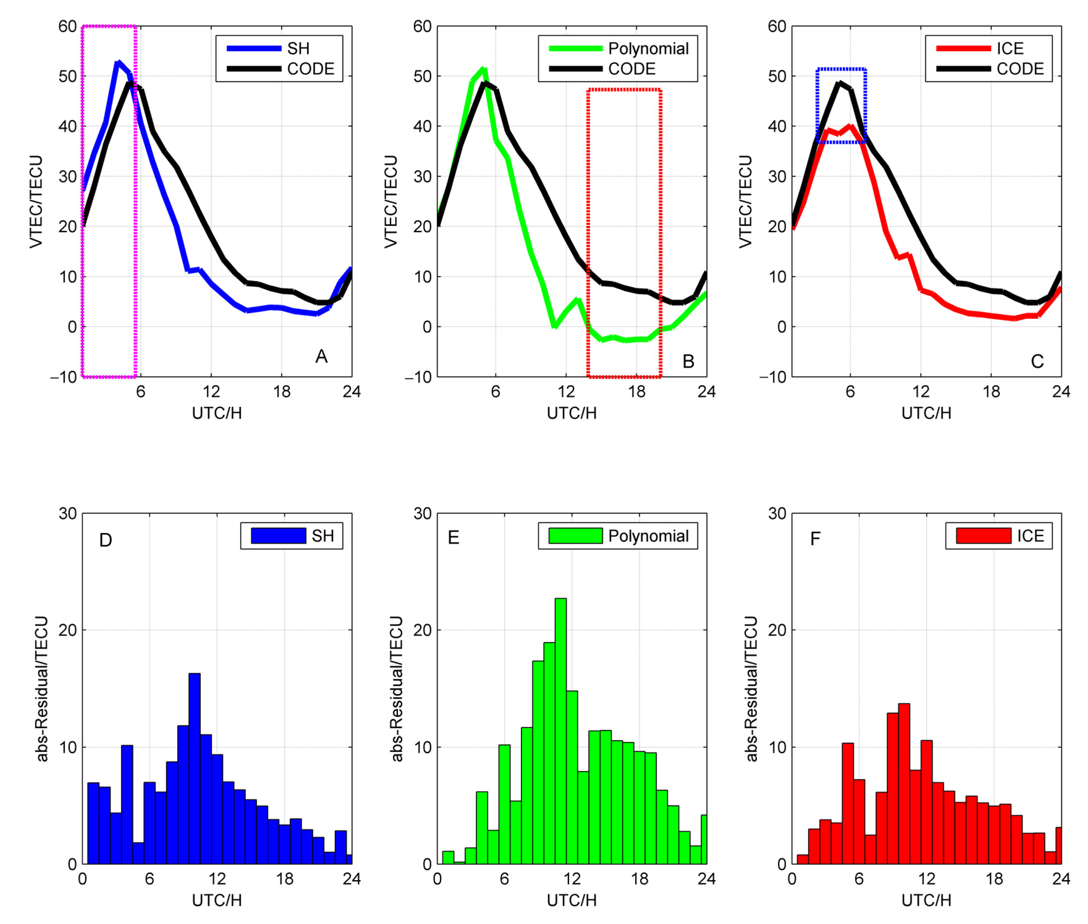
3.4.3. Performance Analysis of Commonly Used Ionospheric Models

Figure 3 shows that 6 September 2017 is a geomagnetic quiet day, and 9 September 2017 is a geomagnetic disturbance day. Therefore, the observation data of Hong Kong SatRef on 6 September and 9 September is used to calculate the daily time series of VTEC at the observation point (22°26′00″ N, 114°12′00″ E), and the fitting performance of the SH, polynomial, and ICE models is analyzed in the Hong Kong region. Since the GIM products released by the IGS Ionospheric Analysis Center have high accuracy and reliability [24,38], the CODE VTEC product is used as a reference value to analyze the performance of three ionospheric models on the geomagnetic quiet day and disturbed day, and the results are shown in Figure 12 and Figure 13.

Figure 12 and Figure 13 show the VTEC time series and absolute residuals for the quiet and disturbance day, respectively. Figure 12 shows that the three models are in good agreement with the reference values from 0:00 to 6:00 UTC, but all exhibit negative systematic biases from 7:00 to 22:00 UTC. It shows that the three ionospheric models have higher fitting accuracy when the VTEC increases on the quiet day, but the model accuracy decreases in the stage of decreasing VTEC.

In Figure 13, the time series of VTEC show that the negative systematic bias of the three models still exists in the stage of decreasing VTEC on the disturbance day. Simultaneously, the SH model shows a positive systematic bias during the VTEC increase phase (UTC 0:00–6:00), which is marked by the pink dotted rectangle. The polynomial model has a negative value of VTEC (red dotted rectangle area) at UTC 14:00–20:00, which is inconsistent with the actual situation. The abnormal feature of the ICE model is that the ionospheric VTEC peak is significantly lower than the reference values by approximately 10 TECU, which is marked by blue dotted rectangle area. To sum up, it shows that the geomagnetic disturbance caused serious distortion in three ionospheric models.

To quantify the degradation level of the model accuracy during a geomagnetic storm, this study counts the absolute residual mean and RMSE, which are calculated by SH, polynomial, and ICE models on the quiet and the disturbed day in Figure 12 and Figure 13.

More ionospheric information can be obtained by using higher temporal resolution when calculating TEC [39,40]. Therefore, the performance of the above three ionospheric models were tested at the temporal resolution of 15 min, 30 min, and 1 h, respectively. Compared with the quiet day, the change percentages on the disturbance day were calculated of the two, and the results are shown in

Table 4. Accuracy statistics of three ionospheric models on the disturbance and quiet day (unit: TECU).

		Mean			RMSE
		SH	Pliynomial	ICE	SH	Pliynomial	ICE
15 min	Quiet	2.781	5.111	3.599	1.788	2.916	2.636
	Disturbance	3.096	4.646	5.523	3.096	4.646	5.523
	Percentage	11.33%	−9.09%	53.45%	73.15%	59.33%	109.52%
30 min	Quiet	3.364	4.349	3.398	3.001	3.823	3.224
	Disturbance	4.123	6.147	5.766	3.459	5.475	4.917
	Percentage	22.56%	41.34%	69.69%	15.26%	43.21%	52.51%
1 h	Quiet	5.121	5.875	3.283	6.612	8.027	4.428
	Disturbance	6.043	8.471	5.654	7.083	10.264	6.579
	Percentage	18.00%	44.19%	72.22%	7.12%	27.87%	48.58%

. Among them, the calculation methods of mean and RMSE are shown in Formulas (8) and (9), respectively.

$$Mean=\frac{{{\displaystyle \sum }}_{i=1}^n\left|VTE{C}_M^i-VTE{C}_{CODE}^i\right|}{n},$$

(8)

$$RMSE=\sqrt{\frac{{{\displaystyle \sum }}_{i=1}^n{\left(VTE{C}_M^i-VTE{C}_{CODE}^i\right)}^2}{n},}$$

(9)

where $VTE{C}_M^i$ is fitting VTEC with different ionospheric models, $VTE{C}_{CODE}^i$ is the VTEC product provided by CODE, the i is the period number, n is equal to 96, 48, or 24 when the temporal resolution is 15 min, 30 min, or 1 h, respectively.

In Table 4, “Mean” is the daily mean value of the absolute residuals, which the ionospheric models compared to the CODE VTEC, “RMSE” stands for root mean square error, “Percentage” shows the change percentage of each indicator on the disturbed day relative to that of the quiet day. From Table 4, it can be seen that on the disturbance day, the residual average values and RMSE of the three ionospheric models are significantly higher than those on the quiet day, and there are similar trends in different temporal resolutions. In addition, it can be found that there is only one negative of the change percentage, which is the “Mean” of the polynomial model at 15 min resolution, and all others are positive. The maximum value of “percentage” is 109.52%, the minimum non-negative value is 7.12%, and the average value is 42.24%. The above table shows that the geomagnetic disturbance leads to a significant decrease in the ionospheric model accuracy.

In addition, it can be seen from Table 4 that the “Percentage” of the ICE model is the largest, followed by the polynomial model, and the SH model has the smallest. This indicates that among the three ionospheric models analyzed in this study, the ICE model is the most affected, followed by the polynomial model, and the SH model is least affected by geomagnetic storms.

4. Conclusions

The disturbance of the ionosphere by space weather, such as solar storms and geomagnetic disturbances, will lead to a significant decrease in the accuracy of the GNSS ionospheric models and will have a negative impact on navigation and positioning services. To determine the disturbance characteristics of the ionosphere at low latitudes during a geomagnetic storm and its impact on the performance of the ionosphere model, this study conducted an in-depth analysis of the anomalous activities of the ionosphere at low latitudes during a strong storm in September 2017 and reached the following conclusions:

• This geomagnetic storm caused the VTEC peak value at low latitudes to be significantly higher than that of the quiet day, and the VTEC peak value increased by approximately 75%. During this geomagnetic storm, the increase in VTEC is mainly concentrated in the rising phase of the VTEC in the northern hemisphere, while it leads to the abnormal phenomenon of two peaks of VTEC in one day in the southern hemisphere.
• In the low-latitude regions where VTEC decreases with the change in longitude, the total VTEC in the northern hemisphere is significantly higher than that in the southern hemisphere on the same longitude, and the lower the latitude is, the more obvious the difference will be. This phenomenon is not significantly affected by the geomagnetic disturbance of the recovery phase.
• The daily minimum value of VTEC at different latitudes was basically the same during this geomagnetic storm, at about 5 TECU, indicating that the minimum value of the ionospheric VTEC (nighttime VTEC) in low latitudes was weakly affected by latitude and geomagnetic storms.
• It is inferred that during the geomagnetic storm, the weakening of the magnetic disturbance will weaken the “fountain effect” in the low-latitude ionospheric anomaly, thereby showing the VTEC single-peak characteristic. However, when the magnetic perturbation intensifies, it interferes with the “fountain effect”, hence enabling it to exhibit an anomalous characteristic of multiple peaks.
• When the model temporal resolution is 1 h, this geomagnetic storm event causes the accuracy of SH, polynomial, and ICE models to decrease by 7.12%, 27.87% and 48.56%, respectively, and cause serious distortion, which are negative VTEC values fitted by the polynomial model.

References

1. Krypiak-Gregorczyk, A.; Wielgosz, P.; Jarmo Owski, W. A new TEC interpolation method based on the least squares collocation for high accuracy regional ionospheric maps. Meas. Sci. Technol. 2017, 28, 045801. [Google Scholar] [CrossRef]
2. Tsurutani, B.; Mannucci, A.; Iijima, B. Global dayside Ionospheric uplift and enhancement associated with interplanetary electric fields. J. Geophys. Res. 2004, 109, A08302. [Google Scholar] [CrossRef]
3. Elias, A.G.; Barbas, B.F.; Zossi, B.S.; Medina, F.D.; Fagre, M.; Venchiarutti, J.V. Review of Long-Term Trends in the Equatorial Ionosphere Due the Geomagnetic Field Secular Variations and Its Relevance to Space Weather. Atmosphere 2022, 13, 40. [Google Scholar] [CrossRef]
4. Zhao, J.; Zhou, C. On the optimal height of ionospheric shell for single-site TEC estimation. GPS Solut. 2018, 22, 48. [Google Scholar] [CrossRef]
5. Liu, Y.; Fu, L.; Wang, J.; Zhang, C. Studying Ionosphere Responses to a Geomagnetic Storm in June 2015 with Multi-Constellation Observations. Remote Sens. 2018, 10, 666. [Google Scholar] [CrossRef]
6. Lean, J.L.; Meier, R.R.; Picone, J.M.; Emmert, J.T. Ionospheric total electron content: Global and hemispheric climatology. J. Geophys. Res. Space Phys. 2011, 116, A10318. [Google Scholar]
7. Li, J.; Huang, D.; Zhao, Y.; Hassan, A. Receiver DCB analysis and calibration in geomagnetic storm-time using IGS products. Surv. Rev. 2019, 53, 122–135. [Google Scholar] [CrossRef]
8. Li, J.; Huang, D.; Wang, Y.; Zhao, Y. A New Model for Total Electron Content based on Ionospheric Continuity Equation. Adv. Space Res. 2020, 66, 911–931. [Google Scholar] [CrossRef]
9. Schmölter, E.; Jens, B. Predicting the Effects of Solar Storms on the Ionosphere Based on a Comparison of Real-Time Solar Wind Data with the Best-Fitting Historical Storm Event. Atmosphere 2021, 12, 1684. [Google Scholar] [CrossRef]
10. Meza, A.; Van Zele, M.A.; Brunini, C.; Cabassi, I.R. Vertical total electron content and geomagnetic perturbations at mid- and sub-auroral southern latitudes during geomagnetic storms. J. Atmos. Sol.-Terr. Phys. 2005, 67, 315–323. [Google Scholar] [CrossRef]
11. Blagoveshchensky, D.V.; Pirog, O.M.; Polekh, N.M.; Christyakova, L.V. Mid-latitude effects of the May 15, 1997 magnetic storm. J. Atmos. Sol.-Terr. Phys. 2003, 65, 203–210. [Google Scholar] [CrossRef]
12. Bagiya, M.S.; Joshi, H.P.; Iyer, K.N.; Aggarwal, M.; Ravindran, S.; Pathan, B.M. TEC variations during low solar activity period (2005–2007) near the Equatorial Ionospheric Anomaly Crest region in India. Ann. Geophys. 2009, 27, 1047–1057. [Google Scholar] [CrossRef]
13. Abdu, M.; Maruyama, T.; Batista, I.S.; Saito, S.; Nakamura, M. Ionospheric responses to the October 2003 superstorm: Longitude/local time effects over equatorial low and middle latitudes. J. Geophys. Res. 2007, 112, A10306. [Google Scholar] [CrossRef]
14. Jiangang, Y.; Wang, L.; Shengnan, L. Response analysis of the global ionosphere to the strong geomagnetic storm on March 17, 2015. J. Surv. Mapp. Sci. Technol. 2019, 36, 559–564. [Google Scholar]
15. Yamauchi, M.; Sergienko, T.; Enell, C.-F.; Schillings, A.; Slapak, R.; Johnsen, M.G.; Tjulin, A.; Nilsson, H. Ionospheric response observed by EISCAT during the September 6–8, 2017, space weather event: Overview. Space Weather 2018, 16, 1437–1450. [Google Scholar] [CrossRef]
16. Jin, H.; Zou, S.; Chen, G.; Yan, C.; Zhang, S.; Yang, G. Formation and evolution of low-latitude F region field-aligned irregularities during the 7–8 September 2017 storm: Hainan coherent scatter phased array radar (HCOPAR) and Hainan digisonde observations. Space Weather 2018, 16, 648–659. [Google Scholar] [CrossRef]
17. Scolini, C.; Chan, E.; Temmer, M.; Kilpua, E.K.J.; Dissauer, K.; Veronig, A.M.; Palmerio, E.; Pomoell, J.; DumboviÄ, M.; Guo, J.; et al. CME CME Interactions as Sources of CME Geoeffectiveness: The Formation of the Complex Ejecta and Intense Geomagnetic Storm in 2017 Early September. Astrophys. J. Suppl. Ser. 2020, 247, 21–48. [Google Scholar] [CrossRef]
18. Blagoveshchensky, D.V.; Sergeeva, M.A. Impact of geomagnetic storm of September 7–8, 2017 on ionosphere and HF propagation: A multi-instrument study. Adv. Space Res. 2019, 63, 239–256. [Google Scholar] [CrossRef]
19. Imtiaz, N.; Younas, W.; Khan, M. Response of the low- to mid-latitude ionosphere to the geomagnetic storm of September 2017. Ann. Geophys. 2020, 38, 359–372. [Google Scholar] [CrossRef]
20. Jin, S.; Jin, R.; Kutoglu, H. Positive and negative ionospheric responses to the March 2015 geomagnetic storm from BDS observations. J. Geod. 2017, 91, 613–626. [Google Scholar] [CrossRef]
21. Xiaoman, Q.; Fuyang, K. Influence of typhoon on ionospheric TEC under different terrain conditions. J. Surv. Mapp. Sci. Technol. 2019, 36, 353–363. [Google Scholar]
22. Mukhtarov, P.; Pancheva, D.; Andonov, B.; Pashova, L. Global tec maps based on gnss data: 1. empirical background tec model. J. Geophys. Res. Space Phys. 2013, 118, 4594–4608. [Google Scholar] [CrossRef]
23. Elmunim, N.A.; Mardina, A.; Siti, A.B. Evaluating the Performance of IRI-2016 Using GPS-TEC Measurements over the Equatorial Region. Atmosphere 2021, 12, 1243. [Google Scholar] [CrossRef]
24. Feltens, J. The International GPS Service (IGS) Ionosphere Working Group. Adv. Space Res. 2003, 31, 635–644. [Google Scholar] [CrossRef]
25. Schaer, S. Mapping and Predicting the Earth’s Ionosphere Using the Global Positioning System. Ph.D. Thesis, Astronomical Institute, University of Berne, Berne, Switzerland, 1999. [Google Scholar]
26. Feltens, J. Development of a new three-dimensional mathematical ionosphere model at European Space Agency/European Space Operations Centre. Space Weather 2007, 5, 1–17. [Google Scholar] [CrossRef]
27. Xinhui, Z.; Longlong, Z.; Ren, W. Ground-based GNSS ionospheric tomography method and application. J. Surv. Mapp. Sci. Technol. 2019, 36, 551–557. [Google Scholar]
28. Palacios, J.; Guerrero, A.; Cid, C.; Saiz, E.; Cerrato, Y. Defining scale thresholds for geomagnetic storms through statistics. Nat. Hazards Earth Syst. Sci. Discuss. 2017, 1–19. [Google Scholar] [CrossRef]
29. Nianlu, X.; Cunchen, T.; Xingjian, L. An Introduction to Ionospheric Physics; Wuhan University Press: Wuhan, China, 1999. [Google Scholar]
30. Tongxing, F.; Wu, Z.; Hu, P.; Zhang, X. Fluctuation of Lower Ionosphere Associated with Energetic Electron Precipitations during a Substorm. Atmosphere 2021, 12, 573. [Google Scholar]
31. Changjiang, G. Research on the Theory and Method of Real-Time Monitoring of Ionospheric Delay Using Ground-Based GNSS Data. Ph.D. Thesis, Wuhan University, Wuhan, China, 2011. [Google Scholar]
32. Cheng, W.; Xiexian, W.; Bingbing, D. A Global Ionospheric Model with International Reference Ionospheric Constraints. J. Wuhan Univ. Inf. Sci. 2014, 39, 1340–1346. [Google Scholar]
33. Yamin, D.; Hu, W.; Wenjiao, Z.; Guixia, B. Research on the characteristics of the global ionosphere inversion using BDS/GPS/GLONASS. Geod. Geodyn. 2015, 35, 87–91. [Google Scholar]
34. Shangdeng, C.; Dongjie, Y.; Ya, L. Establishment of a regional ionospheric model based on spherical harmonics. Surv. Mapp. Eng. 2015, 28–32. [Google Scholar]
35. Huiru, L. Near real-time ionospheric TEC monitoring and inversion based on kalman filtering. Ph.D. Thesis, Chang’an University, Chang’an, China, 2013. [Google Scholar]
36. Rui, Z. Multi-mode real-time ionospheric refined modeling and its application research. Ph.D. Thesis, Wuhan University, Wuhan, China, 2013. [Google Scholar]
37. Xiaolan, W.; Guanyi, M. Ionospheric TEC and hardware delay inversion method based on dual-frequency GPS observation. J. Space Sci. 2014, 34, 168–179. [Google Scholar]
38. Hernández-Pajares, M.; Juan, J.M.; Sanz, J.; Orus, R.; Garcia-Rigo, A.; Feltens, J.; Komjathy, A.; Schaer, S.C.; Krankowski, A. The IGS VTEC maps: A reliable source of ionospheric information since 1998. J. Geod. 2009, 83, 263–275. [Google Scholar] [CrossRef]
39. Gil, A.; Modzelewska, R.; Moskwa, S.; Siluszyk, A.; Tomasik, L. The solar event of 14–15 July 2012 and its geoeffectiveness. Sol. Phys. 2020, 295, 135. [Google Scholar] [CrossRef]
40. Wielgosz, P.; Milanowska, B.; Krypiak-Gregorczyk, A.; Jarmołowski, W. Validation of GNSS-derived global ionosphere maps for different solar activity levels: Case studies for years 2014 and 2018. GPS Solut. 2021, 25, 103. [Google Scholar] [CrossRef]
Figure 1. Station distribution of the Hong Kong Satellite Positioning Reference Station Network.
Atmosphere 13 01365 g001
Figure 2. The space weather indices from 3 September 2017 (246th) to 17 September 2017 (260th). The blue solid line is the average IMF magnitude, unit: nT. The green histogram is the 10 xKp index. The black solid line is the Dst index, unit: nT, and the blue and red dashed lines represent the thresholds for moderate and strong storms, respectively. The red solid line represents the proton temperature, unit: K. The pink solid line represents the proton density, unit: n/cc. The above data is from SPDF: https://omniweb.gsfc.nasa.gov/form/dx1.html (accessed on 16 July 2022). In addition, the yellow solid lines represent sudden storm commencements (SSC, data sources: http://www.obsebre.es/en/rapid, accessed on 16 July 2022).
Atmosphere 13 01365 g002
Figure 3. VTEC time series of grid point 1 (22.5° N–110° E). The blue, red, and green polylines represent the fluctuation trend of VTEC before the geomagnetic storm (6 September), during the geomagnetic storm (8 September), and after the geomagnetic storm (10 September), respectively (unit: TECU, 1TECU is equal to 1016 electron per square meter).
Atmosphere 13 01365 g003
Figure 4. VTEC time series of grid point 2 (22.5° S–110° E). Same as Figure 3, the blue, red, and green polylines represent the fluctuation trend of VTEC pre-, mid- and post-geomagnetic storm phases, respectively, unit: TECU.
Atmosphere 13 01365 g004
Figure 5. Fluctuation characteristics of VTEC on 10° N/S latitudes at UTC 2:00. The blue dotted line and the red solid line represent the southern and northern hemisphere VTEC, respectively, unit: TECU. Panels (AC) show the VTEC characteristics of the pre-, mid- and post-geomagnetic storm phases, respectively.
Atmosphere 13 01365 g005
Figure 6. Fluctuation characteristics of VTEC on 20° N/S latitudes at UTC 2:00. The blue dotted line and the red solid line represent the southern and northern hemisphere VTEC, respectively, unit: TECU. Panels (AC) show the VTEC characteristics of the pre-, mid- and post-geomagnetic storm phases, respectively.
Atmosphere 13 01365 g006
Figure 7. Fluctuation characteristics of VTEC on 30° N/S latitudes at UTC 2:00. The blue dotted line and the red solid line represent the southern and northern hemisphere VTEC, respectively, unit: TECU. Panels (AC) show the VTEC characteristics of the pre-, mid- and post-geomagnetic storm phases, respectively.
Atmosphere 13 01365 g007
Figure 8. Fluctuation characteristics of VTEC on 10° N/S latitudes at UTC 14:00. Panels (AC) represent the experimental results of the three stages before, during, and after the geomagnetic storm, respectively. The blue dotted line and the red solid line represent the southern and northern hemisphere VTEC, respectively, unit: TECU.
Atmosphere 13 01365 g008
Figure 9. Fluctuation characteristics of VTEC on 20°N/S latitudes at UTC 14:00. Panels (AC) represent the experimental results of the three stages before, during, and after the geomagnetic storm, respectively. The blue dotted line and the red solid line represent the southern and northern hemisphere VTEC, respectively, unit: TECU.
Atmosphere 13 01365 g009
Figure 10. Fluctuation characteristics of VTEC on 30° N/S latitudes at UTC 14:00. Panels (AC) represent the experimental results of the three stages before, during, and after the geomagnetic storm, respectively. The blue dotted line and the red solid line represent the southern and northern hemisphere VTEC, respectively, unit: TECU.
Atmosphere 13 01365 g010
Figure 11. Spatial distribution of low-latitude VTEC during the strong geomagnetic storm. Panels (AH) show the VTEC spatial distribution at UTC 1:00, UTC 4:00, UTC 7:00, UTC 11:00, UTC 14:00, UTC 18:00, UTC 21:00, and UTC 23:00 on 8 September 2017, respectively. unit: TECU.
Atmosphere 13 01365 g011aAtmosphere 13 01365 g011b
Figure 12. Performance analysis of three ionospheric models in low latitudes on the quiet day. The blue, green, and red polylines show the time series of VTEC for SH (panel (A)), polynomial (panel (B)) and ICE (panel (C)) models, respectively, and the black polyline is the time series of the reference value. The blue (panel (D)), green (panel (E)) and red (panel (F)) histograms are the absolute residuals for three models with respect to the reference value, respectively.
Atmosphere 13 01365 g012
Figure 13. Performance analysis of three ionospheric models in low latitudes on the disturbance day. The blue, green, and red polylines show the time series of VTEC for SH (panel (A)), polynomial (panel (B)) and ICE (panel (C)) models, respectively, and the black polyline is the time series of the refer-ence value. The blue (panel (D)), green (panel (E)) and red (panel (F)) histograms are the absolute re-siduals for three models with respect to the reference value, respectively.
Atmosphere 13 01365 g013